Sample size estimation for power and accuracy in the experimental comparison of algorithms

Felipe Campelo, Fernanda Takahashi
Universidade Federal de Minas Gerais
Belo Horizonte 31270-010, Brazil.

Disclaimer
This is a pre-publication author version, which does not incorporate the final reviews performed on the manuscript.
While this version has no known technical mistakes, readers should (whenever possible) use the final version, which incorporates supplemental materials and was published in the Journal of Heuristics. The final version is available at:

https://link.springer.com/article/10.1007%2Fs10732-018-9396-7

Abstract

Experimental comparisons of performance represent an important aspect of research on optimization algorithms. In this work we present a methodology for defining the required sample sizes for designing experiments with desired statistical properties for the comparison of two methods on a given problem class. The proposed approach allows the experimenter to define desired levels of accuracy for estimates of mean performance differences on individual problem instances, as well as the desired statistical power for comparing mean performances over a problem class of interest. The method calculates the required number of problem instances, and runs the algorithms on each test instance so that the accuracy of the estimated differences in performance is controlled at the predefined level. Two examples illustrate the application of the proposed method, and its ability to achieve the desired statistical properties with a methodologically sound definition of the relevant sample sizes.

1 Introduction

Research on optimization algorithms, particularly heuristics, tends to rely heavily on experimental results to evaluate and compare different methods, as well as to measure the impact of algorithmic modifications. This central role of experimentation has generated an ongoing interest in the definition of adequate experimental protocols and the use of inferential procedures for comparing two or more algorithms, either on single or multiple problem instances [2, 46, 34, 18, 37, 58, 22, 59, 9, 11, 5, 6, 30, 29, 24, 23, 16, 39, 33, 8]. Despite these improvements, however, most works dealing with the proposal and application of statistical protocols for algorithm comparison still lack a solid discussion on the required sample sizes – number of instances, number of repeated runs – to obtain an experiment with predefined statistical properties. Other related themes are also rarely found in the literature: discussions on the statistical power and accuracy of parameter estimation; on the observed effect sizes and their practical significance; and on the problem class(es) for which the conclusions of a particular experiment can be extended.

Regarding sample sizes, the standard approach in most cases has been one of maximizing the number of instances, limited only by the computational budget available [2, 30, 28, 24, 1]; and of using “standard” values for the number of repeated runs (usually 30 or 50, with occasional recommendations of using 100 or more). While the probability of detecting a difference in performance between algorithms does indeed increase as the effective sample size grows [18, 5], this does not imply that sample sizes need to be arbitrarily large for an experiment to yield high-quality conclusions, or that a large sample size can substitute a well-designed experiment [42, 17, 7, 45].

A first point against the approach of blindly maximizing sample size is that statistical analyses made with moderately-sized samples, or even small ones, can be as useful and convincing as ones made with very large samples [18, 45], provided that the experimental design is adequate, the test assumptions are valid, and the sample is representative – i.e., the test instances used represent a typical (ideally random) sample of the problem class for which conclusions are to be drawn. While there are works focused on small sample sizes [59], the use of large test sets is constantly reinforced despite of computational difficulties in some cases, e.g., applied optimization based on numeric models [48].

Second, and more critically, arbitrarily large sample sizes allow statistical procedures to detect even minuscule differences, which may lead to the wrongful interpretation that effects of no practical consequence are strongly significant [45, 4]. Using arbitrarily large samples increases the probability that such small differences (in many cases due to implementation details or subtle differences in tuning) influence the conclusions and recommendations of a given study, suggesting practical superiority where none exists. Of course this problem can be alleviated by defining a minimally relevant effect size (MRES) (also known as the smallest difference of practical importance) prior to the experiment, but in practice this is rarely, if ever, found in the literature on experimental comparison of algorithms.

Assuming that we are only interested in detecting effects that may have some practical consequence – i.e., differences larger than a given MRES – it is possible to define the smallest number of observations required to obtain predefined statistical power and accuracy, instead of arbitrarily increasing the sample size. In the case of algorithmic comparisons, two types of sample sizes are of particular interest: (i) the number of repetitions, i.e., repeated runs of an algorithm on a given problem instance under different initial conditions, such as seed values for (pseudo-)random number generators, or the initial candidate solution for the search; (ii) the number of replicates, i.e., the amount of test instances used in the experiment.

There is no established rule on how to estimate either value in the literature on experimental comparison of algorithms. Jain [36] discusses a simple, standard formula for determining the number of repetitions for a desired confidence interval half-width, given the value of the sample standard deviation for a single algorithm on a single instance. Coffin and Saltzman [18] mention the idea of sample size calculations, but provide no further discussion on the topic. Czarn et al. [20] discusses power and sample size in the context of the number of repeated runs, when the experiment is intended at uncovering differences of algorithms on a single problem instance. Their work also suggest a sequential inference procedure, iteratively increasing the sample size and re-testing until an effect is found or a statistical power of $0.8$ is reached for a given MRES, but fails to adequately correct for the increase in type-I errors due to multiple hypothesis testing [54, 12]. Ridge [51] and Ridge and Kudenko [6, Ch. 11] follow a similar approach, and also do not correct the significance level for multiple hypothesis testing.

Birattari [9, 10] correctly advocates for a greater focus on the number of instances than on repetitions, showing that the optimal allocation of computational effort, in terms of accuracy in the estimation of mean performance for a given problem class, is to maximize the amount of test instances, running each algorithm a single time on each instance if needed. This approach, however, yields very little information on the specific behavior of each algorithm on each instance, precluding further analysis and investigation of specific aspects of algorithmic performance. It also does not take into account the questions of desired statistical power, sample size calculation, or the definition of a MRES.

Bartz-Beielstein [4, 5] discusses the perils of using a sample size that is too large, in terms of the increase in spurious “significant” results, and also provides some comments on the need to detect effect sizes of practical importance. Finally, Chiarandini and Goegebeur [6, Ch. 10] provide a discussion on statistical power and sample size in the context of nested linear statistical models and provide some guidelines on the choice of the number of instances and number of repeated runs based on the graphical analyses of power curves.

In this work we present an algorithmic methodology for defining both the amount of test instances and the number of repeated runs required for an experiment to obtain desired statistical properties. More specifically, the proposed experimental framework aims at guaranteeing (i) a predefined accuracy in the estimation of paired differences of performance between two algorithms on any given instance, based on optimal sample size ratios; and (ii) a given statistical power to detect differences larger than a predefined MRES, when comparing the performance of two algorithms on a given problem class.

An important aspect of the methodology proposed in this paper is the fact that the estimation of each relevant sample size (number of instances, number of within-instance repeated runs) can be done independently of the other: as an example, researchers testing their methods on a predefined set of benchmark instances (as is common practice in comparative performance assessment) can employ the full problem set, and use the methodology only to define the required number of runs for each algorithm on each instance, as well as the statistical power achievable by their experiment. Conversely, the method also works if the researcher wants to maintain the number of repetitions fixed (e.g., at 30 runs/algorithm/instance), and only estimate the smallest number of instances required for a given test. Moreover, the estimation of the minimal sample sizes required for designing experiments with predefined statistical properties does not preclude the use of other methods of analysis, such as graphical profiling or the investigation of performance on individual instances. On the contrary, the methodology proposed in this paper can be easily extended to other approaches, providing researchers with a richer and more methodologically sound approach for designing experiments for performance evaluation and comparison of algorithms.

The remainder of this paper is organized as follows: in the next section we formally define the algorithm comparison problem that is tackled in this work, namely that of comparing the (mean) performance of two algorithms on a given problem class, based on information gathered from a representative subset of instances. The definitions provided in Section 2 can be later extended to instantiate a number of other comparisons, and will hopefully provide a basis onto which more sophisticated comparison methodologies will be eventually built.

Section 3 provides the main statistical concepts and definitions needed to introduce the proposed method for calculating the required sample sizes for experiments involving algorithms. The proposed method is introduced in Section 4, where sample size calculations are detailed for two specific cases, namely that of simple differences and percent differences in the mean performance of two algorithms. The application of the proposed methodology is illustrated in two examples of application discussed in Section 5. Finally, concluding remarks and possibilities of continuity are discussed in Section 6.

2 The Algorithm Comparison Problem

Let $\Gamma=\left\{\gamma_{1},\gamma_{2},\dotsc\right\}$ represent a problem class consisting of a set of (possibly infinitely many) problem instances $\gamma_{j}$ which are of interest as a group (e.g., the set of all possible TSP instances within a given size range); and let $\mathcal{A}=\left\{a_{1},a_{2},\dotsc\right\}$ denote a set of algorithms capable of returning tentative solutions to each instance $\gamma_{j}\in\Gamma$. In this work, we are interested in comparing the performance of two algorithms $a_{1},a_{2}\in\mathcal{A}$ as solvers for a given problem class $\Gamma$. We assume that both algorithms of interest can be run on the same subset of instances, and that any run of the algorithm returns some tentative solution, which can be used to assess the quality of that result.

Let $\phi_{j}=f\left(a_{1},a_{2},\gamma_{j}\right):\mathcal{A}^{2}\times\Gamma\mapsto\mathbb{R}$ denote the difference in performance between algorithms $a_{1},a_{2}$ on instance $\gamma_{j}$, measured according to some indicator of choice; and let $\Phi=\left\{\phi_{j}:a_{1},a_{2}\in\mathcal{A},\gamma_{j}\in\Gamma\right\}$ denote the set of these paired differences in performance between $a_{1}$ and $a_{2}$ for all instances $\gamma_{j}\in\Gamma$, with $P\left(\Phi\right)$ denoting the probability density function describing the distribution of values $\phi_{j}\in\Phi$.

Given these definitions, the algorithm comparison problem discussed in this work can be generally defined, given two algorithms $a_{1},a_{2}\in\mathcal{A}$ and a problem class $\Gamma$, as the problem of performing inference about a given parameter $\theta$ of the underlying distribution $P\left(\Phi\right)$, based on information obtained by running $a_{1}$ and $a_{2}$ a certain number of times on a finite sample of instances $\Gamma_{S}\subset\Gamma$. The parameter of interest, $\theta$, should represent a relevant quantity on which algorithms are to be compared. Common examples of parameters of interest are the mean of $P\left(\Phi\right)$, in which case the comparison problem presented here would result in the test of hypotheses on the paired difference of means (performed using, e.g., a paired t-test); or the median, in which case we could use the Wilcoxon signed-rank test or the binomial sign test [47].

Finally, assume that the result of a given run of algorithm $a_{i}$ on instance $\gamma_{j}$, denoted $x_{ij}$, is subject to random variations – e.g., due to $a_{i}$ being a randomized algorithm, or to randomly defined initial states in a deterministic method – such that $x_{ij}\sim X_{ij}$, where $X_{ij}$ is the underlying random variable associated with the distribution of performance values for the pair $\left(a_{i},\gamma_{j}\right)$.

Notice that these assumptions, which represent the usual case for the majority of experimental comparisons of algorithms, mean that there are two sources of uncertainty that must be considered when trying to address the algorithm comparison problem. First, there is the uncertainty arising from the fact that we are trying to answer questions about a population parameter $\theta$ based on a limited sample, which is the classical problem of statistical inference. The second source of variability is the uncertainty associated with the estimation of $\phi_{j}$ from a finite number of runs.

These two components of the total variability of the results to be used for comparing two algorithms influence the statistical power of any inferential task to be performed on the value of $\theta$. To control these influences there are two types of sample sizes that need to be considered:

• The number of repeated runs (repetitions), i.e., how many times each algorithm $a_{i}$ needs to be run on each instance $\gamma_{j}$. These sample sizes, which will be denoted $n_{ij}$, can be used to control the accuracy of estimation of $\phi_{j}$ and, to a lesser extent, contribute to the statistical power of the comparison;

• The number of problem instances used in the experiment (replicates), also called here the effective sample size. This value, which will be denoted $N=\left|\Gamma_{S}\right|$, can be used to more directly set the statistical power of the comparison at a desired level.

In this work we focus on comparisons of mean performance, with simple extensions to the testing of medians. The specifics of this particular case are discussed next.

2.1 Comparison of mean performance

When comparing two algorithms in terms of their mean performance over a given problem class of interest, we are generally interested in performing inference on the value of $\theta=\mu_{D}=E\left[P\left(\Phi\right)\right]$. In this case, the statistical hypotheses to be tested, if we are interested in simply investigating the existence of differences in mean performance between the two algorithms, regardless of their direction, are:

$$\begin{matrix}H_{0}:&\mu_{D}=\mu_{0}\\ H_{1}:&\mu_{D}\neq\mu_{0};\end{matrix}$$ (1)

or, if we are interested in specifically determining whether algorithm $a_{2}$ (e.g., a proposed approach) is superior to $a_{1}$ (e.g., a state-of-the-art approach) in terms of mean performance over the problem class of interest,

$$\begin{matrix}H_{0}:&\mu_{D}\geq\mu_{0}\\ H_{1}:&\mu_{D}<\mu_{0}.\end{matrix}$$ (2)

The value of $\mu_{0}$ in (1) and (2), i.e., the mean of the paired differences of performance under the null hypothesis $H_{0}$, is commonly set as $\mu_{0}=0$ when comparing algorithms, reflecting the absence of prior knowledge of differences in performance between the two algorithms compared.

As mentioned earlier in this section, there are two types of sample sizes that need to be considered for comparing algorithms: the number of within-sample repetitions for each algorithm, and the number of instances to be employed. In Section 4 we present a methodology for calculating these two sample sizes for the algorithm comparison problem defined in this section. Prior to describing the method, however, it is important to review some relevant statistical concepts that provide the basis for the proposed approach.

3 Relevant Statistical Concepts

In this section we discuss the main statistical concepts needed to introduce the proposed methodology for sample size estimation. More specifically, we provide a brief overview on the statistical error rates associated with the test of hypotheses [47], and discuss the concept of statistical power and its relationship with the effect size [31, 45] in the comparison of algorithms. We employ these concepts to define the minimally relevant effect size (MRES), also known as the smallest difference of practical significance, which is essential for estimating the smallest number of instances required for the comparison of algorithms. Finally, we present a brief discussion about accuracy of parameter estimation, which will be important as a basis for calculating the number of runs required for each algorithm on each instance.

3.1 Statistical errors and effect size

Statistical inference can be seen as a methodology for deciding between two competing statements regarding a given populational parameter, based on an incomplete sample, with a quantifiable degree of confidence. This process is subject to two types of statistical errors [47]: Type I, which quantifies the probability of incurring in a false positive, i.e., wrongly rejecting a true null hypothesis; and Type II, which represents the probability of a false negative – failing to reject a null hypothesis that is false. The Type I error rate of an inferential procedure is quantified by the significance level $\alpha$ (or the confidence level, $1-\alpha$), which depends only on the null hypothesis and can be directly controlled by the experimenter. On the other hand, the Type II error rate $\beta$ (or, equivalently, the statistical power $\pi=1-\beta$), depends on several parameters, some of which cannot be so easily controlled.

Given a pair of hypotheses of the form (1) or (2), the power of a statistical test is related to two controllable quantities, namely the significance level $\alpha$ and the sample size $N$; and one uncontrollable one, namely the ratio

$$d=\frac{\left|\mu-\mu_{0}\right|}{\sigma}=\frac{\left|\delta\right|}{\sigma},$$ (3)

where $\sigma$ denotes the standard deviation of $P\left(\Phi\right)$, and $\delta$ the difference between the true mean of $P\left(\Phi\right)$ and the value stated in the null hypothesis, $\mu_{0}$. The difference $\delta$ is called the simple effect size, and $d$ is known as the standardized effect size or Cohen’s d coefficient [31].

Generally speaking, statistical power can be interpreted as the sensitivity of a test to a given effect size, i.e., its probability of detecting deviations from the null hypothesis at or above a certain magnitude. All other quantities being equal, the power of a test increases as $\alpha,N$ and $d$ increase. The significance level is usually set a priori by the experimenter, and the sample size is also commonly controllable (at least up to a certain value), but the true value of the effect size is usually unknown (otherwise there would be no need for inference). However, the fact that power increases with $d$ means that, if we define a minimally relevant effect size $d^{*}=\left|\delta^{*}\right|/\sigma$ – i.e., the smallest value of $d$ that the experimenter is interested in detecting – and design the experiment to have a desired power for the limit case where $d=d^{*}$, then the test will have greater power for any effect size $d>d^{*}$. Values smaller than $d^{*}$ will of course result in lower power, but by definition these values are deemed uninteresting, and as such failure to detect them is of no practical consequence. Setting an adequate $d^{*}$ means that the experimenter can calculate the necessary sample size $N$ to achieve the desired power level. In the next section we show how this can be done for statistical tests on the value of $\mu_{D}$.

Finally, while the definition of $d^{*}$ (or of $\delta^{*}$, if a reasonable upper estimate of $\sigma$ can be provided) is important for determining the required sample size for a given experiment, we argue that its importance goes beyond this aspect. By forcing the experimenter to define which differences would have practical relevance prior to the experiment, the MRES helps to avoid well-known problems associated with the exclusive use of the p-value in statistical inference [49, 4]. In short, it provides a practical relevance dimension to the usual tests of statistical significance.

3.2 Parameter estimation and accuracy

One of the most common uses of statistics is parameter estimation, i.e., the use of information contained in a finite sample to estimate, with a certain accuracy, the value of a given parameter. For any parameter $\theta$, the usual notation for its point estimator is $\widehat{\Theta}$, and a specific value of this point estimator is a point estimate, $\widehat{\theta}$ [47]. Two common examples of point estimators, which have their own specific notations, are the sample mean and the sample standard deviation,

$$\bar{X} =\widehat{\mu}=\frac{1}{n}\sum\limits_{i=1}^{n}X_{i},$$ (4)

$$S =\widehat{\sigma}=\sqrt{\frac{1}{n-1}\sum\limits_{i=1}^{n}\left(X_{i}-\bar{X}\right)^{2}}.$$ (5)

While point estimators return the value of greatest likelihood for a parameter given a sample, their values are also subject to uncertainties due to the randomness of their inputs. More specifically, a point estimator $\widehat{\Theta}$ has a given sampling distribution [47], which is a function of populational parameters and the sample size used in its calculation. The sample mean, for instance, has a distribution $P\left(\bar{X}\right)$ with mean $E\left[\bar{X}\right]=E\left[X\right]=\mu$ and variance $V\left[\bar{X}\right]=V\left[X\right]/n=\sigma^{2}/n$.

Given these aspects of parameter estimation, an important point to consider is the accuracy of parameter estimates. A simple way of measuring this accuracy is using the standard error $se_{\widehat{\theta}}$, which represents the standard deviation of the sampling distribution of the estimator [47]. For the sample mean, for instance, the standard error is given as $se_{\bar{X}}=\sigma/\sqrt{n}$, and can be generally interpreted as analogous to a “measurement error” of the parameter being estimated, in this case the true mean $\mu$. Since in most cases the populational standard deviation is not known, it must be estimated from the data, which results in the calculation of the sample standard error,

$$\widehat{se}_{\bar{X}}=s/\sqrt{n},$$ (6)

Notice that it is straightforward to solve for $n$ in (6), which allows us to predefine a desired level of accuracy (i.e., a desired upper limit for $\widehat{se}_{\bar{X}}$) for the estimation and calculate the required sample size to obtain it. Since we need some data to estimate $s$ in the first place, an iterative approach can be used for this calculation, as will be presented in Section 4.1.

4 Proposed Approach

Given the definitions provided in the preceding sections, we present a methodology for estimating the relevant sample sizes for the algorithm comparison problem described in Section 2, that is, the comparison of two algorithms in terms of their mean paired differences of performance over instances belonging to a given problem class. More specifically, we describe (i) an algorithmic approach to iteratively sample each algorithm on each problem instance (i.e., repetitions) with sample size ratios close to theoretical optimal values, so that a predefined accuracy in the estimation of each $\phi_{j}$ is obtained; and (ii) specific formulas for determining the required number of instances (i.e., replicates), so that a desired power level can be achieved for a predefined MRES.

As mentioned in the Introduction, it is important to highlight here that the two main results of the proposed methodology, namely the estimation of the number of instances and number of within-instance replicates, are independent: researchers can employ the two calculations separately if desired or required by the specifics of a particular experiment. For instance, it is common for certain application domains to have predefined test sets composed of heterogeneous instances, aimed at testing the behavior of algorithms on a variety of possible situations. In these cases the researcher may wish to employ the full set of available test instances (assuming computational time is not an issue), but he or she can still employ the proposed methodology to: (i) determine the number of runs for each algorithm on each instance (see Section 4.1 below), and (ii) determine the statistical properties of the experiment in terms of the power to detect differences of a given magnitude (see Section 4.5). In any case, the application of the principles discussed in this work can aid the research to design and perform comparative experiments with increased statistical soundness.

Finally, for readers who want to skip the derivations of the method, a short summary is available in the Supplementary Materials, together with a quick use guide.

4.1 Estimating the number of repetitions

The proposed strategy to calculate the number of runs of each algorithm $a_{i}$ on a given instance $\gamma_{j}$, (i.e., the number of repetitions, $n_{ij}$) consists in iteratively increasing the number of observations of each algorithm until the standard error of $\widehat{\phi}_{j}$ (the estimate of the difference in performance between the two algorithms for instance $\gamma_{j}$) falls below a given threshold. While the specifics of standard error estimation depend on which statistic is being used to quantify the difference in performance, the accuracy of estimation improves as the sample sizes $n_{1j}$ and $n_{2j}$ are increased. This allows us to define the problem of estimating the number of runs of algorithms $a_{1},a_{2}$ on a given instance $\gamma_{j}$ as that of finding the smallest total sample size, $n_{1j}+n_{2j}$, such that the standard error of $\widehat{\phi}_{j}$ falls below a desired accuracy threshold $se^{*}$.

Notice that unlike the usual practice in the experimental comparison of algorithms, the solution for this problem will almost always result in different numbers of runs of $a_{1}$ and $a_{2}$ on any given instance. This is a consequence of the fact that distinct algorithms will present different variances of performance within any instance, which means that their contributions to the standard error of any estimator used to quantify the paired differences in performance will be unequal. In general, the larger-variance algorithm will need a larger sample size, as will be made clear in this section. Notice, however, that the method presented in this section will work perfectly well if the experimenter forces equal sample sizes (which can be done by a small, trivial modification of Algorithm 1), although the total number of runs in this case may be larger than necessary.

In what follows we provide the derivation of the optimal sample sizes for two specific cases of $\phi_{j}$, namely the simple and the percent difference between two means. The derivations are performed assuming that the conditions for the Central Limit Theorem (CLT) are met [47], which means that the sampling distributions of the means are approximately normal. An alternative approach, which does not need to comply with this particular set of assumptions (at the cost of increased computational costs) involves the use of resampling strategies such as the Bootstrap [13], which is discussed in Section 4.4.

4.1.1 Using the Simple Difference of Two Means

Assume that we are interested in using the simple difference of mean performance between algorithms $a_{1},a_{2}$ on each instance as our values of $\phi_{j}$. In this case we define $\phi_{j}=\mu_{2j}-\mu_{1j}$, for which the sample estimator is given by

$$\widehat{\phi}_{j}^{(1)}=\widehat{\Delta\mu}=\widehat{\mu}_{2j}-\widehat{\mu}_{1j}=\bar{X}_{2j}-\bar{X}_{1j},$$ (7)

where $\bar{X}_{ij}$ is the sample mean of algorithm $a_{i}$ on instance $\gamma_{j}$. Let the distribution of performance values of algorithm $a_{i}$ on instance $\gamma_{j}$ be expressed as an (unknown) probability density function with expected value $\mu_{ij}$ and variance $\sigma^{2}_{ij}$, i.e.,

$$x_{ij}\sim X_{ij}=\mathcal{P}\left(\mu_{ij},\sigma^{2}_{ij}\right).$$

Assuming that the conditions of the Central Limit Theorem hold, we expect $\bar{X}_{ij}\sim\mathcal{N}\left(\mu_{ij},\sigma^{2}_{ij}/n_{ij}\right)$ and, consequently,

$$\widehat{\phi}_{j}^{(1)}\sim\mathcal{N}\left(\mu_{2j}-\mu_{1j},\frac{\sigma^{2}_{1j}}{n_{1j}}+\frac{\sigma^{2}_{2j}}{n_{2j}}\right).$$ (8)

By definition, the standard error of $\widehat{\phi}_{j}^{(1)}$ is the standard deviation of this sampling distribution of the estimator,

$$se_{\widehat{\phi}_{j}^{(1)}}=\sqrt{\sigma^{2}_{1j}n_{1j}^{-1}+\sigma^{2}_{2j}n_{2j}^{-1}}.$$

Given a desired upper limit for the standard error, $se^{*}$, the optimal sample sizes for the two algorithms $a_{1},a_{2}$ on instance $\gamma_{j}$ can be obtained by solving the optimization problem defined as

$$\begin{split}\mbox{Minimize: }&f(\mathbf{n}_{j})=n_{1j}+n_{2j},\\ \mbox{Subject to: }&g(\mathbf{n}_{j})=se_{\widehat{\phi}_{j}^{(1)}}-se^{*}\leq 0.\end{split}$$ (9)

This problem can be solved analytically using the Karush-Kuhn-Tucker (KKT) optimality conditions,

$$\nabla f(\mathbf{n}_{j})+\beta\nabla g(\mathbf{n}_{j}) =0,$$ (10)

$$\beta g(\mathbf{n}_{j}) =0,$$

$$\beta \geq 0.$$

The solution of (10) for the objective and constraint functions in (9) yields the optimal ratio of sample sizes,

$$r_{opt}=\frac{n_{1j}}{n_{2j}}=\frac{\sigma_{1j}}{\sigma_{2j}},$$ (11)

which means that algorithms $a_{1}$ and $a_{2}$ must be sampled on instance $\gamma_{j}$ in direct proportion to the standard deviations of their performances on that instance. The result in (11) is known in the statistical literature [45] as the optimal allocation of resources for the estimation of confidence intervals on the simple difference of two means.

Since the populational variances $\sigma_{1j}^{2},\sigma_{2j}^{2}$ are usually unknown, their values need to be estimated from the data. This results in the sample standard error,

$$\widehat{se}_{\widehat{\phi}_{j}^{(1)}}=\sqrt{s^{2}_{1j}n_{1j}^{-1}+s^{2}_{2j}n_{2j}^{-1}}.$$ (12)

A good approximation of the optimal ratio of sample sizes can be similarly obtained by replacing $\sigma_{ij}$ by $s_{ij}$ in (11). This requires that an initial sample size $n_{0}$ be obtained for each algorithm, to calculate initial estimates of $s_{1j},s_{2j}$, suggesting the iterative procedure described in Algorithm 1, where Sample$\left(a_{i},\gamma_{j},n~{}\mbox{times}\right)$ means to obtain $n$ observations of algorithm $a_{i}$ on instance $\gamma_{j}$. To prevent an explosion of the number of repetitions in the case of poorly specified threshold values $se^{*}$ or particularly high-variance algorithms, a maximum budget $n_{max}$ can also be defined for the sampling on a given problem instance.

Algorithm 1 Sample algorithms on one instance.

1:Instance $\gamma_{j}$; Algorithms $a_{1},a_{2}$; accuracy threshold $se^{*}$; initial sample size $n_{0}$; maximum sample size $n_{max}$.

2:$\mathbf{x}_{1j}\leftarrow$ Sample$\left(a_{1},\gamma_{j},n_{0}~{}\mbox{times}\right)$

3:$\mathbf{x}_{2j}\leftarrow$ Sample$\left(a_{2},\gamma_{j},n_{0}~{}\mbox{times}\right)$

4:$n_{1j}\leftarrow n_{0}$ 

5:$n_{2j}\leftarrow n_{0}$ 

6:Calculate $\widehat{se}$ using (12) or (15) or Algorithm 4 

7:while $\left(\widehat{se}>se^{*}\right)$ & $\left(n_{1j}+n_{2j}<n_{max}\right)$ do

8:     Calculate $r_{opt}$ using (11) or (17) 

9:     if $\left(n_{1j}/n_{2j}<r_{opt}\right)$ then

10:         $x\leftarrow$ Sample$\left(a_{1},\gamma_{j},1~{}\mbox{time}\right)$ 

11:         $\mathbf{x}_{1j}\leftarrow[\mathbf{x}_{1j},x]$ 

12:         $n_{1j}\leftarrow n_{1j}+1$ 

13:     else

14:         $x\leftarrow$ Sample$\left(a_{2},\gamma_{j},1~{}\mbox{time}\right)$ 

15:         $\mathbf{x}_{2j}\leftarrow[\mathbf{x}_{2j},x]$ 

16:         $n_{2j}\leftarrow n_{2j}+1$ 

17:     end if

18:     Calculate $\widehat{se}$ using (12) or (15) or Algorithm 4 

19:end while

20:return $\mathbf{x}_{1j},~{}\mathbf{x}_{2j}$ 

After performing the procedure shown in Algorithm 1, the estimate $\widehat{\phi}_{j}$ can be calculated using the vectors of observation $\mathbf{x}_{1j}$ and $\mathbf{x}_{2j}$ into (7) or (13), depending on the type of difference used.

4.1.2 Using the Percent Difference of Two Means

While the approach of defining $\phi_{j}$ as the simple difference between the means of algorithms $a_{1},a_{2}$ on a given instance $\gamma_{j}$ is certainly useful, it may be subject to some difficulties. In particular, defining a single precision threshold $se^{*}$ for problem classes containing instances with vastly different scales can be problematic and lead to wasteful sampling. In these cases, it is generally more practical and more intuitive to define the differences in performance $\phi_{j}$ as the percent mean gains of algorithm $a_{2}$ over $a_{1}$. In this case we define $\phi_{j}=\left(\mu_{2j}-\mu_{1j}\right)/\mu_{1j}$, for which the sample estimator is

$$\widehat{\phi}_{j}^{(2)}=\widehat{\Delta\mu}_{(\%)}=\frac{\bar{X}_{2j}-\bar{X}_{1j}}{\bar{X}_{1j}}=\frac{\widehat{\phi}_{j}^{(1)}}{\bar{X}_{1j}}$$ (13)

For this definition to be used we need to consider an additional assumption, namely that $P(\bar{X}_{1j}\leq 0)\rightarrow 0$ (which is guaranteed, for instance, when objective function values are always strictly positive, which is common in several problem classes). The distribution of $\phi_{j}^{(1)}$ is given in (8), which means that under our working assumptions $\widehat{\phi}_{j}^{(2)}$ is distributed as the ratio of two independent normal variables.

A commonly used estimator of the standard error of $\widehat{\phi}_{j}^{(2)}$ is based on confidence interval derivations by Fieller [26]. Considering the assumption that $P(\bar{X}_{1j}\leq 0)\rightarrow 0$, a simplified form of Fieller’s estimator can be used [27], which provides good coverage properties. Under balanced sampling, i.e., $n_{1j}=n_{2j}=n_{j}$, the standard error is given as

$$\widehat{se}_{\widehat{\phi}_{j}^{(2)}}=\left|\widehat{\phi}_{j}^{(2)}\right|\left[\frac{s^{2}_{1j}/n_{j}}{\bar{x}^{2}_{1j}}+\frac{\left(s^{2}_{1j}/n_{j}+s^{2}_{2j}/n_{j}\right)}{\left(\widehat{\phi}_{j}^{(1)}\right)^{2}}+\frac{2}{n_{j}}\frac{cov\left(\mathbf{x}_{1j},\left(\mathbf{x}_{2j}-\mathbf{x}_{1j}\right)\right)}{\widehat{\phi}_{j}^{(1)}\bar{x}_{1j}}\right]^{1/2},$$ (14)

where $\mathbf{x}_{ij}\in\mathbb{R}^{n_{j}}$ represents the vector of observations of algorithm $a_{i}$ on instance $\gamma_{j}$; and $cov\left(\cdot,\cdot\right)$ is the sample covariance of two vectors.

Under the assumption of within-instance independence, i.e., that $X_{1j}$ and $X_{2j}$ are independent, the expected value of covariance will be close to zero, allowing us to disregard the covariance term in (14). This offers two advantages: first, it simplifies calculations of the standard error, particularly for larger sample sizes. Second, and more importantly, it allows us to consider unbalanced sampling, as we did for the case of simple differences, which can lead to gains in efficiency. Removing the covariance term, replacing the $n_{j}$ dividing each sample standard deviation by the corresponding $n_{ij}$ and simplifying (14) results in

$$\widehat{se}_{\widehat{\phi}_{j}^{(2)}}=\left|\widehat{\phi}_{j}^{(2)}\right|\sqrt{c_{1}n_{1j}^{-1}+c_{2}n_{2j}^{-1}},$$ (15)

with

$$\begin{split}c_{1}&=s^{2}_{1j}\left[\left(\widehat{\phi}_{j}^{(1)}\right)^{-2}+\left(\bar{x}_{1j}\right)^{-2}\right];\\ c_{2}&=s^{2}_{2j}\left(\widehat{\phi}_{j}^{(1)}\right)^{-2}.\end{split}$$ (16)

The problem of calculating the smallest total sample size required to achieve a desired accuracy is equivalent to the one stated in (9) (substituting $\widehat{se}_{\widehat{\phi}_{j}^{(1)}}$ by $\widehat{se}_{\widehat{\phi}_{j}^{(2)}}$ in the constraint function) and can be solved in a similar manner to yield the optimal ratio of sample sizes in the case of percent differences,

$$r_{opt}=\frac{n_{1j}}{n_{2j}}=\sqrt{\frac{c_{1}}{c_{2}}}=\frac{s_{1j}}{s_{2j}}\sqrt{1+\left(\widehat{\phi}_{j}^{(2)}\right)^{2}}$$ (17)

The expressions in (15) and (17) can be used directly into Algorithm 1, so that the adequate sample sizes for obtaining an estimate $\widehat{\phi}_{j}^{(2)}$ with a standard error controlled at a given threshold $se^{*}$ can be iteratively generated.

4.2 Estimating the number of instances

As described in Section 2, the algorithm comparison problem treated in this work naturally induces a paired design [47], which allows instance effects to be modeled out. Here we discuss the definition of the number of instances required for the experiment to obtain the desired statistical properties, namely a power of at least $\pi^{*}=1-\beta^{*}$ to detect differences equal to or greater than a minimally relevant effect size $d^{*}$ at a predefined significance level $\alpha$.

Before we proceed it is important to highlight that, since the hypotheses of interest concern the expected value of a distribution defined over the set of paired differences in performance, $\Phi$, the independent observations to be used in the test of this hypotheses are the individual values $\phi_{j}$ (or, more accurately, their estimates $\widehat{\phi}_{j}$), and not the individual runs of the algorithms on each instance. Failure to realize this point leads to pseudoreplication [35, 41], i.e., the calculation of test statistics under falsely inflated degrees-of-freedom, with a consequent loss of control over the statistical error rates of the tests.

Under the assumption that the sampling distributions of means for the paired differences are approximately normal, i.e., that

$$\frac{1}{N}\sum_{\gamma_{j}\in\Gamma_{S}}\widehat{\phi}_{j}=\widehat{\mu}_{D}\sim\mathcal{N}\left(\mu_{D},\sigma^{2}_{\Phi}/N\right),$$ (18)

where $N=\left|\Gamma_{S}\right|$ is the number of instances used in the experiment, the uniformly most powerful unbiased test for hypotheses of the forms (1)–(2) is the paired t-test [47]. The test statistic for this procedure is calculated as:

$$t_{0}=\frac{\widehat{\mu}_{D}-\mu_{0}}{\widehat{\sigma}_{\Phi}/\sqrt{N}}=\frac{\widehat{\delta}}{\widehat{\sigma}_{\Phi}}\sqrt{N}=\widehat{d}\sqrt{N},$$ (19)

where $\widehat{\sigma}_{\Phi}$ is the sample estimate of the total standard deviation $\sigma_{\Phi}$, and $\widehat{d}$ is the sample estimate of Cohen’s $d$ coefficient (3). Under $H_{0}$ this test statistic is distributed according to Student’s t distribution with $N-1$ degrees of freedom [47], leading to the criterion for rejecting the null hypothesis at the $1-\alpha$ confidence level being, for hypotheses of form (1)

$$\left|t_{0}\right|\geq t_{1-\alpha/2}^{(N-1)};$$ (20)

or, for (2),

$$t_{0}\leq t_{\alpha}^{(N-1)},$$ (21)

where $t_{q}^{(df)}$ denotes the $q$-th quantile of Student’s t distribution with $df$ degrees-of-freedom [47].

Under the alternative hypothesis $H_{1}$, $t_{0}$ is distributed according to a noncentral t distribution [45] with noncentrality parameter

$$ncp=\left(\mu_{D}-\mu_{0}\right)\sqrt{N}/\widehat{\sigma}_{\Phi}=\delta\sqrt{N}/\widehat{\sigma}_{\Phi}=d\sqrt{N}$$

Assuming a MRES $d^{*}=\left|\delta^{*}\right|/\sigma_{\Phi}$, the power of the test is given by the integral of the noncentral t distribution with $ncp^{*}=d^{*}\sqrt{N}$ over the values of $t_{0}$ for which $H_{0}$ is rejected. For instance, for the case (1) the rejection region is given in (20), and the power can be calculated as

$$\pi^{*}=1-\beta^{*}=1-\int_{t=t_{\alpha/2}^{(N-1)}}^{t_{1-\alpha/2}^{(N-1)}}\left[t_{\left|ncp^{*}\right|}^{(N-1)}\right]dt.$$ (22)

The sample size for this test can then be calculated as the smallest integer such that $\pi^{*}$ is equal to or larger than a desired power. This leads to the formulas for the required sample size for the case of the paired t-test [45] for the two-sided alternative hypothesis (1),

$$N^{*}=\min~{}N\left|t_{1-\alpha/2}^{(N-1)}\leq t_{\beta^{*};\left|ncp^{*}\right|}^{(N-1)}\right.,$$ (23)

or, for the directional alternative (2),

$$N^{*}=\min~{}N\left|t_{1-\alpha}^{(N-1)}\leq t_{\beta^{*};\left|ncp^{*}\right|}^{(N-1)}\right..$$ (24)

While there are no analytical solutions for (23)–(24), the calculation of these sample sizes can be easily done iteratively [45], and is available in most statistical packages, e.g., R [50]. Algorithm 2 summarizes the full procedure for calculating the relevant sample sizes and running the experimental comparison of mean performance of two algorithms for a given problem class. As mentioned earlier, the researcher can either adopt the full procedure or, if desired, opt for using only part of the methodology (e.g., employ a predefined number of instances, use a predefined number of repetitions, force balanced runs on each instance, etc.).

Algorithm 2 Full procedure for the comparison of algorithms

1:Set of available instances $\Gamma_{S}$; algorithms $a_{1},a_{2}$; accuracy threshold $se^{*}$; initial sample size $n_{0}$; maximum sample size $n_{max}$; desired significance level $\alpha$, type-II error rate $\beta^{*}$, and MRES $d^{*}$.

2:Calculate $N^{*}$ $\triangleright$ Using (23) or (24)

3:if $N^{*}>\left|\Gamma_{S}\right|$ then

4:     Investigate power, change parameters if needed. $\triangleright$ Sec. 4.5

5:end if

6:$\mathbf{x}\leftarrow[\ ]$

7:for $\min\left(N^{*},\left|\Gamma_{S}\right|\right)$ times do

8:     Sample (without replacement) instance $\gamma_{j}\in\Gamma_{S}$

9:     Sample $a_{1},a_{2}$ on $\gamma_{j}$ $\triangleright$ Algorithm 1

10:     Calculate $\widehat{\phi}_{j}$ $\triangleright$ Using (7) or (13)

11:     $\mathbf{x}\leftarrow\left[\mathbf{x},\widehat{\phi}_{j}\right]$

12:end for

13:Test of hypotheses using $\mathbf{x}$ as the test sample

14:Verify test assumptions $\triangleright$ Secs. 4.3-4.4

15:return Test results; power profile (if needed) 

Finally, as mentioned in Section 2, there are two sources of variability that affect the total variance $\sigma^{2}_{\Phi}$, namely the across-instances variance $\sigma^{2}_{\phi}$, which represents the variance of the values of paired differences in performance if all $\phi_{j}$ were precisely known; and the within-instances variance $\sigma^{2}_{\epsilon}=se^{2}_{\widehat{\phi}_{j}}$, which quantifies the “measurement error” on the values of $\phi_{j}$. Considering this, the standardized effect size used in the preceding discussion can be expressed as

$$d=\frac{\delta}{\sigma_{\Phi}}=\frac{\delta}{\sqrt{\sigma^{2}_{\phi}+\sigma^{2}_{\epsilon}}}.$$ (25)

While the experimenter can do little to change the across-instances variance, it is possible to reduce the standard error of estimation, as presented in Section 4.1. This composition of the total variance can be helpful in defining $se^{*}$ when calculating of the number of repetitions. Some guidelines are provided in Section 4.6.

4.3 Independence and normality

The techniques presented so far have been based on two explicit assumptions: independence, i.e., the assumption that observations used for calculating the statistics of interest do not present any unmodeled dependencies, or that one observation does not influence another [47, 55]; and normality of the sampling distribution of the means.

In the case of this work, the assumption of independence can be guaranteed by design. In Algorithm 1, the samples generated for the two algorithms on any given instance are produced without one observation influencing the value of any other – e.g., by the usual (and rather obvious) practice of using different random seeds for different runs of randomized algorithms; or of using distinct, preferably randomly distributed initial points for deterministic methods. As for the paired test and sample size calculations, the assumption of independence can also be guaranteed by design. By using the values of $\widehat{\phi}_{j}$ as the individual observations we avoid the most common error in this kind of experiment, namely that of pseudoreplication [35, 41], i.e., the use of repeated measurements $x_{ij}$ as if they were independent replicates. Ensuring independent algorithmic runs, as mentioned previously, also helps guarantee this assumption.

The other assumption, i.e., that of normality of the sampling distribution of the means, cannot be so easily guaranteed by design. It can, however, be verified a posteriori without much effort. A first test of this assumption relies on the fact that, if the distribution of the data is normal, then the sampling distribution of the means will also be normal, regardless of the sample size. This suggests that a first test of normality can be performed on the data itself – i.e., on the sets of observations $x_{1jk}$ and $x_{2jk}$ used to estimate $\phi_{j}$; and on the set of estimates $\widehat{\phi}_{j}$ used for testing the hypotheses of interest. Common statistical tests of normality include the Kolmogorov-Smirnov or Shapiro-Wilk tests [55], although in most cases visual inspection using a normal Q-Q plot is considered sufficient [47]. If the data is found not to be significantly deviant from normality then the methods presented in this section can be considered accurate.

If the data itself deviates significantly from normality, an approximate test can be performed on the estimated sampling distribution of the means instead, e.g., using bootstrap [21]. A quick (albeit computationally intensive) procedure for assessing normality of the sampling distribution of the means is to generate a vector $\mathbf{y}_{B}$ of resampling estimates of the mean using a bootstrap procedure and then visually inspecting this vector using a normal Q-Q plot. This assessment strategy is summarized in Algorithm 3, where SampleWithReplacement$\left(\mathbf{y},n~{}\mbox{times}\right)$ means to build a vector of $n$ observations sampled (with replacement) from $\mathbf{y}$. If this estimated sampling distribution of the mean does not deviate from normality, then the assumption can be considered satisfied for the methods presented in this section.

Algorithm 3 Bootstrapping the sampling distribution of the mean

1:Sample vector $\mathbf{y}$; number of bootstrap resamplings $R$.

2:$\bar{\mathbf{y}}_{B}\leftarrow\left[\ \right]$ $\triangleright$ Initialize empty vector 

3:$n\leftarrow$ $dim(\mathbf{y})$ $\triangleright$ Vector length 

4:for ($R$ times) do

5:     $\mathbf{y}_{T}\leftarrow$ SampleWithReplacement($\mathbf{y},n$ times) 

6:     $\bar{y}_{T}\leftarrow~{}mean(\mathbf{y}_{T})$ 

7:     $\bar{\mathbf{y}}_{B}\leftarrow\left[\bar{\mathbf{y}}_{B},\bar{y}_{T}\right]$ $\triangleright$ Append $\bar{y}_{T}$ to $\bar{\mathbf{y}}_{B}$ 

8:end for

9:return $\bar{\mathbf{y}}_{B}$ 

Finally, if the assumption of normality is violated (or expected to be, in the design phase of the experiment), one must employ nonparametric methods instead. A brief discussion of these techniques is provided next.

4.4 Nonparametric alternatives

If the assumption of normality of the sampling distribution of the means cannot be guaranteed, different procedures should be employed. Some possibilities for estimating $\phi_{j}$ and for testing hypotheses regarding the expected performance difference between two algorithms are presented in this section.

4.4.1 Nonparametric estimation of $se_{\phi_{j}}$ and of the number of repetitions

When the assumptions regarding the sampling distribution of $\widehat{\phi}_{j}$ are not true, the estimates of the standard error calculated in Section 4.1 may be incorrect (particularly for the case of percent differences). If that is the case, a bootstrap approach can be used to estimate $se_{\widehat{\phi}_{j}}$ and, consequently, the required number of repetitions.

To obtain a bootstrap estimation of $se_{\widehat{\phi}_{j}}$, recall the definition of standard error as the standard deviation of the sampling distribution of a given estimator. A bootstrap estimator of $se_{\widehat{\phi}_{j}}$ can be calculated using the routine shown in Algorithm 4, and the value returned can then be used directly into Algorithm 1.

Algorithm 4 Bootstrap estimation of $se_{\widehat{\phi}_{j}}$

1:Sample vectors $\mathbf{x}_{1j},\mathbf{x}_{2j}$; number of bootstrap runs $R$.

2:$\widehat{\boldsymbol{\phi}}_{j}\leftarrow\left[\ \right]$ 

3:$n_{1j}\leftarrow$ $dim(\mathbf{x}_{1j})$ 

4:$n_{2j}\leftarrow$ $dim(\mathbf{x}_{2j})$ 

5:for ($R$ times) do

6:     $\mathbf{x}_{1}^{b}\leftarrow$ SampleWithReplacement($\mathbf{x}_{1j},n_{1j}$ times) 

7:     $\mathbf{x}_{2}^{b}\leftarrow$ SampleWithReplacement($\mathbf{x}_{2j},n_{2j}$ times) 

8:     Calculate $\widehat{\phi}_{j,r}$ using (7) or (13) 

9:     $\widehat{\boldsymbol{\phi}}_{j}\leftarrow\left[\widehat{\boldsymbol{\phi}}_{j},\widehat{\phi}_{j,r}\right]$ 

10:end for

11:return sample standard deviation of $\widehat{\boldsymbol{\phi}}_{j}$ 

Notice that, unlike in the parametric approach, the optimal ratio $r_{opt}$ used in Algorithm 1 to determine which algorithm should be sampled may not be optimal in the theoretical sense when using a bootstrap estimate of $se_{\widehat{\phi}_{j}}$. Nonetheless, there are two arguments that can be advanced for using it in this case: first, it will always result in more intensive sampling of the algorithm presenting the greatest variance, which makes sense from the perspective of reducing the standard error of the estimates of $\phi_{j}$. Second, since the sampling distribution of the means will become progressively closer to a normal distribution as the sample sizes are increased, the estimation of $r_{opt}$ will become increasingly better as more observations are collected, and thus the sample sizes yielded by Algorithm 1 should approach optimality as the sampling progresses.

Finally, it is important to highlight that the bootstrap procedure tends to be considerably more computationally intensive than the parametric one, due to the resampling procedures involved in its calculation. This difference, however, becomes less important when the run times of $a_{1},a_{2}$ are longer, needing, e.g., seconds or minutes to complete.

4.4.2 Nonparametric tests of hypotheses

Common alternatives for the paired t-test include Wilcoxon’s signed-ranks test, which assumes independence and symmetry about the median of $P\left(\Phi\right)$ [55]; and the binomial sign test, which requires only the assumption of independence [55], at the cost of reduced power. Both can be used to test hypotheses regarding the median of $P\left(\Phi\right)$ instead of the mean, which is another way to quantify the expected differences between two algorithms.

The determination of the number of instances for these cases can be done using an argument based on the asymptotic relative efficiency (ARE) of these tests relative to the paired t-test. The ARE can be defined [47] as “the limiting ratio of the sample sizes necessary to obtain identical error probabilities for the two procedures.”. In the specific case of the Wilcoxon test, we have that [47] “For normal populations, the ARE of the Wilcoxon signed-rank test relative to the t-test is approximately 0.95; For non-normal populations, the ARE is at least 0.86, and in many cases it will exceed unity.". As for the binomial sign test, the ARE is $0.637$ [55], showing its more conservative characteristic.

Under these considerations, a reasonable rule-of-thumb is to calculate the required number of instances using the formulas for the paired t-test, and then dividing the value of $N^{*}$ by the ARE of the test under normality:

$$\begin{split}N^{*}_{wilc}&=N^{*}/0.86\approxeq 1.16N^{*}\\ N^{*}_{sign}&=N^{*}/0.637\approxeq 1.57N^{*}\\ \end{split}$$ (26)

Notice that i) these are conservative estimates, reflecting (particularly in the case of Wilcoxon’s test) an expected worst-case scenario, which means that the actual power can be larger than the one used for the calculations; and ii) the binomial sign test requires over $50\%$ more instances to achieve the same power under this supposed worst-case scenario, which may be unreasonable in many situations. However, if $P\left(\Phi\right)$ is severely skewed, this may be the only test for which the assumptions can be maintained (i.e., for which nominal error rates can be reasonably expected to hold), and as such it remains as an interesting last resource.

4.5 The case of predefined $N$

The second part of the proposed methodology, described in Sections 4.2 and 4.4.2, is concerned with estimating the smallest number of instances required for achieving predefined statistical properties for a given experiment. This estimation can be very useful in several distinct situations, e.g., when designing test sets for specific problem classes, or when performing experiments on algorithms for computationally expensive optimization problems [38]. As mentioned earlier, however, there are cases in which it may not be possible to arbitrarily choose the sample size for a given experiment. Common examples include situations when only a limited number of instances is available, or when a predefined test set needs to be employed, as is often the case in standardized comparison experiments [32].

Even if that is the case, however, it is still possible to employ the principles discussed in the preceding sections to obtain a better perspective of the statistical properties of the experiment. For instance, for predefined $N$, the proposed methodology can still be used to determine the number of runs of each algorithm on each instance, so as to guarantee a desired standard error for the paired differences in each instance. Moreover, the sample size calculations provided in Section 4.2 can be easily adapted to maintain a fixed $N$ and estimate instead other relevant properties, e.g., the expected statistical power for a given MRES. For instance, by keeping $\alpha$ and $N$ fixed in (22), one can iterate over different values of $ncp=d/\sqrt{N}$ and obtain a power curve for a fixed-sample experiment, prior to actually collecting the data. Figure 1 provides an example of this kind of power curve, which can be quite useful for researchers interested in evaluating which differences between algorithms could the experiment be reasonably expected to detect. Similar curves can be constructed for other pairs of power-related variables, e.g., maintaining a fixed power and iterating over $N$ to obtain a curve of effect sizes $d$ for which that power is expected as a function of sample size.

Figure 1: Example of power curve that can be derived in cases with a predefined number of instances.

4.6 Defining reasonable experimental parameters

Finally, it is important to discuss the choice of reasonable values for the experimental parameters. In terms of the proposed methodology, the required parameters are shown at the beginning of Algorithm 2. The set of available instances $\Gamma_{S}$ and the algorithms to be compared, $a_{1},a_{2}$, are relatively straightforward - $\Gamma_{S}$ is usually a list of available instances, which may or may not be exhausted in the experiment, and $a_{1},a_{2}$ are the algorithms to be compared.

The definition of the remaining user-defined parameters for the experimental protocol – namely $se^{*},n_{0}$ and $n_{max}$ for calculating the number of repetitions, and $\alpha,\beta^{*}$ and $d^{*}$ for the number of replicates – is a little more subtle. Starting with the statistical error rates, $\alpha$ and $\beta^{*}$ should ideally be defined based on the consequences of the errors they control - i.e., the consequences of falsely detecting a nonexistent difference, or of failing to detect an existing one. However, defining these consequences can be very challenging even in experiments with more easily quantifiable consequences, and in practice “standard” values are often used – $0.05$ or $0.01$ for $\alpha$, and $0.2$ or $0.15$ for $\beta^{*}$. It is important to recall that (i) there is nothing inherently special about these values, they are simply conventions that can, and often should, be challenged; and (ii) there is a tradeoff between the error rates and the sample size, so that the lower these values, the larger the number of instances will be needed to control both errors at their nominal values for a given MRES.

Determining a good value for the MRES is also heavily experiment-dependent, since a small difference in one context could be considered substantial in another. In our discussions we have been using the standardized effect size $d$ for the power calculations, in which case the MRES, $d^{*}$, should be selected based on units of standard deviations - e.g., a $d^{*}=0.5$ would mean that we are interested in detecting differences equal to or larger than one half standard deviation. While some fields possess somewhat standard target values for “small”, “medium” and “large” effects (see, e.g., the discussion by [53]), researchers should be aware that specific features of different application areas can and should take precedence over application-agnostic predefined values.

When $\phi_{j}$ is defined as the percent differences (Sec. 4.1.2), it may be more intuitive to use the simple effect size, $\delta$, instead of the standardized one. This would allow statements such as “we are interested in detecting mean performance gains of more than $5\%$”, which tend to be more straightforward. In this case, however, a reasonable upper bound for the total standard deviation – the denominator of the r.h.s. of (25) – must be provided by the user. Such bound may be obtained using either a pilot study, estimated from published results, or defined using previous knowledge about the algorithms tested.

Regarding the experimental parameters necessary for estimating the number of runs on each instance, $n_{0}$ should ideally be set based on the expected shape of the distribution of observations of algorithm performance – bell-shaped distributions can use lower $n_{0}$ (values as low as $3$ or $4$ are sufficient for the sampling distribution of means to converge to a Gaussian shape in these cases), other symmetric distributions can use intermediate values (e.g., $10$), and more strongly skewed distributions should use larger values ($n_{0}=20$ or $30$). If the distribution is severely skewed, it is often more practical to work on log-transformed data, which tends to bring the distribution to a more well-behaved shape [19]. The value of $n_{max}$ should be selected based on the available computational budget for the experiment, but knowing that lower values will result in sample sizes that may fail to control the within-instances error $se_{\widehat{\phi}_{j}}$ at the predefined level $se^{*}$, which can result in reduced overall power for the experiment.

The definition of the measurement error threshold, $se^{*}$, should be performed in such a way that this component of the total standard deviation does not dominate the power calculations – in other words, the value of $se^{*}$ should be much smaller than the expected across-instances variance – e.g., $\left(se^{*}\right)^{2}\leq 0.1\sigma_{\Phi}^{2}$.

Finally, it is important to remember that even if the number of available instances is much larger than the calculated $N^{*}$ and the researchers desire (or are required) to employ all in the comparison, the methodology presented in this section can still provide precious information - both for the determination of the number of runs on each instance and, critically, for defining a MRES prior to the experiment, so that the results obtained are interpreted under the light of practical relevance, and not only statistical significance.

5 Examples of application

In this section we present results aimed at demonstrating the application of the proposed method for the definition of sample sizes in the experimental comparison of two algorithms. Since the objective in this section is to illustrate the comparison methodology, and not to generate new results regarding the performance of specific algorithms, we opted for using algorithms for which an existing implementation is readily available. The implementation of the proposed methodology for calculating the sample sizes is available as the R package CAISEr (Comparison of Algorithms with Iterative Sample-size Estimation in R) [15], which is also introduced in the Supplemental Materials.

5.1 Experiment 1

For the first experiment we assume a situation in which we wish to compare two versions of the Multiobjective Evolutionary Algorithm Based on Decomposition (MOEA/D) [60, 43, 14], in terms of their mean IGD [62], for which smaller values indicate better performance. . The first version is the one presented in Section V-E of the original MOEA/D paper [60], and the second is a modified MOEA/D known as MOEA/D-DE, proposed by Li and Zhang in 2009 [43]. The specific parameters of these two algorithms are summarized in Table 1, and a detailed explanation can be found in the relevant literature [14, 60, 43].

Table 1: Algorithms and parameters. Boldface entries highlight differences. $n_{v}$ denotes the dimension of the problem instance being solved.

Component	Alg. 1: MOEA/D	Alg. 2: MOEA/D-DE
Decomposition strategy	SLD ($H=99$)	SLD ($H=99$)
Neighborhood strategy	By weight vectors ($T=20,\delta=1.0$)	By weight vectors ($T=20,\boldsymbol{\delta=}\mathbf{0.9}$)
Aggregation function	Weighted Tchebycheff	Weighted Tchebycheff
Variation Operators	SBX ($\eta=20,p_{c}=1$)	Differential mutation /rand/1 ($F=0.5$)
		Binomial recombination ($CR=1.0$)
	Polynomial mutation ($\eta=20,p_{m}=1/n_{v}$)	Polynomial mutation ($\eta=20,p_{m}=1/n_{v}$)
Update strategy	Standard update	Restricted update ($n_{r}=2$)
Stop criterion	$2000n_{v}$ function calls	$2000n_{v}$ function calls

Suppose that we wish to compare the performance of these two algorithms on a hypothetical problem class based on the UF benchmark set [61], defined as the set of all possible problems for which functions UF1 to UF7, with dimensions $n_{v}\in\left[10,40\right]$, can be considered representative. While in this case one would be justifiably interested in using all available test instances (a total of $217$) to obtain a more complete understanding of the behavior of these algorithms on the problem class of interest, the resulting computational cost of such an exhaustive experiment may be quite large. Consequently, a first step in comparing these two methods may be to investigate whether they present differences in mean IGD performance that exceed some minimal threshold of practical relevance, which can be achieved using a subset of the available instances, at a computational cost much smaller than what would be required for the full investigation.

To this end we used the proposed methodology to investigate the mean percent differences of performance between the two algorithms summarized in Table 1 on the problem class of interest. The parameters used for this experiment were defined as follows: $\alpha=0.05,~{}\beta^{*}=0.2,~{}d^{*}=0.5,~{}n_{0}=15,~{}n_{max}=200,~{}se^{*}=0.05$. The standard errors were calculated using the bootstrap approach (Algorithm 4), using $R=999$; and the number of instances was calculated assuming the use of a t test (Section 4.2) and a bilateral alternative hypothesis (23).

Following the procedure outlined in Algorithm 2, the proposed methodology indicated that the required number of instances in this case was $N^{*}=34$. This amount of instances was randomly sampled (without replacement) from the set of available instances, and the two algorithms were run on each instance according to the procedure defined in Algorithm 1. The results of this process are summarized in Table 2.

Table 2: Summary of results obtained in Experiment 1. Instances marked in boldface were sampled up to the maximum allowed budget, $n_{max}=200$.

Instance (dim.)	$\widehat{\phi}_{j}$	$\widehat{se}_{\widehat{\phi}_{j}}$	$n_{1j}$	$n_{2j}$	Instance (dim.)	$\widehat{\phi}_{j}$	$\widehat{se}_{\widehat{\phi}_{j}}$	$n_{1j}$	$n_{2j}$
UF4 (13)	-0.14	0.02	15	15	UF5 (17)	0.46	0.05	83	117
UF2 (29)	-0.36	0.05	65	15	UF3 (15)	-0.08	0.05	40	53
UF5 (28)	0.69	0.05	80	120	UF4 (16)	-0.11	0.03	15	15
UF1 (29)	-0.63	0.05	25	15	UF7 (18)	-0.89	0.05	41	33
UF2 (36)	-0.29	0.05	71	16	UF7 (38)	-0.86	0.05	32	16
UF3 (29)	0.05	0.05	99	101	UF4 (14)	-0.21	0.02	15	15
UF3 (10)	0.07	0.05	57	58	UF1 (11)	-0.82	0.02	15	15
UF7 (16)	-0.95	0.00	15	15	UF1 (16)	-0.75	0.02	15	15
UF7 (29)	-0.90	0.04	15	15	UF2 (32)	-0.35	0.05	51	15
UF2 (25)	-0.38	0.05	66	15	UF3 (24)	-0.19	0.05	42	47
UF4 (30)	-0.04	0.02	15	15	UF6 (34)	-0.74	0.05	15	15
UF1 (26)	-0.65	0.05	15	15	UF4 (32)	-0.00	0.03	15	15
UF2 (18)	-0.46	0.05	40	15	UF2 (11)	-0.47	0.05	46	15
UF7 (36)	-0.92	0.02	15	15	UF2 (22)	-0.54	0.05	44	15
UF4 (18)	-0.17	0.02	15	15	UF1 (17)	-0.71	0.03	15	15
UF2 (34)	-0.40	0.05	44	15	UF1 (18)	-0.69	0.03	15	15
UF2 (39)	-0.29	0.05	71	15	UF3 (23)	-0.18	0.05	33	58

Some interesting remarks can be made regarding the results summarized in Table 2. First, we observed negative values of $\widehat{\phi}_{j}$ in the majority of instances tested, suggesting an advantage of the MOEA/D-DE over the original MOEA/D (recall that smaller IGD is better). MOEA/D-DE also seems to require less repetitions in most instances, which indicates lower variance on several instances, a desirable feature since it means that the algorithm tends to return more consistent performance values across repeated runs.

Another noteworthy point is that in three of the 34 instances sampled – UF3 (29), UF5 (17), and UF5 (28), boldfaced in the table – the maximum allocated budget ($n_{max}=200$) was not enough to reduce the standard error $\widehat{se}_{\widehat{\phi}_{j}}$ below the predefined threshold of $se^{*}=0.05$. In these three cases the second algorithm, MOEA/D-DE, seems to present an unusually high variance (evidenced by the large number of runs attributed to it by the proposed sampling methodology), resulting in the need for a larger number of repeated runs to reduce the uncertainty on the estimate of $\widehat{\phi}_{j}$. However, since the resulting standard errors in these three cases were not particularly high, their effect on the total residual variance is likely negligible.

Continuing with the experimental procedure outlined in algorithm 2, a t-test performed on our sample of estimated paired differences of performance yields statistically significant results ($p=2.90\times 10^{-6},df=33$) with an estimated paired mean difference in IGD of $\widehat{\mu}_{D}=-0.379$ ($CI_{0.95}=[-0.517,-0.242]$), which means an expected value of IGD for the MOEA/D-DE that is $\left(37.9\pm 13.7\right)\%$ better than that of the original MOEA/D for our problem class of interest.

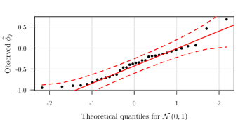
Figure 2: Normal quantile-quantile plot for observations $\widehat{\phi}_{j}$ in Experiment 1.

The normality assumption of the t-test can be easily validated using the normal QQ-plot shown in Figure 2. The plot indicates that no expressive deviations of normality are present, which gives us confidence in using the t test as our inferential procedure of choice, since the sampling distribution of the means will be even closer to a Normal variable than the data distribution, diluting whatever small deviations from normality may be present.

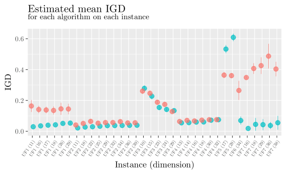
Figure 3: Top: $95\%$ confidence intervals on the means of individual IGD values of each algorithm on each sampled instance. Bottom: Density estimates of IGD for MOEA/D and MOEA/D-DE on each sampled instance. Notice the discrepant performance of MOEA/D-DE on instance UF5.

Finally, it is important to reinforce that these results could also be used to motivate further analyses of the performance of these two algorithms for problems belonging to the problem class of interest, even before proceeding to the full, exhaustive test on all available instance. For example, the individual IGD distributions and mean values of each algorithm on each instance, presented in Figure 3, suggest that both algorithms encounter difficulties when solving UF5 (and, to a lesser extent, UF3) instances, which could motivate a more focused investigation into the reasons for these poor performance profiles, and on possible algorithmic improvements to remedy this problem. A natural follow-up to the experiment presented in this first example would be to broaden the investigation to include the full available test set, in which case the proposed methodology could still be useful in defining the number of repetitions to be performed for each algorithm on each test instance, as well as the expected statistical power of whatever subgroup comparisons the researcher could deem interesting.

5.2 Experiment 2

As mentioned in Section 4.5, the proposed methodology can also be useful in situations when the researcher uses a predefined set of benchmark instances to compare two algorithms. To illustrate this case, we used a set of $200$ large instances of the unrelated parallel machines problem with sequence dependent setup times, provided by Vallada and Ruiz [57] for calibration experiments. Currently the best results for this problem are those presented by Santos et al. [52] using a simulated annealing algorithm with six neighborhood structures (Shift, Switch, Task move, Swap, Two-Shift, and Direct swap), randomly selected at each trial move..

Preliminary tests suggest that the most influential neighborhood structure for this case is Task move, which presents the largest expected improvement value across a wide range of problem sizes. To isolate and quantify the effect of this specific neighborhood structure to the performance of the method, two versions of the algorithm were compared: a full version, which is the original algorithm equipped with all six neighborhood structures; and a no-task-move version, which uses exactly the same structure but does not include the Task move neighborhood. As mentioned above, these two versions were tested on the calibration test set proposed by Vallada and Ruiz [57], which features $200$ large instances with $M\in\left\{10,15,20,25,30\right\}$ machines and $N\in\left\{50,100,150,200,250\right\}$ jobs. All algorithmic aspects were set exactly as in [52], with the stop criteria employed at each instance being the total run time, calculated as a function of instance size following guidelines from the original references [57, 52].

Given that the number of instances is predefined, there is no need to calculate it using the approach presented in Section 4.2. Instead, we used the proposed methodology to estimate the power curve of the experiment, that is, the expected sensitivity of this comparison to detect effects of different magnitudes. This is illustrated in Figure 4, which was derived assuming that the desired significance of the experiment is $\alpha=0.05$, and that a t-test test will be performed using a one-sided alternative hypothesis, since we have a prior expectation that the full version algorithm should be better than the no-task-move, and are interested in testing and quantifying this effect.

Figure 4: Expected sensitivity of experiment 2 to different effect sizes, for a t-test test with a one-sided alternative hypothesis. With $200$ instances we can be fairly confident that the experiment will be able to identify mean performance gains greater than approximately 0.2 standard deviations.

As suggested in the figure, this experiment has a reasonable probability of detecting mean performance gains due to the use of the Task move neighborhood structure greater than about $0.2$ standard deviations. Smaller differences in mean performance, particularly under about $0.1$ standard deviations, can go undetected, but in terms of impact on the expected behavior of the algorithm these would be really minor effects.

The experiment was performed using the proposed method for iteratively estimating the required number of repetitions for each algorithm on each of the $200$ instances. The experimental parameters were set as $se^{*}=0.05$ on the percent differences, $n_{0}=15$ and $n_{max}=150$. The standard errors were calculated using the parametric formulas provided in Section 4.1.2. A t test performed on the resulting data suggested significant differences at the $95\%$ confidence level ($p<2\times 10^{-16},df=199$, against a one-sided, lower $H_{1}$) with an estimated paired mean difference of $\widehat{\mu}_{D}=-0.361$ ($CI_{0.95}=\left[-0.380,-0.342\right]$), which means that the expected impact of the Task move neighborhood on the performance of the algorithm, for an instance belonging to the same problem family defined by the test, set is a reduction of $\left(36.1\pm 1.9\right)\%$ in the makespan of the final solution returned.

Notice that further analyses could (and should) be performed on this same data, to refine the conclusions and, possibly, suggest new lines of inquiry. For instance, while the overall expected improvement due to the use of Task move in the pool of possible movements is quantified as $\left(36.1\pm 1.9\right)\%$, knowledge, e.g., of instance size can improve the estimation accuracy of performance gains. This is illustrated in Figure 5, which suggests that, while the use of Task move provides relevant improvements across all problem sizes tested, its effect increases with the number of machines ($M$) and decreases with the number of jobs ($N$). A detailed quantification of these effects and the reasons behind them is, however, outside the scope of the present work.

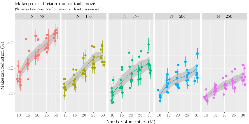
Figure 5: Percent gains in performance attributable to using the Task-move neighborhood. The y-axis indicates how much lower the average makespan was for the full algorithm in comparison to the no-task-move version (notice that the y-axis is vertically reversed). Vertical lines represent the standard errors of each observation. The x-coordinates of the observations were perturbed slightly around their true values ($M=\left\{10,15,20,25,30\right\}$), for visualization purposes.

6 Conclusions

Experimental comparisons play a central role in the research and development of optimization heuristics. In this work we proposed a methodology to address an often neglected aspect of the design of experiments for the comparison of two algorithms on a given problem class, namely the determination of adequate sample sizes, in terms of the amount of problem instances to be employed in a given comparison as well as the number of repeated runs of each algorithm on each instance.

Prior to describing the methodology for sample size calculations, it was important to formally define the algorithm comparison problem considered in our work. This definition, presented in Section 2, was important for two reasons: first, it allowed us to delimit the scope of the scientific and statistical questions of interest in this particular paper, and to formalize the population which our statistical procedures would attempt to interrogate. Second, we hope that it may provide statistical grounds for future discussions and developments in the field of experimental comparisons of algorithms.

Based on the concepts defined in Sections 2 and 3, the proposed methodology for calculating the relevant sample sizes for the comparison of two algorithms on a given problem class was presented in Section 4. The determination of the number of instances is based on considerations of practically relevant differences and on the desired statistical power to detect them. Analytic formulas were presented for the parametric case, using both one-sided and two-sided alternative hypotheses. Nonparametric approximations based on the asymptotic relative efficiency of the Wilcoxon signed-ranks and the binomial sign test were also provided.

The number of runs of each algorithm on each instance is determined iteratively, approximating optimal sample size ratios for the reduction of the uncertainty associated with the estimation of paired differences in performance. Analytic solutions for the optimal ratio of sample sizes were provided for the simple and percent difference cases, based on the assumption of normality of the sampling distribution of the means. These results were also useful as approximations for the calculation of the standard errors using bootstrap, for cases in which the assumption of normality described in Section 4.3 cannot be expected or guaranteed.

Examples of application were provided in Section 5, illustrating the potential of the proposed methodology to provide researchers in the field with a methodologically sound, reproducible way of determining the required numbers of instances and runs, as well as to identify limitations with existing experimental benchmark sets. Two common situations were discussed: the first, in which the researcher needs to determine how many instances of a given problem class to use for a given test, as well as how many runs each algorithm should perform on each instance; and a second one, which focused on the use of the proposed methodology for an experiment dealing with a fixed-size, predefined benchmark set, in which case the assessment of the sensitivity of the experiment to different effect sizes replaces the estimation of the required number of instances to achieve a redefined statistical power.

It is important to reinforce that the proposed methodology is by no means an universal way to test algorithms: when the goal of the experiment is to characterize an heuristic, how robust it is and its best / worst case performance behavior, different methodologies can and should be employed. However, such extensive experimentation is prohibitive in a number of scenarios, such as in several cases of applied engineering optimization [56] or when comparing heuristics on very large, time-consuming instances.

One of the main aims of this work was to lay the statistical and methodological groundwork for the calculation of required sample sizes in the experimental comparison of algorithms. While the developments and results presented do fulfill this particular goal, there are a number of limitations and possibilities of continuity that can be explored. We finish this work by examining a few of the most promising ones.

6.1 Limitations and Possibilities

Possibly the main limitations of the methodology developed in this paper are, in order of severity: (i) the fact that it is only defined for the comparison of two algorithms; (ii) the fact that the definition of the number of instances is performed a priori, using a fixed sample size methodology; and (iii) the fact that only centrality statistics (the mean and, to a certain extent, the median) were considered. Below we offer a brief discussion these three points, and offer our views of what can be done to further extend the proposed methodology.

Regarding the number of algorithms considered in the comparison, a natural next step of this work is to extend the sample size estimation methodologies for multiple algorithms. This can be achieved in a relatively straightforward manner for the estimation of the number of instances, using standard formulas for either omnibus tests (e.g., ANOVA, Friedman) or planning directly for the eventual post-hoc pairwise comparisons [45]. Estimating the number of runs, however, will require greater improvements on the method proposed in this work, probably based on the definition of standard error thresholds for each individual algorithm on each instance, instead of on the standard error of the differences.

While the a priori definition of the number of instances provides a reasonable expectation of statistical power for a given MRES, the required sample size may be considerably smaller if the actual effect size is much larger than the predefined $d^{*}$. Using sequential analysis methodologies, such as the ones commonly employed in clinical trials or industrial settings [12, 3], may result in a reduced number of instances being necessary to determine the existence of differences between two (or eventually more) algorithms, and represent another possibility of continuity for this work. In this aspect, Bayesian alternatives to the comparison of algorithms can be of particular interest, since they may allow the aggregation of existing knowledge in the form of prior probability distributions, as well as the incremental aggregation of observations without the need for cumbersome significance corrections [40].

The possibility of using the methodology defined in this work as a framework for comparisons of algorithms according to different statistics – e.g., variances, rates of convergence, regression coefficients, or best/worst cases – is yet another promising direction. While most experiments still focus on average (mean/median) cases, the need for methodologically sound comparisons of other quantities has long been recognized [34, 25], and we believe the methodology presented in this paper can be easily adapted for such comparisons. First, the bootstrap approach for the calculation of the number of runs can be extended to different measures of paired differences in performance - medians, quantiles, or other statistics - in a relatively straightforward manner (using balanced samples if needed, or deriving optimal ratios for these statistics). Moreover, standard statistical tests for other quantities tend to be readily available, as well as analytic formulas for power and sample size [45], providing a rich basis upon which better, more comprehensive protocols for algorithmic comparisons can be built.

References

- [1] del Amo, I.G., Pelta, D.A., González, J.R., Masegosa, A.D.: An algorithm comparison for dynamic optimization problems. Applied Soft Computing 12(10), 3176–3192 (2012).
- [2] Barr, R.S., Golden, B.L., Kelly, J.P., Resende, M.G.C., Stewart, W.R.: Designing and reporting on computational experiments with heuristic methods. Journal of Heuristics 1(1), 9–32 (1995).
- [3] Bartroff, J., Lai, T., Shih, M.C.: Sequential Experimentation in Clinical Trials: Design and Analysis. Springer (2013)
- [4] Bartz-Beielstein, T.: New Experimentalism Applied to Evolutionary Computation. Ph.D. thesis, Universität Dortmund, Germany (2005)
- [5] Bartz-Beielstein, T.: Experimental Research in Evolutionary Computation. Springer (2006)
- [6] Bartz-Beielstein, T., Chiarandini, M., Paquete, L., Preuss, M.: Experimental Methods for the Analysis of Optimization Algorithms. Springer (2010)
- [7] Bausell, R., Li, Y.F.: Power analysis for experimental research: a practical guide for the biological, medical and social sciences. Cambridge University Press (2006)
- [8] Benavoli, A., Corani, G., Mangili, F., Zaffalon, M., Ruggeri, F.: A bayesian wilcoxon signed-rank test based on the dirichlet process. In: 30th International conference on machine learning, pp. 1026–1034 (2014)
- [9] Birattari, M.: On the estimation of the expected performance of a metaheuristic on a class of instances: how many instances, how many runs? Tech. Rep. IRIDIA/2004-001, Université Libre de Bruxelles, Belgium (2004)
- [10] Birattari, M.: Tuning Metaheuristics – A Machine Learning Perspective. Springer Berlin Heidelberg (2009)
- [11] Birattari, M., Dorigo, M.: How to assess and report the performance of a stochastic algorithm on a benchmark problem: Mean or best result on a number of runs? Optimization Letters 1, 309–311 (2007)
- [12] Botella, J., Ximénez, C., Revuelta, J., Suero, M.: Optimization of sample size in controlled experiments: The CLAST rule. Behavior Research Methods 38(1), 65–76 (2006).
- [13] Bradley Efron, R.T.: An Introduction to the Bootstrap, 1 edn. Chapman and Hall (1994)
- [14] Campelo, F., Batista, L.S., Aranha, C.: The MOEADr package – a component-based framework for multiobjective evolutionary algorithms based on decomposition. Submitted: Journal of Statistical Software (2017)
- [15] Campelo, F., Takahashi, F.: CAISEr: Comparison of Algorithms with Iterative Sample Size Estimation (2017). URL https://CRAN.R-project.org/package=CAISEr
- [16] Carrano, E.G., Wanner, E.F., Takahashi, R.H.C.: A multicriteria statistical based comparison methodology for evaluating evolutionary algorithms. IEEE Transactions on Evolutionary Computation 15(6), 848–870 (2011).
- [17] Chow, S.C., Wang, H., Shao, J.: Sample Size Calculations in Clinical Research. CRC Press (2003)
- [18] Coffin, M., Saltzman, M.J.: Statistical analysis of computational tests of algorithms and heuristics. INFORMS Journal on Computing 12(1), 24–44 (2000).
- [19] Crawley, M.: The R Book, 2nd. edn. Wiley (2013)
- [20] Czarn, A., MacNish, C., Vijayan, K., Turlach, B.: Statistical exploratory analysis of genetic algorithms: the importance of interaction. In: Proceedings of the 2004 IEEE Congress on Evolutionary Computation. Institute of Electrical & Electronics Engineers (IEEE) (2004).
- [21] Davison, A.C., Hinkley, D.V.: Bootstrap methods and their application. Cambridge University Press (1997)
- [22] Demšar, J.: Statistical comparisons of classifiers over multiple data sets. Journal of Machine Learning Research 7, 1–30 (2006)
- [23] Derrac, J., García, S., Hui, S., Suganthan, P.N., Herrera, F.: Analyzing convergence performance of evolutionary algorithms: A statistical approach. Information Sciences 289, 41–58 (2014)
- [24] Derrac, J., García, S., Molina, D., Herrera, F.: A practical tutorial on the use of nonparametric statistical tests as a methodology for comparing evolutionary and swarm intelligence algorithms. Swarm and Evolutionary Computation 1(1), 3–18 (2011).
- [25] Eiben, A., Jelasity, M.: A critical note on experimental research methodology in EC. In: Proceedings of the 2002 IEEECongress on Evolutionary Computation. Institute of Electrical & Electronics Engineers (IEEE) (2002).
- [26] Fieller, E.C.: Some problems in interval estimation. Journal of the Royal Statistical Society. Series B (Methodological) 16(2), 175–185 (1954)
- [27] Franz, V.: Ratios: A short guide to confidence limits and proper use (2007). URL https://arxiv.org/pdf/0710.2024v1.pdf
- [28] García, S., Fernández, A., Luengo, J., Herrera, F.: A study of statistical techniques and performance measures for genetics-based machine learning: accuracy and interpretability. Soft Computing 13(10), 959–977 (2009).
- [29] García, S., Fernández, A., Luengo, J., Herrera, F.: Advanced nonparametric tests for multiple comparisons in the design of experiments in computational intelligence and data mining: Experimental analysis of power. Information Sciences 180(10), 2044–2064 (2010).
- [30] García, S., Molina, D., Lozano, M., Herrera, F.: A study on the use of non-parametric tests for analyzing the evolutionary algorithms’ behaviour: a case study on the CEC’2005 Special session on real parameter optimization. Journal of Heuristics 15(6), 617–644 (2008).
- [31] Grissom, R.J., Kim, J.J.: Effect Sizes for Research, 2nd edn. Routledge (2012)
- [32] Hansen, N., Auger, A., Mersmann, O., Tusar, T., Brockhoff, D.: COCO: A platform for comparing continuous optimizers in a black-box setting. CoRR abs/1603.08785 (2016). URL http://arxiv.org/abs/1603.08785
- [33] Hansen, N., Tǔsar, T., Mersmann, O., Auger, A., Brockoff, D.: COCO: The experimental procedure (2016). URL https://arxiv.org/abs/1603.08776
- [34] Hooker, J.N.: Testing heuristics: We have it all wrong. Journal of Heuristics 1(1), 33–42 (1996)
- [35] Hurlbert, S.H.: Pseudoreplication and the design of ecological field experiments. Ecological Monographs 54(2), 187–211 (1984).
- [36] Jain, R.K.: The Art of Computer Systems Performance Analysis. John Wiley and Sons Ltd (1991)
- [37] Johnson, D.: A theoretician’s guide to the experimental analysis of algorithms. In: M. Goldwasser, D. Johnson, C. McGeoch (eds.) Data Structures, Near Neighbor Searches, and Methodology: Fifth and Sixth DIMACS Implementation Challenges, DIMACS Series in Discrete Mathematics and Theoretical Computer Science, vol. 59, pp. 215–250. American Mathematical Society (2002)
- [38] Jones, D.R., Schonlau, M., Welch, W.J.: Efficient global optimization of expensive black-box functions. Journal of Global Optimization 13(4), 455–492 (1998)
- [39] Krohling, R.A., Lourenzutti, R., Campos, M.: Ranking and comparing evolutionary algorithms with hellinger-TOPSIS. Applied Soft Computing 37, 217–226 (2015).
- [40] Kruschke, J.K.: Doing Bayesian Data Analysis: A Tutorial with R and BUGS, 1st edn. Academic Press, Inc. (2010)
- [41] Lazic, S.E.: The problem of pseudoreplication in neuroscientific studies: is it affecting your analysis? BMC Neuroscience 11(5), 397–407 (2010).
- [42] Lenth, R.V.: Some practical guidelines for effective sample size determination. The American Statistician 55(3), 187–193 (2001)
- [43] Li, H., Zhang, Q.: Multiobjective optimization problems with complicated pareto sets, MOEA/d and NSGA-II. IEEE Transactions on Evolutionary Computation 13(2), 284–302 (2009).
- [44] Maravilha, A.L., Pereira, L.M., Campelo, F.: Statistical characterization of neighborhood structures for the unrelated parallel machine problem with sequence-dependent setup times. In preparation
- [45] Mathews, P.: Sample Size Calculations: Practical Methods for Engineers and Scientists, 1st edn. Matthews Malnar & Bailey Inc. (2010)
- [46] McGeoch, C.C.: Feature article—toward an experimental method for algorithm simulation. INFORMS Journal on Computing 8(1), 1–15 (1996).
- [47] Montgomery, D.C., Runger, G.C.: Applied Statistics and Probability for Engineers, 6th edn. Wiley (2013)
- [48] Mori, T., Sato, Y., Adriano, R., Igarashi, H.: Optimal design of RF energy harvesting device using genetic algorithm. Sensing and Imaging 16(1) (2015)
- [49] Nuzzo, R.: Scientific method: Statistical errors. Nature 506(7487), 150–152 (2014)
- [50] R Core Team: R: A Language and Environment for Statistical Computing. R Foundation for Statistical Computing, Vienna, Austria (2017). URL https://www.R-project.org/
- [51] Ridge, E.: Design of Experiments for the Tuning of Optimisation Algorithms. Ph.D. thesis, The University of York, UK (2007)
- [52] Santos, H.G., Toffolo, T.A., Silva, C.L., Berghe, G.V.: Analysis of stochastic local search methods for the unrelated parallel machine scheduling problem. International Transactions in Operational Research 00 (2016). URL https://doi.org/10.1111/itor.12316
- [53] Sawilowsky, S.S.: New effect size rules of thumb. Journal of Modern Applied Statistical Methods 8(2), 597–599 (2009)
- [54] Shaffer, J.P.: Multiple hypothesis testing. Annual review of psychology 46(1), 561–584 (1995)
- [55] Sheskin, D.J.: Handbook of Parametric and Nonparametric Statistical Procedures. Taylor & Francis (2011)
- [56] Tenne, Y., Goh, C.K.: Computational Intelligence in Expensive Optimization Problems. Springer (2010)
- [57] Vallada, E., Ruiz, R.: A genetic algorithm for the unrelated parallel machine scheduling problem with sequence dependent setup times. European Journal of Operational Research 211(3), 612–622 (2011)
- [58] Yuan, B., Gallagher, M.: Statistical racing techniques for improved empirical evaluation of evolutionary algorithms. Parallel Problem Solving From Nature - PPSN VIII 3242, 172–181 (2004)
- [59] Yuan, B., Gallagher, M.: An improved small-sample statistical test for comparing the success rates of evolutionary algorithms. In: Proceedings of the 11th Annual conference on Genetic and evolutionary computation - GECCO09. Association for Computing Machinery (ACM) (2009).
- [60] Zhang, Q., Li, H.: MOEA/d: A multiobjective evolutionary algorithm based on decomposition. IEEE Transactions on Evolutionary Computation 11(6), 712–731 (2007).
- [61] Zhang, Q., Zhou, A., Zhao, S., Suganthan, P., Liu, W., Tiwari, S.: Multiobjective optimization test instances for the cec 2009 special session and competition. Tech. Rep. CES-887, University of Essex (2008). URL http://dces.essex.ac.uk/staff/zhang/moeacompetition09.htm. (revised on 20/04/2009)
- [62] Zitzler, E., Thiele, L., Laumanns, M., Fonseca, C., Fonseca, V.: Performance assessment of multiobjective optimizers: An analysis and review. IEEE Transactions on Evolutionary Computation 7(2), 117–132 (2003)