Estimation of spectrum and parameters of relic gravitational waves using space-borne interferometers

Abstract

We present a study of spectrum estimation of relic gravitational waves (RGWs) as a Gaussian stochastic background from output signals of future space-borne interferometers, like LISA and ASTROD. As the target of detection, the analytical spectrum of RGWs generated during inflation is described by three parameters: the tensor-scalar ratio, the spectral index and the running index. The Michelson interferometer is shown to have a better sensitivity than Sagnac, and symmetrized Sagnac. For RGW detection, we analyze the auto-correlated signals for a single interferometer, and the cross-correlated, integrated as well as un-integrated signals for a pair of interferometers, and give the signal-to-noise ratio (SNR) for RGW, and obtain lower limits of the RGW parameters that can be detected. By suppressing noise level, a pair has a sensitivity 2 orders better than a single for one year observation. SNR of LISA will be 4-5 orders higher than that of Advanced LIGO for the default RGW. To estimate the spectrum, we adopt the maximum likelihood (ML) estimation, calculate the mean and covariance of signals, obtain the Gaussian probability density function (PDF) and the likelihood function, and derive expressions for the Fisher matrix and the equation of the ML estimate for the spectrum. The Newton-Raphson method is used to solve the equation by iteration. When the noise is dominantly large, a single LISA is not effective for estimating the RGW spectrum as the actual noise in signals is not known accurately. For cross-correlating a pair, the spectrum can not be estimated from the integrated output signals either, and only one parameter can be estimated with the other two being either fixed or marginalized. We use the ensemble averaging method to estimate the RGW spectrum from the un-integrated output signals. We also adopt a correlation of un-integrated signals to estimate the spectrum and three parameters of RGW in a Bayesian approach. For all three methods, we provide simulations to illustrate their feasibility.

Key Words: gravitational waves, cosmological parameters, instrumentation: detectors, early universe.

1 Introduction

Gravitational waves (GWs) are a prediction of Einstein’s theory of general relativity, and have been the subject of theoretical study and continuous detection hunting. There are two kinds of GW, i.e, the first includes those generated by astrophysical processes such as inspiral of compact binaries, merging of massive black holes, super-massive black hole binaries [1], etc. The frequencies of these sources are typically in the range $f\sim 10^{-9}-10^{3}$ Hz. Examples are GW150914, GW151226 and GW170104 from merging of binary black holes and GW170817 from the binary neutron star inspiral that was recently reported by Advanced LIGO and Advanced Virgo as the first direct detections [2, 3, 4].

Another kind is the relic gravitational wave (RGW), which is generated during the inflation stage of cosmic expansion, as generically predicted by inflation models [6]. RGW carries crucial information about the very early Universe, such as the energy scale and slope of inflation potential, the initial quantum states during inflation [7, 8], as well as the reheating process [9]. This is because, to the linear level of metric perturbations, RGW is independent of other matter components and its propagation is almost free. The influences due to neutrinos free-streaming [10, 11], quark-hadron transition and $e^{+}e^{-}$ annihilation are minor modifications [12]. This is in contrast to the scalar metric perturbation, which is always coupled to cosmic matters and whose short wavelength modes have gone into nonlinear evolution at present. The second-order perturbation beyond the linear perturbation has been also studied for RGW [13, 14].

RGW has several interesting properties that are quite valuable for GW detection. It is a stochastic background of spacetime fluctuations distributed everywhere in the present Universe, just like the cosmic microwave background (CMB). Moreover, RGW also exists all the time, and its spectrum changes very slowly on a cosmic time-scale, so that its detections can be repeated at any time, in contrast to short-duration GW radiations events such as merging of binaries. Another big plus of RGW for detections is that its frequency range is extremely broad, stretching over $f\sim 10^{-18}-10^{11}$ Hz. Thus, RGW is a major target for various kinds of GW detectors at various frequency bands, using various technologies [15], such as CMB anisotropies and polarization measurements ($10^{-18}-10^{-16}$ Hz), by COBE [16], WMAP [17, 18], Planck [19, 20], etc, pulsar timing arrays ($10^{-9}-10^{-7}$ Hz) [21], space laser interferometer ($10^{-5}-10^{0}$ Hz), for LISA [22, 25, 26], ($10^{-6}-10^{0}$ Hz) for ASTROD [27] and for Tianqin and Taiji [28], ground-based laser interferometers $(10-2000$ Hz), like LIGO [29, 30, 31], Virgo [32], GEO [33], KAGRA [34] etc, cavity detectors ($\sim 4000$ Hz) [35], waveguide detectors ($\sim 10^{8}$ Hz) [36] and polarized laser beam detectors ($\sim 10^{10}$ Hz) [37].

A primary feature of the RGW spectrum is that it has higher amplitude at lower frequencies [7]. The highest amplitude is located around ($10^{-18}-10^{-16}$)Hz which is the target of CMB measurements. So far, the magnetic polarization $C^{BB}_{l}$ induced by RGW [38] has not yet been detected, and only some constraint is given in terms of the tensor-scalar ratio of metric perturbations $r<0.1$ [19, 20]. On the other hand, Advanced LIGO-Virgo so far has not detected RGW, but rather has only been applied to predict a total stochastic GW background with amplitude $1.8^{+2.7}_{-1.3}\times 10^{-9}$ near 25 Hz contributed together by unresolved binaries, RGW, etc [5]. In between is the band of the space-borne facilities, LISA and ASTROD, where the amplitude of RGW is higher by 5-6 orders than that in the LIGO band. This great enhancement increases the chance for space-borne interferometers to detect RGWs if their sensitivity level is comparable to LIGO.

In this paper, we shall study RGW detection by space-borne interferometers, such as LISA and ASTROD and the like, and show how to estimate the spectrum and parameters of RGW from output signals of future observations. For this purpose, we shall first briefly introduce the theoretical RGW spectrum as a scientific target, resulting from an analytical solution that covers from inflation to the present acceleration [7]. Accurate estimation of this spectrum will also confirm the details of inflation for the very early Universe. In this sense, this will be a direct detection of inflation. For the RGW spectrum in this paper, we focus on three parameters determined by inflation: the tensor-scalar ratio $r$, the spectral index $\beta$ and the spectral running index $\alpha_{t}$ [15, 8]. Small modifications of RGW in Refs.[10, 11, 12] are not considered. We do not consider the Doppler modulation due to orbital motion, or related causes [39]. One of the main obstacles to detecting RGW is the stochastic foreground of a GW resulting from the superposition of a large number of unresolved astrophysical sources. To have a definite model of the power spectrum of the stochastic foreground, one has to know the spectrum for each type of source, as well as the evolution of each type. There are several categories of these source types. Due to the large abundance, Galactic white dwarf binaries are generally considered one of the main components of the foreground in the $\sim 10^{-3}$ Hz frequency band [40]. Refs. [41, 42, 43, 44] provide several models of the foreground generated by distribution of these binaries. Ref. [45] have studied a stochastic foreground from massive black hole binaries and its contribution to the LISA datastream. Ref. [46] show the possibility of a foreground generated by an AM CVn binary system. To explore the effects of these foreground models on a spaced-based detector, simulation methods to generate a foreground data stream for LISA have been studied by the Mock LISA data challenge project [47] and other groups [48, 49]. Based on these dummy datastreams, several techniques for model selection and parameter estimation have been developed [42, 51, 50, 49, 44]. Refs. [52, 51] have provided methods to detect resolvable sources in a foreground of unresolvable sources. Ref. [44] investigated approaches to discriminate the GW background from a stochastic foreground according to the differences in spectral shapes and time modulation of the signal. Currently, the foreground is still under intensive study but is not fully understood. At this stage of our study we do not include the foreground in this paper.

GW radiation from a finite source usually has a definite waveform (fixed direction, amplitude, etc) and the match-filter method [53] is commonly used to estimate the waveform against certain theoretical templates. Refs.[55, 54] studied the methods of parameter estimation for ground-based LIGO detectors. Refs.[56, 57] studied detection of a GW radiated from merging compact binaries using LISA detectors. In contrast, RGW is of stochastic nature, incident from all directions, containing modes of all possible frequencies and amplitudes. Refs.[58, 59] systematically studied detection of RGW using LIGO, obtained a formula for signal-to-noise ratio (SNR) as a criterion for detection. Ref.[60] discussed the possible detection by eLISA of GW backgrounds due to first-order phase transitions, cosmic strings, bubble collision, etc. Ref.[61] discussed possibility of RGW detection by LISA. So far in literature, however, RGW detection by space-based interferometers has not been systematically studied, in particular, estimation for the RGW spectrum has not been analyzed. We shall derive formulations of estimation of the RGW spectrum, using a single or a pair of space-based interferometers like LISA and ASTROD etc.

For this purpose, we shall briefly examine the three kinds of interferometers: Michelson, Sagnac and symmetrized Sagnac [62, 65, 63, 26, 66, 67, 64, 68, 70, 69, 71], whose sensitivity depends on both the noise and transfer function, which in turn depends on the detector geometry. We shall show explicitly that the Michelson has the best sensitivity, which will be taken as a default interferometer. For a single interferometer in space, we give SNR and a criterion to detect RGW. As a Gaussian stochastic background, RGW is similar to CMB anisotropies, and the statistical methods employed in CMB studies can be used [72, 73, 18]. We shall apply the maximum likelihood (ML) method [74] to estimate the RGW spectrum. We give the probability density function (PDF) explicitly, and derive the estimation equation of an RGW spectrum. However, in practice, our knowledge of the spectrum of noise that is actually occurring in the detector is not sufficient so that a single case is not effective to estimate the RGW spectrum when the noise is dominantly large.

For a pair, the noise level will be suppressed by cross-correlation. We shall introduce cross-correlated, integrated output of the pair, in a fashion similar to the ground-based LIGO [59], calculate the overlapping reduction function, give the sensitivity and compare with that of a single case, and analyze possible detection and constraints on RGW parameters. However, the spectrum as a function of frequency can not be estimated from the integrated output, since the frequency-dependence has been lost in integration. One can estimate only one parameter in the Bayesian approach by ML-estimation, using the Newton-Raphson method [73, 18, 75]. To estimate the spectrum, we propose the ensemble averaging method, and directly take the cross-product of un-integrated output signals from a pair. The method does not depend on precise knowledge of the noise spectrum. We estimate the spectrum using simulated data for illustration, but one can not estimate the parameters. Ref. [76] suggested a method of correlation for un-integrated signals, by which the whole frequency range of the data is to be divided into many small segments of frequency, and the mean value of a correlation variable over each small segment is taken as the representative point for the segment. In this way, as an approximation, the correlation variable as a function of frequency is defined on the whole range. Ref. [76] considered a simple power-law spectrum of stochastic GW, analyzing the resolution of parameter estimation, but did not give an estimation of the spectrum. We adopt this as the third method to estimate the RGW spectrum by ML-estimation, as well as the three parameters ($r$, $\beta$, $\alpha_{t}$) simultaneously in a Bayesian approach. For all these three methods for a pair, we shall provide numerical simulations, demonstrating their feasibility.

The outline of the paper is as follows. In Section 2, we give a short review of the theoretical RGW spectrum. In Section 3 we compare briefly the sensitivity of three types of interferometers, and give a constraint on RGW by a single Michelson in space. In Section 4, we examine signals from a single by the ML method and show that it is not effective to estimate the RGW spectrum when the noise is dominantly large. Section 5 is about the cross-correlated, integrated output signals for a pair. In Section 6, we show that the integrated output signals from a pair can be used to estimate one parameter, but not the spectrum. In Section 7 we use the ensemble average method to estimate the spectrum directly. In Section 8, we use the correlation method for un-integrated output signals to estimate the spectrum and parameters of RGW. Appendix A gives the derivation of the Fisher matrix for a pair.

2 Relic Gravitational Wave

This section reviews the main properties of RGWs relevant to detection by LISA. RGW as the tensor metric perturbations of spacetime is generated during inflation and exists as a stochastic background of fluctuations in the Universe. It has an extremely broad spectrum, ranging from $10^{-18}$ Hz to $10^{11}$ Hz. In particular, it has a characteristic amplitude of $10^{-22}\sim 10^{-24}$ around $f\sim 10^{-3}$ Hz (see Fig.1) and can serve as a target for LISA. The exact solution and corresponding analytical spectrum of RGW have been obtained [7, 8] that cover the whole course of expansion, from inflation, reheating, radiation, matter, to the present accelerating stage.

For a spatially flat Robertson-Walker spacetime, the metric with tensor perturbation is

$$ds^{2}=a(\tau)^{2}[-d\tau^{2}+(\delta_{ij}+h_{ij})dx^{i}dx^{j}]$$ (1)

where $h_{ij}$ is the tensor perturbation and $\tau$ is the conformal time. From the inflation to the accelerating expansion, there are five stages, with each stage being described by a power-law scale factor $a(\tau)\propto\tau^{d}$ where $d$ is a constant [7]. The particularly interesting stage is inflation with

$$a(\tau)=l_{0}|\tau|^{1+\beta},\hskip 28.45274pt-\infty<\tau\leq\tau_{1},$$ (2)

where $\beta$ is the spectral index. For the exact de Sitter, $\beta=-2$, and for generic inflation models and $\beta$ can deviate slightly from -2 [7]. The present accelerating stage has

$$a(\tau)=l_{H}|\tau-\tau_{a}|^{-\gamma},\hskip 28.45274pt\tau_{E}\leq\tau\leq\tau_{H},$$ (3)

where $\gamma=2.018$ is taken for $\Omega_{\Lambda}=0.71$ [8]. The normalization is taken as $a(\tau_{H})=l_{H}=\gamma/H_{0}$, where $H_{0}$ is the present Hubble constant.

The tensorial perturbation $h_{ij}$ as a quantum field is decomposed into the Fourier modes,

$$h_{ij}({\bf x},\tau)=\int\frac{d^{3}k}{(2\pi)^{3/2}}\sum_{A={+,\times}}\epsilon^{A}_{ij}({\bf k})\left[a^{A}_{\bf k}h^{A}_{k}(\tau)e^{i\bf{k}\cdot\bf{x}}+a^{A\,\dagger}_{\bf k}h^{A\,*}_{k}(\tau)e^{-i\bf{k}\cdot\bf{x}}\right],\,\,\,\,{\bf k}=k\hat{k},$$ (4)

where $a^{A}_{\bf k}$ and $a^{A\,\dagger}_{\bf k}$ are the annihilation and creation operators respectively of a graviton with wavevector $\bf k$ and polarization $A$, satisfying the canonical commutation relation

$$\left[a^{A}_{\bf k},\,a^{A^{\prime}\,\dagger}_{\bf k^{\prime}}\right]=\delta_{AA^{\prime}}\,\delta^{3}({\bf k-k^{\prime}}).$$ (5)

Two polarization tensors satisfy

$$\epsilon^{A}_{ij}({\bf k})\delta_{ij}=0,\,\,\,\,\epsilon^{A}_{ij}({\bf k})k^{i}=0,\,\,\,\,\epsilon^{A}_{ij}({\bf k})\epsilon^{A^{\prime}}_{ij}({\bf k})=2\delta_{AA^{\prime}},$$ (6)

and can be taken as

$$\epsilon_{ij}^{+}({\bf k})=(l_{i}l_{j}-m_{i}m_{j}),\,\,\,\,\epsilon_{ij}^{\times}({\bf k})=(l_{i}m_{j}+m_{i}l_{j}),$$

where $\bf l$, $\bf m$ are mutually orthogonal unit vectors normal to $\bf k$. In fact, as an observed quantity for LISA, RGW can be also treated as a classical, stochastic field

$$h_{ij}(\tau,x)=\int\frac{d^{3}k}{(2\pi)^{3/2}}\sum_{A=\times,+}\epsilon^{A}_{ij}({\bf k})h^{A}_{k}(\tau)e^{i\mathbf{k\cdot x}},$$ (7)

where the $k$-mode $h^{A}_{k}$ is stochastic, independent of other modes. The physical frequency at present is related to the conformal wavenumber via $f=ck/2\pi a(\tau_{H})$ [7]. For RGW, the two polarization modes $h^{+}_{k}$ and $h^{\times}_{k}$ are assumed to be independent and statistically equivalent, so that the superscript $+,\times$ can be dropped, and the wave equation is

$$h^{\prime\prime}_{k}(\tau)+2\frac{a^{\prime}(\tau)}{a(\tau)}h^{\prime}_{k}(\tau)+k^{2}h_{k}(\tau)=0.$$ (8)

The quantum state during inflation is taken to be $|0\rangle$ such that

$$a^{s}_{\bf k}|0\rangle=0,\,\,$$ (9)

i.e, only the vacuum fluctuations of RGW are present during inflation, and the solution of RGW is

$$h_{k}(\tau)=\frac{\sqrt{32\pi G}}{a(\tau)}\sqrt{\frac{\pi k|\tau|}{2k}}\left(-ie^{-i\pi\beta/2}\right)H^{(2)}_{\beta+\frac{1}{2}}(k|\tau|),\,\,\,\,-\infty<\tau\leq\tau_{1}\,$$ (10)

which is the positive-frequency mode $h_{k}\rightarrow\frac{\sqrt{32\pi G}}{a(\tau)}\frac{1}{\sqrt{k}}e^{-ik\tau}$ and gives a zero point energy $\frac{1}{2}\hbar\omega$ in each $\bf k$-mode and each polarization in the high frequency limit. The wave equation (8) has been solved also for other subsequent stages, i.e, reheating, radiation dominant, matter dominant and accelerating. The solution of Eq. (8) is simply a combination of two Hankel functions, $\tau^{d-1/2}H^{(1)}_{d-1/2}$ and $\tau^{d-1/2}H^{(2)}_{-d+1/2}$. By continuously joining these stages, the full analytical solution $h_{k}(\tau)$ has been obtained, which covers the whole course of evolution, in particular, for the present stage of acceleration, it is given by [8]

$$h_{k}(\tau)=\frac{\sqrt{32\pi G}}{a(\tau)}\sqrt{\frac{\pi s}{2k}}\bigg{[}e^{-i\pi\gamma/2}\beta_{k}H^{(1)}_{-\gamma-\frac{1}{2}}(s)+e^{i\pi\gamma/2}\alpha_{k}H^{(2)}_{-\gamma-\frac{1}{2}}(s)\bigg{]},\,\,\,\,\,\,\tau_{E}<\tau\leq\tau_{H},$$ (11)

where $s\equiv k(\tau-\tau_{a})$ and the coefficients $\beta_{k},\alpha_{k}$ are Bogoliubov coefficients [77] satisfying $|\alpha_{k}|^{2}-|\beta_{k}|^{2}=1$, and $|\beta_{k}|^{2}$ is the number of gravitons at the present stage, and the expressions $\beta_{k},\alpha_{k}$ are explicitly given by Ref.[8]. The frequency range of space-borne interferometers is much higher than the Hubble frequency $H_{0}\simeq 2\times 10^{-18}$ Hz, so that (11) for these modes becomes

$$h_{k}(\tau)\simeq\frac{\sqrt{32\pi G}}{a(\tau)}\frac{1}{\sqrt{k}}e^{-ik\tau}~{}~{}for~{}~{}k~{}~{}\gg 1/|\tau|.$$ (12)

Hence, for space-borne interferometers, RGW is practically a superposition of stochastic plane waves.

The auto-correlation function of RGW is defined by the following expected value

$$\langle 0|h^{ij}(\textbf{x},\tau)h_{ij}(\textbf{x},\tau)|0\rangle=\frac{1}{(2\pi)^{3}}\int d^{3}k\,|h_{k}|^{2},$$ (13)

where (6) (5) have been used. Defining the power spectrum by

$$\langle 0|h^{ij}(\textbf{x},\tau)h_{ij}(\textbf{x},\tau)|0\rangle\equiv\int_{0}^{\infty}\Delta^{2}_{t}(k,\tau)\frac{dk}{k}\,,$$ (14)

one reads off the power spectrum

$$\Delta^{2}_{t}(k,\tau)=\frac{k^{3}}{2\pi^{2}}|h_{k}(\tau)|^{2},$$ (15)

which is dimensionless. We also use a notation $h(f,\tau_{H})\equiv\sqrt{\Delta^{2}_{t}(k,\tau_{H})}$. In the literature on GW detection, the characteristic amplitude

$$h_{c}(f)\equiv\frac{h(k,\tau_{H})}{2\sqrt{f}}$$ (16)

is often used [78, 79], which has dimension Hz^-1/2. The definition (15) holds for any time $\tau$, from inflation to the accelerating stage.

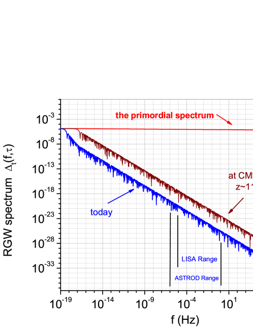
Figure 1: The evolution of RGW spectrum from inflation to the present.

Fig. 1 shows the evolution of the RGW spectrum from inflation to the present acceleration stage. Equivalently, one can also use the spectral energy density $\Omega_{g}\equiv\rho_{g}/\rho_{c}$, where

$$\rho_{g}=\frac{1}{32\pi Ga^{2}}\langle 0|h^{\prime}_{ij}\,h^{\prime ij}|0\rangle$$

is the energy density of RGW [80, 8] and $\rho_{c}=3H_{0}^{2}/8\pi G$ is the critical density. The spectral energy density $\Omega_{g}(f)$ is defined by $\Omega_{g}\equiv\int\Omega_{g}(f)df/f$, and given by

$$\Omega_{g}(f)=\frac{\pi^{2}}{3}h^{2}(f,\tau_{H})\left(\frac{f}{H_{0}}\right)^{2},$$ (17)

which holds for all wavelengths shorter than the horizon.

From the spectrum (15) during inflation, the analytic expressions of spectral, and running spectral indices have been obtained [8] $n_{t}\equiv\frac{d\ln\Delta_{t}^{2}}{d\ln k}\simeq 2\beta+4-\frac{2}{2\beta+3}x^{2}$, $\alpha_{t}\equiv\frac{d^{2}\ln\Delta^{2}_{t}}{d(\ln k)^{2}}\simeq-\frac{4}{2\beta+3}x^{2}$ at $x\equiv|k\tau|\ll 1$, i.e, at far outside horizon, both related to the spectral index $\beta$. In the limit $k\rightarrow 0$, one has the default values

$$n_{t}=2\beta+4\,,\,\,\,\,\alpha_{t}=0,$$ (18)

which hold for the inflation models with $a(\tau)\propto|\tau|^{1+\beta}$. It is incorrect to use $n_{t}$ and $\alpha_{t}$ evaluated at the horizon-crossing $|k\tau|=1$ [81]. With these definitions, the primordial spectrum in the limit $k\rightarrow 0$ is written as

$$\Delta_{t}(k)=\Delta_{R}\,r^{1/2}(\frac{k}{k_{0}})^{\frac{1}{2}n_{t}+\frac{1}{4}\alpha_{t}\ln(\frac{k}{k_{0}})},$$ (19)

where $k_{0}$ is a pivot conformal wavenumber corresponding to a physical wavenumber $k_{0}/a(\tau_{H})=0.002$Mpc^-1, $\Delta_{R}$ is the value of curvature perturbation determined by observations $\Delta_{R}^{2}=(2.464\pm 0.072)\times 10^{-9}$, and $r\equiv\Delta^{2}_{t}(k_{0})/\Delta^{2}_{R}(k_{0})$ is the tensor-scalar ratio, and with $r<0.1$ by CMB observations [20]. The primordial spectrum (19) describes the upper curve (red) during inflation in Fig. 1. The present spectrum $\Delta_{t}(f,\tau_{H})$ and the primordial spectrum $\Delta_{t}(k)$ are overlapped at very low frequencies $f<10^{-18}$ Hz, with both being $\propto r^{1/2}$ as in (19). At $f>10^{11}$ Hz, $\Delta_{t}(f,\tau_{H})$ rises up and has a UV divergence, due to vacuum fluctuations. In Ref.[8], the UV divergence has been adiabatically regularized. Higher values of ($r$, $n_{t}$, $\alpha_{t}$) give rise to higher amplitude of RGW. In particular, a slight increase in $\alpha_{t}$ will enhance greatly the amplitude of RGW in the relevant band. In this paper, we take ($r$, $n_{t}$, $\alpha_{t}$) as the major parameters of RGW.

3 Sensitivity of one interferometer and RGW Detection

We briefly review detection of RGW by a single interferometer, which has been studied before and will be used in this paper later. Figure 2 shows three identical spacecrafts that are placed in space, forming an equilateral triangle. The three arms are of equal length, taken to be $L=5\times 10^{9}$ m by the original design of LISA. when no GW is passing by [22]. This value is taken as an example in our paper. In recent years, the designed arm-length has been modified to be $L=1\times 10^{9}$ m [23] or $L=2.5\times 10^{9}$ m [24]. The recently-proposed projects, like Tianqin and Taiji, also will have $L$ around this value. ASTROD has a longer value of $L=260\times 10^{9}$ m [27]. Spacecraft 1 can shoot laser beams, which are phase-locked, regenerated with the same phase at the spacecrafts 2 and 3, and then sent back [24, 22]. This forms one interferometer. In the presence of a GW, the arm lengths and phases of the beams will fluctuate. Combining the optical paths will produce different interferometers [82]. Here we only discuss three combinations, the Michelson, the Sagnac and the symmetrized Sagnac [70, 69]. To focus on the main issue of spectral estimation for RGW, we do not consider the spacecraft orbital effects, Shapiro delay, etc, caused by the Newtonian potential of the solar system [83, 65, 84].

Figure 2: The three spacecrafts are located at points 1, 2 and 3, and the vectors a,b and c label the direction of the three arms.

3.1 The response tensors for three kinds of interferometers

First, the Michelson interferometer [70, 69, 56, 78] is considered. The optical path difference is proportional to the strain

$$h_{o}=\frac{1}{2L}\left[l_{12}+l_{21}-l_{13}-l_{31}\right],$$ (20)

where $l_{12}$ is the optical path of a photon emitted by spacecraft 1 traveling along arm 1-2, which has arrived at 2, $l_{21}$ is the one reflected at 2 and back to 1, etc. This is the dimensionless strain measured by the interferometer, also called the output response.

Next, the Sagnac interferometer [63] is described. One optical path is 1-2-3-1, and the other is along 1-3-2-1. The strain is proportional to their difference

$$h_{os1}=\frac{1}{3L}\left[l_{13}+l_{32}+l_{21}-l_{12}-l_{23}-l_{31}\right],$$ (21)

where the subscript “1” in $h_{os1}$ refers to vertex 1. In a similar fashion, one can get the output responses at vertex 2 and vertex 3. Last, the symmetrized Sagnac interferometer is examined. Its output response is defined as the average for three Sagnac signals of three vertices, 1, 2 and 3, respectively [85, 71]

$$h_{oss}=\frac{1}{3}(h_{os1}+h_{os2}+h_{os3}).$$ (22)

We shall study the ability to detect RGW with these three kinds of interferometers when implemented in space.

Now we consider the responses of the three kinds of interferometers to a GW. Let a plane GW, with frequency $f$ from a direction $\hat{\Omega}$, pass through the detector located at $\bf r$ and at time $t$. The GW is denoted by $\textbf{h}(\hat{\Omega},f,t,{\bf r})$ as a tensor. The output response of an interferometer is a product

$$h_{o}(\hat{\Omega},f,t,{\bf r})=\textbf{D}(\hat{\Omega},f):\textbf{h}(\hat{\Omega},f,t,{\bf r}).$$ (23)

where $\mathbf{D}(\hat{\Omega},f)$ is the response tensor, depending on the orientation and geometry of LISA and the operating frequency $f$. For the Michelson, the response tensor is [69, 70],

$$\mathbf{D}_{m}(\hat{\Omega},f)=\frac{1}{2}((\textbf{a}\otimes\textbf{a})\mathcal{T}_{m}(\textbf{a}\cdot\hat{\Omega},f)-(\textbf{c}\otimes\textbf{c})\mathcal{T}_{m}(-\textbf{c}\cdot\hat{\Omega},f)),$$ (24)

with $\bf a$ and $\bf c$ being the vectors of arms shown in Fig. 2, and $\mathcal{T}_{m}$ being the single-arm transfer function

$$\mathcal{T}_{m}(\textbf{a}\cdot\hat{\Omega},f)= \frac{1}{2}\bigg{[}\text{sinc}\left(\frac{f}{2f_{*}}(1-\textbf{a}\cdot\hat{\Omega})\right)\exp\left(-i\frac{f}{2f_{*}}(3+\textbf{a}\cdot\hat{\Omega})\right)$$

$$+\text{sinc}\left(\frac{f}{2f_{*}}(1+\textbf{a}\cdot\hat{\Omega})\right)\exp\left(-i\frac{f}{2f_{*}}(1+\textbf{a}\cdot\hat{\Omega})\right)\bigg{]},$$ (25)

where $\text{\text{sinc}}(x)\equiv\frac{\sin x}{x}$, and $f_{*}\equiv c/(2\pi L)\simeq 0.0095$ Hz is the characteristic frequency of LISA. In expression (23), “$:$” denotes a tensor product defined by

$$({\bf a}\otimes\textbf{a}):{\bm{\epsilon}}\equiv a_{i}a_{j}\epsilon_{ij},$$

where $\epsilon_{ij}$ is the polarization tensor satisfying the conditions of (6). The output response (23) indicates how the interferometer transfers an incident GW into an output signal through a specific geometric setup. When passing, for the ground-based case of LIGO, the working frequency range is ($10^{1}$ $\sim$ $10^{3}$)Hz [2], and $f_{*}\simeq 1.2\times 10^{4}$ Hz for 4km-long arms, so one can take the low frequency limit $f\ll f_{*}$, $\mathcal{T}_{m}\simeq 1$, then Equation (24) reduces to that of Ref.[59].

The response tensor of the Sagnac is [70, 86]

$${\bf D}_{s}=\frac{1}{6}\bigg{(}(\mathbf{a}\otimes\mathbf{a})\mathcal{T}_{a}(f)+(\mathbf{b}\otimes\mathbf{b})\mathcal{T}_{b}(f)+(\mathbf{c}\otimes\mathbf{c})\mathcal{T}_{c}(f)\bigg{)},$$ (26)

depending also on the direction vector $\bf b$, the transfer functions

$$\mathcal{T}_{a}(f)= \text{sinc}\left(\frac{f}{2f_{*}}(1+\mathbf{a}\cdot\hat{\Omega})\right)\exp\left(-i\frac{f}{2f_{*}}(1+\mathbf{a}\cdot\hat{\Omega})\right)$$

$$-\text{sinc}\left(\frac{f}{2f_{*}}(1-\mathbf{a}\cdot\hat{\Omega})\right)\exp\left(-i\frac{f}{2f_{*}}(5+\mathbf{a}\cdot\hat{\Omega})\right)$$ (27)

$$\mathcal{T}_{b}(f)=\bigg{[}\text{sinc}\left(\frac{f}{2f_{*}}(1+\mathbf{b}\cdot\hat{\Omega})\right)-\text{sinc}\left(\frac{f}{2f_{*}}(1-\mathbf{b}\cdot\hat{\Omega})\right)\bigg{]}\exp\left(-i\frac{f}{2f_{*}}(3+\mathbf{a}\cdot\hat{\Omega}-\mathbf{c}\cdot{\Omega})\right)$$ (28)

$$\mathcal{T}_{c}(f)= \text{sinc}\left(\frac{f}{2f_{*}}(1+\mathbf{c}\cdot{\Omega})\right)\exp\left(-i\frac{f}{2f_{*}}(5-\mathbf{c}\cdot{\Omega})\right)$$

$$-\text{sinc}\left(\frac{f}{2f_{*}}(1-\mathbf{c}\cdot{\Omega})\right)\exp\left(-i\frac{f}{2f_{*}}(1-\mathbf{c}\cdot{\Omega})\right).$$ (29)

Notice that a factor of $\frac{1}{2}$ is missed in the exponent function in (9) of Ref.[70]. The response tensor of the symmetrized Sagnac is [70, 86]

$$\mathbf{D}_{ss}(\hat{\Omega},f)=\frac{1}{6}\bigg{(}(\mathbf{a}\otimes\mathbf{a})\ \mathcal{T}_{ss}\left(\mathbf{a}\cdot\hat{\Omega},f\right)+(\mathbf{b}\otimes\mathbf{b})\ \mathcal{T}_{ss}\left(\mathbf{b}\cdot\hat{\Omega},f\right)+(\mathbf{c}\otimes\mathbf{c})\ \mathcal{T}_{ss}\left(\mathbf{c}\cdot\hat{\Omega},f\right)\bigg{)},$$ (30)

and

$$\mathcal{T}_{ss}\left(\mathbf{u}\cdot\hat{\Omega},f\right)= \left(1+2\cos\frac{f}{f_{*}}\right)\exp\left(-i\frac{f}{2f_{*}}(3+\mathbf{u}\cdot\hat{\Omega})\right)\Bigg{[}\text{sinc}\left(\frac{f}{2f_{*}}(1+\mathbf{u}\cdot\hat{\Omega})\right)$$

$$-\text{sinc}\left(\frac{f}{2f_{*}}(1-\mathbf{u}\cdot\hat{\Omega})\right)\Bigg{]}.$$ (31)

Thus, for a given incident GW, these three kinds of interferometers will yield different output responses due to response tensors.

The above output response (23) applies to GW emitted by a fixed source far away from the detector. The matched filter technique is usually used to search for a GW embedded in the noise [87, 55, 54].

3.2 The output response to RGW and the transfer function

RGW as a stochastic background contains a mixture of all independent $\bf k$ modes of plane waves. In regard to its detection by space-based interferometers, RGW in (7) can be also written as a sum over frequencies and directions [59, 70]

$$h_{ij}(t,x) =\sum_{A=\times,+}\int^{\infty}_{-\infty}df\int d\hat{\Omega}\,\epsilon^{A}_{ij}(\hat{\Omega})\ \tilde{h}_{A}(f,\hat{\Omega})e^{-i2\pi ft}e^{i2\pi f\hat{\Omega}\cdot\textbf{r}/c},$$ (32)

where $\hat{\Omega}={\bf k}/k$, ${\bf{r}}=a(\tau_{H})\bf{x}$, and

$$\tilde{h}_{A}(f,\hat{\Omega})=\frac{2\pi a(\tau_{H})/c}{(2\pi)^{3/2}}\,k^{2}h^{A}_{k}(\tau)e^{i2\pi ft}$$ (33)

with the mode $h_{k}^{A}(\tau)$ given in (7). By its stochastic nature, each mode of frequency $f$ and in direction $\hat{\Omega}$ is random. Statistically, RGW can be assumed to be a Gaussian random process, and the ensemble averages are given by [59]

$$\langle\tilde{h}_{A}(f,\hat{\Omega})\rangle=0\,,$$ (34)

$$\langle\tilde{h}_{A}^{*}(f,\hat{\Omega})\tilde{h}_{A^{\prime}}(f^{\prime},\hat{\Omega^{\prime}})\rangle=\frac{1}{2}\delta(f-f^{\prime})\frac{\delta^{2}(\hat{\Omega},\hat{\Omega^{\prime}})}{4\pi}\delta_{AA^{\prime}}S_{h}(f),$$ (35)

where $\delta^{2}(\hat{\Omega},\hat{\Omega}^{\prime})=\delta(\phi-\phi^{\prime})\delta(\cos\theta-\cos\theta^{\prime})$, and $S_{h}(f)$ is the spectral density, also referred to as the spectrum, in the unit of Hz^-1 satisfying $S_{h}(f)=S_{h}(-f)$. The factor $\frac{1}{2}$ is introduced considering that the variable $f$ of $S_{h}$ ranges between $-\infty$ and $+\infty$. Eqs. (34) and (35) specify fully the statistical properties of RGW. The normalization of $S_{h}(f)$ is chosen such that

$$\langle\tilde{h}_{A}^{*}(f)\tilde{h}_{A^{\prime}}(f^{\prime})\rangle =\int d\hat{\Omega}d\hat{\Omega}^{\prime}\langle\tilde{h}_{A}^{*}(f,\hat{\Omega})\tilde{h}_{A^{\prime}}(f^{\prime},\hat{\Omega^{\prime}})\rangle$$

$$=\frac{1}{2}\delta(f-f^{\prime})\delta_{AA^{\prime}}S_{h}(f).$$ (36)

From Eqs. (32) and (35), the auto-correlation function of RGW can be written as

$$\langle h_{ij}(t)h^{ij}(t)\rangle=2\int_{-\infty}^{+\infty}dfS_{h}(f)=4\int_{0}^{\infty}d(\log f)fS_{h}(f),$$ (37)

so that the spectral density is related to the characteristic amplitude (16 ) as the following

$$S_{h}(f)=h^{2}_{c}(f)=\frac{3H_{0}^{2}}{4\pi^{2}}\frac{\Omega_{g}(f)}{f^{3}}\,,$$ (38)

where $\Omega_{g}(f)$ is the spectral energy density (17).

Let us consider the output response of an interferometer to RGW. Substituting $h_{ij}$ of Eq. (32) into Eq. (23) yields the output response

$$h_{o}(t)=\sum_{A=\times,+}\int_{-\infty}^{+\infty}df\int d\hat{\Omega}\,\tilde{h}_{A}(f,\hat{\Omega})e^{-i2\pi ft}e^{i2\pi f\hat{\Omega}\cdot\textbf{r}/c}\,\mathbf{D}(\hat{\Omega},f):\mathbf{\epsilon}^{A}(\hat{\Omega}),$$ (39)

which is valid for all three kinds of interferometers with their respective response tensor $\mathbf{D}$. Since the RGW background is isotropic in the Universe, we are free to take the detector location at $\bf r=0$ [69], so that Eq. (39) becomes

$$h_{o}(t)=\sum_{A=\times,+}\int_{-\infty}^{+\infty}df\int d\hat{\Omega}\tilde{h}_{A}(f,\hat{\Omega})e^{-i2\pi ft}\,\mathbf{D}(\hat{\Omega},f):\mathbf{\epsilon}^{A}(\hat{\Omega}),$$ (40)

which is a summation over all frequencies, directions and polarizations, in contrast to a GW from a fixed source. Its Fourier transform is

$$\tilde{h}_{o}(f)=\sum_{A}\int d\hat{\Omega}\ \tilde{h}_{A}(f,\hat{\Omega})\textbf{D}(\hat{\Omega},f):\epsilon^{A}(\hat{\Omega}).$$ (41)

The ensemble averages (34) (35) lead to

$$\langle\tilde{h}_{o}(f)\rangle=0,~{}~{}~{}~{}\langle\tilde{h}^{*}_{o}(f)\tilde{h}_{o}(f^{\prime})\rangle=\frac{1}{2}\delta(f-f^{\prime})S_{h}(f)\mathcal{R}(f).$$ (42)

The auto-correlation of output response is

$$\langle h_{o}^{2}(t)\rangle=\int^{+\infty}_{-\infty}df\ \frac{1}{2}S_{h}(f)\mathcal{R}(f)=\int^{\infty}_{0}df\ S_{h}(f)\mathcal{R}(f),$$ (43)

where the transfer function

$$\mathcal{R}(f)=\int\frac{d\hat{\Omega}}{4\pi}\sum_{A=\times,+}F^{A*}(\hat{\Omega},f)\ F^{A}(\hat{\Omega},f),$$ (44)

is a sum over all directions and polarizations, and the detector response function

$$F^{A}(\hat{\Omega},f)=\textbf{D}(\hat{\Omega},f):\epsilon^{A}(\hat{\Omega}).$$ (45)

$\mathcal{R}(f)$ is determined by the geometry of the interferometer, and transfers the incident stochastic RGW signal into the output signal. A greater value of $\mathcal{R}(f)$ means a stronger ability to transfer RGW into the output signal. Formula (44) applies to the Michelson, Sagnac, and symmetrized Sagnac interferometers. Using $\textbf{D}_{m}$, $\textbf{D}_{s}$, $\textbf{D}_{ss}$ of (24), (26) and (30), yields the transfer functions $\mathcal{R}_{m}(f)$, $\mathcal{R}_{s}(f)$ and $\mathcal{R}_{ss}(f)$, respectively. They are plotted in the top of Fig. 3. For the Michelson, $R(f)\simeq 0.3$ in low frequencies, which is much greater than the corresponding value for the Sagnac and symmetrized Sagnac, so the Michelson has a stronger ability to transfer incident RGW into the output signals.

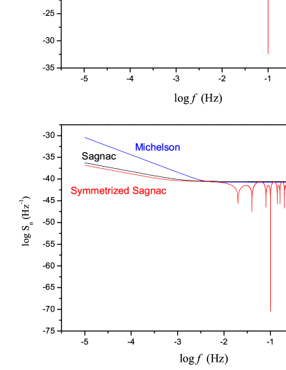
Figure 3: Top: the transfer functions $\mathcal{R}(f)$. Bottom: the noise spectrum $S_{n}(f)$.

3.3 The sensitivity of one interferometer and detection of RGW

Including the noise, the total output signal of an interferometer is a sum

$$s(t)=h_{o}(t)+n(t),$$ (46)

where $h_{o}(t)$ is the output response of (40) and $n(t)$ is a Gaussian noise signal with a zero mean $\langle n(t)\rangle=0$, uncorrelated to $h_{o}$. Define

$$\langle n(t)n(t^{\prime})\rangle=\frac{1}{2}\int^{+\infty}_{-\infty}dfe^{i2\pi f(t-t^{\prime})}S_{n}(f),$$ (47)

where $S_{n}(f)$ is the noise spectral density. It satisfies

$$\langle n^{2}(t)\rangle=\frac{1}{2}\int^{+\infty}_{-\infty}df\ S_{n}(f)=\int^{\infty}_{0}df\ S_{n}(f).$$ (48)

The noise in the frequency domain can be equivalently specified by

$$\langle\tilde{n}(f)\rangle=0,~{}~{}~{}~{}\langle\tilde{n}^{*}(f)\tilde{n}(f^{\prime})\rangle=\frac{1}{2}\delta(f-f^{\prime})S_{n}(f).$$ (49)

There are two major kinds of noise [22, 70]. The first kind is called the optical-path noise, which includes shot noise, beam pointing instabilities, thermal vibrations, etc. Among these, shot noise is the most important and its noise spectral density is given by [70]

$$S_{s}(f)=\frac{1.21\times 10^{-22}{\rm m}^{2}\,{\rm Hz}^{-1}}{(5\times 10^{9}{\rm m})^{2}}=4.84\times 10^{-42}\ {\rm Hz}^{-1}.$$ (50)

The other kind of noise is the acceleration noise with a spectral density

$$S_{a}(f)=\frac{9\times 10^{-30}{\rm m}^{2}\,{\rm s}^{-4}\,{\rm Hz}^{-1}}{(5\times 10^{9}{\rm m})^{2}(2\pi f)^{4}}=\ 2.31\times 10^{-40}\left(\frac{{\rm mHz}}{f}\right)^{4}\ {\rm Hz}^{-1}.$$ (51)

From these follow the noise spectral density of the Michelson

$$S^{m}_{n}(f)=8S_{a}(f)\left(1+\cos^{2}\left(\frac{f}{f_{*}}\right)\right)+4S_{s}(f),$$ (52)

the noise spectral density of the Sagnac

$$S_{n}^{s}(f)=6S_{s}(f)+8\left(\sin^{2}\frac{3f}{2f_{*}}+2\sin^{2}\frac{f}{2f_{*}}\right)S_{a}(f),$$ (53)

and the noise spectral density of the symmetrized Sagnac

$$S_{n}^{ss}(f)=\frac{2}{3}\left(1+2\cos\left(\frac{f}{f_{*}}\right)\right)^{2}\left(S_{s}(f)+4\sin^{2}\left(\frac{f}{2f_{*}}\right)S_{a}(f)\right).$$ (54)

These are plotted in the bottom of Fig. 3. It is seen that the noise of the Michelson is larger than those of Sagnac and symmetrized Sagnac, and the symmetrized Sagnac has the least noise. Higher symmetries in the optical path designs of Sagnac and symmetrized Sagnac cancel more noise. The symmetric Sagnac has a transfer function several orders of magnitude lower than Michelson of around $10^{-3}$ Hz, and can be used to monitor noise level in practice [88, 70].

Figure 4: The sensitivity curves $\tilde{h}(f)$ of Michelson, Sagnac and symmetrized Sagnac

To detect RGW by signals from one interferometer, one considers the auto-correlation of the total output signal

$$\langle s^{2}(t)\rangle= \langle h_{o}^{2}(t)\rangle+\langle n^{2}(t)\rangle=\int^{\infty}_{0}df\ S(f),$$ (55)

where (43) and (48) are used, and the total spectral density

$$S(f)\equiv S_{h}(f)\mathcal{R}(f)+S_{n}(f).$$ (56)

(55) is equivalently written in the frequency domain

$$\langle\tilde{s}^{*}(f)\tilde{s}(f^{\prime})\rangle=\frac{1}{2}\delta(f-f^{\prime})S(f).$$ (57)

Since both the RGW signal and noise occur in (56), SNR for a single interferometer which is denoted as SNR₁ can be naturally defined as

$$\text{SNR}_{1}\equiv\frac{h_{c}(f)}{\tilde{h}(f)},$$ (58)

where $h_{c}(f)$ is related to $S_{h}(f)$ by (38), and the sensitivity is introduced by

$$\tilde{h}(f)\equiv\sqrt{\frac{S_{n}(f)}{\mathcal{R}(f)}},$$ (59)

which reflects the detection capability of one interferometer. A smaller $\tilde{h}(f)$ indicates a better sensitivity, which requires a lower $S_{n}$ and a greater ${\mathcal{R}}$. Figure 4 shows the sensitivity curves of three interferometers, which is similar to the result of Ref.[70]. It is seen that the Michelson has the best sensitivity level, $\tilde{h}(f)\sim 10^{-20}$ Hz^-1/2 around $f_{*}=c/(2\pi L)\simeq 10^{-2}$ Hz for the arm-length $L=5\times 10^{9}$ m. This is because the transfer function $\mathcal{R}(f)$ of the Michelson is greatest, giving rise to a lowest value for $\tilde{h}(f)$, even though its $S_{n}(f)$ is slightly higher than the other two. Therefore, we shall use the Michelson in the subsequent sections. As a preliminary criterion, a single interferometer will detect RGW when SNR₁ $>1$, i.e,

$$h_{c}(f)>\tilde{h}(f).$$ (60)

This criterion was used to constrain the RGW parameters from the data of LIGO S5 [89, 79]. We plot $h_{c}(f)$ and $\tilde{h}(f)$ in Fig. 5 for a single interferometer. When the data of space-borne interferometers are available in the future, (60) will put a constraint on the parameters. The interferometer will be able to detect RGW of $\alpha_{t}>0.016$ at fixed $r=0.1$ and $\beta=-2.016$.

Figure 5: Comparison of $h_{c}(f)$ of RGW with the sensitivity $\tilde{h}(f)$ of a single interferometer.

4 Estimation of RGW spectrum by one interferometer

Now we try to determine the RGW spectrum from the output signals of one interferometer. This is a typical estimation problem of statistical signals, which can be studied by statistical methods. From the view of statistics, RGW and CMB share some similar properties, both of them form a stochastic background in the Universe, and can be modeled by a Gaussian random field [72, 73, 18].

The time series of the output signal (46) can be put into the Fourier form in frequency domain

$$\tilde{s}(f)=\tilde{h}_{o}(f)+\tilde{n}(f).$$

For practical computation, the data set can be divided into the following sample vector

$${\bf\tilde{s}}=[\tilde{s}(f_{1}),...,\tilde{s}(f_{N})],$$ (61)

with $f_{i+1}-f_{i}=\Delta f$, $i=1,2,\cdots,N$, where $N$ is a sufficiently large number. Since both $\tilde{h}_{o}(f_{i})$ and $\tilde{n}(f_{i})$, are Gaussian and independent, $\tilde{s}(f_{i})$ is a Gaussian random variable, and ${\bf\tilde{s}}$ consists of $N$ statistically independent Gaussian data points, having zero mean

$$\langle\tilde{s}(f_{i})\rangle=0.$$ (62)

The covariance matrix is (57), which is written in the discrete form

$$\Sigma_{ij}=\delta_{ij}\frac{1}{2\Delta f}\,S(f_{i}),~{}~{}~{}~{}i,j=1,2,\cdots,N$$ (63)

where the Dirac delta function $\delta(f)$ has been replaced by its discrete form [54],

$$\delta(f_{i}-f_{j})=\lim_{\Delta f\rightarrow 0}\frac{1}{\Delta f}\delta_{ij}.$$ (64)

The total spectral density in (56) is also written in the discrete form

$$S(f_{i})\equiv\left[S_{h}(f_{i})\mathcal{R}(f_{i})+S_{n}(f_{i})\right].$$ (65)

The inverse covariance matrix is

$$(\bm{\Sigma}^{-1})_{ij}=\frac{2\Delta f\delta_{ij}}{S(f_{i})}\,,$$ (66)

depending on the RGW signal $S_{h}$, the noise $S_{n}$ and the transfer function $\mathcal{R}$ of the interferometer. Note that here $\Sigma_{ij}$ is diagonal since $\tilde{s}(f_{i})$ and $\tilde{s}(f_{j})$ are independent for $i\neq j$. Given the mean and the covariance, the PDF of $\bf\tilde{s}$ is written as a multivariate Gaussian PDF [74]

$$f({\bf\tilde{s}})=\frac{1}{(2\pi)^{\frac{N}{2}}\text{det}^{\frac{1}{2}}[\bm{\Sigma}]}\exp\left\{-\frac{1}{2}{\bf\tilde{s}}\ \bm{\Sigma}^{-1}\ {\bf\tilde{s}}^{T}\right\},$$ (67)

and the likelihood function is

$$\mathcal{L}\equiv-\ln f({\bf\tilde{s}})=\frac{1}{2}\ln\text{det}[\bm{\Sigma}]+\frac{1}{2}{{\bf\tilde{s}}}\ \bm{\Sigma}^{-1}{\bf\tilde{s}}^{T}\,,$$ (68)

(dropping an irrelevant additive constant $\frac{1}{2}N\ln 2\pi$). Once the PDF is chosen, an estimator of the spectrum is a specification to give the value $S_{h}$ for the given data set $\bm{\tilde{}}s$. For this, we shall adopt the ML method. In general, $\mathcal{L}$ can be expanded in a neighborhood of some spectrum $\bar{S}_{h}(f)$,

$$\mathcal{L}= \bar{\mathcal{L}}+\sum_{k=1}^{N}\frac{\partial\mathcal{L}}{\partial S_{h}(f_{k})}(S_{h}(f_{k})-\bar{S}_{h}(f_{k}))$$

$$+\frac{1}{2}\sum_{k,\,l=1}^{N}\frac{\partial^{2}\mathcal{L}}{\partial S_{h}(f_{k})\partial S_{h}(f_{l})}\left(S_{h}(f_{k})-\bar{S}_{h}(f_{k})\right)\left(S_{h}(f_{l})-\bar{S}_{h}(f_{l})\right).$$ (69)

We look for the most likely spectrum $\bar{S}_{h}(f)$ at which $\mathcal{L}$ is minimized

$$\left.\frac{\delta\mathcal{L}}{\delta S_{h}}\right|_{\bar{S}_{h}}=0.$$ (70)

Taking the derivative of Eq. (68) with respect to $S_{h}(f_{i})$, and using the relations

$$\frac{\partial\ln\text{det}[\bm{\Sigma}]}{\partial S_{h}(f)}=\text{tr}\left(\bm{\Sigma}^{-1}\frac{\partial\bm{\Sigma}}{\partial S_{h}(f)}\right),~{}~{}~{}~{}\frac{\partial\bm{\Sigma}^{-1}}{\partial S_{h}(f)}=-\bm{\Sigma}^{-1}\frac{\partial\bm{\Sigma}}{\partial S_{h}(f)}\bm{\Sigma}^{-1},$$ (71)

one produces the first order derivative [74]

$$\frac{\partial\mathcal{L}}{\partial S_{h}(f_{i})}= \frac{1}{2}\text{tr}\left(\bm{\Sigma}^{-1}\frac{\partial\bm{\Sigma}}{\partial S_{h}(f_{i})}\right)-\frac{1}{2}\bm{\tilde{s}}\ \bm{\Sigma}^{-1}\frac{\partial\bm{\Sigma}}{\partial S_{h}(f_{i})}\bm{\Sigma}^{-1}\ \bm{\tilde{s}}^{T}\,,$$ (72)

where the zero mean of $\bm{s}$ gives no contribution to (72). From Eq. (63), one calculates

$$\frac{\partial\Sigma_{kl}}{\partial S_{h}(f_{i})}=\frac{1}{2}\frac{1}{\Delta f}\delta_{kl}\delta_{ki}\mathcal{R}(f_{k}),~{}~{}~{}~{}k,l,i=1,2,\cdots,N,$$ (73)

where

$$\frac{\partial S_{h}(f_{i})}{\partial S_{h}(f_{j})}=\delta_{ij},~{}~{}~{}~{}i,j=1,\cdots,N.$$ (74)

has been used. Substituting (63) and (73) into (72) leads to

$$\frac{\partial\mathcal{L}}{\partial S_{h}(f_{i})}= \frac{\mathcal{R}(f_{i})}{2[S(f_{i})]^{2}}\left[S_{h}(f_{i})\mathcal{R}(f_{i})+S_{n}(f_{i})-2\tilde{s}_{i}^{2}\Delta f\right].$$ (75)

Setting this to zero, one obtains the ML estimator of the RGW spectrum

$$S_{h}(f_{i})=\frac{2\Delta f}{\mathcal{R}(f_{i})}\tilde{s}_{i}^{2}-\frac{S_{n}(f_{i})}{\mathcal{R}(f_{i})},~{}~{}~{}~{}i=1,2,\cdots,N.$$ (76)

However, in practice, our knowledge is not sufficient for the spectrum $S_{n}(f_{i})$ due to noise that is actually inherent in the data [58, 88], so that the formula (76) for a single is not effective to estimate the RGW spectrum when the noise is dominantly large. In the following we turn to two detectors for estimation of RGW spectrum.

5 Cross-correlation of a pair of interferometers

5.1 The overlapping function of a pair of case for LISA

We present a pair of Michelson interferometers in space which has been studied in Refs.[69, 70]. Based on the three spacecraft forming on an equilateral triangle in Figure 2, we consider two configurations of a pair. Config. 1 consists of the three spacecraft in one triangle, but with each spacecraft carrying two sets of independent detection equipments. Then two independent Michelson interferometers form [56]: the first having the point 1 as the vertex, and the second having the point 2 as the vertex, differing from the first by a rotation of $120^{\circ}$, as in Figure 2. This configuration is economically favored, however, a possible problem is that the equipment on one craft may have dependent noise. For simplicity we assume that the noises are independent by better setup in the design. Config. 2 consists of two triangles, equipped with six spacecraft, forming two interferometers in space [69]. The second triangle is rotated $180^{\circ}$ from the first, as in Figure 6. This configuration can ensure independent noise since the six crafts are located far away from each other in space. For both configurations, we assume that the noises from the two interferometers are independent of each other, and independent of RGW.

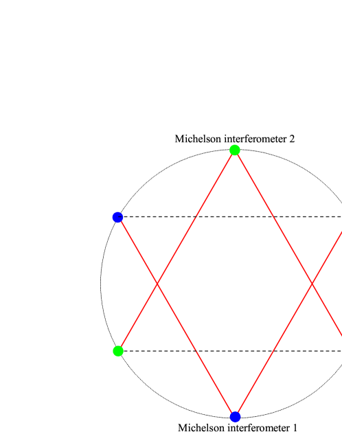
Figure 6: A pair of interferometers in two triangles for config. 2

GW signals are correlated in the two interferometers. By cross-correlating the output data of the pair, the detection capability will be enhanced. Consider the output signals from a pair of two interferometers

$$s_{1}(t) =h_{1}(t)+n_{1}(t),$$ (77)

$$s_{2}(t) =h_{2}(t)+n_{2}(t),$$ (78)

each is similar to Eq. (46). It is assumed that

$$\langle h_{i}(t)n_{j}(t)\rangle=0,~{}~{}~{}~{}~{}~{}\langle n_{1}(t)n_{2}(t)\rangle=0,$$ (79)

and

$$\langle n^{2}_{1}(t)\rangle=\int_{0}^{\infty}dfS_{n1}(f),~{}~{}~{}~{}~{}~{}\langle n^{2}_{2}(t)\rangle=\int_{0}^{\infty}dfS_{n2}(f),$$ (80)

where $S_{n1}$, $S_{n2}$ are the noise spectral densities of the two interferometer as in (48), and specified as in Eq. (52) for the Michelson. When the two interferometers are identical, one can take $S_{n1}\simeq S_{n2}$.

Using the output response of (39) for each interferometer and formula (35), the ensemble average of the correlation of two output responses is

$$\langle h_{1}(t)h_{2}(t^{\prime})\rangle= \frac{1}{2}\int_{-\infty}^{+\infty}dfS_{h}(f)\int\frac{d\hat{\Omega}}{4\pi}\sum_{A=\times,+}F_{1}^{A*}(\hat{\Omega},f)F_{2}^{A}(\hat{\Omega},f)e^{-i2\pi f\hat{\Omega}\cdot(\mathbf{r}_{1}-\mathbf{r}_{2})}e^{i2\pi f(t-t^{\prime})}$$

$$= \int_{0}^{\infty}dfS_{h}(f)\mathcal{R}_{12}(f)e^{i2\pi f(t-t^{\prime})},$$ (81)

similarly, by (41) and (35),

$$\langle\tilde{h}_{1}(f)\tilde{h}_{2}(f^{\prime})\rangle= \frac{1}{2}\delta(f-f^{\prime})S_{h}(f)\mathcal{R}_{12}(f),$$ (82)

where the transfer function $\mathcal{R}_{12}(f)$ is

$$\mathcal{R}_{12}(f)\equiv\int\frac{d\hat{\Omega}}{4\pi}\sum_{A=\times,+}F_{1}^{A*}(\hat{\Omega},f)F_{2}^{A}(\hat{\Omega},f)e^{-i2\pi f\hat{\Omega}\cdot(\mathbf{r}_{1}-\mathbf{r}_{2})},$$ (83)

where $\mathbf{r}_{1}$ and $\mathbf{r}_{2}$ represent the respective positions of the vertices of the two interferometers. A higher value of $\mathcal{R}_{12}(f)$ means a better capability to transfer incoming RGW into signals from the detector.

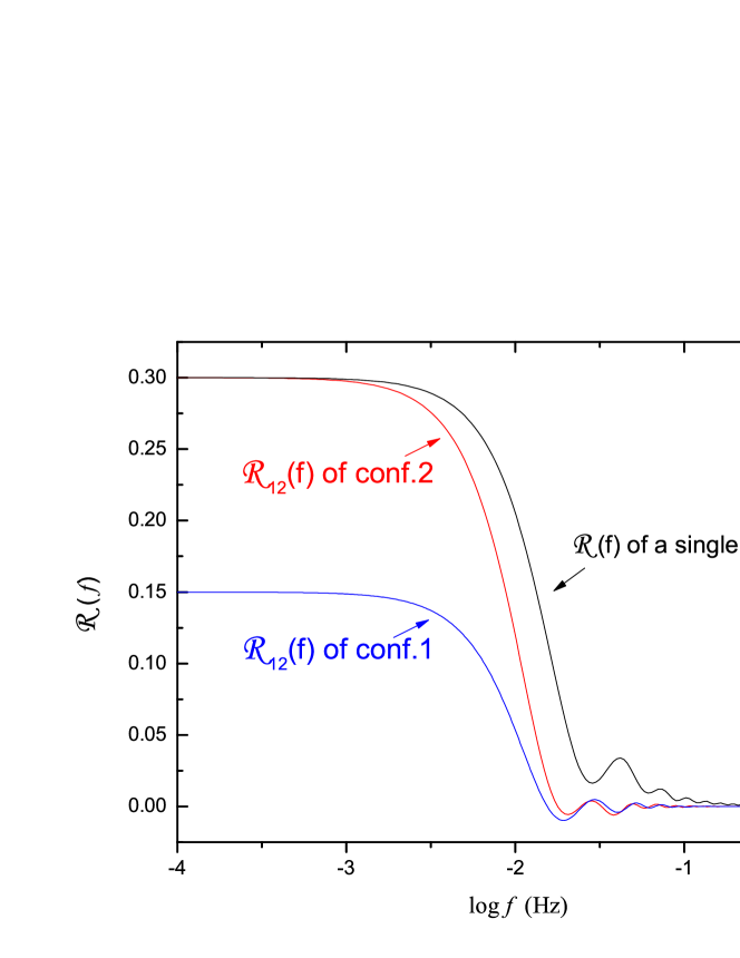
Figure 7: A comparison between the transfer function of a single and a pair.

In Fig. 7 we plot the transfer function of a single and of a pair with conf.1 and conf.2. One introduces the overlapping reduction function $\gamma(f)$ [58, 59] by normalizing $\mathcal{R}_{12}(f)$ as the following

$$\gamma(f)\equiv\frac{5}{\sin^{2}\beta_{0}}\mathcal{R}_{12}(f)=\frac{20}{3}\mathcal{R}_{12}(f).~{}~{}~{}~{}{\rm for~{}conf.1}$$ (84)

$$\gamma(f)\equiv\frac{5}{2\sin^{2}\beta_{0}}\mathcal{R}_{12}(f)=\frac{10}{3}\mathcal{R}_{12}(f).~{}~{}~{}~{}{\rm for~{}conf.2}$$ (85)

where $\beta_{0}=\pi/3$ is the angle between arms of one interferometer, $\sin^{2}\beta_{0}=3/4$. Clearly, $\gamma(f)$ depends on the geometry of the pair, and transfers the incident RGW from all the directions (by integration over angle $\hat{\Omega}$) into the output signal. We compute $\gamma(f)$ numerically and plot it in Fig. 8 for config.1 (top) and config.2 (bottom). At high frequencies, $\gamma(f)$ oscillates around zero. At low frequencies, $\gamma(f)\rightarrow 1$ for both configurations. To a high accuracy, it can be fitted by the following formula

$$\gamma(f)=\left\{\begin{array}[]{ll}1-0.811508\left(\frac{f}{f_{*}}\right)^{2}+0.241292\left(\frac{f}{f_{*}}\right)^{4}-0.0374118\left(\frac{f}{f_{*}}\right)^{6},&f<f_{*}\\ 0.43636+2.12337\left(\frac{f}{f_{*}}\right)-4.00143\left(\frac{f}{f_{*}}\right)^{2}+2.37321\left(\frac{f}{f_{*}}\right)^{3}\\ \hskip 125.19194pt-0.588745\left(\frac{f}{f_{*}}\right)^{4}+0.0528759\left(\frac{f}{f_{*}}\right)^{5},&f_{*}\leq f<3.3f_{*}\\ 0.000311254-0.11762e^{-0.37176f/f_{*}}\bigg{[}0.0849126\\ \hskip 73.97733pt-\sin\bigg{(}2.89649-2.40829\left(\frac{f}{f_{*}}\right)e^{0.00978685f/f_{*}}\bigg{)}\bigg{]},&3.3f_{*}\leq f\end{array}\right.$$ (86)

for the config. 1, and

$$\gamma(f)=\left\{\begin{array}[]{ll}1-\frac{383}{504}\left(\frac{f}{f_{*}}\right)^{2}+\frac{893}{3888}\left(\frac{f}{f_{*}}\right)^{4}-\frac{5414989}{143700480}\left(\frac{f}{f_{*}}\right)^{6},&f<f_{*}\\ 0.629524+1.52435\left(\frac{f}{f_{*}}\right)-3.23303\left(\frac{f}{f_{*}}\right)^{2}+1.96633\left(\frac{f}{f_{*}}\right)^{3}\\ \hskip 125.19194pt-0.496608\left(\frac{f}{f_{*}}\right)^{4}+0.0454382\left(\frac{f}{f_{*}}\right)^{5},&f_{*}\leq f<3.3f_{*}\\ 0.000190192-0.157835e^{-0.570049f/f_{*}}\bigg{[}0.264226\par\\ \hskip 73.97733pt-\sin\bigg{(}1.66131-2.01502\left(\frac{f}{f_{*}}\right)e^{0.0349379f/f_{*}}\bigg{)}\bigg{]},&3.3f_{*}\leq f\end{array}\right.$$ (87)

for config.2. $\gamma(f)$ of configs. 1 and 2 look the same except around $f\simeq(2\sim 8)\times 10^{-2}$ Hz. Formula (87) at $f<f_{*}$ agrees with that in Ref.[69], which does not list the expression for the part $f>f_{*}$. See also Ref.[61]. In the following we shall mainly use config. 2 for demonstration.

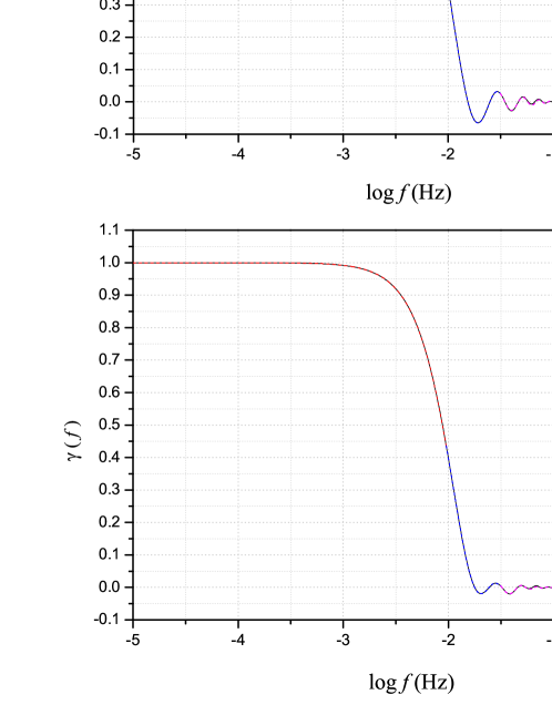
Figure 8: The overlap reduction function for a pair. Top: Config.1; Bottom: Config.2. Solid lines are plotted numerically and dotted lines by the fitted formulae (86) and (87).

5.2 SNR for a pair case for LISA

To suppress the noise of a pair, one defines the cross-correlated, integrated signal of $s_{1}(t)$ and $s_{2}(t^{\prime})$ as the following [59]

$$C \equiv\int_{-T/2}^{T/2}dt\int_{-\infty}^{+\infty}dt^{\prime}s_{1}(t)s_{2}(t^{\prime})Q(t-t^{\prime})$$

$$=\int_{-\infty}^{\infty}df\int_{-\infty}^{\infty}df^{\prime}\delta_{T}(f-f^{\prime})\tilde{s}_{1}^{\,*}(f)\tilde{s}_{2}(f^{\prime})\tilde{Q}(f^{\prime}),$$ (88)

where $T$ is the observation time, $\tilde{s}(f)=\tilde{s}(-f)$ is the Fourier transform of $s(t)$ and $\tilde{s}^{\,*}_{1}(f)=\tilde{s}_{1}(-f)$, $Q(t-t^{\prime})$ is a filter function to be determined by maximizing SNR₁₂ (SNR for the pair), its Fourier transform is $\tilde{Q}(f)=\tilde{Q}(-f)$, and

$$\delta_{T}(f)\equiv\int_{-T/2}^{T/2}dt\,e^{-i2\pi ft}=\frac{\sin(\pi fT)}{\pi f},$$ (89)

is the finite-time Dirac delta function. For a finite $T$, one has $\delta_{T}(0)=T$, and in the limit $T\rightarrow\infty$, $\delta_{T}(f)$ reduces to the Dirac delta function $\delta(f)$. Given the frequency band of $(10^{-4}-10^{-1})$ Hz, one can take the length of each segment, say, $T\simeq 3$ hours$\sim 10^{4}$ s. When $T$ is large enough, $\delta_{T}(\Delta f)$ is sharply peaked over a narrow region of width $\sim 1/T$. Thus, in the integration (5.2), the product of $\tilde{s}^{*}(f)\tilde{s}(f^{\prime})$ contributes only in the region of $|f-f^{\prime}|<1/T\sim 10^{-4}$ Hz. The frequency band contains $\sim 10^{3}$ of these regions. By the central limit theorem, $C$ is well-approximated by a Gaussian random variable.

In actual computations, the cross-correlated signal $C$ can be expressed either in the time domain, or equivalently, the frequency domain. In the following we shall use the frequency domain. By Eqs. (79) and (82), the mean of $C$ is

$$\mu=\langle C\rangle= \int_{-T/2}^{T/2}df\int_{-\infty}^{\infty}df^{\prime}\delta_{T}(f-f^{\prime})\langle\tilde{s}_{1}^{*}(f)\tilde{s}_{2}(f^{\prime})\rangle\tilde{Q}(f^{\prime})$$

$$= \frac{3T}{10}\int_{0}^{\infty}dfS_{h}(f)\gamma(f)\tilde{Q}(f).$$ (90)

Notice that the mean $\mu$ is non-zero, in contrast to (62) for one interferometer. Furthermore, the noise terms disappear in the above since they are removed by cross-correlation, and only the RGW signal accumulates with the observation time $T$. This feature of a pair is the advantage over a single case. A greater value of $\mu$ is desired for RGW detection. The covariance $C$ is

$$\sigma^{2}= \langle C^{2}\rangle-\langle C\rangle^{2}$$ (91)

$$= \int_{-\infty}^{\infty}df\int_{-\infty}^{\infty}df^{\prime}\int_{-\infty}^{\infty}dk\int_{-\infty}^{\infty}dk^{\prime}\delta_{T}(f-f^{\prime})\delta_{T}(k-k^{\prime})\tilde{Q}(f^{\prime})\tilde{Q}^{*}(k^{\prime})$$

$$\times\left\langle\left[\tilde{h}_{1}^{*}(f)+\tilde{n}_{1}^{*}(f)\right]\left[\tilde{h}_{2}(f^{\prime})+\tilde{n}_{2}(f^{\prime})\right]\left[\tilde{h}_{1}(k)+\tilde{n}_{1}(k)\right]\left[\tilde{h}^{*}_{2}(k^{\prime})+\tilde{n}^{*}_{2}(k^{\prime})\right]\right\rangle$$

$$-\bigg{(}\int_{-\infty}^{\infty}df\int_{-\infty}^{\infty}df^{\prime}\delta_{T}(f-f^{\prime})\frac{1}{2}\delta(f-f^{\prime})S_{h}(f^{\prime})\mathcal{R}_{12}(f)\tilde{Q}(f^{\prime})\bigg{)}^{2}.$$ (92)

Using the “factorization” property [59]

$$\langle x_{1}x_{2}x_{3}x_{4}\rangle=\langle x_{1}x_{2}\rangle\langle x_{3}x_{4}\rangle+\langle x_{1}x_{3}\rangle\langle x_{2}x_{4}\rangle+\langle x_{1}x_{4}\rangle\langle x_{2}x_{3}\rangle\,,$$

valid for Gaussian random variables $x_{1},x_{2},x_{3},x_{4}$, each having zero mean, and using Eqs. (42), (79) and (82), one obtains

$$\sigma^{2}= \frac{1}{4}\int_{-\infty}^{\infty}df\int_{-\infty}^{\infty}df^{\prime}\delta^{2}_{T}(f-f^{\prime})\left|\tilde{Q}(f^{\prime})\right|^{2}\Big{[}S_{1n}(f)S_{2n}(f^{\prime})+\mathcal{R}(f^{\prime})S_{h}(f^{\prime})S_{1n}(f)$$

$$+\mathcal{R}(f)S_{h}(f)S_{2n}(f^{\prime})+\mathcal{R}(f)S_{h}(f)\mathcal{R}(f^{\prime})S_{h}(f^{\prime})+\mathcal{R}_{12}(f)S_{h}(f)\mathcal{R}_{12}(f^{\prime})S_{h}(f^{\prime})\Big{]},$$ (93)

where $\mathcal{R}(f)$ is the transfer function for a single case in (44), and $\mathcal{R}_{12}(f)$ is the transfer function for a pair in (83). For $T$ sufficiently long, one $\delta_{T}(f-f^{\prime})$ can be set to be the Dirac function $\delta(f-f^{\prime})$, yielding

$$\sigma^{2}=\frac{T}{2}\int_{-\infty}^{\infty}df\,|\tilde{Q}(f)|^{2}\,M(f)\,,$$ (94)

where the function

$$M(f)\equiv S_{1n}(f)S_{2n}(f)+\mathcal{R}(f)\Big{[}S_{1n}(f)+S_{2n}(f)\Big{]}S_{h}(f)+\Big{[}\mathcal{R}^{2}(f)+\mathcal{R}_{12}^{2}(f)\Big{]}S_{h}^{2}(f),$$ (95)

which reduces to

$$M(f)\simeq S^{2}_{n}(f)+2\mathcal{R}(f)S_{h}(f)S_{n}(f)+\left[\mathcal{R}^{2}(f)+\mathcal{R}_{12}^{2}(f)\right]S_{h}^{2}(f)$$ (96)

when $S_{1n}\simeq S_{2n}=S_{n}$. We plot the functions $M$, $S^{2}_{n}$, and $\left(\mathcal{R}^{2}+\mathcal{R}_{12}^{2}\right)S_{h}^{2}$ of (96) for different values of parameters in Figs.9 with SNR₁₂ given by (101). $M$ is dominated by $S^{2}_{n}$ at reasonable values of SNR₁₂, so that one can take $M(f)\simeq S_{1n}(f)S_{2n}(f)$ as a good approximation.

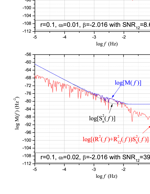
Figure 9: $M$, $S^{2}_{n}$, $\left(\mathcal{R}^{2}+\mathcal{R}_{12}^{2}\right)S_{h}^{2}$. Top: for SNR${}_{12}=8.62$; Bottom: for SNR${}_{12}=395$.

The SNR of the pair is defined as [59]

$$\text{SNR}_{12}=\frac{\mu}{\sigma}=\frac{3\sqrt{T}}{10}\frac{\int_{0}^{\infty}dfS_{h}(f)\gamma(f)\tilde{Q}(f)}{\left[\int_{0}^{\infty}df\,|\tilde{Q}(f)|^{2}M(f)\right]^{1/2}},$$ (97)

which describes the detection capability of a pair. To maximize $\text{SNR}_{12}$, one chooses the filter function [59]

$$\tilde{Q}(f)=\frac{S_{h}(f)\gamma(f)}{M(f)},$$ (98)

for which the mean is

$$\mu=\frac{3T}{10}\int_{0}^{\infty}df\frac{S^{2}_{h}(f)\,\gamma^{2}(f)}{M(f)},$$ (99)

the covariance is

$$\sigma^{2}=\frac{T}{2}\int_{0}^{\infty}df\frac{S^{2}_{h}(f)\,\gamma^{2}(f)}{M(f)}=\frac{5}{3}\mu\,,$$ (100)

and

$$\text{SNR}_{12}=\frac{3\sqrt{2T}}{10}\left[\int_{0}^{\infty}df\frac{\gamma^{2}(f)S_{h}^{2}(f)}{M(f)}\right]^{1/2}.$$ (101)

$\text{SNR}_{12}\propto r$ for large noise, and its dependences on $\beta$ and $\alpha_{t}$ are shown in Fig. 10.

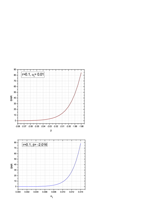
Figure 10: SNR₁₂ changes with $\beta$ (top) and $\alpha_{t}$ (bottom).

When the noise is dominant, Eq. (99) becomes

$$\mu=\frac{3T}{10}\int_{0}^{\infty}df\frac{S^{2}_{h}(f)\,\gamma^{2}(f)}{S_{1n}(f)S_{2n}(f)}\,,$$ (102)

(101) becomes

$$\text{SNR}_{12} =\frac{3\sqrt{2T}}{10}\left[\int_{0}^{\infty}df\frac{\gamma^{2}(f)S_{h}^{2}(f)}{S_{1n}(f)S_{2n}(f)}\right]^{1/2}.$$ (103)

Formula (103) is similar to that of the ground-based LIGO [59, 58, 69]. Clearly, the dependence of SNR₁₂ on $r$, $\beta$ and $\alpha_{t}$ is implicitly contained in $S_{h}(f)$, and SNR${}_{12}\propto r$ for large noise. There is a growing factor $\sqrt{T}$ of $\text{SNR}_{12}$ in (103), because the noise gets suppressed by cross-correlation and only the RGW signals accumulate with time.

To demonstrate the capability of a pair of space interferometers to detect RGW, we compute the values of SNR₁₂ using Eq. (101). The result is in Table 1, with an observation time $T=1$ year and $r=0.1$. For comparison, we have also attached the result for the pair of ground-based LIGO S6 [30, 31] and LIGO O1 and Advanced LIGO as well [2], for which we use the formulae of $\text{SNR}_{12}$ and $\gamma(f)$ in Ref.[59]. It is seen that SNR₁₂ of LISA is higher than that of Advanced LIGO by 4 orders of magnitude for the default $(\alpha_{t}=0,\beta=-2)$, and by 5 orders of magnitude for the observed-inferred $(\alpha_{t}=0,\beta=-2.016)$. Therefore, LISA will have a much stronger capability than LIGO to detect RGWs.

Table 1: SNR₁₂ for a pair case for LISA and for a pair case for LIGO with $r=0.1$.

$\alpha_{t},\beta$	-0.005, -2.05	0, -2.016	0, -2	0.005, -1.95	0.01, -1.9
LIGO S6	$1.6\times 10^{-13}$	$5.0\times 10^{-10}$	$2.2\times 10^{-9}$	$3.1\times 10^{-5}$	$4.2\times 10^{-1}$
LIGO O1	$3.0\times 10^{-11}$	$7.3\times 10^{-8}$	$3.0\times 10^{-7}$	$3.0\times 10^{-3}$	$3.1\times 10^{1}$
Advanced LIGO	$3.3\times 10^{-10}$	$7.3\times 10^{-7}$	$2.9\times 10^{-6}$	$2.7\times 10^{-2}$	$2.5\times 10^{2}$
A pair case for LISA	$1.1\times 10^{-4}$	$2.2\times 10^{-2}$	$6.8\times 10^{-2}$	$3.8\times 10^{1}$	$4.9\times 10^{2}$

5.3 The sensitivity of a pair compared with a single

To describe the sensitivity of a pair, we can extend the expression of (103) and allow SNR₁₂ to vary with frequency. Consider the averaged SNR₁₂ over a frequency band of width $\Delta f$, centered at $f$ as the following [70]

$$\text{SNR}_{12}(f) \simeq\sqrt{T}\left[\int_{f-\Delta f/2}^{f+\Delta f/2}df\frac{\mathcal{R}_{12}^{2}(f)S_{h}^{2}(f)}{\left(S_{n}(f)\right)^{2}}\right]^{1/2}$$

$$\simeq\sqrt{T}\sqrt{\Delta f}\,S_{h}(f)\,\overline{\left(\frac{\mathcal{R}_{12}^{2}(f)}{\left(S_{n}(f)\right)^{2}}\right)}^{\,1/2}\,.$$ (104)

In analogy to (59), we define the effective sensitivity of the pair

$$\tilde{h}_{12}(f)\equiv\sqrt{\frac{S_{h}(f)}{\text{SNR}_{12}(f)}}=\frac{1}{(T\Delta f)^{1/4}}\overline{\left(\frac{\mathcal{R}_{12}^{2}(f)}{\left(S_{n}(f)\right)^{2}}\right)}^{\ -1/4},$$ (105)

which depends on $T$ and frequency resolution $\Delta f$, in contrast to that of a single in (59). A longer $T$ increases the sensitivity of (105). The sensitivities of a single and a pair are plotted in Fig. 11, where $\Delta f=f/10$ and $T=1$ year are taken. Clearly, a pair has a better sensitivity than a single by $\sim 100$ times around $f\sim 10^{-2}$ Hz.

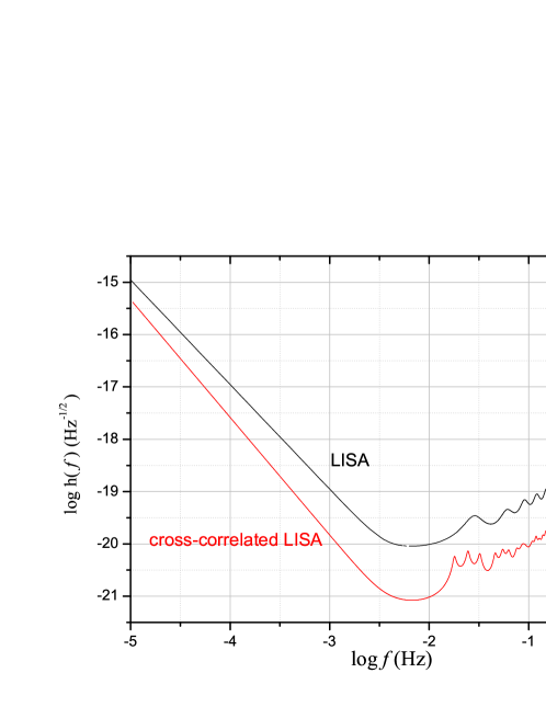
Figure 11: The sensitivity curves of a single and a pair.

5.4 Constraints on the RGW parameters by a pair

By (103), a constraint on SNR₁₂ will transfer into a constraint on ($r$, $\beta$, $\alpha_{t}$). One such a constraint on SNR₁₂ is given by [59]

$$\text{SNR}_{12}\geq\sqrt{2}\left(\text{erfc}^{-1}(2\alpha)-\text{erfc}^{-1}(2\gamma)\right),$$ (106)

where $\text{erfc}^{-1}(\alpha)$ is the inverse function of the complementary error function $\text{erfc}(z)\equiv\frac{2}{\sqrt{\pi}}\int_{z}^{\infty}dx\ e^{-x^{2}}$, $\alpha$ is called the false alarm rate, and $\gamma$ is called the detection rate. Taking $\alpha=5\%$ and $\gamma=95\%$, Eq. (106) gives

$$\text{SNR}_{12}\geq 3.29.$$ (107)

Thus, fixing two parameters out of $(r,\alpha_{t},\beta)$, we can convert (107) into a lower limit on the remaining parameter of RGW. Table 2 shows the lower limits of $\alpha_{t}$ with the other two being fixed for $T=1$ year.

Table 2: The lower limits of $\alpha_{t}$ with the other two being fixed.

	-1.94	-1.96	-1.98	-2	-2.02	-2.04	-2.06	-2.08
0.1	-0.00041	0.00190	0.00421	0.00653	0.00884	0.01115	0.01346	0.01577
0.05	0.00074	0.00306	0.00537	0.00768	0.00999	0.01230	0.01461	0.01692

6 Estimation by integrated signals from a pair

6.1 The integrated output signals

We now try to determine the RGW spectrum by a pair. Let the sample vector of the cross-correlated signals

$$\bm{C}=[C_{1},C_{2},...,C_{N}],$$ (108)

where each $C_{i}$ is the cross-correlated, integrated output signal of (5.2),

$$C_{i}=\int_{-\infty}^{\infty}df\int_{-\infty}^{\infty}df^{\prime}\delta_{T_{i}}(f-f^{\prime})\tilde{s}_{1}^{\,*}(f)\tilde{s}_{2}(f^{\prime})\tilde{Q}(f^{\prime}),~{}~{}~{}~{}i=1,2,\cdots,N,$$ (109)

and $N$ is the number of segments, and is sufficiently large. When $T\gg$ the light travel time $L/c\sim 2$ seconds between the two detectors of LISA, non-overlapping $C_{i}$ and $C_{j}$ for $j\neq i$ are statistically independent [59]. For each $i$, $C_{i}$ has the mean $\mu_{i}=\left\langle C_{i}\right\rangle$ given by (99), and the variance $\sigma^{2}_{i}=\langle C_{i}^{2}\rangle-\mu_{i}^{2}$ given by (100). In general, $\mu_{i}$ varies for different $i$, so does $\sigma^{2}_{i}$. Denote the mean of $\bm{C}$ by $\bm{\mu}=[\mu_{1},\mu_{2},...,\mu_{N}]$, and the covariance matrix by $\bm{\Sigma}=\left(\Sigma_{ij}\right)$ with

$$\Sigma_{ij}=\left\langle(C_{i}-\mu_{i})(C_{j}-\mu_{j})\right\rangle\,,~{}~{}~{}~{}i,j=1,2,\cdots,N,$$ (110)

which is diagonal, $\Sigma_{ij}=\delta_{ij}\sigma_{j}^{2}$, by independence. (Here $\bm{\Sigma}$ for a pair should not be confused with that in Section 4 for a single.) Explicitly,

$$\mu_{i}=\langle C_{i}\rangle=\frac{3T_{i}}{10}m,$$ (111)

$$\Sigma_{ij}=\delta_{ij}\,b\mu_{j},$$ (112)

where $b\equiv 5/3$ and

$$m\equiv\int_{0}^{\infty}df\frac{S^{2}_{h}(f)\,\gamma^{2}(f)}{M(f)}$$ (113)

is a functional of $S_{h}(f)$. We assume that the PDF of $\bf C$ is a multivariate Gaussian

$$f({\bf C})=\frac{1}{(2\pi)^{\frac{N}{2}}\text{det}^{\frac{1}{2}}[\bm{\Sigma}]}\exp\left\{-\frac{1}{2}{(\bm{C}-\bm{\mu})}\ \bm{\Sigma}^{-1}\ \left(\bm{C}-\bm{\mu}\right)^{T}\right\}\,,$$ (114)

which, by (112), is

$$f({\bf C})=\frac{1}{(2\pi)^{\frac{N}{2}}\,(\Pi_{i}^{N}b\mu_{i})^{\frac{1}{2}}}\exp\left\{-\frac{1}{2b}\sum_{i}^{N}{\frac{\left(C_{i}-\mu_{i}\right)^{2}}{\mu_{i}}}\right\}\,.$$ (115)

The likelihood function is, after dropping an irrelevant constant $\frac{1}{2}N\ln 2\pi$,

$$\mathcal{L}\equiv-\ln f=\frac{1}{2}\sum_{i}^{N}\ln(b\mu_{i})+\frac{1}{2b}\sum_{i}^{N}{\frac{\left(C_{i}-\mu_{i}\right)^{2}}{\mu_{i}}},$$ (116)

which is a functional of the spectrum $S_{h}$ through $\mu_{i}$. Once the PDF is chosen, an estimator of the spectrum is a specification to give the value $S_{h}$ for the given data set $\bf C$. For this, we shall adopt the ML method. In general, $\mathcal{L}$ can be expanded in a neighborhood of some spectrum $\bar{S}_{h}(f)$,

$$\mathcal{L}= \bar{\mathcal{L}}+\sum_{k=1}^{N}\frac{\partial\mathcal{L}}{\partial S_{h}(f_{k})}(S_{h}(f_{k})-\bar{S}_{h}(f_{k}))$$

$$+\frac{1}{2}\sum_{k,\,l=1}^{N}\frac{\partial^{2}\mathcal{L}}{\partial S_{h}(f_{k})\partial S_{h}(f_{l})}\left(S_{h}(f_{k})-\bar{S}_{h}(f_{k})\right)\left(S_{h}(f_{l})-\bar{S}_{h}(f_{l})\right).$$ (117)

We look for the most likely spectrum $\bar{S}_{h}(f)$ at which $\mathcal{L}$ is minimized

$$\left.\frac{\delta\mathcal{L}}{\delta S_{h}}\right|_{\bar{S}_{h}}=0.$$ (118)

The first order derivative is (see Appendix A for details)

$$\frac{\delta\mathcal{L}}{\delta S_{h}}= \frac{1}{2}\sum^{N}_{l}\bigg{[}\frac{1}{\mu_{l}}-\frac{C^{2}_{i}}{b\mu_{i}^{2}}+\frac{1}{b}\bigg{]}\frac{\delta\mu_{l}}{\delta S_{h}}$$

$$= \frac{1}{2}\frac{S_{h}(f)\,\gamma^{2}(f)}{M(f)}\left(1-\frac{N(f)}{M(f)}\right)\left(\frac{N}{m}-\frac{2}{m^{2}}\sum^{N}_{i}\frac{C^{2}_{i}}{T_{i}}+\frac{1}{2b^{2}}\sum^{N}_{i}T_{i}\right),$$ (119)

where $\,m$ is given by (113) and $N(f)$ is given by (A.9). The analytical expression of the solution for (118) is not available, and one needs to use numerical methods. The Newton-Raphson method [73, 18, 75] is generally used to find the ML-estimate of the spectrum. In many applications, the Newton-Raphson method is known to converge quadratically in the neighborhood of the root. For instance, in the spectral estimation of CMB anisotropies [73, 18], typically 3-4 iterations will be sufficient. Let $S^{(0)}_{h}(f)$ be a trial power spectrum, which can be tentatively chosen as the analytical spectrum (38) with some values of parameters. In the neighborhood of $S^{(0)}_{h}(f)$, the first order derivative of the likelihood is expanded as the following

$$\frac{\delta\mathcal{L}}{\delta S_{h}(f)}\bigg{|}_{S_{h}(f)}\simeq\frac{\delta\mathcal{L}}{\delta S_{h}(f)}\bigg{|}_{S^{(0)}_{h}(f)}+\int df^{\prime}\frac{\delta^{2}\mathcal{L}}{\delta S_{h}(f)\delta S_{h}(f^{\prime})}\bigg{|}_{S^{(0)}_{h}(f)}\left(S_{h}(f^{\prime})-S^{(0)}_{h}(f^{\prime})\right)=0.$$ (120)

As an approximation, $\frac{\delta^{2}\mathcal{L}}{\delta S_{h}\delta S_{h}}$ is replaced by its expected value, i.e, the Fisher matrix,

$$\mathcal{F}(f,f^{\prime}) =\left[\frac{S_{h}(f^{\prime})\,\gamma^{2}(f^{\prime})}{M(f^{\,{}^{\prime}})}\left(1-\frac{N(f^{\prime})}{M(f^{\prime})}\right)\right]\left[\frac{S_{h}(f)\,\gamma^{2}(f)}{M(f)}\left(1-\frac{N(f)}{M(f)}\right)\right]\frac{1}{2}\left(\frac{N}{m^{2}}+\frac{9}{25m}\sum_{l}^{N}T_{l}\right),$$ (121)

(see Appendix A for the derivation). However, this Fisher matrix is degenerate and has no inverse, and one will not be able to invert Eq.(120) to get an estimated spectrum. This is because the signal $C_{i}$ constructed in (109) is an integration over frequency, as is $\mu_{i}$. On the other hand, for spectrum estimation, one needs to assign a value $S_{h}(f_{j})$ at each frequency $f_{j}$. Thus, we conclude that $C_{i}$ will not help to estimate the RGW spectrum by a pair, even though it is useful for detection of an RGW signal.

6.2 Parameter estimation in a Bayesian approach

We shall be able to use $C_{i}$ to estimate one parameter of RGW in a Bayesian approach. Consider the PDF as in Eq. (115),

$$f({\bf C};\bm{\theta})=\frac{1}{(2\pi)^{\frac{N}{2}}\,(\Pi_{i}^{N}b\mu_{i}(\bm{\theta}))^{\frac{1}{2}}}\exp\left\{-\frac{1}{2b}\sum_{i}^{N}{\frac{\left(C_{i}-\mu_{i}(\bm{\theta})\right)^{2}}{\mu_{i}(\bm{\theta})}}\right\}\,,$$ (122)

where $\bm{\mu}(\theta)$ and $\bm{\Sigma}(\bm{\theta})$ as in (111) and (112) respectively now depend on the RGW parameters through the theoretical spectrum $S_{h}$, and $\bm{\theta}$ denotes the RGW parameters which are random variables since they are some functions of the data set [74]. We adopt the unbiased estimation, which assumes that the average value of an estimator of the parameters $\bm{\theta}$ is regarded as its true value. Using the ML method, the likelihood function $\mathcal{L}=-\ln f(\bm{\theta})$ can also be Taylor expanded around certain values $\bm{\bar{\theta}}$

$$\mathcal{L}=\bar{\mathcal{L}}+\sum_{a}\frac{\partial\mathcal{L}}{\partial\theta_{a}}\bigg{|}_{\bm{\bar{\theta}}}\,(\theta_{a}-\bar{\theta}_{a})+\frac{1}{2}\sum_{a,b}\,\frac{\partial^{2}\mathcal{L}}{\partial\theta_{a}\partial\theta_{b}}\bigg{|}_{\bm{\bar{\theta}}}(\theta_{a}-\bar{\theta}_{a})(\theta_{b}-\bar{\theta}_{b})+\,\cdots\,.$$

Now we require $\bm{\bar{\theta}}$ to be the ML estimator, at which

$$\frac{\partial\mathcal{L}}{\partial\theta_{a}}\,\bigg{|}_{\bm{\bar{\theta}}}=0,~{}~{}~{}~{}a=1,2,3.$$ (123)

As is known [74], when $N$ is large enough, the second order derivative at $\bm{\bar{\theta}}$ is equal to its average value,

$$\mathcal{F}_{ab}\equiv\bigg{\langle}\frac{\partial^{2}\mathcal{L}}{\partial\theta_{a}\partial\theta_{b}}\,\bigg{|}_{\bm{\bar{\theta}}}\bigg{\rangle}=\frac{\partial^{2}\mathcal{L}}{\partial\theta_{a}\partial\theta_{b}}\bigg{|}_{\bm{\bar{\theta}}},~{}~{}~{}~{}a,b=1,2,3,$$

so that in the neighborhood of $\bm{\bar{\theta}}$, the PDF of (122) becomes the following Bayesian PDF in the parameter space

$$f(\bm{\theta})\propto\exp{[-\mathcal{L}]}\propto\exp\left[-\frac{1}{2}(\bm{\theta}-\bm{\bar{\theta}}){\bf\mathcal{F}}(\bm{\theta}-\bm{\bar{\theta}})^{T}\right]\,,$$ (124)

which is approximately Gaussian in a neighborhood of $\bm{\bar{\theta}}$. For detailed derivation see appendix 7B of Ref.[74].

The likelihood function follows (122) as

$$\mathcal{L}(\bm{C};\bm{\theta})\equiv-\ln f({\bf C};\bm{\theta})=\frac{1}{2}\sum_{i}^{N}\ln\left(b\mu_{i}(\bm{\theta})\right)+\frac{1}{2b}\sum_{i}^{N}{\frac{\left(C_{i}-\mu_{i}(\bm{\theta})\right)^{2}}{\mu_{i}(\bm{\theta})}}.$$ (125)

To estimate $\bm{\theta}$, one needs the first order derivative (See Appendix A),

$$\frac{\partial\mathcal{L}}{\partial\theta_{a}}= \int df\frac{S_{h}(f)\,\gamma^{2}(f)}{M(f)}\left(1-\frac{N(f)}{M(f)}\right)\frac{\partial S_{h}(f)}{\partial\theta_{a}}\left(\frac{N}{m}-\frac{2}{m^{2}}\sum^{N}_{i}\frac{C^{2}_{i}}{T_{i}}+\frac{1}{2b^{2}}\sum^{N}_{i}T_{i}\right),$$ (126)

and the $3\times 3$ Fisher matrix

$$\mathcal{F}_{ab}= \left(\int_{0}^{\infty}df^{\prime}\frac{S_{h}(f^{\prime})\,\gamma^{2}(f^{\prime})}{M(f^{\prime})}\left(1-\frac{N(f^{\prime})}{M(f^{\prime})}\right)\,\frac{\partial S_{h}(f^{\prime})}{\partial\theta_{a}}\right)$$

$$\times\left(\int_{0}^{\infty}df\frac{S_{h}(f)\,\gamma^{2}(f)}{M(f)}\left(1-\frac{N(f)}{M(f)}\right)\,\frac{\partial S_{h}(f)}{\partial\theta_{b}}\right)2\left(\frac{N}{m^{2}}+\frac{9}{25m}\sum_{i}^{N}T_{i}\right)\,.$$ (127)

However, this Fisher matrix is degenerate and has no inverse. Thus, one can not determine the whole set $(r,\beta,\alpha_{t})$ simultaneously. What one can do is to estimate only one of the RGW parameters, while the other two parameters are fixed at certain values, or marginalized. Note that this method can not determine the correlation between two parameters, which will be given by another method in Section 8.3 later. For the former case, one gets the conditional PDF, and for the latter, one integrates the PDF of (122) over $\theta_{b}$ and $\theta_{c}$, and gets the marginal PDF for $\theta_{a}$

$$f({\bf C};\theta_{a})\equiv\int\int f({\bf C};\bm{\theta})d\theta_{b}d\theta_{c}$$ (128)

and the marginal likelihood function $\mathcal{L}(\bm{C};\theta_{a})\equiv-\ln f({\bf C};\theta_{a})$. With these specifications, one can estimate the parameter $\theta_{a}$. Let $\theta^{(0)}_{a}$ be a trial parameter. We expand the first order derivative of $\mathcal{L}$, conditional or marginalizing, around $\theta^{(0)}_{a}$

$$\frac{\partial\mathcal{L}}{\partial\theta_{a}}\bigg{|}_{\bm{\theta}}\simeq\frac{\partial\mathcal{L}}{\partial\theta_{a}}\bigg{|}_{\bm{\theta}^{(0)}}+\frac{\partial^{2}\mathcal{L}}{\partial\theta_{a}\partial\theta_{a}}\bigg{|}_{\bm{\theta}^{(0)}}\left(\theta_{a}-\theta_{a}^{(0)}\right)=0.$$ (129)

Replacing $\frac{\partial^{2}\mathcal{L}}{\partial\theta_{a}\partial\theta_{a}}$ by the $(aa)$ element of Fisher matrix $\mathcal{F}_{aa}\equiv\left\langle\frac{\partial^{2}}{\partial\theta_{a}\partial\theta_{a}}\mathcal{L}\right\rangle$, one gets

$$\theta_{a}=\theta_{a}^{(0)}-\mathcal{F}_{aa}^{-1}\frac{\partial\mathcal{L}}{\partial\theta_{a}}\,\bigg{|}_{\bm{\theta}^{(0)}}.$$ (130)

By iteration, one will obtain the estimate of $\theta_{a}$. This is a general formula to estimate one parameter. The Fisher matrix $\mathcal{F}_{ab}$ also gives the standard error of the estimated parameter. When the data sample is sufficiently large, one can take the equality in the Cramer-Rao lower bound [74]

$$\sigma^{2}_{\theta_{a}}=\mathcal{F}^{-1}_{aa}(f)$$ (131)

where $\mathcal{F}^{-1}_{aa}$ is evaluated at the ML-estimate parameter $\theta_{a}$ that has been obtained.

In fact, when noise is dominant over the RGW signal, the estimate of $r$ can be also obtained analytically. By the property $\,m\propto r^{2}$ implied by (113), one can write $\,m(r)=r^{2}m(r=1)$ with $\beta$ and $\alpha_{t}$ being fixed in $\,m(r=1)$. Setting (6.1) to zero, and solving for $\,m$, one has the positive root

$$\bar{m}= \frac{25}{9}\frac{1}{\frac{1}{N}\sum_{i}^{N}T_{i}}\left(-1+\sqrt{1+\frac{36}{25}\frac{1}{N^{2}}\left(\sum_{j}^{N}T_{j}\right)\left(\sum_{i}^{N}\frac{C_{i}^{2}}{T_{i}}\right)}\right)\,,$$ (132)

from which one obtains the analytical ML-estimate of $r$ as the following

$$r=\frac{1}{\sqrt{m(r=1)}}\sqrt{\frac{25/9}{\frac{1}{N}\sum_{i}^{N}T_{i}}\left(-1+\sqrt{1+\frac{36}{25N^{2}}\left(\sum_{j}^{N}T_{j}\right)\sum_{i}^{N}\frac{C_{i}^{2}}{T_{i}}}\right)}\,.$$ (133)

However, no analytical ML-estimates are available for $\beta$ and $\alpha_{t}$. Still one can estimate $\beta$ and $\alpha_{t}$ in a manner simpler than (130). Let $\theta_{a}$ be $\beta$ and

$$\mathcal{M}[\theta_{a}]\equiv\int_{0}^{\infty}df\frac{S^{2}_{h}(f)\,\gamma^{2}(f)}{M(f)}-\bar{m}=0,$$ (134)

in which $r$ and $\alpha_{t}$ are fixed. We use the Newton-Raphson method by iterations as before. Write $\mathcal{M}[\theta_{a}]$ as

$$\mathcal{M}[\theta_{a}]\simeq\mathcal{M}[\theta_{a}^{(0)}]+\frac{\partial\mathcal{M}}{\partial\theta_{a}}\bigg{|}_{\theta_{a}^{(0)}}\,\left(\theta_{a}-\theta^{(0)}_{a}\right)=0,$$ (135)

where $\theta^{(0)}_{a}$ is a trial value and

$$\frac{\partial\mathcal{M}}{\partial\theta_{a}}=\int_{0}^{\infty}df\frac{2S_{h}(f)\,\gamma^{2}(f)}{M(f)}\left(1-\frac{N(f)}{M(f)}\right)\,\frac{\partial S_{h}(f)}{\partial\theta_{a}}.$$ (136)

One solves (135) and gets the estimate

$$\theta_{a}=\theta_{a}^{(0)}-\frac{\partial\mathcal{M}}{\partial\theta_{a}}\bigg{|}_{\theta_{a}^{(0)}}^{-1}\,\mathcal{M}[\theta_{a}^{(0)}].$$ (137)

Similarly, the estimation of $\alpha_{t}$ can be also done. Note that since the filter function $\hat{Q}$ in (98) contains the theoretical spectrum $S_{h}(f)$, this ML-estimation method is essentially a technique of matched filter [90].

We perform a numerical simulation to estimate $r$, using (130). For $r=0.1$, $\alpha_{t}=0.016$ and $\beta=-2.016$ with SNR₁₂=179, we use the PDF (115) to generate cross-correlated data stream numerically. We take $T\simeq 3$ hours $\sim$$10^{4}$ s for one segment, with total observation duration $\sim 1$ year, and number of segments $n\sim 3\times 10^{3}$. Then we estimate $r$ numerically by (130), and after five steps of iteration, $r$ converges to $r_{ML}=0.1011$.

According to (124) and (131), the standard deviation is $\sigma_{\theta_{a}}\equiv 1/\sqrt{\mathcal{F}_{aa}}$. If the estimation is required to be at the $95\%$ confidence level (cl), $0.95=\frac{2}{\sqrt{\pi}}\int_{0}^{\Delta\theta_{a}/(\sqrt{2}\sigma_{\theta_{a}})}e^{-t^{2}}dt$, the resolution of the estimated parameter $\theta_{a}$ will be

$$\Delta\theta_{a}=1.96\sigma_{\theta_{a}}\ \ {\rm\ at\ }95\%\,\,{\rm cl}\,.$$ (138)

Table 3 lists the resolution of $r$, $\alpha_{t}$ and $\beta$, separately, and the corresponding values of SNR₁₂ ($\geq 3.29$).

Table 3: Resolution of $r$, $\alpha_{t}$ and $\beta$ separately at $95\%$ cl for a pair

$r$	$\alpha_{t}$	$\beta$	$\Delta r/r$	$\Delta\alpha_{t}$	$\Delta\beta$	SNR12
0.05	0.01	-2.016	$2.58\times 10^{-2}$	$4.29\times 10^{-5}$	$3.72\times 10^{-4}$	4.36
0.05	0.015	-2.016	$1.46\times 10^{-2}$	$2.42\times 10^{-5}$	$2.10\times 10^{-4}$	72.8
0.1	0	-1.93	$2.56\times 10^{-2}$	$4.28\times 10^{-5}$	$3.70\times 10^{-4}$	8.34
0.1	0.01	-2.016	$2.55\times 10^{-2}$	$4.26\times 10^{-5}$	$3.69\times 10^{-4}$	8.62
0.1	0.01	-1.93	$1.46\times 10^{-2}$	$2.40\times 10^{-5}$	$2.09\times 10^{-4}$	390
0.1	0.016	-2.016	$9.72\times 10^{-3}$	$1.61\times 10^{-5}$	$1.40\times 10^{-4}$	179

7 Spectral estimation by ensemble average of a pair

To estimate the RGW spectrum, we turn to the method of ensemble averaging of data from a pair. Consider the output signals $\tilde{s}_{1}(f)$, $\tilde{s}_{2}(f)$ in frequency space from (77) and (78) respectively. Since the noises are uncorrelated, the ensemble average $\left\langle s_{1}(f)\tilde{s}_{2}(f^{\prime})\right\rangle$ is given by (82). In practice, when there are $n$ independent sets of observational data, each being $(s_{1}(f)\tilde{s}_{2}(f^{\prime}))_{i}$, they can form the sample mean,

$$\left\langle s_{1}(f)\tilde{s}_{2}(f^{\prime})\right\rangle_{t}\equiv\frac{(s_{1}(f)\tilde{s}_{2}(f^{\prime}))_{1}+\cdots+(s_{1}(f)\tilde{s}_{2}(f^{\prime}))_{n}}{n}\,,$$ (139)

which represents the ensemble average when the independent sets of data are large enough. Thus (82) becomes

$$\langle\tilde{s}_{1}(f)\tilde{s}_{2}(f^{\prime})\rangle_{t}=\frac{1}{2}\delta(f-f^{\prime})S_{h}(f)\mathcal{R}_{12}(f).$$ (140)

In practical analysis, we can replace $\delta(f-f^{\prime})$ by its discrete form in (64),

$$\langle\tilde{s}_{1}(f_{i})\tilde{s}_{2}(f_{j})\rangle_{t}=\frac{\delta_{ij}}{2\Delta f}S_{h}(f_{i})\mathcal{R}_{12}(f_{i}).$$ (141)

Solving Eq. (141), one obtains an estimate of the RGW spectrum by a pair

$$\bar{S}_{h}(f_{i})=\frac{2\Delta f}{\mathcal{R}_{12}(f_{i})}\left\langle\tilde{s}_{1}(f_{i})\tilde{s}_{2}(f_{i})\right\rangle_{t}.$$ (142)

(142) is the main formula in our paper to estimate the spectrum from a pair. As an advantage, it does not require a priori knowledge of the noise spectrum, in contrast to (76). In the ensemble averaging method, $\langle\tilde{s}_{1}(f_{i})\tilde{s}_{2}(f_{j})\rangle_{t}$ as the basic quantity does not involve integration over frequency.

Using (142), we conduct a numerical simulation to examine its feasibility. First, we construct the vector of RGW output response ${\bf\tilde{h}_{o}}(f_{i})\equiv[\tilde{h}_{1}(f_{i}),\tilde{h}_{2}(f_{i})]$ with $i=1,2,\cdots,N$, where each of $\tilde{h}_{1}(f_{i})$ and $\tilde{h}_{2}(f_{i})$ is defined as in Eq. (41). The mean and variance are given in Eqs. (42) and (82), and the corresponding PDF is

$$f\left({\bf\tilde{h}_{o}}(f_{i})\right)=\frac{1}{(2\pi)^{\frac{N}{2}}\text{det}^{\frac{1}{2}}[\bm{\Sigma}_{(h)}(f_{i})]}\exp\left\{-\frac{1}{2}{\bf\tilde{h}_{o}}(f_{i})\left[\bm{\Sigma}_{(h)}(f_{i})\right]^{-1}\left[{\bf\tilde{h}_{o}}(f_{i})\right]^{T}\right\},\ i=1,2,\cdots,N\ ,$$ (143)

where the covariance matrix is

$$\bm{\Sigma}_{(h)}(f_{i})\equiv\frac{1}{2\Delta f}S_{h}(f_{i})\left(\begin{array}[]{cc}\mathcal{R}(f_{i})_{1}&\mathcal{R}_{12}(f_{i})\\ \mathcal{R}_{12}(f_{i})&\mathcal{R}(f_{i})_{2}\\ \end{array}\right),\ i=1,2,\cdots,N\ .$$ (144)

Here $\mathcal{R}(f_{i})_{1}$ and $\mathcal{R}(f_{i})_{2}$ are transfer function of the interferometer $1$ and $2$ respectively, and we can assume $R_{1}\simeq R_{2}$, and $\mathcal{R}_{12}$ is the transfer function for the pair defined in (83). The inverse matrix of (144) is

$$[\bm{\Sigma}_{(h)}(f_{i})]^{-1}=\frac{2\Delta f}{S_{h}(f_{i})}\frac{1}{\mathcal{R}^{2}(f_{i})-\mathcal{R}_{12}^{2}(f_{i})}\left(\begin{array}[]{cc}\mathcal{R}(f_{i})&-\mathcal{R}_{12}(f_{i})\\ -\mathcal{R}_{12}(f_{i})&\mathcal{R}(f_{i})\\ \end{array}\right)\ .$$ (145)

Similarly, for the noise in the pair, we write the noise vector ${\bf\tilde{n}}(f_{i})\equiv[\tilde{n}_{1}(f_{i}),\tilde{n}_{2}(f_{i})]$. The mean and covariance are in (49) and (80), and the PDF is

$$f\left({\bf\tilde{n}}(f_{i})\right)=\frac{1}{(2\pi)^{\frac{N}{2}}\text{det}^{\frac{1}{2}}[\bm{\Sigma}_{(n)}(f_{i})]}\exp\left\{-\frac{1}{2}{\bf\tilde{n}}(f_{i})\left[\bm{\Sigma}_{(n)}(f_{i})\right]^{-1}\left[{\bf\tilde{n}}(f_{i})\right]^{T}\right\}\ ,$$ (146)

where the covariance matrix is

$$\bm{\Sigma}_{(n)}(f_{i})\equiv\frac{S_{n}(f_{i})}{2\Delta f}\left(\begin{array}[]{cc}1&0\\ 0&1\\ \end{array}\right)\ ,$$ (147)

which is diagonal since the noises in the pair are uncorrelated. Based on the above construction, the joint PDF for the total output signal is given by (67) with the covariance matrix $\bm{\Sigma}(f_{i})=\bm{\Sigma}_{(h)}(f_{i})+\bm{\Sigma}_{(n)}(f_{i})$.

We use PDFs (143) and (146) to numerically generate the output response and noise of a pair. We need the data set of $n$ segments $({\bf\tilde{s}}(f_{i}))_{1},\cdots,({\bf\tilde{s}}(f_{i}))_{n}$. One can take one typical segment of the data stream with a period of $T\simeq 3$ hours $\sim$$10^{4}$ s, with total observation duration $\sim 1$ year, and number of segments $n\sim 3\times 10^{3}$. According to the PDF of (143) and (146) with the specific variance $\bm{\Sigma}$ by taking RGW with $r=0.1$, $\alpha_{t}=0.016$, $\beta=-2.016$ with SNR${}_{12}=179$, we numerically generate $3\times 10^{3}$ independent sets of random data streams ${\bf\tilde{s}}(f_{i})$ ($i=1,\cdots,N$). Substituting these generated data streams into Eq. (142), we obtain the estimated RGW spectrum $\bar{S}_{h}(f_{i})$ for $n=30$ and $n=3000$, as shown in Fig. 12. For illustration, the theoretical spectrum and the simulated noise are also shown. The estimation depends on the length of simulated data. A longer length $n$ of data gives a better estimate. In an ideal case of infinitely long data length, the off-diagonal elements of the covariance matrix for practical noise signal would be 0, and the RGW signal at all relevant frequencies could be detected. But with a finite size of data, the estimation will be limited when the noise is large. As Fig. 12 shows, the estimate (142) at high frequencies is actually contributed by the nonzero off-diagonal elements of noise, i.e, $\bar{S}_{h}(f)\sim$$\frac{2\Delta f\langle\tilde{n}_{1}(f_{i})\tilde{n}_{2}(f_{i})\rangle}{\mathcal{R}_{12}(f_{i})}$ at $f>10^{-2}$ Hz, because of a finite length of data.

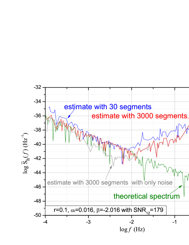
Figure 12: The estimated spectrum by a pair. The cases with only the theoretical spectrum and simulated noise are also shown.

8 Estimations by correlation of un-integrated signals from a pair

In this section, we adopt a method of correlation of un-integrated signals to estimate the spectrum and parameters of RGW as suggested by Ref. [76]. By dividing the whole frequency range of the data into many small segments, the mean value of the correlation variable over each segment is taken as the representative point for the segment. As an approximation, the method is able to give the estimate of the RGW spectrum, as well as the three parameters of RGW, improving that in Section 6. We assume that the output data are sufficient for this purpose.

8.1 A correlation variable of un-integrated signals

In analogy with (3.4) in Ref. [76], we divide a positive frequency range into $N$ segments, and the $i$-th segment $F_{i}$ $(i=1,2,...,N)$ of width $\delta f_{i}$ has a center frequency $f_{i}$. For instance, the frequency range is taken as $(10^{-4}\sim 1)$ Hz for LISA, $N\sim 10^{4}$, and $\delta f\sim 10^{-4}$ Hz. A correlation variable is defined in each segment $F_{i}$ as

$$Z_{i}\equiv\sum_{f\in F_{i}}\Delta f\,\tilde{s}^{*}_{1}(f)\tilde{s}_{2}(f),\,\,\,i=1,2,...,N$$ (148)

where the frequency resolution $\Delta f=1/T_{1}\ll\delta f_{i}$ with $T_{1}$ being the observation period, say $\Delta f\sim 10^{-6}$ Hz, so that each segment contains a large number of Fourier modes. (Notice that (3.4) in Ref.[76] should have a factor of $\Delta f$ for consistency of dimension.) The mean of $Z_{i}$ is

$$\mu_{i}=\langle Z_{i}\rangle=\sum_{f\in F_{i}}\Delta f\frac{1}{2}\delta(f-f)S_{h}(f)\mathcal{R}_{12}(f),$$ (149)

where (79) and (82) are used. Using the formula (64) to replace the Dirac delta function by its discrete form, (149) can be written as the following

$$\mu_{i}=\sum_{f\in F_{i}}\Delta f\frac{1}{2\Delta f}S_{h}(f)\mathcal{R}_{12}(f).$$ (150)

The summation can be approximately replaced as

$$\mu_{i}=\frac{\delta f_{i}}{2\Delta f}S_{h}(f_{i})\mathcal{R}_{12}(f_{i}),\,\,\,i=1,2,...,N$$ (151)

where $S_{h}(f_{i})\mathcal{R}_{12}(f_{i})$ is the mean value over the $i$-th segment, as suggested in Ref. [76]. To keep the error small in this approximation, $\delta f_{i}$ should be sufficiently small so that the mean value of the function represents the summation function within $\delta f_{i}$. (We note that the overlapping reduction function $\gamma_{12}(f)$ defined in Ref. [76] is related to our $\mathcal{R}_{12}(f)$ by $\gamma_{12}(f)=\frac{5}{2}\mathcal{R}_{12}(f)$, which together with (38) leads to $\mu_{i}=\frac{\delta f_{i}}{\Delta f}\frac{3H_{0}^{2}}{20\pi^{2}}\frac{\Omega_{g}(f)}{f^{3}}\gamma_{12}(f)$, the same as (3.5) in Ref. [76].)

The variance of $Z_{i}$ is

$$\sigma_{i}^{2}=\left\langle\Big{(}Z_{i}-\langle Z_{i}\rangle\Big{)}^{2}\right\rangle=\langle Z_{i}^{2}\rangle-\langle Z_{i}\rangle^{2}.$$ (152)

By noting that $\int_{-\infty}^{+\infty}df^{\prime}\delta(f-f^{\prime})$ is equivalent to $2\sum_{f^{\prime}\in F_{j}}\Delta f\delta(f-f^{\prime})$, (148) can be written as

$$Z_{i}=\sum_{f\in F_{i}}\Delta f\left[2\sum_{f^{\prime}\in F_{j}}\Delta f\delta(f-f^{\prime})\right]\tilde{s}^{*}_{1}(f)\tilde{s}_{2}(f^{\prime}),$$ (153)

and the variance is written as

$$\sigma_{i}^{2} =4\left\langle\sum_{f\in F_{i}}\Delta f\sum_{f^{\prime}\in F_{j}}\Delta f\delta(f-f^{\prime})\tilde{s}^{*}_{1}(f)\tilde{s}_{2}(f^{\prime})\sum_{k\in F_{i}}\Delta f\sum_{k^{\prime}\in F_{j}}\Delta f\delta(k-k^{\prime})\tilde{s}^{*}_{1}(k)\tilde{s}_{2}(k^{\prime})\right\rangle-\mu_{i}^{2}\,.$$ (154)

By similar calculations leading to (94), we obtain the following result

$$\sigma_{i}^{2}=\frac{1}{8}\frac{\delta f_{i}}{\Delta f}M(f_{i}),\,\,\,i=1,2,...,N$$ (155)

where $M(f)$ is defined in (95). For large noise, $M(f)\simeq S_{1n}(f)S_{2n}(f)$,

$$\sigma_{i}^{2}\simeq\frac{1}{8}\frac{\delta f_{i}}{\Delta f}S_{1n}(f_{i})S_{2n}(f_{i}),$$ (156)

which is the same as (3.6) in Ref. [76].

SNR of each segment for this correlation is defined as [76]

$$\text{SNR}^{2}_{i}\equiv\frac{\mu_{i}^{2}}{\sigma_{i}^{2}}=2\frac{\delta f_{i}}{\Delta f}\frac{\mathcal{R}_{12}^{2}(f_{i})S_{h}^{2}(f_{i})}{M(f_{i})},$$ (157)

and summing up all segments yields the total SNR

$$\text{SNR}^{2}_{\text{C}}=2\sum_{i=1}^{N}\frac{\delta f_{i}}{\Delta f}\frac{\mathcal{R}_{12}^{2}(f_{i})S_{h}^{2}(f_{i})}{M(f_{i})}.$$ (158)

Replacing $\Delta f$ with $1/T_{1}$, the summation $\sum_{i=1}^{N}\delta f$ with integration $\int_{0}^{\infty}df$, one has the SNR over an observation period $T_{1}$ as

$$\text{SNR}_{\text{C}}=\sqrt{2T_{1}}\left[\int_{0}^{\infty}df\frac{\mathcal{R}_{12}^{2}(f)S_{h}^{2}(f)}{M(f)}\right]^{1/2}.$$ (159)

When the whole observation duration $T$ consists of many observation periods, we can use $T$ to replace $T_{1}$ in the above formula. This result is consistent with (101) by noting that $\mathcal{R}_{12}(f)=\frac{3}{10}\gamma(f)$.

8.2 Spectrum estimation

Since $\delta f_{i}/\Delta f\gg 1$, according to the central limit theorem, $Z_{i}$ can be described by a Gaussian distribution, and the PDF for ${\bf Z}\equiv[Z_{1},Z_{2},...,Z_{N}]$ is

$$f({\bf Z})=\frac{1}{(2\pi)^{\frac{N}{2}}\,(\Pi_{i}^{N}\sigma_{i}^{2})^{\frac{1}{2}}}\exp\left\{-\frac{1}{2}\sum_{i}^{N}{\frac{\left(Z_{i}-\mu_{i}\right)^{2}}{\sigma_{i}^{2}}}\right\}\,.$$ (160)

The likelihood functional is, after dropping an irrelevant constant $\frac{1}{2}N\ln 2\pi$,

$$\mathcal{L}\equiv-\ln f({\bf Z})=\frac{1}{2}\sum_{i}^{N}\ln(\sigma_{i}^{2})+\frac{1}{2}\sum_{i}^{N}{\frac{\left(Z_{i}-\mu_{i}\right)^{2}}{\sigma_{i}^{2}}},$$ (161)

which is a functional of the spectrum $S_{h}$ through $\mu_{i}$. We look for the most likely power spectrum $\bar{S}_{h}$ at which $\frac{\partial\mathcal{L}}{\partial S_{h}}\big{|}_{\bar{S}_{h}}=0$. The first order derivative is

$$\frac{\partial\mathcal{L}}{\partial S_{h}(f_{j})}=\frac{1}{2}\sum_{i}^{N}\bigg{[}\frac{1}{\sigma_{i}^{2}}\frac{\partial\sigma_{i}^{2}}{\partial S_{h}(f_{j})}-\frac{\left(Z_{i}-\mu_{i}\right)^{2}}{(\sigma_{i}^{2})^{2}}\frac{\partial\sigma_{i}^{2}}{\partial S_{h}(f_{j})}-\frac{2\left(Z_{i}-\mu_{i}\right)}{\sigma_{i}^{2}}\frac{\partial\mu_{i}}{\partial S_{h}(f_{j})}\bigg{]}.$$ (162)

Plugging (151) and (155) into the above, by $\frac{\partial S_{h}(f_{i})}{\partial S_{h}(f_{j})}=\delta_{ij}$, one has

$$\frac{\partial\mathcal{L}}{\partial S_{h}(f_{i})}=\frac{N(f_{i})}{S_{h}(f_{i})M(f_{i})}-\frac{8\left(Z_{i}-(\frac{\delta f_{i}}{2\Delta f}S_{h}(f_{i})\mathcal{R}_{12}(f_{i}))\right)^{2}}{\frac{\delta f_{i}}{\Delta f}S_{h}(f_{i})\left[M(f_{i})\right]^{2}}N(f_{i})-\frac{4\mathcal{R}_{12}(f_{i})\left(Z_{i}-(\frac{\delta f_{i}}{2\Delta f}S_{h}(f_{i})\mathcal{R}_{12}(f_{i}))\right)}{M(f_{i})},$$ (163)

where $N(f)$ is defined in (A.9). In the neighborhood of a trial spectrum $S^{(0)}_{h}(f)$, the first order derivative is expanded as the following

$$\frac{\partial\mathcal{L}}{\partial S_{h}(f_{i})}\bigg{|}_{S_{h}(f_{i})}\simeq\frac{\partial\mathcal{L}}{\partial S_{h}(f_{i})}\bigg{|}_{S^{(0)}_{h}(f_{i})}+\sum_{k=1}^{N}\frac{\partial^{2}\mathcal{L}}{\partial S_{h}(f_{i})\partial S_{h}(f_{k})}\bigg{|}_{S^{(0)}_{h}(f)}\left(S_{h}(f_{k})-S^{(0)}_{h}(f_{k})\right)=0.$$ (164)

As an approximation, $\frac{\partial^{2}\mathcal{L}}{\partial S_{h}\partial S_{h}}$ is replaced by its expected value, i.e, the Fisher matrix which by a formula similar to (A.5) is given by

$$F_{ij}=\left\langle\frac{\partial^{2}\mathcal{L}}{\partial S_{h}(f_{i})\partial S_{h}(f_{j})}\right\rangle= \sum_{k,l=1}^{N}\frac{\partial\mu_{k}}{\partial S_{h}(f_{i})}\frac{\delta_{kl}}{\sigma_{k}^{2}}\frac{\partial\mu_{l}}{\partial S_{h}(f_{j})}+\frac{1}{2}\sum_{k,l,m,r=1}^{N}\left(\frac{\delta_{kl}}{\sigma_{k}^{2}}\delta_{lm}\frac{\partial(\sigma_{l}^{2})}{\partial S_{h}(f_{i})}\frac{\delta_{mr}}{\sigma_{m}^{2}}\delta_{rk}\frac{\partial(\sigma_{r}^{2})}{\partial S_{h}(f_{j})}\right).$$ (165)

Substituting (151) and (155) into the above yields

$$F_{ij}= \left[\frac{\delta f_{i}}{\Delta f}\frac{2\mathcal{R}_{12}^{2}(f_{i})}{M(f_{i})}+\frac{2N^{2}(f_{i})}{S^{2}_{h}(f_{i})M^{2}(f_{i})}\right]\delta_{ij}.$$ (166)

It is remarked that the Fisher matrix is not degenerate, in contrast to (121) which is degenerate. In the approximation of large noise, one has $M(f)\simeq S_{1n}(f)S_{2n}(f)$, $N(f)=\frac{1}{2}S_{h}(f)\frac{\partial{M(f)}}{\partial S_{h}(f)}\simeq 0$, and (166) reduces to that used in Ref.[76]

$$F_{ij}\simeq \left[\frac{\delta f_{i}}{\Delta f}\frac{2\mathcal{R}_{12}^{2}(f_{i})}{S_{1n}(f_{i})S_{2n}(f_{i})}\right]\delta_{ij}.$$ (167)

We plot $F_{ii}(f)$ of (166) and of (167) in Fig.13. They differ significantly at high frequencies. Thus, we shall use the full expression (166) in computations later.

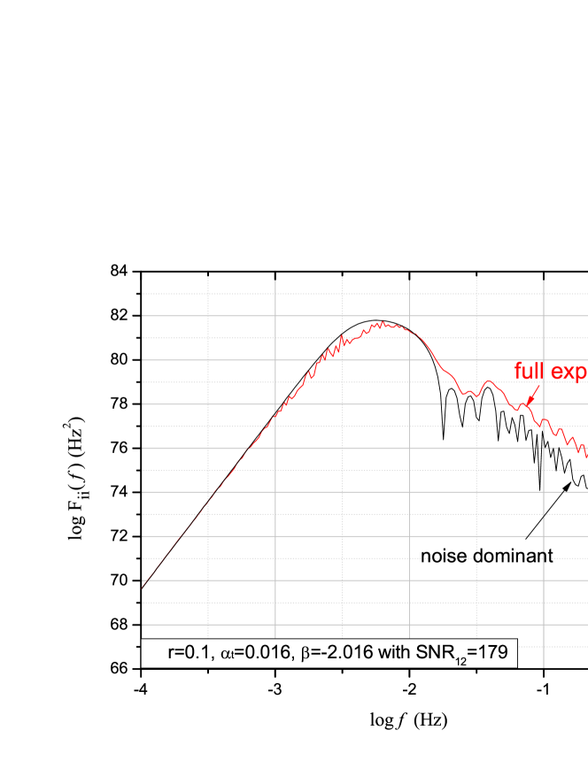
Figure 13: The diagonal element $F_{ii}$ to estimate spectrum for both the full expression (166) and the noise dominant (167) cases.

Given $F_{ij}$, one solves Eq.(164) for the estimated spectrum

$$S_{h}(f_{i})=S^{(0)}_{h}(f_{i})-\sum_{j=1}^{N}(F^{\,-1})_{ij}\frac{\partial\mathcal{L}}{\partial S_{h}(f_{j})}\bigg{|}_{S^{(0)}_{h}}.$$ (168)

To avoid random outcomes from one set of datastream, similar to (139), we shall replace $\frac{\partial\mathcal{L}}{\partial S_{h}(f_{k})}$ by its sample mean in practical computation

$$S_{h}(f_{i})=S^{(0)}_{h}(f_{i})-\left(\frac{\delta f_{i}}{\Delta f}\frac{2\mathcal{R}_{12}^{2}(f_{i})}{M(f_{i})}+\left.\frac{2N^{2}(f_{i})}{S^{2}_{h}(f_{i})M^{2}(f_{i})}\right)^{-1}\left\langle\frac{\partial\mathcal{L}}{\partial S_{h}(f_{i})}\right\rangle_{t}\right|_{S^{(0)}_{h}}\,,$$ (169)

where the expression (166) has been used. This equation will be used to estimate the spectrum of RGW numerically by Newton-Raphson iteration [73, 18, 75].

We perform a simulation to estimate $S_{h}(f)$. We divide a one-year duration into 100 periods, which are regarded as $n=100$ realizations of data output. Thus, one observation period $T_{1}\simeq 1$year$/100\simeq 3.2\times 10^{5}$s. The working frequency range $(10^{-4}\sim 1)$ Hz is divided into $N\simeq 10637$ segments and the width of each segment is $\delta f\simeq 9.4\times 10^{-5}$ Hz. Thus, each segment contains $\delta f/\Delta f\simeq 30$ frequency points. For RGW we take $r=0.1$, $\alpha_{t}=0.016$ and $\beta=-2.016$, and the formula (159) yields SNR${}_{C}=179$. We numerically generate the output response $[\tilde{h}_{1,1}(f_{i}),\cdots,\tilde{h}_{1,\,n}(f_{i});\tilde{h}_{2,1}(f_{i}),\cdots,\tilde{h}_{2,\,n}(f_{i})]$ according to (143) and the noise $[\tilde{n}_{1,1}(f_{i}),\cdots,\tilde{n}_{1,\,n}(f_{i});\tilde{n}_{2,1}(f_{i}),\cdots,\tilde{n}_{2,\,n}(f_{i})]$ according to (146) of a pair, for $i=1,\cdots,10637$ and for $n=100$ realizations. We use Eq. (148) to calculate the correlated signal $[Z_{i,1},\cdots,Z_{i,\,n}]$ for $n=100$ realizations. Using these generated data streams, we apply Newton-Raphson iteration to Eq. (169) to estimate the spectrum of RGW numerically. Fig. 14 shows the resulting estimator of spectrum $S_{h}^{(n)}(f)$ after each iterative step. It is seen that after three iterations, $S_{h}^{(n)}(f)$ converges. The estimated RGW spectrum $\bar{S}_{h}(f_{i})$ is shown in in Fig. 15. For illustration, the theoretical spectrum is also shown. It is seen that the rapid oscillations in the estimated spectrum are smoother than the theoretical one. This is because the estimated spectrum is actually a mean $\sim\frac{1}{\delta f_{i}}\sum_{f\in F_{i}}\Delta f$ in each segment in this method.

We compare the correlation method in this section with the ensemble averaging method of Section 7. Firstly, the correlation method uses the average value as the representative for each segment, and losses some fine information about the RGW spectrum. Secondly, this method needs more computing time by the iteration for each frequency point. However, this method can estimate the parameters directly as in the following subsection whereas the ensemble averaging method can not.

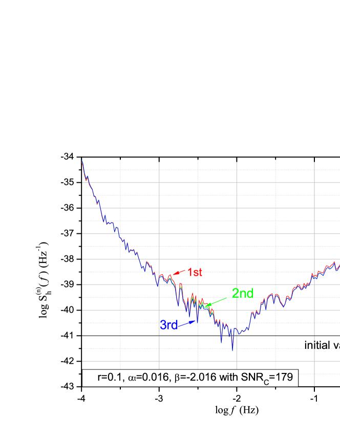
Figure 14: The estimator of spectrum $S_{h}^{(n)}(f)$ in each iterative step for a pair.

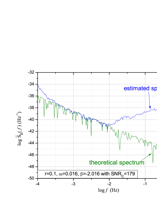
Figure 15: The estimated spectrum by the correlation method for a pair. The theoretical spectrum is also shown.

8.3 Parameter estimation

Now we estimate parameters of RGW by using the correlated data stream $Z_{\,i}$ in a Bayesian approach. Consider the PDF as in Eq. (160),

$$f({\bf Z};\bm{\theta})=\frac{1}{(2\pi)^{\frac{N}{2}}\,(\Pi_{i}^{N}\sigma_{i}^{2}(\bm{\theta}))^{\frac{1}{2}}}\exp\left\{-\frac{1}{2}\sum_{i}^{N}{\frac{\left(Z_{i}-\mu_{i}(\bm{\theta})\right)^{2}}{\sigma_{i}^{2}(\bm{\theta})}}\right\}\,,$$ (170)

where $\mu_{i}(\bm{\theta})$ and $\sigma_{i}^{2}(\bm{\theta})$ given by (151) and (155) respectively, are now regarded as functions of parameters $\bm{\theta}$ through the theoretical spectrum $S_{h}(f)$. The likelihood function $\mathcal{L}=-\ln f(\bm{\theta})$ can also be Taylor expanded around certain values $\bm{\bar{\theta}}$

$$\mathcal{L}=\bar{\mathcal{L}}+\sum_{a}\frac{\partial\mathcal{L}}{\partial\theta_{a}}\bigg{|}_{\bm{\bar{\theta}}}\,(\theta_{a}-\bar{\theta}_{a})+\frac{1}{2}\sum_{a,b}\,\frac{\partial^{2}\mathcal{L}}{\partial\theta_{a}\partial\theta_{b}}\bigg{|}_{\bm{\bar{\theta}}}(\theta_{a}-\bar{\theta}_{a})(\theta_{b}-\bar{\theta}_{b})+\,\cdots\,.$$

Now we require $\bm{\bar{\theta}}$ to be the ML estimator, at which

$$\frac{\partial\mathcal{L}}{\partial\theta_{a}}\,\bigg{|}_{\bm{\bar{\theta}}}=0,~{}~{}~{}~{}a=1,2,3.$$ (171)

Based on (171), we use Newton-Raphson method [73, 18, 75] to estimate $\bar{\theta}$. The first order derivative is expanded around the trial $\bm{\theta}^{(0)}$ as the following

$$\frac{\partial\mathcal{L}}{\partial\theta_{a}}\bigg{|}_{\bm{\theta}}\simeq\frac{\partial\mathcal{L}}{\partial\theta_{a}}\bigg{|}_{\bm{\theta}^{(0)}}+\sum_{b=1}^{3}\frac{\partial^{2}\mathcal{L}}{\partial\theta_{a}\partial\theta_{b}}\bigg{|}_{\bm{\theta}^{(0)}}\left(\theta_{b}-\theta_{b}^{(0)}\right)=0,~{}~{}~{}~{}a=1,2,3.$$ (172)

The second order derivative in the above is approximately replaced by the Fisher matrix, leading to

$$\frac{\partial\mathcal{L}}{\partial\theta_{a}}\bigg{|}_{\bm{\theta}^{(0)}}+\sum_{b=1}^{3}F_{ab}\bigg{|}_{\bm{\theta}^{(0)}}\left(\theta_{b}-\theta_{b}^{(0)}\right)=0,~{}~{}~{}~{}a=1,2,3,$$ (173)

from which we obtain

$$\theta_{a}=\theta_{a}^{(0)}-\sum_{b=1}^{3}F_{ab}^{-1}\left\langle\frac{\partial\mathcal{L}}{\partial\theta_{b}}\right\rangle_{t}\,\bigg{|}_{\bm{\theta}^{(0)}},~{}~{}~{}~{}a=1,2,3.$$ (174)

By iteration, one can obtain an estimate of the parameters $\{\theta_{a}\}$. The explicit expressions of derivatives in the above are given by the chain rule by using (163),

$$\frac{\partial\mathcal{L}}{\partial\theta_{a}}= \sum_{i=1}^{N}\frac{\partial\mathcal{L}}{\partial S_{h}(f_{i})}\frac{\partial S_{h}(f_{i})}{\partial\theta_{a}}$$

$$= \sum_{i=1}^{N}\Bigg{[}\frac{N(f_{i})}{S_{h}(f_{i})M(f_{i})}-\frac{8\left(Z_{i}-(\frac{\delta f_{i}}{2\Delta f}S_{h}(f_{i})\mathcal{R}_{12}(f_{i}))\right)^{2}}{\frac{\delta f_{i}}{\Delta f}S_{h}(f_{i})\left[M(f_{i})\right]^{2}}N(f_{i})$$

$$-\frac{4\mathcal{R}_{12}(f_{i})\left(Z_{i}-(\frac{\delta f_{i}}{2\Delta f}S_{h}(f_{i})\mathcal{R}_{12}(f_{i}))\right)}{M(f_{i})}\Bigg{]}\frac{\partial S_{h}(f_{i})}{\partial\theta_{a}},~{}~{}~{}~{}a=1,2,3$$ (175)

The Fisher matrix is provided by the following

$$F_{ab}=\left\langle\frac{\partial^{2}\mathcal{L}}{\partial\theta_{a}\partial\theta_{b}}\right\rangle= \sum_{k,l=1}^{N}\frac{\partial\mu_{k}}{\partial\theta_{a}}\frac{\delta_{kl}}{\sigma_{k}^{2}}\frac{\partial\mu_{l}}{\partial\theta_{b}}+\frac{1}{2}\sum_{k,l,m,r=1}^{N}\left(\frac{\delta_{kl}}{\sigma_{k}^{2}}\delta_{lm}\frac{\partial(\sigma_{l}^{2})}{\partial\theta_{a}}\frac{\delta_{mr}}{\sigma_{m}^{2}}\delta_{rk}\frac{\partial(\sigma_{r}^{2})}{\partial\theta_{b}}\right),~{}~{}~{}~{}a=1,2,3$$ (176)

Using (151) (155) and the chain rule, one has

$$F_{ab}=\sum_{k}^{N}\frac{\delta f_{k}}{\Delta f}\frac{2\mathcal{R}_{12}^{2}(f_{k})}{M(f_{k})}\frac{\partial S_{h}(f_{k})}{\partial\theta_{a}}\frac{\partial S_{h}(f_{k})}{\partial\theta_{b}}+\sum_{k=1}^{N}\left(\frac{2N^{2}(f_{k})}{S_{h}^{2}(f_{k})M^{2}(f_{k})}\frac{\partial S_{h}(f_{k})}{\partial\theta_{a}}\frac{\partial S_{h}(f_{k})}{\partial\theta_{b}}\right).$$ (177)

which is not degenerate, since $\mu_{i}$ and $\sigma_{i}^{2}$, in (151) and (156) respectively, carry information on frequency $f_{i}$. Thus, (174) can be used to estimate the three parameters at the same time. In the limit of dominating noise, one has $M(f)\simeq S_{n1}(f)S_{n2}(f)$ and $N(f)\simeq 0$, and (177) reduces to

$$F_{ab}=\sum_{k}^{N}\frac{\delta f_{k}}{\Delta f}\frac{2\mathcal{R}_{12}^{2}(f_{k})}{S_{n1}(f_{k})S_{n2}(f_{k})}\frac{\partial S_{h}(f_{k})}{\partial\theta_{a}}\frac{\partial S_{h}(f_{k})}{\partial\theta_{b}}.$$ (178)

Replacing $\Delta f$ with $1/T_{1}$, and $\sum_{i=1}^{N}\delta f$ with $\int_{0}^{\infty}df$, the above becomes

$$F_{ab}=T_{1}\int_{0}^{\infty}df\frac{2\mathcal{R}_{12}^{2}(f)}{S_{n1}(f)S_{n2}(f)}\frac{\partial S_{h}(f)}{\partial\theta_{a}}\frac{\partial S_{h}(f)}{\partial\theta_{b}},$$ (179)

which agrees with (3.11) in Ref.[76].

The element $F_{ab}$ can be viewed as an “inner” product of two vectors $\frac{\partial S_{h}}{\partial\theta_{a}}$ and $\frac{\partial S_{h}}{\partial\theta_{b}}$. When the vectors $\frac{\partial S_{h}(f)}{\partial\theta_{a}}$ with $a=1,2,3$ are orthogonal to each other, $F_{ab}$ will be diagonal, and the errors in estimates of different parameters will be uncorrelated. On the other hand, when two $\frac{\partial S_{h}}{\partial\theta_{a}}$ and $\frac{\partial S_{h}}{\partial\theta_{b}}$ have similar shapes, $\theta_{a}$ and $\theta_{b}$ will be degenerate, and their effects are difficult to distinguish in estimation. In Fig.16, the three curves $\frac{\partial S_{h}(f)}{\partial\theta_{a}}$ based on the theoretical spectrum are plotted, showing that the three parameters of RGW have strong degeneracy within a small frequency range.

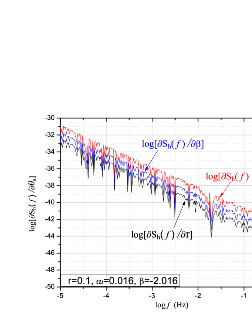
Figure 16: $\partial S_{h}/\partial\theta_{a}$ for $r=0.1,\beta=-2.016$ and $\alpha_{t}=0.016$

For $r=0.1$, $\alpha_{t}=0.016$ and $\beta=-2.016$ with SNR_C=179, we use the data streams generated in Section 8.2 and use (174) to numerically estimate $r$, and find that $r$ converges to $r_{ML}=0.1070$ after nine iterations.

As discussed before, in the neighborhood of $\bm{\bar{\theta}}$, one has the following Bayesian PDF in the parameter space

$$f(\bm{\theta})\propto\exp{[-\mathcal{L}]}\propto\exp\left[-\frac{1}{2}(\bm{\theta}-\bm{\bar{\theta}})\bm{F}(\bm{\theta}-\bm{\bar{\theta}})^{T}\right]\,.$$ (180)

The resolution of the parameters will be

$$\Delta\theta_{a}=1.96\sigma_{\theta_{a}}=1.96\sqrt{\left(\bm{F}^{-1}\right)_{aa}}\ \ {\rm\ at\ }95\%\,\,{\rm cl}\,,$$ (181)

and the correlation coefficient between two parameters will be

$$CR_{\theta_{a}\theta_{b}}\equiv\frac{\Big{\langle}\Big{(}\theta_{a}-\langle\theta_{a}\rangle\Big{)}\Big{(}\theta_{b}-\langle\theta_{b}\rangle\Big{)}\Big{\rangle}}{\sigma_{\theta_{a}}\sigma_{\theta_{a}}}=\frac{\left(\bm{F}^{-1}\right)_{ab}}{\sqrt{\left(\bm{F}^{-1}\right)_{aa}\left(\bm{F}^{-1}\right)_{bb}}}\,.$$ (182)

Note that $CR_{\theta_{a}\theta_{b}}=0$ indicates the independency of $\theta_{a}$ and $\theta_{b}$, and $|CR_{\theta_{a}\theta_{b}}|=1$ indicates the complete correlation of $\theta_{a}$ and $\theta_{b}$. Comparing Table 4 and Table 3, when $r$, $\alpha_{t}$ and $\beta$ are estimated at the same time, where Table 4 lists the resolutions, correlations and the corresponding values of SNR₁₂ ($\geq 3.29$), we find that when estimating the three parameters simultaneously, the resolution would get worse. This is due to the degeneracy of the three parameters as shown in Fig. 16, which can also be seen with $|CR_{\theta_{a}\theta_{b}}|\simeq 1$ in Table 4. Since the amplitude of the spectrum increases with $r$, $\beta$ and $\alpha_{t}$, when simultaneously estimating the three parameters, a larger estimated value of $\beta$ than its true value will lead to smaller estimated $r$ and $\alpha_{t}$ than their true values, or vice versa. This is reflected in the negative signs of $CR_{r\beta}$ and $CR_{\alpha_{t}\beta}$ in Table 4. Besides, we find that if estimating only two parameters with the third one fixed, the correlation coefficients between every two parameters are all negative, which is also an expected feature.

Table 4: Resolution of $r$, $\alpha_{t}$ and $\beta$ at $95\%$ cl for a pair, and correlations between them

$r$	$\alpha_{t}$	$\beta$	$\Delta r/r$	$\Delta\alpha_{t}$	$\Delta\beta$	$CR_{r\alpha_{t}}$	$CR_{r\beta}$	$CR_{\alpha_{t}\beta}$	SNRC
0.05	0.01	-2.016	$1.54\times 10^{4}$	$26.3$	$450$	$0.999697$	$-0.999923$	$-0.999925$	4.36
0.05	0.015	-2.016	$997$	$1.70$	$29.1$	$0.999724$	$-0.999930$	$-0.999932$	72.8
0.1	0	-1.93	$6.40\times 10^{3}$	$11.0$	$188$	$0.999634$	$-0.999907$	$-0.999910$	8.34
0.1	0.01	-2.016	$7.71\times 10^{3}$	$13.2$	$226$	$0.999696$	$-0.999923$	$-0.999925$	8.62
0.1	0.01	-1.93	$67.5$	$0.117$	$1.99$	$0.999460$	$-0.999863$	$-0.999867$	390
0.1	0.016	-2.016	$329$	$0.561$	$9.60$	$0.999681$	$-0.999919$	$-0.999921$	179

9 Conclusion

We have presented a study of statistical signal processing for the RGW detection by space-borne interferometers, using LISA as an example, and have shown how to estimate the RGW spectrum and parameters from the output signals in the future. We have given the relevant formulations of estimations, which apply to LISA, as well as to other space-borne interferometers with some appropriate modifications.

For a single interferometer, the Michelson is shown to have a better sensitivity than Sagnac, and symmetrized Sagnac, due to its greater transfer function $\mathcal{R}$, even though its noise is larger. A pair has the advantage of suppressing the noise level by cross-correlation, so that RGW signal in the cross-correlated output will be accumulating with observation time, leading to a higher sensitivity than a single case. We have given the expressions of SNR for both a single and a pair, which are $4\sim 6$ orders of magnitude higher than those of ground-based ones for the default RGW parameters. We have shown that a single is not practical to estimate the RGW spectrum when noise is dominantly large, because we do not know the precise noise that actually occurs in the data.

For a pair of interferometers, we have used the cross-correlated integrated signals $C$ in (5.2) and calculated SNR₁₂ as in (101) which provides a statistical criterion for detection of RGW. However, one cannot estimate the spectrum by the integrated signals $C$, because it is an integration over frequency. Assuming Gaussian output signals, and we have calculated the covariance of signals, obtained the Gaussian PDF, the likelihood function $\mathcal{L}$, and the Fisher matrix. By the Bayesian approach, we estimate one parameter and compute the resolution using $C$. In the second method, we have proposed applying the ensemble averaging method to estimate the spectrum, using the un-integrated output signals of a pair. (142) is the main formula. We have demonstrated by simulation that the method will be effective in estimating the spectrum. Besides, the method is simple and does not depend on detailed knowledge of the noise. For the third method, we have also studied the correlation variable of un-integrated signals from (148). We have obtained the formulations for estimation of the spectrum and parameters of RGW by the ML-estimation. Eqs. (169) and (174) are the main formulae. We have shown by simulations that the method is feasible when the data set is sufficiently large. This method uses the mean value for each segment and thus loses some fine information on the RGW spectrum, but it is capable of estimating all three parameters.

There are other effects to be analyzed that are not presented in this paper. In particular, other types of GWs that are different from RGW also exist in the Universe, and should be separated in order to estimate the RGW spectrum. GWs from a resolved astrophysical source, either periodic or short-lived, can be distinguished in principle. The real concern is the stochastic foreground that may by mixed with RGW. So far, the theoretical spectrum of this foreground is less known and highly model-dependent. For a definite model of the foreground spectrum, Ref. [44] discusses a discrimination method using the spectral shapes and the time modulation of the signal. The estimation of RGW in the presence of foreground will require substantial analysis and will be left for future work.

Acknowledgements

Y. Zhang is supported by NSFC Grant No. 11421303, 11675165, 11633001 SRFDP and CAS the Strategic Priority Research Program “The Emergence of Cosmological Structures” of the Chinese Academy of Sciences, Grant No. XDB09000000.

Appendix A The Fisher matrix for a pair

Given the data of cross-correlated signals $\bm{C}$ in (109) for a pair, we assume that the PDF is multivariate Gaussian

$$f({\bf C})=\frac{1}{(2\pi)^{\frac{N}{2}}\text{det}^{\frac{1}{2}}[\bm{\Sigma}]}\exp\left\{-\frac{1}{2}{(\bm{C}-\bm{\mu})}\ \bm{\Sigma}^{-1}\ \left(\bm{C}-\bm{\mu}\right)^{T}\right\}\,,$$ (A.1)

where the mean $\mu_{i}$ and covariance matrix $\Sigma_{ij}$ are given by (111) and (112) respectively, both being functions of the spectrum $S_{h}(f)$. The likelihood function is (dropping an irrelevant constant $\frac{1}{2}N\ln 2\pi$)

$$\mathcal{L}\equiv-\ln f=\frac{1}{2}\ln\text{det}[\bm{\Sigma}]+\frac{1}{2}{(\bm{C}-\bm{\mu})}\ \bm{\Sigma}^{-1}\ \left(\bm{C}-\bm{\mu}\right)^{T}.$$ (A.2)

The first order derivative is [74]

$$\frac{\delta\mathcal{L}}{\delta S_{h}(f)}= \frac{1}{2}\text{tr}\left(\bm{\Sigma}^{-1}\frac{\delta\bm{\Sigma}}{\delta S_{h}(f)}\right)-\frac{1}{2}{\bm{y}}\ \bm{\Sigma}^{-1}\frac{\delta\bm{\Sigma}}{\delta S_{h}(f)}\bm{\Sigma}^{-1}\ {\bm{y}}^{T}-\frac{\delta\bm{\mu}}{\delta S_{h}(f)}\bm{\Sigma}^{-1}\ {\bm{y}}^{T}$$ (A.3)

where $\bm{y}\equiv\bm{C}-\bm{\mu}$, and the second order derivative is

$$\frac{\delta^{2}\mathcal{L}}{\delta S_{h}(f)\delta S_{h}(f^{\prime})}= -\frac{1}{2}\text{tr}\left(\bm{\Sigma}^{-1}\frac{\delta\bm{\Sigma}}{\delta S_{h}(f^{\prime})}\bm{\Sigma}^{-1}\frac{\delta\bm{\Sigma}}{\delta S_{h}(f)}\right)+\frac{1}{2}\text{tr}\left(\bm{\Sigma}^{-1}\frac{\delta^{2}\bm{\Sigma}}{\delta S_{h}(f^{\prime})\delta S_{h}(f)}\right)$$

$$+{\bm{y}}\bm{\Sigma}^{-1}\frac{\delta\bm{\Sigma}}{\delta S_{h}(f^{\prime})}\bm{\Sigma}^{-1}\frac{\delta\bm{\Sigma}}{\delta S_{h}(f)}\bm{\Sigma}^{-1}\ {\bm{y}}^{T}+\frac{\delta\bm{\mu}}{\delta S_{h}(f^{\prime})}\ \bm{\Sigma}^{-1}\frac{\delta\bm{\Sigma}}{\delta S_{h}(f)}\bm{\Sigma}^{-1}\ {\bm{y}}^{T}$$

$$-\frac{1}{2}{\bm{y}}\ \bm{\Sigma}^{-1}\frac{\delta^{2}\bm{\Sigma}}{\delta S_{h}(f^{\prime})\delta S_{h}(f)}\bm{\Sigma}^{-1}\ {\bm{y}}^{T}-\frac{\delta^{2}\bm{\mu}}{\delta S_{h}(f^{\prime})\delta S_{h}(f)}\bm{\Sigma}^{-1}\ {\bm{y}}^{T}$$

$$+\frac{\delta\bm{\mu}}{\delta S_{h}(f)}\bm{\Sigma}^{-1}\frac{\delta\bm{\mu}^{T}}{\delta S_{h}(f^{\prime})}+\frac{\delta\bm{\mu}}{\delta S_{h}(f)}\bm{\Sigma}^{-1}\frac{\delta\bm{\Sigma}}{\delta S_{h}(f^{\prime})}\bm{\Sigma}^{-1}\ {\bm{y}}^{T}\,.$$ (A.4)

Taking the expectated value of the above yields the Fisher matrix

$$\mathcal{F}(f,f^{\prime})=\left\langle\frac{\delta^{2}\mathcal{L}}{\delta S_{h}(f)\delta S_{h}(f^{\prime})}\right\rangle= \frac{\delta\bm{\mu}}{\delta S_{h}(f)}\bm{\Sigma}^{-1}\frac{\delta\bm{\mu}^{T}}{\delta S_{h}(f^{\prime})}+\frac{1}{2}\text{tr}\left(\bm{\Sigma}^{-1}\frac{\delta\bm{\Sigma}}{\delta S_{h}(f^{\prime})}\bm{\Sigma}^{-1}\frac{\delta\bm{\Sigma}}{\delta S_{h}(f)}\right).$$ (A.5)

where $\left\langle{\bm{y}}^{T}\right\rangle=0$ and $\left\langle{\bm{y}}^{T}{\bm{y}}\right\rangle=\bm{\Sigma}$ are used. Using $\Sigma_{ij}$ of (112), one has

$$\frac{\delta\mathcal{L}}{\delta S_{h}(f)}= \sum^{N}_{l}\bigg{[}\frac{1}{2\mu_{l}}-\frac{C^{2}_{i}}{2b\mu_{i}^{2}}+\frac{1}{2b}\bigg{]}\frac{\delta\mu_{l}}{\delta S_{h}(f)},$$ (A.6)

$$\mathcal{F}(f,f^{\prime})= \sum_{l}^{N}\left(\frac{1}{b\mu_{l}}+\frac{1}{2\mu_{l}^{2}}\right)\frac{\delta\mu_{l}}{\delta S_{h}(f^{\prime})}\frac{\delta\mu_{l}}{\delta S_{h}(f)}\,,$$ (A.7)

where $b\equiv\frac{5}{3}$. By (111), the derivative of $\mu$ is given by

$$\frac{\delta\mu_{i}}{\delta S_{h}(f)}=\frac{T_{i}}{2b}\frac{\delta m}{\delta S_{h}(f)}=\frac{T_{i}}{2b}\frac{S_{h}(f)\,\gamma^{2}(f)}{M(f)}\left(1-\frac{N(f)}{M(f)}\right),~{}~{}~{}~{}~{}~{}~{}i=1,\cdots,N,$$ (A.8)

where $M(f)$ is defined by (95) and

$$N(f)\equiv\frac{1}{2}S_{h}(f)\frac{\partial{M(f)}}{\partial S_{h}(f)}=\frac{1}{2}\Big{[}S_{1n}(f)+S_{2n}(f)\Big{]}\mathcal{R}(f)S_{h}(f)+\left[\mathcal{R}^{2}(f)+\mathcal{R}_{12}^{2}(f)\right]S^{2}_{h}(f).$$ (A.9)

Using (111) and (A.8), the first order derivative is

$$\frac{\delta\mathcal{L}}{\delta S_{h}(f)}= \frac{1}{2}\frac{S_{h}(f)\,\gamma^{2}(f)}{M(f)}\left(1-\frac{N(f)}{M(f)}\right)\left(\frac{N}{m}-\frac{2}{m^{2}}\sum^{N}_{i}\frac{C^{2}_{i}}{T_{i}}+\frac{1}{2b^{2}}\sum^{N}_{i}T_{i}\right),$$ (A.10)

and the Fisher matrix is

$$\mathcal{F}(f,f^{\prime})= \left[\frac{S_{h}(f^{\prime})\,\gamma^{2}(f^{\prime})}{M(f^{\,{}^{\prime}})}\left(1-\frac{N(f^{\prime})}{M(f^{\prime})}\right)\right]\left[\frac{S_{h}(f)\,\gamma^{2}(f)}{M(f)}\left(1-\frac{N(f)}{M(f)}\right)\right]\frac{1}{2}\left(\frac{N}{m^{2}}+\frac{9}{25m}\sum_{l}^{N}T_{l}\right)\,.$$ (A.11)

From the above formulae, we also derive the Fisher matrix $F_{ab}$ for parameter estimation. Consider the PDF in (A.1)

$$f({\bf C};\bm{\theta})=\frac{1}{(2\pi)^{\frac{N}{2}}\text{det}^{\frac{1}{2}}[\bm{\Sigma}(\bm{\theta})]}\exp\left\{-\frac{1}{2}{\left(\bm{C}-\bm{\mu}(\bm{\theta})\right)}\ \bm{\Sigma}^{-1}(\bm{\theta})\ {\left(\bm{C}-\bm{\mu}(\bm{\theta})\right)}^{T}\right\}\,,$$ (A.12)

where $\mu(\theta)$ and $\bm{\Sigma}(\bm{\theta})$ now depend on the RGW parameters $\bm{\theta}=(r,\beta,\alpha_{t})$ through the theoretical spectrum $S_{h}(f)$ in (111) and (112). Using the result (A.6) (A.7), by the chain rule, one obtains the derivatives with respect to the parameters

$$\frac{\partial\mathcal{L}}{\partial\theta_{a}}=\frac{1}{2}\sum^{N}_{i}\bigg{[}\frac{1}{\mu_{i}}-\frac{C^{2}_{i}}{b\mu_{i}^{2}}+\frac{1}{b}\bigg{]}\frac{\partial\mu_{i}}{\partial\theta_{a}}\,,$$ (A.13)

$$\mathcal{F}_{ab}=\left\langle\frac{\partial^{2}\mathcal{L}}{\partial\theta_{a}\partial\theta_{b}}\right\rangle=\sum_{i}^{N}\left(\frac{1}{b\mu_{i}}+\frac{1}{2\mu_{i}^{2}}\right)\frac{\partial\mu_{i}}{\partial\theta_{a}}\frac{\partial\mu_{i}}{\partial\theta_{b}}\,.$$ (A.14)

Taking derivative of $\mu$ in Eq. (111) with respect to $\theta_{a}$ yields

$$\frac{\partial\mu_{i}}{\partial\theta_{a}}= \frac{T_{i}}{A}\int_{0}^{\infty}df\frac{S_{h}(f)\,\gamma^{2}(f)}{M(f)}\left(1-\frac{N(f)}{M(f)}\right)\,\frac{\partial S_{h}(f)}{\partial\theta_{a}},~{}~{}~{}~{}a=1,2,3,~{}~{}~{}i=1,\cdots,N.$$ (A.15)

Substituting (A.15) into (A.13) and (A.14) leads to (126) and (6.2).

References

- [1] A. Sesana, A. Vecchio and C. N. Colacino, Mon. Not. R. Astron. Soc. 390, 192-209 (2008); G. Janssen, G. Hobbs, M. McLaughlin, et al., arXiv:1501.00127 (2014).
- [2] B. P. Abbott, et al., Phys. Rev. Lett. 116, 061102 (2016); B. P. Abbott, et al., Phys. Rev. Lett. 116, 241103 (2016). B. P. Abbott, et al., Phys. Rev. Lett. 118, 221101 (2017).
- [3] B. P. Abbott, et al., Phys. Rev. Lett. 118, 121101 (2017) B. P. Abbott, et al., Phys. Rev. Lett. 116, 131102 (2016).
- [4] LIGO Scientific Collaboration and Virgo Collaboration , Nature 551, 85-88 (2017). B. P. Abbott, et al., Phys. Rev. Lett. 119, 161101 (2017).
- [5] B. P. Abbott, R. Abbott, T. D. Abbott, et al., Phys Rev Lett 120, 091101 (2018).
- [6] L. P. Grishchuk, Sov. Phys. JETP 40, 409 (1975). L. P. Grishchuk, Class. Quantum Grav. 14, 1445 (1997). L. P. Grishchuk, Lect. Notes Phys. 562, 167 (2001); arXiv:gr-qc/0002035. L. H. Ford and L. Parker, Phys. Rev. D 16, 1601 (1977). A. A. Starobinsky, JETP Lett. 30, 682(1979); Sov. Astron. Lett. 11, 133 (1985). R. Fabbri and M.D. Pollock, Phys. Lett. B125, 445 (1983). L.F. Abbott and M.B. Wise, Nucl. Phys. B224, 541 (1984). B. Allen, Phys. Rev. D 37, 2078 (1988). V. Sahni, Phys. Rev. D 42 453 (1990). M. Giovannini, Phys. Rev. D 60, 123511 (1999).
- [7] Y. Zhang, Y. Yuan, W. Zhao, and Y.T. Chen, Class. Quantum Grav. 22, 1383 (2005). Y. Zhang, X.Z. Er, T.Y. Xia, W. Zhao, and H.X. Miao, Class. Quantum Grav. 23, 3783 (2006) W. Zhao and Y. Zhang, Phys. Rev. D 74 043503 (2006).
- [8] D.G. Wang, Y. Zhang, and J.W. Chen, Phys. Rev. D 94, 044033 (2016)
- [9] M.L. Tong, Y. Zhang, et al., Class. Quantum Grav. 31 (2014) 035001
- [10] S. Weinberg, Phys. Rev. D 69, 023503 (2004).
- [11] H.X. Miao, Y. Zhang. Phys. Rev. D 75, 104009 (2007).
- [12] S. Wang, Y. Zhang, T.Y. Xia, and H.X. Miao, Phys. Rev. D 77, 104016 (2008).
- [13] K. N. Ananda, C. Clarkson and D. Wands, Phys.Rev.D 75, 123518 (2007). D. Baumann, P. Steinhardt, K. Takahashi and K. Ichiki, Phys. Rev. D 76, 084019 (2007).
- [14] B. Wang and Y. Zhang, Phys. Rev. D 96, 103522 (2017). Y. Zhang, F. Qin and B. Wang, Phys. Rev. D 96, 103523 (2017).
- [15] M.L. Tong and Y. Zhang, Phys. Rev. D 80, 084022 (2009).
- [16] G. F. Smoot et al., Astrophys. J. 396, L1 (1992). C. L. Bennett, et al, Astrophys. J. 396, L7 (1992).
- [17] C. L. Bennett et al., Astrophys. J. Suppl. 148, 1 (2003). E. Komatsu, et al, Astrophys. J. Suppl.192, 18 (2011)
- [18] G. Hinshaw, et al, Astrophys. J. Suppl.148 135, (2003)
- [19] Planck Collaboration, (Overview) A&A 594, A1 (2016).
- [20] Planck Collaboration, (Spectrum) A&A 594, A11 (2016) Planck Collaboration, (Parameter) A&A 594, A13 (2016) Planck Collaboration, (Inflation) A&A 594, A20 (2016).
- [21] G. Hobbs, PASA 22, 179 (2005); Class. Quantum Grav. 25, 114032 (2008). http://www.ipta4gw.org/; http://www.skatelescope.org/;
- [22] P. Bender et al., LISA Pre-Phase A Report (second edition) (1998) P. Bender, Class. Quantum Grav. 20, S301 (2003).
- [23] P. Amaro-Seoane et al., Class. Quantum Grav. 29, 124016 (2012),
- [24] P. Amaro-Seoane et al, arXiv:1702.00786 (2017).
- [25] K. Danzmann for the LISA study team, Class. Quantum Grav. 14, 1399 (1997). T. A. Prince et al, ”LISA: Probing the Universe with Gravitational Waves”, LISA Project internal report number LISA-LIST-RP-436 (2009). http://lisa.nasa.gov/ http://elisa-ngo.org/
- [26] F. B. Estabrook, M. Tinto, and J. W. Armstrong, Phys. Rev. D 62, 042002 (2000).
- [27] W. T. Ni, S. Shiomi, and A. C. Liao, Class. Quantum Grav. 21, S641 (2004); W. T. Ni, Int. J. Mod. Phys. D17, 921 (2008); Mod. Phys. Lett. A25, 922 (2010); Int.J.M.P.D, Vol. 22, No. 1, 1341004 (2013)
- [28] W. R. Hu and Y. L. Wu, National Science Review 5, 685-686 (2017); Z. G. Liu, Y. S. Piao, and C. F. Qiao, Modern Physics 5, 28-33 (2016); X. B. Wan, X. M. Zhang, and M. Li, Chinese Space Science and Technology 37, 110-116 (2017); Z. Wang, W. Sha, Z. Chen, et al., Chinese Optics 11,132-151 (2018).
- [29] A. Abramovici, et al. Science 256.5055, 325 (1992).
- [30] J. Abadie et al 2012 arXiv:1203.2674v2.
- [31] https://losc.ligo.org/archive/S6/ ; https://losc.ligo.org/timeline/ .
- [32] F. Acernese, et al, Class. Quantum Grav. 22, S869 (2005).
- [33] B. Willke, P. Aufmuth, C. Aulbert, et al. Class. Quantum Grav. 19, 1377 (2002).
- [34] Y. Aso, Y. Michimura, K. Somiya, et al. Phys. Rev. D 88, 043007 (2013).
- [35] R. Ballatini, et al., arXiv:gr-qc/0502054, INFN Technical Note INFN/TC-05/05, (2005).
- [36] A.M. Cruise and R.M.J. Ingley, Class. Quantum Grav.23, 6185 (2006); M.L. Tong and Y. Zhang, Chin. J. Astron. Astrophys. 8, 314 (2008).
- [37] F.Y. Li, M. X. Tang, D. P. Shi, Phys. Rev. D 67, 104008 (2003); M.L. Tong, Y. Zhang, and F. Y. Li, Phys.Rev. D 78, 024041 (2008).
- [38] M.M. Basko and A.G. Polnarev, Mon. Not. R. Astron. Soc., 191, 207 (1980); Sov. Astron. 24, 268 (1984); A.G. Polnarev, Sov. Astron. 29, 607 (1985); M. Zaldarriaga and D. D.Harari, Phys. Rev. D 52, 3276 (1995); A. Kosowsky, Annal. Phys.246, 49 (1996); M. Kamionkowski, A. Kosowsky, and A. Stebbins, Phys. Rev. D 55, 7368 (1997); W. Zhao and Y. Zhang, Phys. Rev. D 74, 083006 (2006); T.Y. Xia and Y. Zhang, Phys. Rev. D 78, 123005 (2008); Phys. Rev. D 79, 083002 (2009).
- [39] N. J. Cornish and S.L. Larson, Class. Quantum Grav. 20, S163 (2003); R. W. Hellings, Class. Quantum Grav. 20, 1019 (2003); N. J. Cornish and S. L. Larson, Phys. Rev. D 67, 103001 (2003); S. E. Timpano, L. J. Rubbo, N. J. Cornish, Phys. Rev. D 73, 122001 (2006); C. Ungarelli, A. Vecchio, Phys. Rev. D 64, 121501 (2001).
- [40] C. R. Evans, I. Iben Jr and L. Smarr, Astrophys. J. 323, 129 (1987); D. Hils, P. Bender and R. Webbink, Astrophys. J. 360, 75 (1990); P. L. Bender and D. Hils, Class. Quantum Grav. 14, 1439 (1997).
- [41] G. Nelemans, L. R. Yungelson, S. F. Portegies Zwart, et al., A&A 365, 491 (2001); G. Nelemans, S. F. Portegies Zwart, F. Verbunt, et al., A&A 368, 939 (2001). A. J. Ruiter, K. Belczynski, M. Benacquista, and K. Holley-Bockelmann, Astrophys. J. 693, 383 (2009);
- [42] N. Seto and A. Cooray, Phys.Rev. D 70, 123005 (2004);
- [43] M. R. Adams, N. J. Cornish and T. B. Littenberg, Phys. Rev. D 86, 124032 (2012).
- [44] M. R. Adams and N. J. Cornish, Phys. Rev. D 89, 022001 (2014).
- [45] A. Sesana, F. Haardt, P. Madau, et al., Astrophys. J. 611, 623 (2004); A. Sesana, F. Haardt, P. Madau, et al., Astrophys. J. 623, 23 (2005).
- [46] D. Hils and P. L. Bender, Astrophys. J. 537, 334 (2000); G. Nelemans, L. Yungelson and S. Portegies Zwart, Mon. Not. R. Astron. Soc. 349, 181 (2004). J.-E. Solheim, Publications of the Astronomical Society of the Pacific 122, 1133 (2010);
- [47] K. A. Arnaud, S. Babak, J. G. Baker, et al., Class. Quantum Grav. 24, S551 (2007); S. Babak, J. G. Baker, M. J. Benacquista, et al., Class. Quantum Grav. 25, 114037 (2008); Mock LISA Data Challenge Homepage astrogravs.nasa.gov/docs/mldc .
- [48] N. J. Cornish and J. Crowder, Phys. Rev. D 72, 043005 (2005).
- [49] N. J. Cornish and T. Robson, arXiv:1703.09858 (2017).
- [50] N. J. Cornish and T. B. Littenberg, Phys. Rev. D 76, 083006 (2007).
- [51] T. Robson and N. J. Cornish, Class. Quantum Grav. 34, 244002 (2017).
- [52] J. Crowder and N. J. Cornish, Phys. Rev. D 75, 043008 (2007).
- [53] C. W. Helstrom, Statistical theory of signal detection, New York : Pergamon Press, (1960). P. Jaranowski and A. Królak, Living Reviews in Relativity 8, 3 (2005).
- [54] L. S. Finn, Phys. Rev. D 46, 5236 (1992).
- [55] C. Cutler and E. E. Flanagan, Phys. Rev. D 49, 2658 (1994).
- [56] C. Cutler, Phys. Rev. D 57, 7089 (1998).
- [57] T. A. Moore and R. W. Hellings, Phys. Rev. D 65, 062001 (2002).
- [58] E. E. Flanagan, Phys. Rev. D 48, 2389 (1993).
- [59] B. Allen, in Proceedings of the Les Houches School of Physics, held in Les Houches, Haute Savoie, 26: 373 (1997), arXiv:gr-qc/9604033 ; B. Allen and J. D. Romano, Phys. Rev. D 59 (1999) 102001.
- [60] P. Binetruy, A. Bohe, C. Caprini, J. F. Dufaux, JCAP06, 027 (2012); C. Caprini, et al, JCAP04, 001 (2016).
- [61] C. Ungarelli and A. Vecchio, Phys. Rev. D 63, 064030 (2001).
- [62] de Vine, Glenn, et al., Phys. Rev. Lett. 104, 211103 (2010).
- [63] D.A. Shaddock, Phys.Rev. D 69, 022001 (2004).
- [64] M. Vallisneri, Phys.Rev. D 77, 042001 (2008).
- [65] N. J. Cornish & L. J. Rubbo, Phys.Rev. D 67, 022001 (2003).
- [66] N. J. Cornish and R. W. Hellings, Class. Quantum Grav. 20, 4851 (2003).
- [67] R. Schilling, Class. Quantum Grav. 14, 1513 (1997).
- [68] S. L. Larson, W. A. Hiscock and R. W. Hellings, Phys. Rev. D 62, 062001 (2000).
- [69] N. J. Cornish and S. L. Larson, Class. Quantum Grav. 18, 3473 (2001).
- [70] N. J. Cornish, Phys. Rev.D 65, 022004 (2001).
- [71] E. L. Robinson, J. D. Romano and A. Vecchio, Class. Quantum Grav. 25, 184019 (2008)
- [72] K. M. Gorski, et al, Astrophys. J. 430, L89 (1994). G. Jungman, M. Kamionkowski, A. Kosowsky, D.N. Spergel, Phys. Rev. D 54, 1332 (1996). M. Tegmark, A. N. Taylor, A. F. Heavens, Astrophys. J. 480, 22 (1997).
- [73] S. P. Oh, D. N. Spergel, and G. Hinshaw, Astrophys. J. 510, 551 (1999).
- [74] S. M. Kay, Fundamentals of statistical signal processing, Volume I: Estimation theory, Volume II: Detection theory, Pearson Education, (1993).
- [75] W.H.Press, S.A. Teukolsky, W.T.Vetterling, B.P. Flannery, Numerical Recipes: The Art of Scientific Computing, 2nd Ed., Cambridge University Press, (1992).
- [76] N. Seto, Phys. Rev. D 73, 063001 (2006).
- [77] L. Parker and D. J. Toms, Quantum Field Theory in Curved Spacetime: Quantized Fields and Gravity, Cambridge University Press, (2009). N. D. Birrell and P. C. W. Davies, Quantum Fields in Curved Space, Cambridge University Press, (1982).
- [78] M. Maggiore, Physics Reports 331, 283 (2000).
- [79] Y. Zhang, M.L. Tong, and Z.W. Fu, Phys. Rev. D 81, 101501(R) (2010).
- [80] D.Brill and J.Hartle, Phys. Rev.135, B271 (1964). D.Q. Su and Y. Zhang, Phys. Rev. D 85, 104012 (2012). S. Weinberg, Gravitation and Cosmology, John Wiley, (1972)
- [81] A. Kosowsky and M. S. Turner, Phys. Rev. D 52, R1739 (1995).
- [82] M. Vallisneri, J. Crowder, and M. Tinto, Class. Quantum Grav. 25, 065005 (2008).
- [83] L. J. Rubbo, N. J. Cornish and O. Poujade, Phys. Rev. D 69, 082003 (2004).
- [84] M. Tinto and J.W. Armstrong, Phys. Rev. D 59, 102003 (1999) M. Tinto, F. B. Estabrook and J. Armstrong, Phys. Rev. D 69, 082001 (2004). M. Tinto, M. Vallisneri and J. W. Armstrong, Phys. Rev. D 71, 041101 (2005).
- [85] J. W. Armstrong, F. B. Estabrook, and M. Tinto, Astrophys. J. 527, 814 (1999). T. A. Prince, M. Tinto, S. L. Larson, and J. W. Armstrong, Phys. Rev. D 66, 122002 (2002).
- [86] H. Kudoh and A. Taruya, Phys. Rev. D 71, 024025, (2005).
- [87] K. S. Thorne, in 300 Years of Gravitation, edited by S. W. Hawking and W. Israel, Cambridge University Press, Cambridge, (1987)
- [88] M. Tinto, J. W. Armstrong and F. B. Estabrook, Phys. Rev. D 63, 021101 (2000).
- [89] LIGO Collaboration and VIRGO Collaboration, Nature 460, 990 (2009).
- [90] J. R. Gair, M. Vallisneri, S.L. Larson, J.G. Baker, Living Reviews in Relativity 16, 7 (2013).