Theoretical results for charged-Higgs production

Nikolaos Kidonakis

Department of Physics
Kennesaw State University, Kennesaw, GA 30144, USA

I discuss charged-Higgs production via two different processes: in association with a top quark, and in association with a $W$ boson. I present total cross sections and differential distributions that include higher-order corrections from soft and collinear gluon emission through aN³LO. I show that these radiative corrections are significant.

PRESENTED AT

CIPANP2018
Palm Springs, California, May 29–June 3, 2018

1 Introduction

Since the discovery of the (neutral) Higgs boson a lot of attention has been given to its properties and the determination whether it is the Standard Model Higgs. However, any discovery of a charged Higgs boson would be evidence of new physics, and the LHC can observe or exclude such a possibility in a wide mass range.

Here I present results for two distinct production processes of charged Higgs bosons in the MSSM (or other 2-Higgs doublet models). I will discuss the processes $bg\rightarrow tH^{-}$ and $b{\overline{b}}\rightarrow H^{-}W^{+}$.

Higher-order QCD corrections are significant for both processes. Furthermore, since the processes involve very massive final states, soft-gluon corrections are important and constitute the bulk of the corrections. Below I present theoretical results for these corrections, and numerical results for cross sections and distributions at LHC energies.

2 $tH^{-}$ production

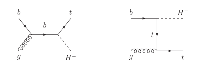
Figure 1: Lowest-order diagrams for $bg\rightarrow tH^{-}$.

The leading-order cross section for $bg\rightarrow tH^{-}$ is proportional to $\alpha\alpha_{s}(m_{b}^{2}\tan^{2}\beta+m_{t}^{2}\cot^{2}\beta)$, where $\tan\beta=v_{2}/v_{1}$ is the ratio of the vacuum expectation values of the two Higgs doublets. The lowest-order diagrams are shown in Fig. 1.

Fixed-order QCD and SUSY-QCD corrections through NLO have been calculated for this process in Refs. [1, 2, 3, 4, 5, 6, 7, 8, 9]. Soft-gluon terms constitute a numerically dominant piece of the QCD corrections.

With the momenta assignments, $b(p_{b})+g(p_{g})\longrightarrow t(p_{t})+H^{-}(p_{H})$, we define the usual variables $s=(p_{b}+p_{g})^{2}$, $t=(p_{b}-p_{t})^{2}$, $u=(p_{g}-p_{t})^{2}$, and furthermore the threshold variable $s_{4}=s+t+u-m_{t}^{2}-m_{H}^{2}$ which goes to 0 at partonic threshold. Soft-gluon corrections appear in the cross section as logarithms of the form $[\ln^{k}(s_{4}/m_{H}^{2})/s_{4}]_{+}$ [10, 11, 12].

We resum these soft corrections for the double-differential cross section at NNLL accuracy, using two-loop soft anomalous dimensions [11, 12, 13]. Taking moments of the partonic cross section, ${\hat{\sigma}}(N)=\int(ds_{4}/s)\;e^{-Ns_{4}/s}{\hat{\sigma}}(s_{4})$, we write the factorized expression for the dimensionally regularized cross section

$${\hat{\sigma}}^{bg\rightarrow tH^{-}}(N,\epsilon)=\left(\prod_{i=b,g}J_{i}\left(N,\mu,\epsilon\right)\right)H^{bg\rightarrow tH^{-}}\left(\alpha_{s}(\mu)\right)\;S^{bg\rightarrow tH^{-}}\left(\frac{m_{H}}{N\mu},\alpha_{s}(\mu)\right)$$ (1)

where $J_{i}$ denote functions for the incoming $b$-quark and gluon, $H^{bg\rightarrow tH^{-}}$ is the hard function, and $S^{bg\rightarrow tH^{-}}$ is the soft function.

The soft anomalous dimension $\Gamma_{S}^{bg\rightarrow tH^{-}}$ controls the evolution of $S^{bg\rightarrow tH^{-}}$, resulting in the exponentiation of logarithms of $N$. Writing the perturbative series for $\Gamma_{S}^{bg\rightarrow tH^{-}}$ as

$$\Gamma_{S}^{bg\rightarrow tH^{-}}=\frac{\alpha_{s}}{\pi}\Gamma_{S}^{(1)}+\left(\frac{\alpha_{s}}{\pi}\right)^{2}\Gamma_{S}^{(2)}+\cdots\,,$$ (2)

a one-loop calculation gives [10]

$$\Gamma_{S}^{(1)}=C_{F}\left[\ln\left(\frac{m_{t}^{2}-t}{m_{t}\sqrt{s}}\right)-\frac{1}{2}\right]+\frac{C_{A}}{2}\ln\left(\frac{m_{t}^{2}-u}{m_{t}^{2}-t}\right)$$ (3)

while a two-loop calculation gives [11]

$$\Gamma_{S}^{(2)}=\left[C_{A}\left(\frac{67}{36}-\frac{\zeta_{2}}{2}\right)-\frac{5}{18}n_{f}\right]\Gamma_{S}^{(1)}+C_{F}C_{A}\frac{(1-\zeta_{3})}{4}\,.$$ (4)

We then expand the resummed cross section and invert to momentum space, thus deriving approximate cross sections at NNLO and N³LO. The approximate NNLO (aNNLO) soft-gluon corrections are

$$\frac{d^{2}{\hat{\sigma}}_{\rm aNNLO}^{(2)\,bg\rightarrow tH^{-}}}{dt\,du}=F_{\rm LO}^{bg\rightarrow tH^{-}}\frac{\alpha_{s}^{2}}{\pi^{2}}\sum_{k=0}^{3}C_{k}^{(2)}\left[\frac{\ln^{k}(s_{4}/m_{H}^{2})}{s_{4}}\right]_{+}$$ (5)

with coefficients $C_{3}^{(2)}=2(C_{F}+C_{A})^{2}$ and

$$C_{2}^{(2)} = (C_{F}+C_{A})\left\{3C_{F}\left[2\ln\left(\frac{m_{t}^{2}-t}{m_{t}\sqrt{s}}\right)-2\ln\left(\frac{m_{H}^{2}-u}{m_{H}^{2}}\right)-1\right]\right.$$ (6)

$$\left.{}-3C_{A}\left[\ln\left(\frac{m_{t}^{2}-t}{m_{t}^{2}-u}\right)+2\ln\left(\frac{m_{H}^{2}-t}{m_{H}^{2}}\right)\right]-3(C_{F}+C_{A})\ln\left(\frac{\mu_{F}^{2}}{s}\right)-\frac{\beta_{0}}{2}\right\}\,.$$

The expressions for $C_{1}^{(2)}$ and $C_{0}^{(2)}$ are much longer [11].

The approximate N³LO (aN³LO) soft-gluon corrections are:

$$\frac{d^{2}{\hat{\sigma}}_{\rm aN^{3}LO}^{(3)\,bg\rightarrow tH^{-}}}{dt\,du}=F_{\rm LO}^{bg\rightarrow tH^{-}}\frac{\alpha_{s}^{3}}{\pi^{3}}\sum_{k=0}^{5}C_{k}^{(3)}\left[\frac{\ln^{k}(s_{4}/m_{H}^{2})}{s_{4}}\right]_{+}$$ (7)

with coefficients $C_{3}^{(3)}=\frac{1}{2}(C_{F}+C_{A})^{3}$, etc.

We now present numerical results for $tH^{-}$ production at LHC energies. We use MMHT2014 NNLO pdf [14] in our calculations.

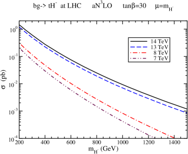
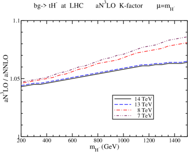
Figure 2: Total aN³LO cross sections (left) and aN³LO /aNNLO ratios (right) for $tH^{-}$ production.

The aN³LO cross sections at LHC energies are plotted in Fig. 2. The left plot gives the total cross sections at each LHC energy as functions of charged Higgs mass while the plot on the right shows the aN³LO/aNNLO ratios.

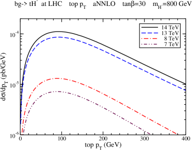
Figure 3: Top-quark $p_{T}$ distributions at aNNLO in $tH^{-}$ production for a charged Higgs mass of (left) 300 GeV and (right) 800 GeV.

The top-quark aNNLO transverse-momentum, $p_{T}$, distributions at LHC energies are plotted in Fig. 3. The left plot is for a charged Higgs mass of 300 GeV, while the right plot uses 800 GeV.

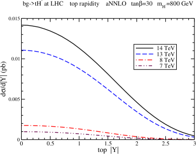
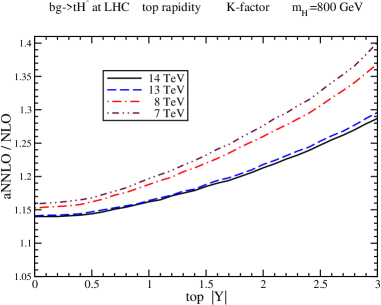
Figure 4: Top-quark rapidity distributions at aNNLO (left) and aNNLO/NLO ratios (right) in $tH^{-}$ production for a charged Higgs mass of 800 GeV.

The top-quark aNNLO rapidity distributions at LHC energies are plotted in Fig. 4 for a charged Higgs mass of 800 GeV. As the aNNLO/NLO ratios in the plot on the right show, the higher-order soft-gluon corrections are large, and increase sharply for larger values of rapidity.

The fact that soft-gluon corrections are large and dominate the corrections for $tH^{-}$ production is also consistent with analogous results for $t{\overline{t}}$ production [15, 16] and single-top [11, 16, 17] production.

3 $H^{-}W^{+}$ production

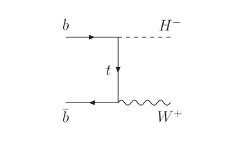
Figure 5: Lowest-order diagram for $b{\overline{b}}\rightarrow H^{-}W^{+}$.

We continue with $H^{-}W^{+}$ production via the process

$$b(p_{1})\,+\,{\overline{b}}\,(p_{2})\rightarrow H^{-}(p_{3})\,+W^{+}(p_{4})\,,$$ (8)

for which the lowest-order diagram is shown in Fig. 5.

Fixed-order radiative corrections were calculated for this process in Refs. [18, 19, 20, 21, 22, 23, 24, 25, 26, 27, 28, 29, 30, 31, 32, 33, 34, 35]. Soft-gluon contributions are a numerically large and dominant part of higher-order corrections.

Again, defining $s=(p_{1}+p_{2})^{2}$, $t=(p_{1}-p_{3})^{2}$, $u=(p_{2}-p_{3})^{2}$ and $s_{4}=s+t+u-m_{H}^{2}-m_{W}^{2}$, the soft-gluon corrections appear as terms of the form $[\ln^{k}(s_{4}/m_{H}^{2})/s_{4}]_{+}$ [36]. In addition, we include collinear terms of the form $(1/m_{H}^{2})\ln^{k}(s_{4}/m_{H}^{2})$ since they are numerically important, as was also found for the related process $b{\overline{b}}\rightarrow H$ in Ref. [37].

We write again a factorized expression for the cross section as

$${\hat{\sigma}}^{b{\overline{b}}\rightarrow H^{-}W^{+}}(N,\epsilon)=\left(\prod_{i=b,{\overline{b}}}J_{i}\left(N,\mu,\epsilon\right)\right)H^{b{\overline{b}}\rightarrow H^{-}W^{+}}\left(\alpha_{s}(\mu)\right)\;S^{b{\overline{b}}\rightarrow H^{-}W^{+}}\left(\frac{m_{H}}{N\mu},\alpha_{s}(\mu)\right)\,,$$ (9)

where $J_{i}$ denote functions for the incoming $b$ and ${\overline{b}}$ quarks, $H^{b{\overline{b}}\rightarrow H^{-}W^{+}}$ is the hard function, and $S^{b{\overline{b}}\rightarrow H^{-}W^{+}}$ is the soft function. We perform the resummation of collinear and soft-gluon corrections, and expand to fixed order.

The aNNLO collinear and soft-gluon corrections are [36]

$$\frac{d^{2}{\hat{\sigma}}_{\rm aNNLO}^{(2)\,b{\overline{b}}\rightarrow H^{-}W^{+}}}{dt\,du}=F_{LO}^{b{\overline{b}}\rightarrow H^{-}W^{+}}\frac{\alpha_{s}^{2}}{\pi^{2}}\left\{-C_{3}^{(2)}\frac{1}{m_{H}^{2}}\ln^{3}\left(\frac{s_{4}}{m_{H}^{2}}\right)+\sum_{k=0}^{3}C_{k}^{(2)}\left[\frac{\ln^{k}(s_{4}/m_{H}^{2})}{s_{4}}\right]_{+}\right\}$$ (10)

with $C_{3}^{(2)}=8C_{F}^{2}$

$$C_{2}^{(2)}=-12C_{F}^{2}\left(\ln\left(\frac{(t-m_{W}^{2})(u-m_{W}^{2})}{m_{H}^{4}}\right)+\ln\left(\frac{\mu_{F}^{2}}{s}\right)\right)-\frac{11}{3}C_{F}C_{A}+\frac{2}{3}C_{F}n_{f}\,.$$ (11)

The expressions for $C_{1}^{(2)}$ and $C_{0}^{(2)}$ are much longer and are given in [36].

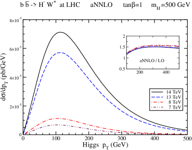
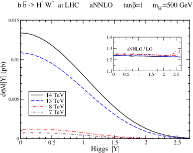
Figure 6: The charged-Higgs aNNLO $p_{T}$ (left) and rapidity (right) distributions in $H^{-}W^{+}$ production.

Next, we present results for $H^{-}W^{+}$ production at LHC energies. We use the MMHT2014 NNLO pdf [14] in our calculations but note that results using CT14 pdf [38] are nearly the same.

In Fig. 6 we present the charged-Higgs $p_{T}$ and rapidity distributions at aNNLO. The inset plots show the aNNLO/LO ratios, which show that the soft-gluon corrections are very significant. These results are also in line with analogous results for $W$ production that were presented in [39].

The aN³LO collinear and soft-gluon corrections are

$$\frac{d^{2}{\hat{\sigma}}_{\rm aN^{3}LO}^{(3)\,b{\overline{b}}\rightarrow H^{-}W^{+}}}{dt\,du}=F_{LO}^{b{\overline{b}}\rightarrow H^{-}W^{+}}\frac{\alpha_{s}^{3}}{\pi^{3}}\left\{-C_{5}^{(3)}\frac{1}{m_{H}^{2}}\ln^{5}\left(\frac{s_{4}}{m_{H}^{2}}\right)+\sum_{k=0}^{5}C_{k}^{(3)}\left[\frac{\ln^{k}(s_{4}/m_{H}^{2})}{s_{4}}\right]_{+}\right\}$$ (12)

with $C_{5}^{(3)}=8C_{F}^{3}$, etc. [36].

The aN³LO corrections are numerically small but they have big uncertainties. Therefore we do not show numerical results for them here.

4 Summary

I have presented new results through aN³LO for charged Higgs production in association with a top quark or a $W$ boson. Soft-gluon corrections have been derived from NNLL resummation at aNNLO and aN³LO.

Total cross sections for $tH^{-}$ production have been presented at aN³LO and it is shown that the soft-gluon corrrections are large. Top-quark $p_{T}$ and rapidity distributions in $tH^{-}$ production were also presented at aNNLO.

I have also presented cross sections and charged-Higgs $p_{T}$ and rapidity distributions in $H^{-}W^{+}$ production at aNNLO. The higher-order soft-gluon corrections are very significant at LHC energies.

References

- [1] A. Belyaev, D. Garcia, J. Guasch, and J. Sola, Phys. Rev. D 65, 031701 (2002) [hep-ph/0105053]; JHEP 0206, 059 (2002) [hep-ph/0203031].
- [2] S.-H. Zhu, Phys. Rev. D 67, 075006 (2003) [hep-ph/0112109].
- [3] G.-P. Gao, G.-R. Lu, Z.-H. Xiong, and J.M. Yang, Phys. Rev. D 66, 015007 (2002) [hep-ph/0202016].
- [4] T. Plehn, Phys. Rev. D 67, 014018 (2003) [hep-ph/0206121].
- [5] E.L. Berger, T. Han, J. Jiang, and T. Plehn, Phys. Rev. D 71, 115012 (2005) [hep-ph/0312286].
- [6] P. Wu, W.-G. Ma, R.-Y. Zhang, Y. Jiang, L. Han, and L. Guo, Phys. Rev. D 73, 015012 (2006) [hep-ph/0601069]; (E) 80, 059901 (2009).
- [7] S. Dittmaier, M. Kramer, M. Spira, and M. Walser, Phys. Rev. D 83, 055005 (2011) [arXiv:0906.2648 [hep-ph]].
- [8] M. Flechl, R. Klees, M. Kramer, M. Spira, and M. Ubiali, Phys. Rev. D 91, 075015 (2015) [arXiv:1409.5615 [hep-ph]].
- [9] C. Degrande, M. Ubiali, M. Wiesemann, and M. Zaro, JHEP 1510, 145 (2015) [arXiv:1507.02549 [hep-ph]].
- [10] N. Kidonakis, Int. J. Mod. Phys. A 19, 1793 (2004) [hep-ph/0303186]; Mod. Phys. Lett. A 19, 405 (2004) [hep-ph/0401147]; JHEP 0505, 011 (2005) [hep-ph/0412422]; Phys. Rev. D 73, 034001 (2006) [hep-ph/0509079].
- [11] N. Kidonakis, Phys. Rev. D 82, 054018 (2010) [arXiv:1005.4451 [hep-ph]].
- [12] N. Kidonakis, Phys. Rev. D 94, 014010 (2016) [arXiv:1605.00622 [hep-ph]].
- [13] N. Kidonakis, Phys. Rev. Lett. 102, 232003 (2009) [arXiv:0903.2561 [hep-ph]]; Int. J. Mod. Phys. A 31, 1650076 (2016) [arXiv:1601.01666 [hep-ph]].
- [14] L.A. Harland-Lang, A.D. Martin, P. Molytinski and R.S. Thorne, Eur. Phys. J. C 75, 204 (2015) [arXiv:1412.3989 [hep-ph]].
- [15] N. Kidonakis, Phys. Rev. D 90, 014006 (2014) [arXiv:1405.7046 [hep-ph]]; 91, 031501(R) (2015) [arXiv:1411.2633 [hep-ph]]; 91, 071502(R) (2015) [arXiv:1501.01581 [hep-ph]].
- [16] N. Kidonakis, in Physics of Heavy Quarks and Hadrons, HQ2013 [arXiv:1311.0283 [hep-ph]]; Int. J. Mod. Phys. A (in press) [arXiv:1806.03336 [hep-ph]].
- [17] N. Kidonakis, Phys. Rev. D 81, 054028 (2010) [arXiv:1001.5034 [hep-ph]]; 83, 091503(R) (2011) [arXiv:1103.2792 [hep-ph]]; 88, 031504(R) (2013) [arXiv:1306.3592 [hep-ph]]; 93, 054022 (2016) [arXiv:1510.06361 [hep-ph]]; 96, 034014 (2017) [arXiv:1612.06426 [hep-ph]].
- [18] D.A. Dicus, J.L. Hewett, C. Kao, and T.G. Rizzo, Phys. Rev. D 40, 787 (1989).
- [19] D.A. Dicus and C. Kao, Phys. Rev. D 41, 832 (1990).
- [20] Y.S. Yang, C.S. Li, L.G. Jin, and S.H. Zhu, Phys. Rev. D 62, 095012 (2000) [hep-ph/0004248].
- [21] F. Zhou, W.-G. Ma, Y. Jiang, L. Han, and L.-H. Wan, Phys. Rev. D 63, 015002 (2001).
- [22] O. Brein, W. Hollik, and S. Kanemura, Phys. Rev. D 63, 095001 (2001) [hep-ph/0008308].
- [23] W. Hollik and S.-H. Zhu, Phys. Rev. D 65, 075015 (2002) [hep-ph/0109103].
- [24] E. Asakawa, O. Brein, and S. Kanemura, Phys. Rev. D 72, 055017 (2005) [hep-ph/0506249].
- [25] J. Zhao, C.S. Li, and Q. Li, Phys. Rev. D 72, 114008 (2005) [hep-ph/0509369].
- [26] D. Eriksson, S. Hesselbach, and J. Rathsman, Eur. Phys. J. C 53, 267 (2008) [hep-ph/0612198]; J. Phys. Conf. Ser. 110, 072008 (2008) [arXiv:0710.0526].
- [27] J. Gao, C.S. Li, and Z. Li, Phys. Rev. D 77, 014032 (2008) [arXiv:0710.0826 [hep-ph]].
- [28] M. Hashemi, Phys. Rev. D 83, 055004 (2011) [arXiv:1008.3785 [hep-ph]].
- [29] S.-S. Bao, Y. Tang, and Y.-L. Wu, Phys. Rev. D 83, 075006 (2011) [arXiv:1011.1409 [hep-ph]].
- [30] T.N. Dao, W. Hollik, and D.N. Le, Phys. Rev. D 83, 075003 (2011) [arXiv:1011.4820 [hep-ph]].
- [31] M. Aoki, R. Guedes, S. Kanemura, S. Moretti, R. Santos, and K. Yagyu, Phys. Rev. D 84, 055028 (2011) [arXiv:1104.3178 [hep-ph]].
- [32] A. Alves, E.Ramirez Barreto, and A.G. Dias, Phys. Rev. D 84, 075013 (2011) [arXiv:1105.4849 [hep-ph]].
- [33] S.-S. Bao, X. Gong, H.-L. Li, S.-Y. Li, and Z.-G. Si, Phys. Rev. D 85, 075005 (2012) [arXiv:1112.0086 [hep-ph]].
- [34] R. Enberg, R. Pasechnik, and O. Stal, Phys. Rev. D 85, 075016 (2012) [arXiv:1112.4699 [hep-ph]].
- [35] G.-L. Liu, F. Wang, and S. Yang, Phys. Rev. D 88, 115006 (2013) [arXiv:1302.1840 [hep-ph]].
- [36] N. Kidonakis, Phys. Rev. D 97, 034002 (2018) [arXiv:1704.08549 [hep-ph]]; in Proceedings of DPF 2017, eConf C170731 [arXiv:1709.06976 [hep-ph]].
- [37] N. Kidonakis, Phys. Rev. D 77, 053008 (2008) [arXiv:0711.0142 [hep-ph]].
- [38] S. Dulat, T.-J. Hou, J. Gao, M. Guzzi, J. Huston, P. Nadolsky, J. Pumplin, C. Schmidt, D. Stump and C.-P. Yuan, Phys. Rev. D 93, 033006 (2016) [arXiv:1506.07443 [hep-ph]].
- [39] N. Kidonakis and A. Sabio Vera, JHEP 0402, 027 (2004) [hep-ph/0311266]; N. Kidonakis and R.J. Gonsalves, Phys. Rev. D 89, 094022 (2014) [arXiv:1404.4302 [hep-ph]].