Planar and Radial Kinks in Nonlinear Klein-Gordon Models:
Existence, Stability and Dynamics

Abstract

We consider effectively one-dimensional planar and radial kinks in two-dimensional nonlinear Klein-Gordon models and focus on the sine-Gordon model and the $\phi^{4}$ variants thereof. We adapt an adiabatic invariant formulation recently developed for nonlinear Schrödinger equations, and we study the transverse stability of these kinks. This enables us to characterize one-dimensional planar kinks as solitonic filaments, whose stationary states and corresponding spectral stability can be characterized not only in the homogeneous case, but also in the presence of external potentials. Beyond that, the full nonlinear (transverse) dynamics of such filaments are described using the reduced, one-dimensional, adiabatic invariant formulation. For radial kinks, this approach confirms their azimuthal stability. It also predicts the possibility of creating stationary and stable ring-like kinks. In all cases we corroborate the results of our methodology with full numerics on the original sine-Gordon and $\phi^{4}$ models.

I Introduction

The study of the existence, transverse stability, and dynamics of coherent structures that have an effective dimensionality lower than that of the space in which they live, is one that has a time-honored history in areas such as nonlinear optics agrawal and atomic physics, especially in connection with Bose-Einstein condensates (BECs) stringari ; siambook . This is, among other reasons, due to the remarkable observation and associated analysis of the potential of coherent structures to undergo transverse instability kuzne ; kidep which leads to the spontaneous formation of structures that are particular to (and more robust within) the higher-dimensional setting, such as vortices in two-dimensional (2D) settings pismen , and vortex lines and rings in 3D settings siambook . It is worthwhile to note that this type of instability, e.g., for prototypical structures such as the so-called dark solitons (which are ubiquitous in both nonlinear optics Kivshar-LutherDavies and atomic BECs djf ) has been explored extensively at the experimental level too. In particular, the production of vortices in the former setting tikh and vortex rings in the latter watching through this mechanism has been verified. This, in turn, has made this a subject of persisting theoretical interest aimed both towards analyzing and understanding such instabilities smirnov ; hoefer ; wang1 ; wang2 , as well as towards avoiding them us .

As a related topic, it should be mentioned that higher dimensional settings also enable the consideration of different geometric configurations, e.g. ones with different curvature etc. In particular, with regard to the kinklike dark soliton structures, naturally an extension of such a 1D heteroclinic structure to 2D may involve a planar front (like a 1D wall separating left from right or top from bottom). However, it is also possible to form such structures in a ring-like shape. The latter pattern, the so-called ring dark soliton has again been explored both in optics kivyang ; rings ; rings1 and in BECs rings2 ; rings3 ; rings4 . Extensions to even higher dimensions such as shells of either planar or spherical form have also been explored in 3D; see, e.g., kivyang ; carr ; wenlong ; hau among many others.

The focus of the present work is to generalize some of the ideas that have recently proved useful in analyzing such structures in atomic BECs wang1 ; wang2 to another setting with a time-honored history, namely Klein-Gordon (KG) equations. Some prototypical examples among these field theories consist of the sine-Gordon (sG) equation, to which whole volumes have been dedicated sgbook , as well as the $\phi^{4}$ model. The latter is among the principal models for phase transitions in statistical physics parisi , a toy model widely used in ferroelectrics, polymeric chains, and nuclear physics among many others schonfeld , but also a classical (as well as quantum) field theory of particular interest in its own right belova . In these KG settings, which have been extensively explored over the years (see e.g. Ref. kivsharmalomed for a review), the study of excitations such as, e.g., radial kinks has been a topic of particular interest from early on. One can note numerous attempts to explore the kink dynamics in two- and even in three-dimensions christiansen ; geicke ; bogolub , as well as to develop equations of motion, e.g., for moving radial kinks samuelsen , or to appreciate the rate of radiation of shrinking radial kinks malo . Efforts along similar lines both theoretically and numerically have been pursued for the $\phi^{4}$ model maloma ; gleiser . A recent summary of the relevant earlier activity, and suggestion to utilize radial kinks as sources of a fast breather (emerging from their detrimental collision with boundaries) can be found in Ref. caputo .

Our aim in the present work is to adapt some of the earlier ideas presented in the context of transverse instabilities in the nonlinear Schrödinger (NLS) settings in Ref. wang1 ; wang2 to the realm of the KG prototypical models (sG and $\phi^{4}$). In previous works, various authors have described the evolution of radial kinks due to curvature effects christiansen ; geicke ; bogolub ; samuelsen . However, these works only focused on the case of purely radial dynamics where the kink remains perfectly circular and does not undergo any transverse perturbation —with the notable exception of Ref. Boris , which described the dynamics of elliptical solutions (pulsons) in the sG model. In contrast, in the present work, formulating a Hamiltonian framework for KG models and adapting the solitonic filament method will allow us to examine the existence and stability of longitudinal kinks in two dimensions and, importantly, to formulate reduced PDEs for their transverse evolution. Furthermore, this methodology will also enable us to understand what role external (nonlinear) potentials can play in either stabilizing or destabilizing such kinks. Such potentials are certainly possible in practical applications. For instance, in Chap. 1 of Ref. sgbook , the presence of potential terms in the form considered herein has been connected to the presence of spatial inhomogeneities in the context of Josephson junctions; see also Ref. mal27 . Another example of this type is the so-called Josephson window junction, leading to the “dressing” (width variation) of the kinklike fluxon jgc2 . We will argue that not only are such potentials interesting in their own right, but rather they will also serve to create an unprecedented example of a stable radially symmetric kinklike structure in both prototypical KG models. As an aside, we will unveil how the transverse instabilities that are quite detrimental for kinklike (dark soliton) structures in optics/BEC are absent in the KG settings considered. Instead, the transverse undulations will be seen to be of a benign oscillatory character. Overall, we believe that this perspective will shed light on the (as we will call it) filamentary dynamics of kinks in higher dimensional KG models, and it will open new directions for their stabilization and practical use in applications, such as Josephson junction arrays sgbook .

Our presentation is structured as follows. In the next section, we detail the theoretical analysis of the transverse dynamics of quasi-1D structures. We start by recalling the instructive example of NLS from earlier works wang1 ; wang2 to which we later compare our KG case examples. We present the theory for KG structures by first focusing on the case of “standard” rectilinear 1D kinks embedded within a 2D domain. Then, we present the more involved case of radial kinks. In Sec. III we showcase the theoretical results presented in Sec. II by comparing the stability predictions and dynamics of our approach against the corresponding ones for the original KG models. Finally, in the last section, we conclude by presenting a number of challenges for future work in this theme.

II Theoretical Analysis

II.1 A Preamble: the NLS Case

We start our theoretical analysis by briefly revisiting the planar NLS dark soliton in the 2D setting. The model, in that case relevant to atomic Bose-Einstein condensates as well as nonlinear optics stringari ; siambook ; agrawal , is the defocusing nonlinear Schrödinger of the form:

$$iu_{t}=-\frac{1}{2}u_{xx}+|u|^{2}u+V(x)u.$$ (1)

When the potential is absent (i.e., $V(x)=0$), the energy of the model is conserved and it has the functional form:

$$H_{\rm 1D}=\frac{1}{2}\int_{-\infty}^{\infty}\left[|u_{x}|^{2}+\left(|u|^{2}-\mu\right)^{2}\right]dx,$$ (2)

where the constant $\mu$ represents the chemical potential. In this same $V(x)=0$ case, the prototypical exact solitary waves of the model are of the form Kivshar-LutherDavies ; djf :

$$u(x,t)=e^{-i\mu t}\left[\beta\tanh\left(\beta(x-{\xi})\right)+iv\right],$$ (3)

where $\beta=\sqrt{\mu-v^{2}}$ and the speed of the kink is $\dot{\xi}=v$. The energy of such a configuration is [substituting Eq. (3) in Eq. (2)] $H_{\rm 1D}=(4/3)(\mu-\dot{\xi}^{2})^{3/2}$. The fundamental idea of Ref. konotop_pit was to use this energy as an adiabatic invariant (AI) even in the case in which there is a potential with the modification that locally the chemical potential $\mu$ becomes $\mu-V(x)$ in the presence of such a term. From this AI quantity:

$$H_{\rm 1D}=\frac{4}{3}\left(\mu-V({\xi})-\dot{\xi}^{2}\right)^{3/2},$$ (4)

one can successfully infer the equation of motion of a 1D dark soliton as: $\ddot{\xi}=-\frac{1}{2}V^{\prime}({\xi})$.

Our interest is in generalizing this idea to higher dimensional settings, extending the ideas of NLS to the KG class of models. Thus, to complete our recap of the former wang1 ; wang2 , we note that in the NLS case the 2D model reads agrawal ; stringari ; siambook :

$$iu_{t}=-\frac{1}{2}\left(u_{xx}+u_{yy}\right)+|u|^{2}u+V(x)u,$$ (5)

The corresponding energy (for the $V(x)=0$ case) is also conserved in the form:

$$H_{\rm 2D}=\frac{1}{2}\iint_{-\infty}^{\infty}\left[|u_{x}|^{2}+|u_{y}|^{2}+\left(|u|^{2}-\mu\right)^{2}\right]dx\,dy.$$ (6)

Substituting now the expression of Eq. (3), but with the center $\xi$ being a function $\xi=\xi(y,t)$, we obtain, for the $V(x)\not=0$ case, the AI of the form:

$$E=\frac{4}{3}\int_{-\infty}^{\infty}\left[\left(1+\frac{1}{2}{{\xi}}_{y}^{2}\right)\left(\mu-V({\xi})-{{\xi}}_{t}^{2}\right)^{3/2}\right]dy.$$ (7)

Then, as explained in Ref. wang2 , one can take the derivative $dE/dt=0$, taking advantage of the adiabatic invariance of this quantity and from that (and a suitable integration by parts), derive the effective equation of motion of a single dark soliton filament in a transverse modulated (potential) environment in the form:

$${{\xi}}_{tt}{\cal B}+\frac{1}{3}{{\xi}}_{yy}{\cal A}={{\xi}}_{y}\,{{\xi}}_{t}\,{{\xi}}_{yt}-\frac{1}{2}V^{\prime}({\xi})\left({\cal B}-{{\xi}}_{y}^{2}\right),$$ (8)

where ${\cal A}=\mu-V({\xi})-{{\xi}}_{t}^{2}$ and ${\cal B}=1+\frac{1}{2}{{{\xi}}_{y}^{2}}$. This result encompasses [if $\xi=\xi(t)$] the 1D result as a special case; its linearized, homogeneous (i.e., $V=0$) case retrieves the famous transverse instability of Ref. kuzne (see also Ref. kidep for a review). Namely, in that case we obtain:

$${{\xi}}_{tt}+\frac{\mu}{3}{\xi}_{yy}=0,$$ (9)

which leads to a dispersion relation $\omega=\pm i\sqrt{\frac{\mu}{3}}k$, between the frequency $\omega$ and the wavenumber $k$, indicating instability. Importantly, Eq. (8) also provides a reduced, effective description of the 2D nonlinear dynamics of the solitonic filament through the evolution of its center as a function of the transverse ($y$) variable and time. The aim of the present work is to present such a calculation for the KG case and to appreciate its implications in connection and in comparison with the NLS one.

II.2 KG Planar Kinks

We now turn to KG models which in general in their prototypical 2D format read:

$$u_{tt}=\Delta u-(1+V_{\rm ext}(x,y))V^{\prime}(u),$$ (10)

where $V_{\rm ext}(x,y)$ is an external potential and $V(u)$ is the intrinsic potential that defines the particular KG model at hand: $V(u)=1-\cos(u)$ for the sine-Gordon model and $V(u)=(u^{2}-1)^{2}/2$ for the $\phi^{4}$ model. In fact, the most canonical form is that of $V_{\rm ext}(x,y)=0$ in homogeneous space, but our aim here is to use the above adiabatic invariant phenomenology to appreciate the effect of such spatial inhomogeneities on the existence and stability of solitary structures of the model.

More specifically, such a model has a conserved energy of the form:

$$H_{\rm 2D} = \iint_{-\infty}^{\infty}\left[\frac{1}{2}\left(u_{t}^{2}+u_{x}^{2}+u_{y}^{2}\right)\right.$$ (11)

$$+\left.\phantom{\frac{1}{2}}(1+V_{\rm ext}(x,y))V(u)\right]dx\,dy.$$

Our starting point will be to assume a quasi-1D kink in the present section. Next, we will consider the less straightforward case of a radially symmetric kink. Thus, we use the ansatz of the form

$$u(x,y,t)=f(x-X(y,t)),$$ (12)

describing a kink of shape $f$ and position $X(y,t)$ modulated in time and, importantly, along the $y$-direction. In a model such as, e.g., the sine-Gordon (sG) model with $V(u)=1-\cos(u)$, the kink is $f(s)=4\arctan(\exp(s))$, while for the case of the $\phi^{4}$ model with $V(u)=(u^{2}-1)^{2}/2$, we have $f(s)=\tanh(s)$. It is important to highlight in both cases that in the present work, the relativistic effects, discussed, e.g., in Ref. caputo have been neglected. Furthermore, in using this functional form, we are assuming that we have a quasi-1D kink that is allowed to be transversely modulated by the presence of the external potential. The theory that we will develop is best suited to the case when the $V_{\rm ext}$ is longitudinal in nature, namely $V_{\rm ext}=V_{\rm ext}(x)$, but bears no dependence on $y$. In fact, our numerical computations will suggest how to potentially generalize things in the most general case, but the latter is outside the scope of the present work. In such a case of a longitudinally dependent external potential, we can perform the integration over $x$ within Eq. (11) [upon substitution of Eq. (12)], in order to obtain the following expression:

$$E=\int_{-\infty}^{\infty}dy\left[\frac{1}{2}M\left(X_{t}^{2}+X_{y}^{2}\right)+E_{\rm 1D}^{\rm 1K}+P(X)\right].$$ (13)

The first two terms in this energy stem from the kinetic energy and also from the “filamentary” dependence of the kink on the transverse variable [the $u_{y}$ term in Eq. (11)]. Both are multiplied by the effective mass of the kink along the longitudinal direction defined as $M=\int f^{\prime}(s)^{2}ds$. For our KG models of choice $M=8$ for the sG and $M=4/3$ for the $\phi^{4}$ cases, respectively. The third term in the energy stems from the combination of the $u_{x}$ term in the original energy and the unperturbed contribution in the potential energy which combine to yield the energy of the single kink (1K) in 1D (hence the superscript and subscript). This quantity turns out to be $E_{\rm 1D}^{\rm 1K}=M$ in the cases under consideration. Importantly notice that in the infinite domain limit this quantity will yield an irrelevant divergence (as it is simply constant) due to its proportionality to the domain size upon integration. In the examples of interest in our case, all computations will be performed in a finite computational domain, extending from $-l_{y}$ to $l_{y}$ i.e., the total length $L_{y}=2l_{y}$. As a result, this term is finite and remains bounded and thus will not contribute towards the filament’s dynamics. Finally,

$$P(X) = \int_{-\infty}^{\infty}V_{\rm ext}(x)G(x-X)\,dx$$

$$\Rightarrow P^{\prime}(X) = \int_{-\infty}^{\infty}V_{\rm ext}^{\prime}(x)G(x-X)\,dx,$$ (14)

where in the last equality we have taken into account the suitable decay of the solution (typically exponential for the profiles considered) and $G(s)=V(u(s))$.

Now, using $dE/dt=0$, i.e., the adiabatic invariance of the energy, one obtains an equation of motion for the solitonic filament in the transverse “landscape”. More specifically, we will have

$$X_{tt}=X_{yy}-\frac{1}{M}P^{\prime}(X).$$ (15)

This principal result already has a number of interesting ramifications. Firstly, it is relevant to connect the adiabatic dynamics of a planar kink in 2D with that of a 1D kink. Assuming that $X$ does not depend on $y$, Eq. (15) reduces to the well-known Newton-like equation for a 1D kink in the presence of an external potential (see for example Ref. rfftp88 in the Josephson junction context). Secondly, in the absence of an external potential, i.e., for $V_{\rm ext}=0$, one should get hyperbolic dynamics, i.e., a wave like undulation of the structure in the transverse direction. In the case of a finite domain, as in our present scenario, the associated wavenumbers of such undulation are $\omega=k\pi/L_{y}$, for integer $k$. Hence, we should expect to observe such modes in the linearization around a kink in the 2D setting; it is perhaps also remarkable that this conclusion will hold true irrespectively of the setting [and the particular potential $V(u)$]. It is also worthwhile to compare this behavior to the NLS setting where the dark solitonic kinklike structure is transversely unstable and each one of the modes of such undulation is associated with a transverse instability. That is to say, the two models behave oppositely as regards the stability of transverse undulations affecting their kinks. Namely, planar dark solitons for the defocusing 2D NLS Eq. (1) are unstable to transverse perturbations. However, planar bright solitons for the focusing NLS [same as in Eq. (1) with $-|u|^{2}u$] exhibit collapse and are immune to transverse instabilities. Along this train of thought, the KG model can be reduced, via multiple scale analysis agrawal , to the focusing NLS. This connection helps to explain why KG planar kinks do not exhibit transverse instabilities.

Generalizing away from the homogeneous $V_{\rm ext}=0$ case, the methodology prescribed above allows for the possibility of engineering scenarios (through appropriate choices of the external potential) leading to particular dynamics of the kink. In particular, one can engineer whether a particular steady state configuration is stable or unstable depending on the nature of the external potential. In fact, one can use Eq. (14) to engineer the external potential to achieve any desired form of $P^{\prime}(X)$. For instance, using the even nature (in the examples of interest) of $G(x-X)$, we can rewrite:

$$P^{\prime}(X)=V_{\rm ext}^{\prime}\ast G\Rightarrow\hat{P^{\prime}}=\hat{V_{\rm ext}^{\prime}}\hat{G}\Rightarrow V_{\rm ext}^{\prime}=\widehat{\left(\hat{P^{\prime}}/\hat{G}\right)}.$$

Here, $\ast$ has been used to denote convolution, while the hat symbol has been used to denote the Fourier transform (and also its inverse). The final result suggests that given the desired $P$ or $P^{\prime}$, and for a particular model (meaning, given $G$), one can reverse engineer the potential needed to induce this “force” term $P^{\prime}$ from Eq. (14).

To illustrate the kink dynamics described by our effective filament Eq. (14), we consider a simple and generic potential $V_{\rm ext}(x)=A\,{\rm sech}^{2}(x)$ that represents a localized barrier for $A>0$ or a localized well for $A<0$. For such a potential, $P^{\prime}$ can be computed explicitly from Eq. (14) and for the two models of interest it reads:

$$P^{\prime}(X)=-4A\,{\rm csch}^{4}(X)\left((2+C)2X-3S\right),$$ (16)

for the sG case, while it is:

$$P^{\prime}(X)=-\frac{A}{3}{\rm csch}^{6}(X)\left(T-36X-24XC+28S\right),~{}$$ (17)

for the $\phi^{4}$ model, where $C\equiv\cosh(2X)$, $S\equiv\sinh(2X)$, and $T\equiv\sinh(4X)$. Importantly, in such a setting, in order to describe the dynamics in the vicinity of the equilibrium $X=0$, one can linearize around such a state. Then, a direct Taylor expansion, taking into account once again the transverse extent of the domain from $-l_{y}$ to $l_{y}$ (remember $L_{y}=2l_{y}$) yields the following linearization frequencies:

$$\omega=\pm\sqrt{-\frac{32A}{15M}+\left(\frac{k\pi}{L_{y}}\right)^{2}}$$ (18)

for the sG case, while the corresponding prediction is:

$$\omega=\pm\sqrt{-\frac{64A}{105M}+\left(\frac{k\pi}{L_{y}}\right)^{2}}$$ (19)

for the $\phi^{4}$ model. Importantly, these analytical predictions give us immediate insight into the modes that can potentially induce instabilities. The most unstable among them is, naturally, the $k=0$ mode (since we indicated that higher undulational modes are generally more robust). Expressions (18) and (19) illustrate that if $A>0$, i.e. the local potential acts as a barrier, then the $k=0$ mode has a corresponding imaginary eigenfrequency so the kink is unstable, as expected from the effective Newton-like 1D picture. If $A<0$ the potential corresponds to a local well, and thus, all the eigenfrequencies are real and the kink is spectrally stable.

II.3 Radial KG Kinks

Having considered the simpler case of planar KG kinks, it is relevant now to extend considerations to the case of radial kinks which have a more elaborate phenomenology. We will not present the radial NLS case (as we are now quite familiar with the method), but simply note that it has been elaborated in Ref. wang1 and yields the following conclusions. The curvature pushes the defocusing NLS dark soliton outward, if it is started in a radial configuration. Unless an external potential is imposed, it is thus not possible for an equilibrium radial dark soliton configuration to exist. In the case of Bose-Einstein condensates stringari ; siambook , the prototypical scenario involves trapping of the atoms through an external parabolic trap which indeed has a confining, typically radial effect that, in turn counters the role of curvature, creating the possibility of a stationary ring dark soliton (see details in Ref. djf ). Nevertheless, this configuration is unstable to transverse modulations and the adiabatic invariant theory of Ref. wang1 enabled a systematic asymptotic capturing of these azimuthally growing modes.

Our aim here is to explore the analogous dynamics in the case of sG and $\phi^{4}$ models which in their own right have a time-honored history of explorations discussed in some detail in the Introduction. Indeed, as summarized in the recent work of Ref. caputo , the effect of curvature in these KG models is exactly the opposite of that of NLS. Namely, the curvature pushes an initial kink centered at $r=R_{0}$ inward, forcing it to eventually collapse at $r=0$ for an implosion that subsequently ejects outwards fast breathers at least in the 2D problem (in 3D the phenomenology can be more elaborate).

We start again from the energy of the KG models, this time written in polar coordinates:

$$H_{\rm 2D} = \iint\left[\frac{1}{2}\left(u_{t}^{2}+u_{r}^{2}+\frac{1}{r^{2}}u_{\theta}^{2}\right)\right.$$ (20)

$$+\left.\phantom{\frac{1}{2}}\left(1+V_{\rm ext}(r,\theta)\right)V(u)\right]r\,dr\,d\theta,$$

where $0\leq r$ and $0\leq\theta\leq\theta_{0}$. The boundary conditions at $\theta=0$ and $\theta=\theta_{0}$ are homogeneous Neumann, $u_{\theta}=0$. A physical realization of the Hamiltonian Eq. (20) with axial symmetry is the composite Josephson junction shown from the top in Fig. 1. A Josephson junction is a structure composed of two superconductors separated by a thin film ($\sim 10$Å) enabling tunneling between the films; the term $V(u)=1-\cos(u)$ is due to the tunneling. The device shown in Fig. 1 has two adjoining passive regions where no tunneling is present, and this modulates $V(u)$ which can then be described by $V(u)V_{\rm ext}(r)$. This effect was studied in detail, e.g., in Ref. vavalis . In the hereby proposed device, the nonlinearity is reduced close to $r=0$ and restored to its value away from $0$. In what follows, we focus on the case in which $\theta_{0}=2\pi$. Nonetheless, it is important to stress that the theory and results presented below are equally applicable to the case in which $\theta_{0}<2\pi$ by simply adjusting the relevant $\theta$-integrals to be from $\theta=0$ to $\theta=\theta_{0}$. If $\theta_{0}=2\pi$, instead of the formulation of Fig. 1, one could consider a circular Josephson junction that includes an inner and an outer disk with different thicknesses so as to change the local properties of the device from the center outward. In this manner, by controlling the thickness of these disks, it is conceivable to design different desirable two-dimensional external potentials.

Figure 1: Top view of a Josephson junction corresponding to the 2D sG Hamiltonian of Eq. (20). The region OCDEFO is the junction area where the oxide layer is thin, enabling Josephson coupling. In the two surrounding passive regions ABCOA and OFGHO, labeled P, the oxide layer is thicker so that no tunneling is present.

Now, we seek a radial solution of the form:

$$u(r,\theta,t)=f(r-R(\theta,t)),$$ (21)

that is to say a kink centered at $R(\theta,t)$, i.e., a filament (topologically equivalent to a circle) that potentially undulates along the transverse (azimuthal) direction. The relevant substitution in Eq. (20) yields:

$$E=\int_{0}^{2\pi}\left[\frac{1}{2}MRR_{t}^{2}+E_{\rm 1D}^{\rm 1K}R+\frac{1}{2}\frac{M}{R}R_{\theta}^{2}+P(R)\right]d\theta.$$ (22)

It is important to explain the terms in this expression, as well as the nontrivial assumptions that they implicitly harbor (as these will be responsible for the limitations of the theory in what follows).

The first term naturally stems from the kinetic energy. However, the exact form of this term would be as follows, using $s=r-R$:

$$E_{K} = \frac{1}{2}\int_{0}^{2\pi}\!\!d\theta\int_{0}^{\infty}r\,dr\,(f^{\prime}(r-R))^{2}R_{t}^{2}$$

$$= \frac{R_{t}^{2}}{2}\int_{0}^{2\pi}\!\!d\theta\int_{-R}^{\infty}ds(s+R)(f^{\prime}(s))^{2}$$

$$\approx \int_{0}^{2\pi}\frac{1}{2}MRR_{t}^{2}\,\,d\theta.$$

As mentioned above, the integrations over $\theta$ are from $0$ to $2\pi$. More significantly in the last step the approximations involved are the following:

• $(f^{\prime})^{2}$ is an even function of its argument. This is fairly standard and is adhered too in the models of interest.

• $\int_{-R}^{\infty}s(f^{\prime}(s))^{2}ds\approx 0$. This is implicitly assuming that the kink dies off sufficiently fast for an $R$ sufficiently large so that the exponentially small corrections of the integral from $-\infty$ to $-R$ will be negligible. This assumption will be very good for $R$ large and will obviously falter as $R\rightarrow 0$.

• Similarly, for the nonzero contribution, again up to exponentially small corrections in $R$, it is assumed that $\int_{-R}^{\infty}f^{\prime}(s)^{2}ds\approx M$.

All of the terms that appear in Eq. (II.3) bear similar assumptions. The curvature term involving $R_{\theta}^{2}$ was derived by neglecting higher order curvature driven terms, such as the ones arising due to the Taylor expansion of $1/r$ around the kink center $s=0$ (equivalently $r=R$).

Now let us make a remark before we move on to the general discussion. Assume a purely radial dynamics, in the absence of an external drive. Then, the azimuthal term does not contribute and the integration over $\theta$ yields a factor of $2\pi$. Thus, the energy amounts to:

$$\frac{E}{2\pi}=M\left(\frac{1}{2}RR_{t}^{2}+R\right).$$ (24)

As it should, this expression is identical to the small speed limit of its relativistic analogue explored in Ref. caputo (see also the discussion therein for earlier related works). The latter is given by $E=MR/\sqrt{1-R_{t}^{2}}$. The work of Ref. samuelsen was apparently the first one to use the constancy of this energy and to set it equal to its initial value and integrate the result to find that for initially stationary kinks (in the sG model), the trajectory of the inward moving kink is cosinusoidal according to $R=R_{0}\cos(t/R_{0})$, which was found to be in excellent agreement with numerical results. This prediction is valid in the 2D case, while in the 3D case $R$ is replaced by $R^{2}$ leading to a cnoidal inward dynamics of the radial kink. Notice that in our case, not having a priori assumed anything about the potentially relativistic nature (and associated Lorentz invariance) of the kink, we retrieve the classical limit thereof of small speeds $R_{t}\ll 1$.

Now, let us move forward on the basis of the above assumptions. What Eq. (24), and by extension Eq. (22), implies is that (upon dividing by $R$ and up to a constant), the effective radial dynamics involves a curvature induced effective potential proportional to $1/R$, which is an attractive one toward the origin and hence leads the kink to “collapse” within finite time to $R=0$. The key question is whether we can use an external effective potential $P(R)$, based on the term $V_{\rm ext}(r)$ in the equations of motion that will “hold” the kink up against such an inward motion and eventually produce an effective radial equilibrium. At the same time, it is of interest to examine what the fate of the transverse perturbations is. In the NLS realm of ring dark solitons, they cause transverse instabilities giving rise to vortices, while here they are expected (on the basis of the calculations of the previous subsection) to be benign. Nevertheless, it is important to establish this quantitatively.

Differentiating the adiabatic invariant of the energy, we obtain that

$$\frac{dE}{dt} = \int_{0}^{2\pi}d\theta\left[\frac{M}{2}R_{t}^{3}+MRR_{t}R_{tt}-\frac{M}{2R^{2}}R_{t}R_{\theta}^{2}\right.$$ (25)

$$+\left.\phantom{\frac{1}{2}}\frac{M}{R}R_{\theta}R_{\theta t}+E_{\rm 1D}^{\rm 1K}R_{t}+P^{\prime}(R)R_{t}\right].$$

Finally, from Eq. (25), one can obtain the equation of motion (upon an integration by parts the fourth term in the integrand, and remembering that this quantity should identically vanish for all choices of $R$)

$$MRR_{tt}+\frac{M}{2}R_{t}^{2}+\frac{M}{2R^{2}}R_{\theta}^{2}-\frac{M}{R}R_{\theta\theta}=-E_{\rm 1D}^{\rm 1K}-P^{\prime}(R).$$

Thus, in order for a steady state to exist, the effective external force $-P^{\prime}(R)/R$ needs to balance the influence of the curvature $E_{\rm 1D}^{\rm 1K}/R$. Namely, the equilibrium radius position $R_{0}$ can be approximated by solving the equation

$$P^{\prime}(R_{0})+E_{\rm 1D}^{\rm 1K}=0.$$ (26)

One can take this calculation one step further, assuming that such a fixed point, say $R_{0}$, exists. In particular, we linearize around $R_{0}$ as follows $R=R_{0}+\epsilon R_{1}(t)e^{in\theta}$. Then, we obtain, upon renaming $Q(R)=P^{\prime}(R)/R$ (and recalling that $E_{\rm 1D}^{\rm 1K}=M$ for our models):

$$M\ddot{R}_{1}=\frac{M}{R_{0}^{2}}\left(1-n^{2}\right)R_{1}-Q^{\prime}(R_{0})R_{1}.$$ (27)

Thus, using that $R_{1}(t)\sim e^{i\omega t}$, we obtain the final expression:

$$\omega^{2}=\frac{1}{R_{0}^{2}}(n^{2}-1)+\frac{1}{M}Q^{\prime}(R_{0}).$$ (28)

Now, we can make some comments on this result. First off, the role of the transverse degrees of freedom is again a stabilizing one. Clearly, the higher $n$ is, the higher is the relevant eigenfrequency, and all the eigenvalues above a critical one ($n_{\rm cr}=\left[\sqrt{1+{R_{0}^{2}Q^{\prime}(R_{0})}/{M}}\right]$ where $[\cdot]$ denotes the integer part), will by necessity be stable. Nevertheless, whether the solution is fully stable hinges critically on the contribution of $V_{\rm ext}$. In particular, the most unstable eigenmode is again the $n=0$ one, hence the stability of the full structure is guaranteed, provided

$$Q^{\prime}(R_{0})\geq\frac{M}{R_{0}^{2}}.$$ (29)

To offer perhaps a concrete example, forgetting temporarily our assumption of large $R$, one can envision Taylor expanding

$$V_{\rm ext}(r) = V_{\rm ext}(s+R)$$

$$= V_{\rm ext}(s)+RV_{\rm ext}^{\prime}(s)+\frac{R^{2}}{2}V_{\rm ext}^{\prime\prime}(s)+\dots$$

Then dubbing $V(u(r-R))=G(s)$, we can express

$$P(R)={\cal A}R+{\cal B}R^{2}+...$$ (31)

where ${\cal A}=\int ds(V_{\rm ext}(s)+sV^{\prime}_{\rm ext}(s))G(s)$, while ${\cal B}=\int ds(2V_{\rm ext}^{\prime}(s)+sV_{\rm ext}^{\prime\prime}(s))G(s)$. If we neglect higher than quadratic terms and dub $\tilde{{\cal A}}={\cal A}+E_{\rm 1D}^{\rm 1K}$, then the equilibrium radius is given by $R_{0}=-\tilde{{\cal A}}/{\cal B}$ (and will exist only if $\tilde{{\cal A}}{\cal B}<0$), while the linearization frequencies in this case will be $\omega^{2}=(1/R_{0}^{2})(n^{2}-{\tilde{{\cal A}}}/{M})$. Thus, for instance, in such a setting one would need $\tilde{{\cal A}}<0$, ${\cal B}>0$ in order to ensure stability.

The above theory has important consequences. First, it ensures the stability of transverse undulations of a radial kink as observed in previous numerical simulations. The theory also provides a set of guidelines to ensure that the inward effect of curvature is balanced by the outward effect, due to the external potential, so that an equilibrium may be possible. We will see below that this is indeed the case, so that a stable bound state radial kink can be found when introducing a local potential well at the origin.

III Numerical Results

III.1 Planar KG Kinks

Turning now to the numerical examination of the results, we start with the case of the planar KG kinks in both the sG and the $\phi^{4}$ models. We first consider a radially localized potential of the form $V_{\rm ext}(r)=A\,{\rm sech}(r)$ ($r^{2}=x^{2}+y^{2}$). Steady states, $u_{0}(x,y)$, of Eq. (10) are first found using standard continuation techniques by discretizing space using a second order finite difference scheme. In Fig. 2 and 3, respectively, the case examples in the absence of external potential (i.e., $A=0$) have been considered in the corresponding left panels of the figures. This is the scenario that, from a solitonic filament perspective corresponds to the case of $P^{\prime}(X)=0$. Here, we will examine not only the existence of an associated stationary kink, but also that of its spectral stability. In particular, we perturb the kink solution $u_{0}(x,y)$ of Eq. (10) according to

$$u(x,y,t)=u_{0}(x,y)+\epsilon e^{\lambda t}w(x,y),$$ (32)

and we solve the spectral problem associated with the linearization in the form:

$$\lambda^{2}w=\Delta w-\left(1+V_{\rm ext}(x,y)\right)V^{\prime\prime}(u_{0})w.$$ (33)

Here, $\epsilon$ is a formal small parameter, $\lambda$ are the eigenvalues of the linearization (if imaginary, suggesting the stable, oscillatory nature of an eigenmode, while if real, indicating its instability), and $w$ is the corresponding eigenvectors. Note that an eigenvalue $\lambda$ corresponds to an eigenfrequency $i\omega=\lambda$.

As illustrated in the previous section, for $A=0$, irrespectively of the model, the kink is supposed to satisfy a wave equation. This implies that linearization around the equilibrium kink filament will solely involve frequencies of oscillation according to $\omega=k\pi/L_{y}$. Of course, this is in addition to the continuous spectrum of the problem (i.e., the linearization around the uniform states, on top of which the kinks exists), which consists of the frequencies $\omega\in\pm[1,\infty)$ for the sG model.

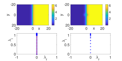
Figure 2: (Color online) The top panels show examples of the sG kinks with a radial external potential of the form $V_{\rm ext}(r)=A\,{\rm sech}(r)$. The left panels are for $A=0$ (i.e., in the absence of the potential for a “standard” 2D sG model), while the right panels are for $A=-4$. The bottom panels show the eigenvalues associated with the kinks in the linearized stability analysis. In the bottom left panel, the numerically computed eigenvalues from the full system (33) (blue circles) are found in excellent agreement with the theory (red stars), see Eq. (18) with $A=0$, namely $\lambda=ik\pi/L_{y}$.

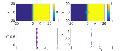
Figure 3: (Color online) Exactly the same panels as with Fig. 2, and with exactly the same potential (and for the cases $A=0$ (left) and $A=-4$ (right)), but now for the $\phi^{4}$ model, to illustrate the generic nature of our findings.

We observe in Fig. 2 that both the $A=0$ and $A=-4$ cases are dynamically stable with all of the corresponding eigenvalues on the imaginary axis. Furthermore, as evidenced in the bottom-left panel of Fig. 2, our approach captures the entire spectrum of the linearization around the coherent structure. Indeed, for $A=0$, all the modes predicted by the theory are identified in the stability analysis in excellent agreement between the two. In the $\phi^{4}$ case, see Fig. 3, the picture is rendered somewhat more complex due to the presence of the internal mode at $\omega=\pm\sqrt{3}$. Nevertheless, in addition to the continuous spectrum which in this case is for $\omega\in[2,\infty)$, we can notice the excellent matching between theory and numerics for the undulational modes of the unperturbed kink. To offer some perspective on the fact that such planar kinks can even be perturbed —without being destabilized— in the non-longitudinal direction, we have included a radial potential of the form $V_{\rm ext}(r)=-4\,{\rm sech}(r)$. As depicted in Figs. 2 and 3, the kink remains stable after the addition of this radial potential, solely incurring a small deformation in the vicinity of its center in the area of action of the heterogeneous external potential.

Figure 4: (Color online) An example of the sG model with a longitudinal potential $V_{\rm ext}(x)=A\,{\rm sech}^{2}(x)$ that conforms to the kink symmetry. Importantly, this potential renders the kink immediately unstable. The case example of $A=0.25$ is shown in the top panel for the kink profile, while the bottom shows the corresponding eigenvalues as computed numerically (blue circles) and as calculated by the analytical theory (red stars), see Eq. (18).

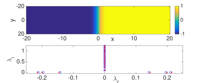
Figure 5: (Color online) Exactly the same panels as with Fig. 4, and with exactly the same potential but now for the $\phi^{4}$ model, and specifically for $A=0.1$. Theoretical values (red stars) are estimated from Eq. (19).

Now, to touch base with the theory developed in the previous section, we examine a case in which the potential is along the longitudinal direction and is of the form $V_{\rm ext}(x)=A\,{\rm sech}^{2}(x)$. Notice that now Eqs. (16) and (17), respectively, apply for the sG and $\phi^{4}$ models. Furthermore, more practically related to the computations in Figs. 4 (for sG) and 5 (for $\phi^{4}$), Eqs. (18) and (19) are applicable. From these, we see immediately that the selection of a value of $A>0$ will lead to instability for all values of $A\neq 0$, while a choice of $A<0$ will lead to spectral stability. Indeed, we consider in the cases of Figs. 4 and 5, particular examples of instability, in order to test the validity of the theory and its ability to capture both the unstable and also the stable modes of the solitonic filament. In both cases, we see that the eigenvalue predictions of Eqs. (18) and (19) are generally in very good agreement with the theory (although the theory slightly overestimates the corresponding growth rates).

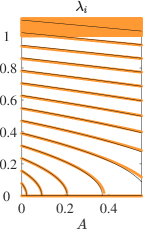
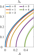
Figure 6: (Color online) Stability spectra for the sG model as a function of the amplitude of the longitudinal potential $V_{\rm ext}(x)=A\,{\rm sech}^{2}(x)$. The left, middle, and right panels depict, respectively, $\lambda^{2}$, $\lambda_{i}={\rm Im}(\lambda)$, and $\lambda_{r}={\rm Re}(\lambda)$. The thick colored lines corresponds to the numerically computed spectra and the thin black lines to our theoretical predictions given by Eq. (18). Note that for the unstable modes (see the right panel) the different $k$-modes have been identified.

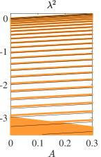
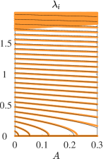
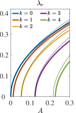
Figure 7: (Color online) Same as in Fig. 6 but for the $\phi^{4}$ model. Theoretical predictions are given by Eq. (19).

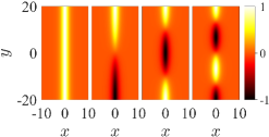
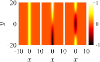
Figure 8: (Color online) Unstable eigenfunctions for the sG (left group of panels) and the $\phi^{4}$ (right group of panels) models corresponding to the steady states shown in Figs. 4 and 5 in the presence of the longitudinal potential $V_{\rm ext}(x)=A\,{\rm sech}^{2}(x)$ for $A=0.25$ and $A=0.1$, respectively. Note that for these parameter values, the steady state for the sG model possesses four unstable eigenvalues ($k=0$, $k=1$, $k=2$, and $k=3$) while for the steady state for the $\phi^{4}$ model has three unstable eigenvalues ($k=0$, $k=1$, and $k=2$).

To get a better sense of the theory’s capability at predicting the stability of the corresponding kinks in the presence of external potentials, we depict in Figs. 6 and 7 the linearization spectra as the amplitude $A$ of the longitudinal potential $V_{\rm ext}(x)=A\,{\rm sech}^{2}(x)$ is varied. As can be seen, overall, both in the absence of a potential and in the presence of a longitudinal one, the theory yields the correct qualitative and a good quantitative picture for the existence and stability of the kink. This predisposes us to believe that the AI approach might also give an accurate description of the full, nonlinear, dynamics of the kink filament. It is important to note that the theory allows us to obtain an immediate sense of whether the kink will be stable or unstable (and how unstable, if it is indeed unstable).

Let us now focus on the dynamics of the kinks. As detailed above, in the presence of the external potential $V_{\rm ext}(x)=A\,{\rm sech}^{2}(x)$, the stationary kink becomes immediately unstable for $A>0$. The dynamics of this instability will be mediated by the presence of eigenfunctions associated with unstable eigenvalues. In Fig. 8 we plot the unstable eigenfunctions corresponding to the case presented in Figs. 4 and 5. These unstable eigenfunctions will dictate the initial destabilization of the steady states. Note that for both, the sG and the $\phi^{4}$ cases, the $k=0$ and $k=1$ modes have very similar corresponding eigenvalues. Therefore, we expect the destabilization dynamics to follow, predominantly, a combination of these two modes. Note that given the form of the perturbation expansion in Eq. (32), the eigenfunctions should also be used to construct suitable perturbations of the velocity field at $t=0$ according to $u_{t}(x,y,t)=\epsilon\lambda e^{\lambda t}w(x,y)$. Thus, in Fig. 8 a light region indicates movement to the right while a dark region indicates movement to the left (or vice versa). As such, the first unstable ($k=0$) mode for each model corresponds to a translational mode that destabilizes the kink and makes it go “down the hill” from the external potential. The next mode, associated with $k=1$, will cause the kink to snake such that half of it goes to the right and the other half goes to the left of the external potential hill (or vice versa). Similarly, other (higher) unstable modes will induce snaking of the kink according to the wavenumber $k$.

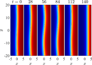
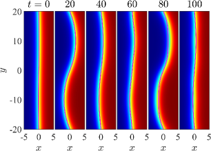
Figure 9: (Color online) Dynamics of a sG kink under the longitudinal potential $V_{\rm ext}(x)=A\,{\rm sech}^{2}(x)$ for $A=0.1$ (top panels) and $A=0.25$ (bottom panels) at the indicated times. The background image depicts the field $u(x,y,t)$ while the magenta line depicts the corresponding dynamics using the reduced AI PDE (15) with $P^{\prime}(X)$ defined in Eq. (16). Both systems are initialized with the same initial condition corresponding to a stationary kink perturbed with the $k=2$ longitudinal mode with amplitude 0.1. Namely, the initial location of the kink is given by $X(y,t=0)=\varepsilon\,\sin(\pi ky/L_{y})$ with $\varepsilon=0.1$ and $k=2$. See Supplemental Material movie-sG-1 and movie-sG-2 for animations depicting the corresponding dynamics SupMat .

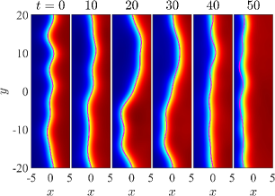
Figure 10: (Color online) Same as in Fig. 9 but for $A=0$ (top panels) and $A=0.25$ (bottom panels) for an initial condition corresponding to a stationary kink perturbed with a (linear) combination of the modes $k=2,4,6,8,10$. Specifically, $X(y,t=0)=\sum_{j=1}^{5}\varepsilon_{j}\,\sin(2\pi jy/L_{y}+\varphi_{j})$ with $\varepsilon_{j}=0.3$, $\varphi_{j}=(j-1)L_{y}\pi/10$, and $k=2j$. See Supplemental Material movie-sG-3 and movie-sG-4 for animations depicting the corresponding dynamics SupMat .

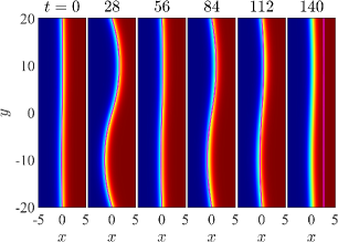
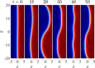
Figure 11: (Color online) Same as in Fig. 9 but for the $\phi^{4}$ model. See Supplemental Material movie-phi4-1 and movie-phi4-2 for animations depicting the corresponding dynamics SupMat .

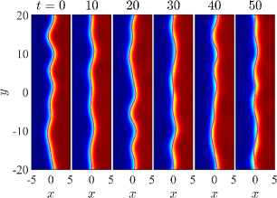
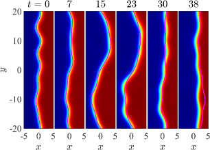
Figure 12: (Color online) Same as in Fig. 10 but for the $\phi^{4}$ model. See Supplemental Material movie-phi4-3 and movie-phi4-4 for animations depicting the corresponding dynamics SupMat .

So far, we have shown that the AI does a very good job at predicting the linearized behavior around the steady state. Therefore, at this stage, we would like to directly compare the full (nonlinear) dynamics of the sG and $\phi^{4}$ kinks to that predicted by our AI reduction. Figure 9 shows a comparison, for a couple of cases, between the full sG dynamics and the reduced AI PDE (15) with $P^{\prime}(X)$ defined in Eq. (16). As can be observed, the AI reduction is able to predict the full nonlinear dynamics of the kink. In particular in these two cases, the dynamics is a combination of the oscillations of the $k=2$ mode and the destabilization through the translational $k=0$ mode. Further numerical experiments (not shown here) show that this combined dynamics is rather general for a wide range of initial conditions of the kink of the form $X(y,t=0)=\varepsilon\,\sin(\pi ky/L_{y})$ for $k>0$ (or combinations thereof for different values of $k$). Namely, the typical dynamics is one where the different $k$ modes are initially destabilized according to their unstable eigenvalue (see the linear stability results above) and as they grow they enter the nonlinear regime of the dynamics and appear to return to the vicinity of the initial stationary kink. At the same time, perturbations along the $k=0$ (translational) mode —seeded by the initial condition or numerically seeded by the finite precision of the numerics— push the kink completely to one side of the crest of the longitudinal external potential. Then the kink continues to oscillate along the perturbed $k>0$ modes while it has gained horizontal (in the $x$-direction) speed and keeps traveling towards the boundary of the domain. In Fig. 10 we further test the capability of the reduced AI PDE in predicting the full sG dynamics by initializing the kink with a perturbation that includes a (linear) combination of the modes $k=2,4,6,8,10$ in the absence (top panels) and presence (bottom panels) of the longitudinal potential. In the absence of an external potential the kink is (neutrally) stable, and as such it only “wiggles” in a linear fashion [i.e., each of the $k$ modes oscillates according to its frequency given by Eq. (18)]. Perhaps more interesting is the dynamics under the influence of the longitudinal potential as the lowest-lying modes (in this case $k=0,1,2,3$) are unstable. In this case, as seen in the bottom panels of Fig. 10, the dynamics is more involved as it is fully nonlinear. Nevertheless, the AI reduction is able to closely emulate the dynamics of the full system even in this fully nonlinear regime.

Finally, in Fig. 11 and 12 we present the equivalent results to those presented in Figs. 9 and 10 but for $\phi^{4}$. As it could be anticipated, the AI reduced model is also able to predict the full $\phi^{4}$ dynamics not only in the linear regime but also in the fully nonlinear regime for considerably long times. Nevertheless, the slight deviations identified in the instability growth rates will eventually affect the quantitative matching between the two for sufficiently long time scales as can be seen in these figures.

III.2 Radial KG Kinks

We now turn to the case of the radial kinks. Here the theory provides a very useful guideline about inducing an unprecedented (to the best of our knowledge) steady state radial kink. Namely, the analytical results serve to guide the intuition of how to select an effective potential that counters the inward force exerted on the kink by curvature. In so doing, this ring potential succeeds in stabilizing the kink against this inward collapse and allows it to execute stable oscillations around the selected equilibrium position. Moreover, the theory serves to explain the fact that the azimuthal undulations do not destabilize the kink but simply correspond to stable oscillatory modes (akin to Kelvin waves in the BEC realm siambook ). Indeed, everything once again seems to be entirely the opposite of the defocusing NLS case (confirming a similarity to a focusing rather than a defocusing nonlinearity). In particular, in repulsive atomic BECs described by defocusing NLS, the curvature pushes the dark solitons outward, while the trap induces them a restoring force enabling the equilibrium. Around this equilibrium, the undulations are unstable, leading to the formation of vortices djf ; siambook . For the KG case however, the inward effect of curvature is countered, as is shown in Figs. 13 (for sG) and 14 (for $\phi^{4}$), by a suitable external potential. In the latter setting the undulations are purely oscillatory and the radial state is spectrally stable.

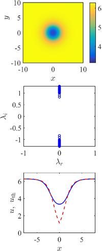
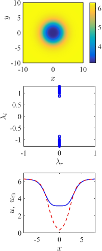
Figure 13: (Color online) Stationary radial kink for the sG model under and external potential of the form $V_{\rm ext}(r)=A\,{\rm sech}(r)$. The top two sets of panels correspond to $A=-6$ (left) and $A=-16$ (right). The top panels show the two-dimensional radial kink solution, while the middle panels confirm that these solutions are dynamically stable by showing their spectrum (residing on the imaginary axis). The bottom panels compare the exact numerical solution (solid blue line) with the theoretical prediction $u_{\rm th}$ (red dashed line) for such an equilibrium given by a sG kink centered at $R_{0}$ given by solving Eq. (26). The corresponding theoretical values for the equilibrium radius are $R_{0}=1.2212$ for $A=-6$ and $R_{0}=2.4541$ for $A=-16$.

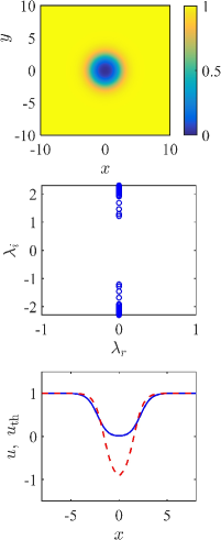
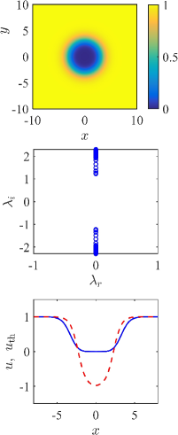
Figure 14: (Color online) Exactly the same diagnostics as for the sG equation and for the same potential but now for the case of the radial potential in the $\phi^{4}$ model. The corresponding theoretical values for the equilibrium radius from Eq. (26) are $R_{0}=1.5565$ for $A=-6$ and $R_{0}=2.2812$ for $A=-16$.

Using the information provided by the AI analysis of Sec. II.3, we searched for a stationary solution of the radial Klein-Gordon equation

$$u_{tt}=u_{rr}+\frac{1}{r}u_{r}-(1+V_{\rm ext})V^{\prime}(u)=0,$$ (34)

using Newton iterations. Explicitly, the Newton iteration to obtain the next iterate $u^{n+1}$ in terms of the current iterate $u^{n}$ can be cast as

$$\left[\partial_{rr}+\frac{\partial_{r}}{r}-(1+V_{\rm ext})V^{\prime\prime}(u^{n})\right]u^{n+1}$$

$$\qquad\qquad=(1+V_{\rm ext})\left[V^{\prime}(u^{n})-V^{\prime\prime}(u^{n})\,u^{n}\right],$$

where $u^{0}$ is a small radial Gaussian initial guess. The problem is discretized using finite differences where at $r=0$ we use l’Hôspital’s rule to regularize the term $u_{r}/r$. As may be expected we obtain no steady states for $A>0$. However, for $A<0$, we obtain rapid convergence to the profiles shown in the top panels of Figs. 13 and 14. As $A$ is decreased, the solution at $r=0$ tends to $\pi$ for the sine-Gordon equation ($0$ for $\phi^{4}$) where it asymptotes. The central flat region where $u\approx\pi$ then increases its extent as $A$ decreases further.

In the bottom panels in Figs. 13 and 14 we compare the prediction (with a red dashed line) of the theoretical radial equilibrium state of Sec. II.3 against the full numerical finding of the corresponding computation (in a blue solid line) for the potential $V_{\rm ext}$ given by the (magenta) dash-dotted line. We can see that the theory only does a moderately accurate job of capturing the ring equilibrium. However, a closer inspection clarifies why this is rather natural to expect to be the case. The equilibrium radius is rather small (i.e., between 1 and 2.5 in the cases shown in the figures). In such a setting, the ansatz used is not sufficiently accurate, as the approximations that we made in reaching the filament PDEs are not valid. In that sense, it is already quite encouraging that despite the lack of validity of its assumptions, the theory does a fairly reasonable job in capturing —even if only in a sort of averaged sense— the rough profile and location of the actual steady state kink. It is important to note in this context that we also tried to examine cases of much stronger potentials (cf., e.g., the top right panels in each of Figs. 13 and 14). In this case, an intriguing phenomenon arises that merits further study. In particular, indeed the kink widens as is expected from the theory since the force stemming from the potential (which stabilizes against the inward curvature induced motion) increases. However, instead of reaching all the way to $0$ for $r\approx 0$, as a 1D kink would, the kink widens towards $\pi$ and then flattens there (this is for the sG case —an analogous feature happens for $\phi^{4}$ with the $u=0$ state). It is remarkable that the saddle point presents a form of “impenetrable barrier” and the kink ends up forming in the radial setting between $\pi$ and $2\pi$ for sG and between $0$ and $1$ for $\phi^{4}$. Once again, this warrants further investigation and the potential use of a suitably adapted ansatz to this setting.

For the purposes of the present work, we offer a qualitative energetic argument about the existence of this state. At the level of Eq. (22), for a stationary radial state, the first (kinetic) and third (angular variation) terms in the energy are absent. If, then, there is a connection between two different steady states, the homogeneous (i.e., independent of $V_{\rm ext}$) fraction of the energy contributing to such a state is given by

$$E_{\rm rad}^{\rm 1K}=2\pi\int_{0}^{\infty}r\left[\frac{1}{2}u_{r}^{2}+V(u)\right]\,dr.$$ (35)

In the limit of a potentially very thin kink centered at $r=R$, this energy can be approximated as

$$E_{\rm rad}^{\rm 1K}\approx 2\pi R\,E_{\rm 1D}^{\rm 1K},$$

where now $E_{\rm 1D}^{\rm 1K}$ is the quasi-1D energy of this radial coherent structure. However, this energetic contribution “by itself” is minimized at an $R=0$ radius, i.e., there is no term to balance it and hence no such kink can arise without the presence of an external potential term. On the other hand, the inner state is at the saddle value $u=u_{s}$ (where $u_{s}=\pi$ for the sG model and $u_{s}=0$ for the $\phi^{4}$ model), with positive energy $V(u_{s})>0$ [$V(u_{s})=2$ for the sG model and $V(u_{s})=1/2$ for the $\phi^{4}$ model]. Furthermore, if $V_{\rm ext}$ is non-zero (and, more specifically, negative to offer a balancing energetic contribution), then there also exists a “bulk” energetic contribution of the form:

$$E_{\rm rad}^{\rm ext}\approx 2\pi\int_{0}^{\infty}rV_{\rm ext}(r)V(u)\,dr.$$ (36)

In the limit of a thin filament of radius $r=R$, and if we have defined the $V(u=0)=V(2\pi)=0$ for sG [similarly $V(\pm 1)=0$ for $\phi^{4}$], this energy can be approximated as:

$$E_{\rm rad}^{\rm ext}=2\pi V(u_{s})\int_{0}^{R}rV_{\rm ext}(r)\,dr.$$ (37)

This becomes even simpler if, e.g., $V_{\rm ext}$ is a potential well of depth $V_{0}$ in which case the integral simplifies further as

$$E_{\rm rad}^{\rm ext}\approx-V(u_{s})V_{0}\pi R^{2},$$

which is clearly indeed a bulk contribution. We can now add the approximate surface and bulk expressions obtained above, take the extremum and obtain the approximate equilibrium radius

$$R_{0}\approx\frac{E_{\rm 1D}^{\rm 1K}}{V(u_{s})V_{0}}.$$

This approximation is in the ballpark of our numerical findings and offers some insight towards the energetic balance that gives rise to the existence of this stable radial kink.

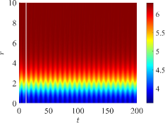
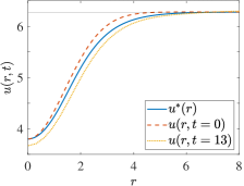
Figure 15: (Color online) An example of the oscillatory radial evolution dynamics of the initial condition of Eq. (38) for the radial PDE of Eq. (10) and $V_{\rm ext}(r)=-4\,{\rm sech}(r)$. The left panel shows the $(r,t)$ space-time contour plot illustrating the stable vibrating dynamics of the radial kink. The right panel portrays individual cuts involving the state at $t=0$ (orange dashed) and the result at $t=13$ (yellow dotted; this time is denoted by a vertical line on the left panel). For comparison the exact stationary, stable radial configuration is depicted by a blue solid line.

The stability of this radial kink was also tested dynamically whereby we used the steady state kink (depicted by a blue solid line in the right panel of Fig. 15) as the initial condition of a time dependent radial sine-Gordon code (see Ref. caputo for the details on the numerics). We observed no significant deviation of the profile for times up to $t=3000$, indicating dynamical stability. Furthermore, we also provided a larger perturbation of the kink by initializing the system with the profile

$$u(r,0)=\pi(2-0.79)\exp\left(-\frac{r^{2}}{4}\right),\quad u_{t}(r,0)=0.$$ (38)

depicted by a red dashed line in the right panel of Fig. 15. We see that despite the perturbed form of the initial condition, the radial kink remains “trapped” in the effective potential well of its radial energy landscape, oscillating robustly around the stable minimum corresponding to the stationary, stable configuration identified above. These results corroborate our spectral stability analysis.

IV Conclusions & Future Work

In the present work, we have explored a variety of settings related to the transverse dynamics of kinks in KG models. We started from the realm of planar (one-dimensional along, say, the $x$-direction) kinks in a 2D domain. We illustrated the stability of such structures against transverse undulations in the realm of the adiabatic invariant theory of solitonic filaments. Subsequently, we introduced external potentials of different types (radial or longitudinal) and explored under which conditions they could lead to stability or immediate instability of the original kink structures. Not only did we identify the qualitative conclusion regarding this stability question; we also provided a systematic set of predictions for the eigenvalues associated with the transverse undulations of the kink. Even beyond that, we have given an equation that describes the genuine nonlinear dynamics of the kink as a solitonic filament embedded within the 2D space.

We then turned to the case of radial kinks. So far, in this setting the attempts have been to observe and characterize the detrimental motion of the kink inward as induced by the $1/R$ effect of curvature. The most recent attempt was to utilize this phenomenon as a source of fast breathers. The present work moves one step further offering, on the basis of practically accessible spatial inhomogeneities, the ability to produce a force countering the curvature and producing a stationary stable radial kinklike structure.

Nevertheless, there are numerous challenges that the present work raised towards future studies that are worthy of further consideration. In the realm of longitudinal structures, it would be interesting to explore whether not only longitudinal potentials, but also more general ones (such as those used in the right panels of Figs. 2 and 3 could be addressed within the theory. In principle the theory does provide this possibility at the level of the center of the structure considerations given herein. However, the above figures suggest that perhaps using ansätze with further variables (such as the kink width) may be more suitable to tackle such a setting.

A perhaps wider range of challenges awaits regarding the radial kink case. Here, the adiabatic invariant formulation provides a useful guideline but not a quantitative diagnostic. Extending the theoretical considerations beyond the limitations and assumptions detailed herein is a significant challenge that is certainly worthy tackling. However, even at the purely numerical level (and at the level of associated mathematical analysis) there are surprises here. Perhaps the predominant one in this vein is the feature identified in both the sG and $\phi^{4}$ models, whereby as the potential strength is enlarged, a coherent structure is created connecting the former saddle point (e.g. $u=\pi$ in sG or $u=0$ in $\phi^{4}$) with the asymptotic value (of $u=2\pi$ in sG or $u=\pm 1$ in $\phi^{4}$). It is as if this saddle point operates as an impenetrable barrier for the asymptotics of the state in such a higher dimensional setting. This clearly merits some theoretical understanding, further numerical exploration and potentially a modified adiabatic invariant theory utilizing a suitable structure for such an asymptotic state.

Additionally, one can envision numerous further generalizations, including the consideration of general (rather than purely radially symmetric) potentials in 2D, as well as the promising extension of the present considerations in planar, spherical or more complex 3D patterns. Such studies are presently in progress and will be reported in future publications.

- (1) Y. S. Kivshar and G. P. Agrawal, Optical Solitons: From Fibers to Photonic Crystals (Academic, San Diego, 2003).
- (2) L. P. Pitaevskii and S. Stringari, Bose-Einstein Condensation. Oxford University Press (Oxford, 2003).
- (3) P. G. Kevrekidis, D. J. Frantzeskakis, and R. Carretero-González, The defocusing nonlinear Schrödinger equation: from dark solitons and vortices to vortex rings (SIAM, Philadelphia, 2015).
- (4) E. A. Kuznetsov and S. K. Turitsyn, Zh. Eksp. Teor. Fiz. 94, 119–129 (1988) [Sov. Phys. JETP 67, 1583–1588 (1988)].
- (5) Yu. S. Kivshar and D. E. Pelinovsky, Phys. Rep. 331, 117–195 (2000).
- (6) L. M. Pismen, Vortices in Nonlinear Fields (Clarendon, UK, 1999).
- (7) Yu. S. Kivshar and B. Luther-Davies, Phys. Rep. 298, 81–197 (1998).
- (8) D. J. Frantzeskakis, J. Phys. A: Math. Theor. 43, 213001 (2010).
- (9) V. Tikhonenko, J. Christou, B. Luther-Davies, and Yu. S. Kivshar, Opt. Lett. 21, 1129–1131 (1996).
- (10) B. P. Anderson, P. C. Haljan, C. A. Regal, D. L. Feder, L. A. Collins, C. W. Clark, and E. A. Cornell, Phys. Rev. Lett. 86, 2926–2929 (2001).
- (11) V. A. Mironov, A. I. Smirnov, and L. A. Smirnov, Zh. Eksp. Teor. Fiz. 139, 55 (2011) [Sov. Phys. JETP 112, 46 (2011)].
- (12) M. A. Hoefer and B. Ilan, Phys. Rev. A 94, 013609 (2016).
- (13) P. G. Kevrekidis, W. Wang, R. Carretero-González, and D. J. Frantzeskakis, Phys. Rev. Lett. 118, 244101 (2017).
- (14) P. G. Kevrekidis, Wenlong Wang, R. Carretero-González, and D. J. Frantzeskakis Phys. Rev. A 97, 063604 (2018)
- (15) M. Ma, R. Carretero-González, P. G. Kevrekidis, D. J. Frantzeskakis, and B. A. Malomed, Phys. Rev. A 82, 023621 (2010) and references therein.
- (16) Yu. S. Kivshar and X. Yang, Phys. Rev. E 50, R40 (1994).
- (17) D. Neshev, A. Dreischuh, V. Kamenov, I. Stefanov, S. Dinev, W. Fliesser, and L. Windholz, Appl. Phys. B 64, 429 (1997); A. Dreischuh, D. Neshev, G. G. Paulus, F. Grasbon, and H. Walther, Phys. Rev. E 66, 066611 (2002).
- (18) T. P. Horikis and D. J. Frantzeskakis, Opt. Lett. 41 583–586 (2016).
- (19) G. Theocharis, D. J. Frantzeskakis, P. G. Kevrekidis, B. A. Malomed, and Yu. S. Kivshar, Phys. Rev. Lett. 90, 120403 (2003).
- (20) G. Theocharis, P. Schmelcher, M. K. Oberthaler, P. G. Kevrekidis, and D. J. Frantzeskakis, Phys. Rev. A 72, 023609 (2005).
- (21) L. A. Toikka, J. Hietarinta, and K.-A. Suominen, J. Phys. A: Math. Theor. 45, 485203 (2012).
- (22) L. D. Carr and C. W. Clark, Phys. Rev. A 74, 043613 (2006).
- (23) W. Wang, P. G. Kevrekidis, R. Carretero-González, and D. J. Frantzeskakis, Phys. Rev. A 93, 023630 (2016).
- (24) N. S. Ginsberg, J. Brand, and L. V. Hau, Phys. Rev. Lett. 94, 040403 (2005).
- (25) J. Cuevas, P. G. Kevrekidis, F. L. Williams (Eds.), The sine-Gordon Model and its Applications: From Pendula and Josephson Junctions to Gravity and High Energy Physics, Springer-Verlag, (Heidelberg, 2014).
- (26) G. Parisi, Statistical Field Theory, Addison-Wesley (New York, 1988).
- (27) D. K. Campbell, J. F. Schonfeld, C. A. Wingate, Phys. 9D, 1 (1983).
- (28) T. I. Belova and A. E. Kudryavtsev, Phys. Usp. 40, 359 (1997).
- (29) Yu. S. Kivshar and B. A. Malomed Rev. Mod. Phys. 61, 763 (1989).
- (30) P. L. Christiansen, O. H. Olsen, Phys. Scr. 20, 531 (1979); P. L. Christiansen, O. H. Olsen, Phys. Lett. A 68, 185 (1978); P. S. Lomdahl, O. H. Olsen, P. L. Christiansen, Phys. Lett. A 78, 125 (1980); P. L. Christiansen, P. S. Lomdahl, Phys. 2D 482 (1981).
- (31) J. Geicke, Phys. 4D 197 (1982); J. Geicke, Phys. Scr. 29, 431 (1984); J. Geicke, Phys. Lett. A 98, 147 (1983).
- (32) I. L. Bogolubsky, V. G. Makhankov, JETP Lett. 24, 12 (1976).
- (33) M. R. Samuelsen, Phys. Lett. A 74, 21 (1979).
- (34) B. A. Malomed, Phys. 24D, 155 (1987).
- (35) B. A. Malomed and E. M. Maslov, Phys. Lett. A 160, 233 (1991).
- (36) M. Gleiser, D. Sicilia, Phys. Rev. D 80, 125037 (2009)
- (37) J.-G. Caputo and M. P. Soerensen, Phys. Rev. E 88, 022915 (2013).
- (38) P. L. Christiansen, N. Groenbech-Jensen, P.S. Lomdahl, and B. A. Malomed, Physica Scripta 55, 131–134 (1997).
- (39) G. S. Mkrtchyan and V. V. Schmidt, Solid State Commun. 30, 791 (1979).
- (40) J.-G. Caputo, N. Flytzanis, and M. Devoret, Phys. Rev. B 50, 6471 (1994).
- (41) V. V. Konotop and L. P. Pitaevskii, Phys. Rev. Lett. 93, 240403 (2004).
- (42) G. Reinisch, J. C. Fernandez, N. Flytzanis, M. Taki, and S. Pnevmatikos, Phys. Rev. B 38, 11284 (1988).
- (43) J.-G. Caputo, N. Flytzanis and M. Vavalis, Int. J. Mod. Phys. C 7, 191 (1996).
- (44) See Supplemental Material at http://link.aps.org/supplemental/XX.XXXX/ for movies showing the dynamics of the sG and and our AI reduction.