Thermal and quantum lattice fluctuations in Peierls chains

Abstract

The thermodynamic and spectral properties of electrons coupled to quantum phonons are studied within the spinless Holstein model. Using quantum Monte Carlo simulations, we obtain accurate results for the specific heat and the compressibility, covering the entire range of electron-phonon couplings and phonon frequencies. To this end, we derive an efficient estimator for the specific heat using the properties of the perturbation expansion. This allows us to quantitatively test the predictions of Tomonaga-Luttinger liquid theory as well as the widely used adiabatic approximation for low phonon frequencies. A comparison with the spectral functions of electrons and phonons reveals that the formation of polaron excitations as well as the renormalization of the phonon mode across the Peierls transition have a pronounced effect on the specific heat in the adiabatic regime.

I Introduction

In one-dimensional (1D) systems, the Peierls instability [1; 2] can drive a metal-insulator transition to a state with long-range charge-density-wave (CDW) order accompanied by a periodic lattice modulation. Experimental realizations of this phenomenon include quasi-1D materials such as TTF-TCNQ [3] or $\mathrm{K_{0.3}MoO_{3}}$ [4]. A closely related problem is the spin-Peierls transition [5] in, e.g., $\mathrm{CuGeO_{3}}$ [6]. Even if the competing electron-electron interaction is neglected, a reliable quantum-phonon description of such transitions remains challenging.

The specific heat $C_{\text{V}}$ is a key experimental probe for the Peierls transition. While containing less information than, e.g., excitation spectra, it is easy to measure and exhibits a peak or an anomaly at $T_{c}$ [7; 8; 9; 10; 11; 12]. Some compounds display a mean-field like step in $C_{\text{V}}$, whereas in other compounds the anomaly is strongly smeared out by fluctuations [13]. The specific heat is often dominated by phonon contributions and played a key role for the development of a quantum theory of lattice fluctuations [14]. Despite its experimental importance, accurate results for microscopic models with quantum phonons are rare.

Investigations of 1D models are motivated by the typically much larger intrachain interactions compared to interchain interactions, as evinced by the fact that $T_{c}$ is typically much smaller than the predicted mean-field value [13]. While interchain couplings are necessary for the observed finite-temperature phase transition [13], the physics is determined by the 1D chains above a crossover temperature. In 1D, the second-order phase transition at $T_{c}>0$ is replaced by a crossover, with long-range order only at $T=0$. The widely used mean-field approaches [1; 15] are exact for classical phonons (adiabatic limit) at $T=0$. In the latter, thermal fluctuation effects (including solitons [16]) can be captured qualitatively with fluctuating gap models [17; 18] and quantitatively with Monte Carlo simulations [19]. The specific heat has a characteristic peak at a temperature where coherent CDW correlations and a well-defined Peierls gap emerge [19].

Important insights into the effects of quantum lattice fluctuations on Peierls insulators have come from numerical methods such as exact diagonalization [20; 21; 22], quantum Monte Carlo (QMC) [23; 24; 25; 26; 27; 28], and the density-matrix renormalization group (DMRG) [29; 30; 31; 32; 33], as well as analytical and semi-analytical methods [34; 35; 36; 37; 38]. Importantly, quantum fluctuations can significantly renormalize or even destroy the Peierls state, allowing for a gapless Luttinger liquid phase and a Peierls quantum phase transition. The phase diagram of the spinless Holstein model considered here (Fig. 1) has been determined quite precisely from DMRG calculations [33; 32].

Combined descriptions of both quantum and thermal effects are particularly challenging but well motivated: for example in $\mathrm{CuGeO_{3}}$, the relevant phonon frequencies are comparable to the spin exchange constant [39]. Other materials (e.g., polyacetylene [16]) fall into the adiabatic regime of small but finite phonon frequency. QMC results of limited quality are available for the spin-Peierls case for selected parameters [26; 37]. Finite-temperature DMRG calculations—successfully carried out for fermionic systems [40; 41]—are so far inhibited by the large phonon Hilbert space. The determination of $C_{\text{V}}$ from QMC simulations is limited by long autocorrelations [42], large fluctuations, and Trotter discretization errors [43]. Whereas the thermodynamic Bethe ansatz is not applicable beyond the classical-phonon limit [44], the bosonization has been applied to study the effect of the coupling to quantum phonons in the Luttinger liquid phase [45].

Here, we present accurate numerical results for the thermodynamic properties of a 1D Holstein model across all different parameter regimes: adiabatic and nonadiabatic, as well as metal and Peierls insulator. Previous limitations are overcome by combining a recently developed directed-loop algorithm for retarded interactions [46] with the calculation of bosonic observables from the perturbation expansion [47]. In particular, the specific heat is calculated directly on lattices of $L=162$ sites. Moreover, we obtain results for the single-particle spectral functions of electrons and phonons for previously inaccessible system sizes and temperatures to explain the observed low-temperature features of $C_{V}$.

The article is organized as follows: We introduce the Holstein model in Sec. II and outline the QMC method used in Sec. III. Results are presented in Sec. IV and we conclude in Sec. V. In the Appendix, we derive a QMC estimator for the specific heat of the Holstein model.

II Model

To isolate the effect of quantum lattice fluctuations on the thermodynamics of 1D chains, we consider a minimal theoretical model. The Hamiltonian of the spinless Holstein model [48] is given by

$$\hat{H}=-t\sum_{i}\big{(}\hat{c}^{\dagger}_{i}\hat{c}^{\vphantom{\dagger}}_{i+1}+\mathrm{H.c.}\big{)}+\omega_{0}\sum_{i}\hat{b}^{\dagger}_{i}\hat{b}^{\vphantom{\dagger}}_{i}+g\sum_{i}\hat{Q}_{i}\hat{\rho}_{i}\,.$$ (1)

Here, $\hat{c}^{\dagger}_{i},\hat{c}^{\vphantom{\dagger}}_{i}$ ($\hat{b}^{\dagger}_{i},\hat{b}^{\vphantom{\dagger}}_{i}$) create/annihilate an electron (phonon) at lattice site $i$. The Holstein model consists of an electronic hopping term with amplitude $t$, Einstein phonons with frequency $\omega_{0}$, and a local coupling between the lattice displacement $\hat{Q}_{i}=(\hat{b}^{\dagger}_{i}+\hat{b}^{\vphantom{\dagger}}_{i})/\sqrt{2M\omega_{0}}$ and the fermion density $\hat{\rho}_{i}=(\hat{n}_{i}-1/2)$. In the following, we only consider the half-filled case with $\langle\hat{\rho}_{i}\rangle=0$ and define the dimensionless coupling constant $\lambda=g^{2}/(4M\omega_{0}^{2}t)$. Here, $M$ is the mass of the harmonic oscillators. We use $t$ as the unit of energy and set $\hbar=1$.

Figure 1 shows the ground-state phase diagram of the spinless Holstein model as determined from DMRG simulations [33; 32]. The Holstein model describes the quantum phase transition from a Tomonaga-Luttinger liquid (TLL) at $\lambda<\lambda_{c}(\omega_{0})$ to a Peierls CDW insulator with ordering wavevector $q=2k_{\text{F}}=\pi$ at $\lambda>\lambda_{c}(\omega_{0})$ [24; 33; 20; 22; 32]. At $\omega_{0}=0$, the ground state shows CDW order for any $\lambda>0$ and is exactly described by mean-field theory, whereas for $\omega_{0}>0$ and small $\lambda$, quantum lattice fluctuations destroy the ordered state and lead to a TLL phase. For $\omega_{0}\to\infty$, the spinless Holstein model maps to free fermions and is hence always metallic. The nonuniversal Luttinger parameters $K$ and $u$ have been determined by DMRG calculations; for any $\omega_{0}$, the electron-phonon interaction leads to a repulsive TLL with $K<1$ and a reduction of the charge velocity $u$, see Ref. [32] and references therein. For further details on the ground-state properties we refer to the review [49].

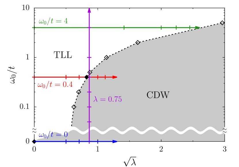
Figure 1: Ground-state phase diagram of the half-filled spinless Holstein model as a function of the electron-phonon coupling $\lambda$ and the phonon frequency $\omega_{0}$. Critical values are from DMRG calculations (open symbols) [33; 32]. Additionally, we show the QMC estimate $\lambda_{c}=0.68(1)$ at $\omega_{0}/t=0.4$ [46] and the exact value $\lambda_{c}=0$ at $\omega_{0}=0$ (filled symbols). Arrows indicate the paths in parameter space along which we discuss the thermodynamic properties of the Holstein model in this article. The simulation parameters are indicated by additional markers attached to the arrows. For explanations on the phase diagram see the main text.

While the DMRG yields critical values and Luttinger parameters, spectral or thermodynamic properties appear to be out of reach due to the large bosonic Hilbert space. Instead, spectral functions have been obtained from exact diagonalization [22] or QMC simulations [28; 47] on small system sizes as well as from analytic approaches [50; 36; 51]. Results for thermodynamic properties are only available in the adiabatic limit $\omega_{0}=0$ [19]. The effects of quantum lattice fluctuations have been studied for a spin-phonon model [26] but results are limited by the accessible temperature range and system sizes because only local QMC updates were available.

The spinless Holstein model captures the essential aspects of quantum Peierls chains while avoiding complications due to spin gap formation in the metallic phase that appear in the spinful case [52]. The phase transition from TLL to Peierls insulator is also very similar to the corresponding transition in the spinless Su-Schrieffer-Heeger model [53]. Moreover, for classical phonons, the two models exhibit a qualitatively very similar temperature dependence of the specific heat [19]. The Jordan-Wigner transformation provides a link between the spinless fermion model and spin-phonon models [54]. The choice of Einstein phonons (relevant for, e.g., $\mathrm{CuGeO_{3}}$ [55]) gives exponential rather than linear (for 1D acoustic phonons) behavior of $C_{\text{V}}$ at low temperatures. However, a low-energy theory reveals that only the $2k_{\text{F}}$ (zone-boundary) part of the phonon spectrum couples to the electrons [23; 56], and identical results have been reported for Su-Schrieffer-Heeger models with optical and acoustic phonons [38; 53]. Therefore, the decoupled part of the phonon spectrum merely contributes a trivial background to $C_{\text{V}}$ that is routinely subtracted from experimental data to reveal the interesting electron-phonon correlation effects.

III Method

To simulate the Holstein model, we used the directed-loop QMC method for retarded interactions in the stochastic series expansion (SSE) representation [46]. Starting from the coherent-state path integral, the phonons are integrated out analytically [57] to obtain the purely fermionic action

$$\mathcal{S}=\mathcal{S}_{0} -t\int_{0}^{\beta}d\tau\sum_{i}\left[\bar{c}_{i}(\tau)\,c_{i+1}(\tau)+\bar{c}_{i+1}(\tau)\,c_{i}(\tau)\right]$$

$$-2\lambda t\iint_{0}^{\beta}d\tau d\tau^{\prime}\sum_{i}\rho_{i}(\tau)\,P(\tau-\tau^{\prime})\,\rho_{i}(\tau^{\prime})\,.$$ (2)

The coupling between electrons and phonons leads to a density-density-type interaction nonlocal in imaginary time and mediated by the free-phonon propagator $P(\tau)$. The SSE representation [58] corresponds to an expansion of the partition function around $\mathcal{S}_{0}=\int d\tau\sum_{i}\bar{c}_{i}(\tau)\,\partial_{\tau}\,c_{i}(\tau)$. The resulting trace over Grassmann fields is then mapped to an expectation value of an operator sequence. By formally promoting the hopping terms to retarded interactions, we can formulate efficient global directed-loop updates from local update rules [59] in which the time dependence of $P(\tau)$ only enters the diagonal updates. For details on the Monte Carlo updates see Ref. [46] and its Supplemental Material. Electronic observables are calculated directly from the Monte Carlo configurations [60; 61]. Bosonic observables can be recovered from electronic correlation functions using sum rules derived with the help of generating functionals [47].

We study the thermodynamics of the Holstein model in terms of the specific heat

$$C_{V}=k_{\text{B}}\beta^{2}\left[\left\langle\hat{H}^{2}\right\rangle-\left\langle\hat{H}\right\rangle^{2}\right]$$ (3)

and the compressibility (we define $\hat{N}=\sum_{i}\hat{n}_{i}$)

$$\kappa=\frac{\beta}{L}\left[\left\langle\hat{N}^{2}\right\rangle-\left\langle\hat{N}\right\rangle^{2}\right]\,.$$ (4)

Here $\beta=1/(k_{\text{B}}T)$ is the inverse temperature. While $\kappa$ is obtained directly from the world-line configurations, the calculation of $C_{V}$ via Eq. (3) is complicated by the fact that the phonon fields have to be extracted from fermionic correlation functions. In the Appendix, we derive an efficient estimator to measure $C_{V}$ in $\mathcal{O}(n)$ operations by exploiting properties of the interaction expansion ($n$ denotes the expansion order) [47].

As a second approach, we also calculated $C_{V}$ from the total energy via the relation $C_{V}=\partial E(T)/\partial T$. Following Ref. [62], we fitted $E(T)$ to the functional form

$$E(T)=\int d\omega\,\omega\,\big{[}n_{\text{F}}(\omega,T)\,\rho_{\text{F}}(\omega)+n_{\text{B}}(\omega,T)\,\rho_{\text{B}}(\omega)\big{]}$$ (5)

which corresponds to a spectral decomposition into noninteracting fermionic and bosonic contributions $\rho_{\text{F}}$ and $\rho_{\text{B}}$, respectively. This ansatz is well-motivated for the electron-phonon model at hand—compare Eq. (8) and the discussion of spectral functions below—but the temperature dependence is considered to originate only from the Fermi and Bose functions $n_{\text{F}}$ and $n_{\text{B}}$. Given Monte Carlo data for $E(T)$, Eq. (5) represents an inverse problem that can be solved using the maximum entropy approach [62; 63]. The spectra obtained in this way do not have a physical meaning and only serve to fit $E(T)$ with a reasonable $\chi^{2}$. Then, $C_{V}(T)$ can be easily calculated from $\rho_{\text{F}}$ and $\rho_{\text{B}}$ by applying the temperature derivative to the Fermi and Bose functions in Eq. (5). The results obtained in this way are in good agreement with those from Eq. (3) over a large temperature range. However, for some parameters we observe poor convergence especially at low temperatures because the fitting ansatz becomes too restrictive. Therefore, we prefer the unbiased and hence superior covariance estimator for $C_{V}$ and include the continuous fits from $E(T)$ merely as a guide to the eye. As the covariance estimators for $C_{V}$ and $\kappa$ are subject to large statistical fluctuations, we restrict our simulations to $L=162$ lattice sites.

To interpret the low-temperature features of the thermodynamic observables, we also calculated the single-particle spectral functions of electrons and phonons with Lehmann representations

$$A(k,\omega)=\frac{1}{Z}\sum_{mn}e^{-\beta E_{m}}\big{(}1+e^{-\beta\omega}\big{)}\left|\braket{m}{\hat{c}^{\vphantom{\dagger}}_{k}}{n}\right|^{2}\delta(\omega-\Delta_{nm})\,,$$

$$B_{Q}(q,\omega)=\frac{M\omega_{0}^{2}}{Z}\sum_{mn}e^{-\beta E_{m}}\left|\braket{m}{\hat{Q}_{q}}{n}\right|^{2}\delta(\omega-\Delta_{nm})\,,$$ (6)

respectively. Here, $\ket{m}$ is a many-particle eigenstate of the Hamiltonian, $E_{m}$ the corresponding energy eigenvalue, and $\Delta_{nm}=E_{n}-E_{m}$. We obtained the spectral functions from the corresponding Green’s functions $G(r,\tau)=\langle\hat{c}^{\dagger}_{r}(\tau)\hat{c}^{\vphantom{\dagger}}_{0}(0)\rangle$ and $D_{Q}(r,\tau)=\langle\hat{Q}_{r}(\tau)\hat{Q}_{0}(0)\rangle$. The electronic Green’s function can be accessed directly during the construction of the directed loop [64]. In the simulation of retarded interactions, each Monte Carlo vertex already includes imaginary-time variables so that an additional mapping is not necessary. The phonon propagator can be inferred from the density structure factor $S_{\rho}(q,\mathrm{i}\Omega_{m})=\int_{0}^{\beta}d\tau\,e^{\mathrm{i}\Omega_{m}\tau}\sum_{r}e^{-\mathrm{i}qr}\langle\hat{\rho}^{\vphantom{\dagger}}_{r}(\tau)\hat{\rho}^{\vphantom{\dagger}}_{0}(0)\rangle$ via [65]

$$D_{Q}(q,\mathrm{i}\Omega_{m})=P_{\!+}(\mathrm{i}\Omega_{m})+4\lambda t\,P_{\!+}(\mathrm{i}\Omega_{m})^{2}\,S_{\rho}(q,\mathrm{i}\Omega_{m})\,.$$ (7)

Here, $\Omega_{m}=2\pi m/\beta$ are the bosonic Matsubara frequencies and $P_{\!+}(\mathrm{i}\Omega_{m})=\omega_{0}^{2}/(\omega_{0}^{2}+\Omega_{m}^{2})$ is the free phonon propagator. $S_{\rho}(q,\mathrm{i}\Omega_{m})$ can be calculated efficiently in the SSE representation [60; 61]. Finally, the spectral functions $A(k,\omega)$ and $B_{Q}(q,\omega)$ are obtained via stochastic analytic continuation [66; 67] using $G(k,\tau=0)$ and $D_{Q}(q,\tau=0)$ as sum rules.

The total energy and hence also the specific heat $C_{V}=\partial E/\partial T$ are directly related to the single-particle spectral functions. Using the equation of motion [68], we obtain the sum rule

$$E=\sum_{k}\int_{-\infty}^{\infty}d\omega\,\frac{\omega+\epsilon_{k}}{2}\,n_{\text{F}}(\omega)\, A(k,\omega)$$

$$+\sum_{q}\int_{-\infty}^{\infty}d\omega\,\omega\,n_{\text{B}}(\omega)\, B(q,\omega)\,.$$ (8)

Here, $\epsilon_{k}=-2t\cos k$ is the bare electronic dispersion and $B(q,\omega)=Z^{-1}\sum_{mn}e^{-\beta E_{m}}(1-e^{-\beta\omega})|{\braket{m}{\hat{b}_{q}}{n}}|^{2}\delta(\omega-\Delta_{nm})$ the bosonic spectral function defined from the second-quantized operators. In the noninteracting limit, we have $A(k,\omega)=\delta(\omega-\epsilon_{k})$ and $B(q,\omega)=[\delta(\omega-\omega_{0})-\delta(\omega+\omega_{0})]/2$, i.e., the temperature dependence of $C_{V}$ only arises from the distribution functions $n_{\text{F}}$ and $n_{\text{B}}$. For finite electron-phonon interactions also $A(k,\omega)$ and $B(q,\omega)$ change with temperature. Note that the interaction energy equally contributes to the fermionic and bosonic parts in Eq. (8). Whereas $A(k,\omega)$ has been previously studied by an exact numerical method over the entire range of temperatures for classical phonons [19] [where the bosonic part in Eq. (8) reduces to the classical result $Lk_{\text{B}}T$], the quantum case requires numerical analytic continuation and we focus on the low-temperature spectral functions characterizing the ground state.

IV Results

We will discuss the thermodynamic properties of the spinless Holstein model along the paths in parameter space indicated in Fig. 1. As a function of the electron-phonon interaction $\lambda$, we consider both the antiadiabatic regime with $\omega_{0}\gg t$ and the adiabatic regime with $\omega_{0}\ll t$. Because the physics of the Holstein model is very different in the two regimes, we calculate the spectral functions of electrons and phonons at low temperatures to explain the characteristic signatures that appear in the thermodynamic observables. A special case of the adiabatic regime is the limit $\omega_{0}=0$ where spectral functions have been calculated exactly at finite temperatures [19]. For completeness, we review the main results obtained in this limit. The effects of quantum lattice fluctuations on the specific heat of a Peierls chain are finally studied as a function of $\omega_{0}$ from low to high phonon frequencies.

IV.1 Polaron formation in the antiadiabatic regime

In the antiadiabatic regime $\omega_{0}\gg t$, the metallic TLL phase extends up to rather strong couplings $\lambda$, see Fig. 1. With increasing $\lambda$, the electrons first undergo a crossover to small polarons with a significantly enhanced effective mass due to the dressing with phonons, before ordering into a polaronic superlattice at $\lambda_{c}$ [22]. These effects can be characterized by the single-particle spectral functions of electrons and phonons, which were previously calculated numerically in the antiadiabatic regime using exact diagonalization [22] and a projective renormalization approach [51]. The electronic spectral function has also been obtained by the bosonization method [50].

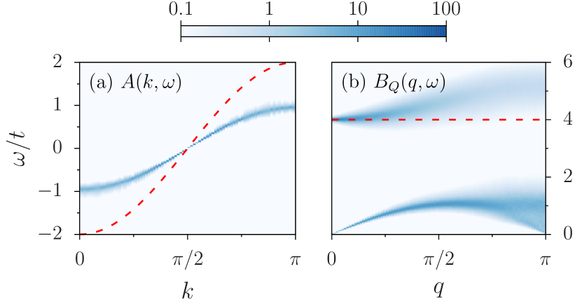
Figure 2: Single-particle spectral functions of (a) electrons and (b) phonons at $\omega_{0}/t=4$ and $\lambda=2$. Dashed lines indicate the corresponding free dispersions. Here, $L=162$ and $\beta t=2L$. Color scheme based on Ref. [69].

In Fig. 2, we present QMC results for $A(k,\omega)$ and $B_{Q}(q,\omega)$ for $\omega_{0}/t=4$ and $\lambda=2$ obtained for $L=162$ and $\beta t=2L$. The electronic spectrum in Fig. 2(a) exhibits a well-defined band with a renormalized cosine dispersion $-2\tilde{t}\cos k$ and $\tilde{t}=u/2$, with $u\approx 0.47\,v_{\text{F}}$ for the parameters considered. This polaronic renormalization (but not the Peierls transition at larger $\lambda$) can be qualitatively captured by the Lang-Firsov approximation [70; 71]. The renormalization of the electronic band is also visible in the phonon spectrum in Fig. 2(b). The lower branch of $B_{Q}(q,\omega)$ corresponds to the particle-hole continuum, which is visible in the phonon spectral function because of the density-displacement coupling in Eq. (1) and again reveals the renormalized electronic band. The upper branch starts at $\omega=\omega_{0}$ for $q=0$ and hardens with increasing $q$. The Peierls transition in the antiadiabatic regime is characterized as a central-mode transition, with a hardening of the phonon frequency and a central peak at $q=2k_{\text{F}}$ for $\lambda\geq\lambda_{c}$ [22].

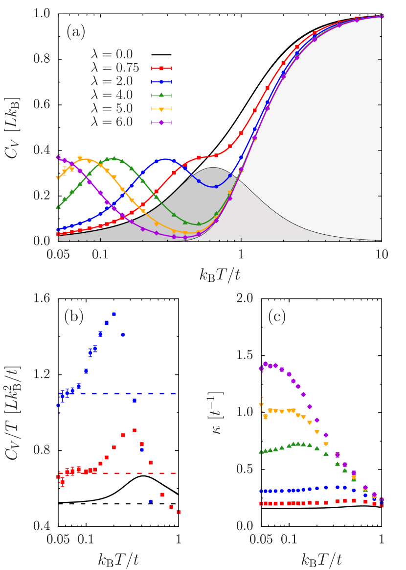
Figure 3: (a) Specific heat $C_{V}$, (b) specific heat over temperature $C_{V}/T$, and (c) compressibility $\kappa$ in the antiadiabatic regime ($\omega_{0}/t=4$, $L=162$). Data points correspond to direct estimates, whereas straight lines in (a) are obtained from fits to the total energy using the maximum entropy method. The shaded areas in (a) indicate the free-electron and free-phonon contributions to $C_{V}$. The dashed lines in (b) correspond to fits to the total energy of the form $E(T)=E_{0}+\frac{1}{2}aT^{2}$ in the interval $T\in[0.05,0.1]$.

To explore the thermodynamic signatures of the TLL phase, we follow the path in Fig. 1 at constant $\omega_{0}/t=4$ and $L=162$. At $\lambda=0$, the specific heat shown in Fig. 3(a) is the sum of two contributions. The free-phonon part approaches the Dulong-Petit law $C_{V}=Lk_{\text{B}}T$ for $T\to\infty$ but eventually drops off exponentially below $k_{\text{B}}T\approx\omega_{0}$. The free-electron part has a maximum at $k_{\text{B}}T\approx 0.63t$ that can be identified with the onset of coherent electronic motion [19].

The interpretation of the results in terms of electron and phonon contributions remains useful at $\lambda>0$. With increasing coupling, the high-temperature part of $C_{V}$ converges to the free-phonon contribution because the renormalization of the phonon branch in $B_{Q}(q,\omega)$ is smeared out by thermal fluctuations. At the same time, the formation of small polarons with substantially increased mass leads to a significant reduction of the effective hopping $\tilde{t}$, causing the electronic contribution to $C_{V}$ to shift towards lower temperatures while maintaining its shape. In particular, the temperature dependence of $C_{V}$ seems to originate mainly from the distribution functions in Eq. (8). Similar to $\lambda=0$, the low-temperature peak in $C_{V}$ can be identified with the onset of coherence, determined by the renormalized hopping $\tilde{t}$.

For the spinless model considered, there is a direct relation between the electronic contribution to $C_{V}$, the density of states at the Fermi level $N(E_{\text{F}})$, and the renormalized charge velocity $u$ [45; 72]. At temperatures where the phonon contribution is frozen out, we expect

$$C_{V}=\frac{\pi^{2}}{3}Lk_{B}^{2}T\,N(E_{\text{F}})=\frac{\pi}{3}\frac{Lk_{B}^{2}T}{u}\,.$$ (9)

The first expression is generic, the second expression holds in a TLL [45]. Figure 3(b) shows $C_{V}/T$ for the two smallest $\lambda$ considered. The convergence of $C_{V}/T$ for low $T$ to a constant that increases with $\lambda$ is clear evidence for the reduction of the charge velocity $u$. Low-temperature fits of the total energy to the form $E(T)=E_{0}+\frac{1}{2}aT^{2}$ are in good agreement with the $C_{V}$ data [cf. the dashed lines in Fig. 3(b)]. The reduction of $u$ can also be inferred from the compressibility shown in Fig. 3(c) whose low-temperature limit is given by [72]

$$\kappa=\frac{K}{u\pi}\,.$$ (10)

Equation (10) additionally includes the Luttinger parameter $K$ that also decreases with increasing $\lambda$. Comparing Fig. 3(c) with Fig. 3(a) reveals that the TLL regime with a constant $\kappa$ emerges below the coherence scale defined by the low-temperature peak in $C_{V}$. The observed decrease of $u$ with increasing $\lambda$ (reflecting the enhanced polaron mass) is in contrast to the $t$-$V$ model. The latter also has a critical point separating a TLL from a CDW insulator, but $u$ increases with increasing $V$ in the metallic phase [72] as recently also observed directly from thermodynamic properties [41]. The opposite behavior in electron-phonon models, namely a decrease of $u$ upon increasing the interaction, agrees with previous numerical [20; 33] and bosonization results [45].

IV.2 Formation of CDW order in the adiabatic limit

The previous section revealed the principal features of $C_{V}$ and $\kappa$ in the metallic phase. To understand the impact of quantum lattice fluctuations on the thermodynamic properties of Peierls insulators, we start from the adiabatic limit $\omega_{0}=0$ where they are entirely absent. Then, the ground state is a Peierls insulator for any $\lambda>0$ and exactly described by mean-field theory [1; 2]. The formation of a $2k_{\text{F}}$ CDW is accompanied by the opening of a single-particle gap and the formation of shadow bands due to the doubling of the unit cell [73; 19].

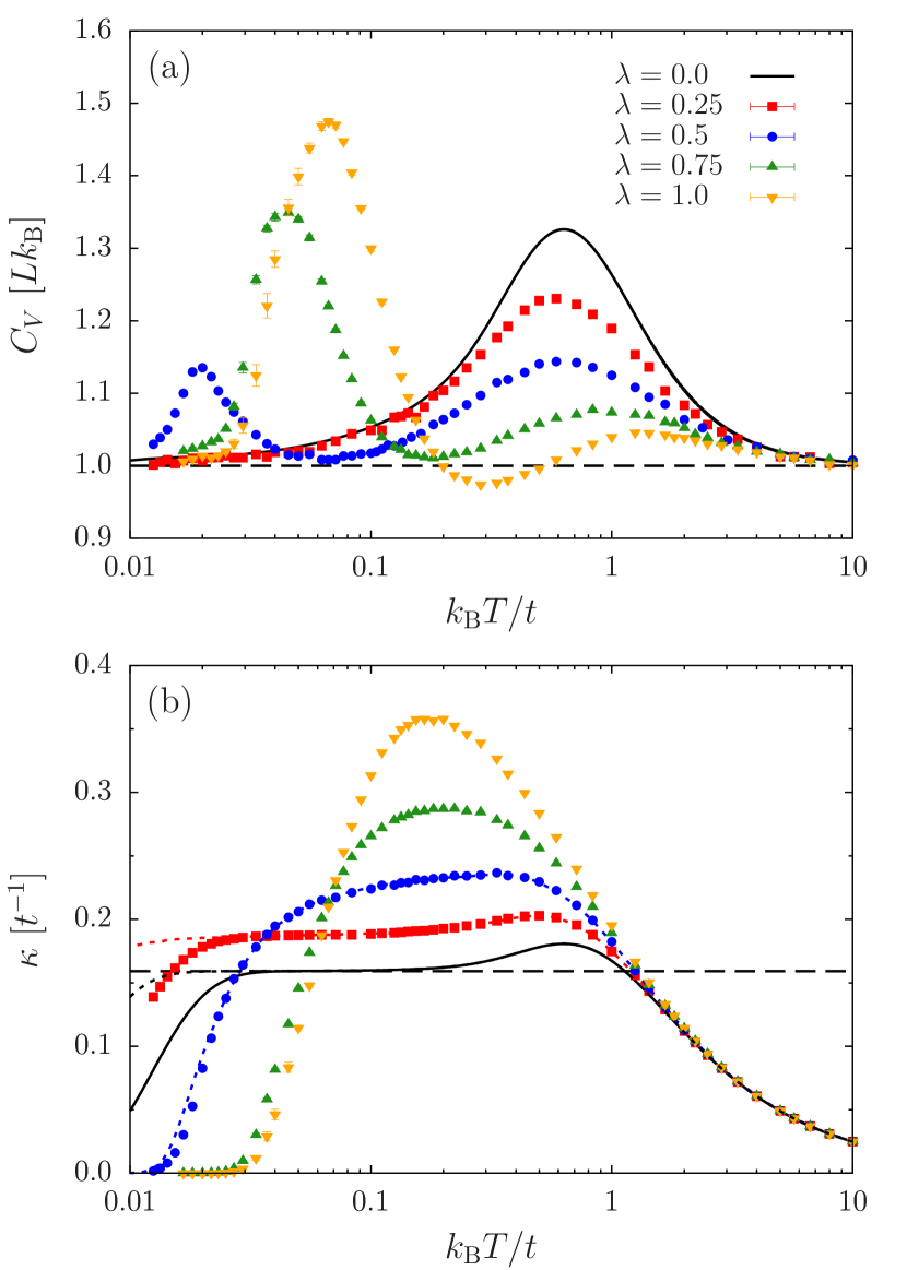
Figure 4: (a) Specific heat $C_{V}$ and (b) compressibility $\kappa$ at $\omega_{0}=0$. Dashed lines indicate the free-phonon contribution to $C_{V}$ and the $T=0$ limit of $\kappa$ at $\lambda=0$. Results were obtained using the Monte Carlo method of Ref. [74] for $L=162$. To illustrate finite-size effects for $\kappa$, we also show results for $L=322$ (short-dashed lines).

Thermal fluctuations in Peierls chains have been studied very generically in fluctuating gap models [17; 18] and recently also by QMC simulations of the classical Holstein model [19]. The latter approach permits the exact calculation of spectral properties without the need of numerical analytic continuation [74]. At $T>0$, the mean-field gap is filled in by polaron excitations bound to thermally generated domain walls [19]. The temperature scale where the gap disappears matches the position of a low-temperature peak in the specific heat [19]. According to Eq. (9), the low-temperature electronic contribution to $C_{V}$ scales directly with the density of states at $E_{\text{F}}$. Figure 4(a) shows $C_{V}$ for different electron-phonon couplings $\lambda$. While for $\lambda=0.25$ the peak related to the Peierls gap still lies outside the temperature range shown, it shifts to higher temperatures and grows with increasing $\lambda$, in accordance with the exponential opening of the gap. In contrast to the discontinuous feature predicted by mean-field theory, the peak in $C_{V}$ is smeared out by thermal fluctuations and appears at an energy scale much lower than the mean-field critical temperature [18]. At higher temperatures, $C_{V}$ again exhibits a peak related to the temperature scale where coherent band motion and Fermi statistics become relevant. With increasing $\lambda$, this peak is strongly suppressed. Whereas the Dulong-Petit law is obeyed at high temperatures, the classical phonons produce the same constant also at $T=0$, leading to the well-known violation of the third law of thermodynamics.

The formation of a pseudogap at low temperatures can also be inferred from the compressibility. Figure 4(b) reveals that $\kappa$ is suppressed at a temperature scale that matches the peak position in $C_{V}$. The sharp drop-off below $T\lesssim 0.02t$ visible in Fig. 4(b) for $\lambda=0$ and $\lambda=0.25$ is related to a finite-size gap, as illustrated by the results for $L=322$ (short-dashed lines). If the Peierls gap is sufficiently small, $\kappa$ exhibits the constant behavior characteristic of the TLL phase at intermediate temperatures. Apart from that, electron-phonon coupling enhances charge fluctuations at intermediate temperatures.

IV.3 Peierls transition in the adiabatic regime

Having established the thermodynamic signatures of the metallic and the insulating phase, we now consider the Peierls transition between these phases in the adiabatic quantum-phonon regime $0<\omega_{0}<t$. We will see that the evolution of the low-temperature specific heat across the transition is rather intricate due to impact of the electron and phonon dynamics. Therefore, we first review the corresponding single-particle spectral functions; a more detailed discussion can be found in Refs. [28; 65]. Specifically, Figures 5 and 6 show electron and phonon spectral functions for $\omega_{0}/t=0.4$ and different $\lambda$. The critical coupling for the Peierls transition is $\lambda_{c}=0.68(1)$ [46]. These results were obtained for $L=162$ and $\beta t=2L$, significantly larger than in previous works.

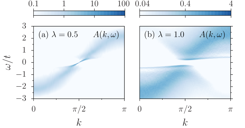
Figure 5: Electronic single-particle spectral function $A(k,\omega)$ in (a) the metallic phase and (b) the Peierls phase. Close-ups of the same results are presented in Fig. 6(b) and Fig. 6(d), respectively. Here, $\omega_{0}/t=0.4$, $L=162$, and $\beta t=2L$.

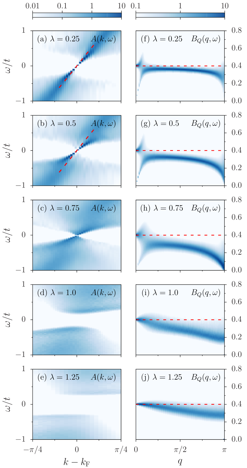
Figure 6: (a)–(e) Electronic single-particle spectral function $A(k,\omega)$ and (f)–(j) phonon spectral function $B_{Q}(q,\omega)$ for $\omega_{0}/t=0.4$, $\beta t=2L$, and $L=162$ (82) for $\lambda\leq 1.0$ ($\lambda=1.25$). Dashed lines indicate the corresponding free dispersions.

The electronic spectral function over the relevant energy range set by the free bandwidth is shown in Fig. 5; Figs. 6(a)-(e) focus on the low-energy region around $E_{\text{F}}$. In the TLL phase, the main effect of the electron-phonon interaction is a renormalization of $A(k,\omega)$ inside the coherent interval $[-\omega_{0},\omega_{0}]$. While this effect is still small at $\lambda=0.25$ [Fig. 6(a)], the charge velocity is significantly reduced at $\lambda=0.5$ and a low-energy polaron band starts to split from the incoherent high-energy excitations [Fig. 5(a)]. The evolution of $A(k,\omega)$ in the metallic phase can be understood in the framework of the bosonization in terms of a hybridization of charge and phonon modes [50]. At $\lambda_{c}$, a gap opens in the polaron band which is still small at $\lambda=0.75$ [Fig. 6(c)] but well developed at $\lambda=1.0$ [Fig. 6(d)]. Finally, at $\lambda=1.25$, the low-energy polaron excitations have almost vanished. The high-energy features of the spectrum are dominated by mean-field-like bands, which become more incoherent with increasing $\lambda$. At the Peierls transition, these bands split from the polaron band and exhibit the shadow bands characteristic for the ordered phase [Fig. 5(b)].

The corresponding phonon spectral functions are shown in Figs. 6(f)–(j). In the adiabatic regime considered, the Peierls transition is a soft-mode transition. Even at small $\lambda$, $B_{Q}(q,\omega)$ is significantly renormalized near $q=\pi$ before becoming completely soft at $\lambda_{c}$ [Fig. 6(h)]. In the Peierls phase, $B_{Q}(q,\omega)$ hardens again and has almost returned to the original, constant dispersion for $\lambda=1.25$. The existence of long-range order is again reflected in a central peak at $q=\pi$. As pointed out before, $B_{Q}(q,\omega)$ also contains spectral information about the particle-hole continuum. While the high-energy part of $B_{Q}(q,\omega)$ has very small spectral weight, there is a clear feature at small $q$ related to the hybridization of the free phonon dispersion and the particle-hole continuum which is smeared out with increasing $\lambda$ and disappears in the Peierls phase. Similarly, the phonon softening near $q=\pi$ can also be regarded as a hybridization effect: Because of the presence of the particle-hole continuum, $B_{Q}(q,\omega)$ must include gapless excitations at $q=\pi$ throughout the metallic phase. Similar results for $B_{Q}(q,\omega)$ were previously obtained from analytic approaches [51] and from QMC simulations of spin-phonon models [75; 76].

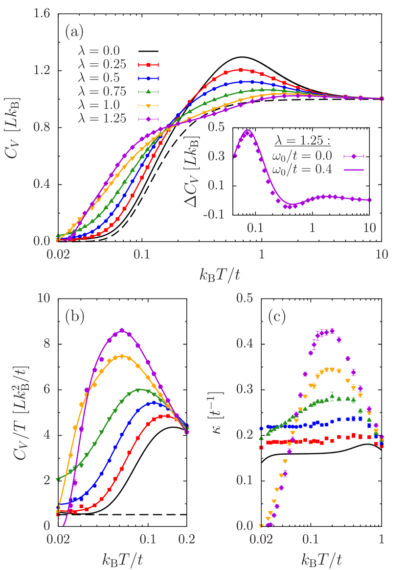
Figure 7: (a) Specific heat $C_{V}$, (b) specific heat over temperature $C_{V}/T$, and (c) compressibility $\kappa$ in the adiabatic regime ($\omega_{0}/t=0.4$, $L=162$). Data points correspond to direct estimates, whereas straight lines in (a) are obtained from fits to the total energy using the maximum entropy method. The dashed line in (a) corresponds to the free-phonon contribution, whereas the dashed line in (b) indicates the TLL result for $\lambda=0$. The inset in (a) shows $C_{V}$ for $\lambda=1.25$ minus the free-phonon contribution and compared to $\omega_{0}=0$.

Figure 7 shows the evolution of $C_{V}$ and $\kappa$ from weak to strong coupling at $\omega_{0}/t=0.4$. The specific heat in Fig. 7(a) exhibits a high-temperature electronic peak at $k_{\text{B}}T=\mathcal{O}(t)$ that is suppressed by the electron-phonon interaction, similar to $\omega_{0}=0$. However, quantum lattice fluctuations lead to a very different behavior at $k_{\text{B}}T\lesssim\omega_{0}$. Most notably, $C_{V}\to 0$ for $T\to 0$ as expected from the third law of thermodynamics.

To better contrast the low-temperature features of the metallic and insulating phases, we compare $C_{V}/T$ in Fig. 7(b) to $\kappa$ in Fig. 7(c). In contrast to the antiadiabatic regime, the low-energy phonon mode makes a substantial contribution to $C_{V}$ that only vanishes at the lowest temperatures considered. For $\lambda=0$, we can still identify the constant contribution to $C_{V}/T$ expected from Eq. (9) (dashed line, $u=v_{\text{F}}$) at low temperatures, although finite-size effects eventually become visible as $T\to 0$. For $\lambda>0$, the phonon softening around $q=\pi$ enhances $C_{V}$ at low $T$ and thereby complicates the analysis of the TLL behavior. From the maximum entropy fits to the total energy (solid lines), we deduce a reduction of the charge velocity with increasing $\lambda$ in accordance with Figs. 6(a) and (b). However, we cannot unambiguously determine $u$ from the QMC data because $C_{V}/T$ does not yet reach a plateau for the present temperatures and system size. By contrast, the compressibility in Fig. 7(c) does exhibit the expected constant behavior over a broad temperature range before finite-size effects set in. Even the small Peierls gap at $\lambda=0.75$ leads to a significant decrease of $\kappa$ at $k_{\text{B}}T/t<0.1$, whereas it does not leave any signature in $C_{V}/T$. Deep in the Peierls phase, for $\lambda=1.0$ and $\lambda=1.25$, $C_{V}/T,\kappa\to 0$ for $T\to 0$, as expected for a gapped system.

A comparison between Fig. 7(c) and Fig. 4(b) reveals that the temperature dependence of $\kappa$ in the Peierls phase is very similar to the classical case. For a direct comparison at $\lambda=1.25$, the inset of Fig. 7(a) shows $\Delta C_{V}$, corresponding to $C_{V}$ minus the temperature-dependent free-phonon contribution. Subtracting the free-phonon part appears justified since the phonon dispersion in Fig. 6(j) exhibits only minor renormalization effects compared to the noninteracting case. The comparison reveals good agreement between $\Delta C_{V}$ for $\omega_{0}/t=0.4$ and the adiabatic results, with minor differences only at intermediate temperatures. This suggests that deep in the Peierls phase the adiabatic approximation is valid and the opening of a pseudogap occurs at the same temperature scale as for $\omega_{0}=0$. The same holds for the electronic spectral function in Fig. 6(e) which qualitatively resembles the mean-field band structure. However, the gaps in Fig. 5(b) and Fig. 6(e) are smaller than $\Delta_{\text{MF}}$ (not shown).

IV.4 Crossover from low to high phonon frequencies

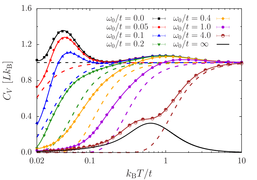
Figure 8: Specific heat $C_{V}$ for different $\omega_{0}$ at $\lambda=0.75$ and $L=162$. Dashed lines indicate the free-phonon contributions.

Finally, we exploit the unique advantages of our method to investigate the impact of quantum lattice fluctuations by calculating $C_{V}$ over the entire range of phonon frequencies from the adiabatic to the antiadiabatic limit at $\lambda=0.75$. Figure 8 reveals that the adiabatic approximation is valid for $k_{\text{B}}T\gtrsim\omega_{0}$. However, significant changes are visible at lower temperatures. For $\omega_{0}/t\lesssim 0.2$, we can approximate the phonon contribution by the noninteracting result (dashed lines), which drops to zero at a temperature scale that increases with increasing $\omega_{0}$. The low-temperature peak associated with pseudogap formation remains almost unchanged for $\omega_{0}/t\leq 0.1$. It can be identified even at $\omega_{0}/t=0.2$ after subtracting the free-phonon part (not shown). This suggests that the coherence temperature below which the 1D Peierls physics emerges remains almost unchanged for $\omega_{0}\ll\Delta_{\text{MF}}$. With increasing $\omega_{0}$, the formation of lattice defects in the dimerization pattern is accompanied by the creation of low-lying polaron states in $A(k,\omega)$ and a renormalization of the phonon dispersion in $B_{Q}(q,\omega)$ near $q=\pi$ (see Fig. 6). Eventually, both excitations become gapless at the critical value $\omega_{0,c}/t\gtrsim 0.4$ for the Peierls transition and leave a dominant low-temperature tail in $C_{V}$. For $\omega_{0}\gg\Delta_{\text{MF}}$ we recover separate electron and phonon contributions and $C_{V}$ approaches the result for noninteracting electrons as $\omega_{0}\to\infty$.

V Conclusions & Outlook

We studied the effects of quantum lattice fluctuations on the thermodynamic properties of Peierls chains using the paradigmatic spinless Holstein model. By means of a recently developed, highly efficient QMC method [46], we obtained accurate results for the specific heat over the entire range of model parameters. These results were complemented by calculations of the compressibility as well as electron and phonon spectral functions.

For classical phonons, the ground state is a Peierls insulator for any coupling. The specific heat exhibits a peak in the temperature range where dominant CDW correlations are suppressed and the Peierls gap is filled in. A second peak at higher temperatures is associated with the onset of coherence in the electronic spectrum. Deep in the Peierls phase, the effects of quantum lattice fluctuations are overall small and mostly restricted to the phonon contribution to $C_{V}$. On approaching the Peierls transition in the adiabatic regime, polaron excitations appear in the electronic spectrum and become gapless at the critical point. Moreover, in the adiabatic regime, the phonon spectrum exhibits a soft mode at the transition. Both types of low-energy excitations have a significant effect on $C_{V}$ at low temperatures. By contrast, in the nonadiabatic regime, electrons are strongly renormalized by polaronic effects even in the metallic phase. We were able to identify the expected, linear electronic contribution to $C_{V}$ proportional to the charge velocity. The renormalization of the latter was found to be particularly strong in the antiadiabatic regime, causing a shift of the electronic contribution to $C_{V}$ and hence the coherence scale to lower temperatures.

Regarding the thermodynamics of 1D Peierls systems, interesting open questions include the influence of the generic spin gap of the Luther-Emery phase and the interplay between electron-phonon and electron-electron interactions. Our exact 1D results provide the starting point for a systematic understanding of the experimental situation of quasi-1D materials in the framework of higher-dimensional models.

Appendix A Direct Monte Carlo estimator for the specific heat of the Holstein model

The SSE representation was originally formulated for instantaneous interactions, in which case it corresponds to a series expansion of the partition function in the total Hamiltonian. Therefore, the specific heat has the particularly simple estimator $C_{V}=\langle n^{2}\rangle-\langle n\rangle^{2}-\langle n\rangle$, corresponding to the fluctuations of the expansion order. To efficiently simulate fermion-boson models, we integrate over the bosonic fields and expand in terms of retarded interactions. As a result, we lose direct access to the bosonic fields and hence the Hamiltonian and can no longer use the above estimator for $C_{V}$. We have shown in Ref. [47] that the bosonic fields can be recovered from sum rules over fermionic correlation functions using generating functionals. Moreover, the total energy can be calculated efficiently from the distribution of vertices using the properties of the perturbation expansion [61]. In the following, we show that even the second moment of the Hamiltonian can be calculated in $\mathcal{O}(n)$ operations from the distribution of vertices. To set the notation, we begin with a brief discussion of the interaction vertex of the Holstein model. For completeness, we first outline the estimator for the total energy before turning to the estimator for the second moment of the Hamiltonian.

A.1 Interaction vertex of the Holstein model

The directed-loop algorithm for retarded interactions is based on the generic formulation of the perturbation expansion in the path-integral representation discussed in Ref. [47]. The Monte Carlo sampling is over configurations $C=\{n,C_{n},\ket{\alpha}\}$ defined by the expansion order $n$, the ordered vertex list $C_{n}=\{\nu_{1},\dots,\nu_{n}\}$, and the state $\ket{\alpha}$ in the local occupation number basis. In Ref. [46], we defined the interaction vertex for the spinless Holstein model. In the following, we extend it to the spinful case, where each subvertex $j\in\{1,2\}$ now has local variables $\{a_{j},b,\sigma_{j},\tau_{j}\}$ labeling its operator type, bond, spin, and imaginary time. The interaction vertex becomes

$$\mathcal{S}_{1}=-\iint_{0}^{\beta}d\tau_{1}d\tau_{2}\,P_{\!+}(\tau_{1}-\tau_{2})\sum_{\begin{subarray}{c}a_{1},a_{2},b,\\ \sigma_{1},\sigma_{2}\end{subarray}}h_{a_{1}a_{2},b}^{\sigma_{1}\sigma_{2}}(\tau_{1},\tau_{2})\,.$$ (11)

Here and in the following, we use the (anti-)symmetrized phonon propagators $P_{\!\pm}(\tau)=\frac{1}{2}\left[P(\tau)\pm P(\beta-\tau)\right]$ with $P(\tau)=\omega_{0}\exp(-\omega_{0}\tau)/[1-\exp(-\omega_{0}\beta)]$. The off-diagonal hopping vertices are given by

$$h_{10,b}^{\sigma_{1}\sigma_{2}}(\tau_{1},\tau_{2}) =\frac{t}{2N_{\sigma}}\,B_{b,\sigma_{1}}(\tau_{1})\,\mathbb{1}_{b,\sigma_{2}}(\tau_{2})\,,$$

$$h_{01,b}^{\sigma_{1}\sigma_{2}}(\tau_{1},\tau_{2}) =\frac{t}{2N_{\sigma}}\,\mathbb{1}_{b,\sigma_{1}}(\tau_{1})\,B_{b,\sigma_{2}}(\tau_{2})\,,$$ (12)

whereas the diagonal interaction vertices read

$$h_{22,b}^{\sigma_{1}\sigma_{2}}(\tau_{1},\tau_{2})=\lambda t\big{[}C +\rho_{i(b),\sigma_{1}}(\tau_{1})\,\rho_{i(b),\sigma_{2}}(\tau_{2})$$

$$+\rho_{j(b),\sigma_{1}}(\tau_{1})\,\rho_{j(b),\sigma_{2}}(\tau_{2})\big{]}$$ (13)

with $j(b)=i(b)+1$. We introduced an additional factor $N_{\sigma}$ in the hopping terms that counts the number of spin flavors and compensates the sum over the second spin index. For the spinful Holstein model, we have $N_{\sigma}=2$, whereas the spinless case is recovered by choosing $N_{\sigma}=1$ and dropping the spin indices. The constant shift $C$ in Eq. (13) ensures positive Monte Carlo weights. While we only consider the half-filled Holstein model, a chemical potential can be easily included in the diagonal term. In the following, we partition the total expansion order $n=n_{1}+n_{2}$ into the number of off-diagonal vertices $n_{1}=n_{10}+n_{01}$ and the number of diagonal vertices $n_{2}=n_{22}$.

A.2 Total energy

For completeness, we review the estimator for the total energy derived in Ref. [47]. The Hamiltonian of the Holstein model, $\hat{H}=\sum_{x}\hat{H}_{x}$, is split into three contributions labeled by the indices $x\in\{\text{el},\text{ph},\text{ep}\}$. The first element corresponds to the kinetic energy of the electrons, the second to the purely bosonic part (including a shift of $\omega_{0}/2$ per site), and the third to the electron-phonon interaction—see Eq. (1) for exact definitions. For each Monte Carlo configuration, we define the contributions to the total energy by

$$E_{x}(C_{n})=\frac{1}{\beta}\int_{0}^{\beta}d\tau\left\llangle H_{x}(\tau)\right\rrangle_{C_{n}}\,.$$ (14)

Translational invariance of all vertices is taken into account by the average over imaginary time. Using the sum rules specified in Ref. [47], each contribution to $E(C_{n})$ can be expressed in terms of the interaction vertices (12) and (13) to obtain

$$E_{\mathrm{el}}(C_{n}) =-\frac{n_{1}}{\beta}\,,$$ (15)

$$E_{\mathrm{ph}}(C_{n}) =L\,P_{\!+}(0)-{\lambda tCLN_{\sigma}^{2}}$$

$$\phantom{=}+\sum_{k=1}^{n_{2}}\left[\bar{P}_{\!+}(\tau_{k}-\tau^{\prime}_{k})-\bar{P}_{\!-}(\tau_{k}-\tau^{\prime}_{k})\right]\,,$$ (16)

$$E_{\mathrm{ep}}(C_{n}) =-\frac{2n_{2}}{\beta}+2\lambda tCLN_{\sigma}^{2}\,.$$ (17)

Translational invariance of all vertices is contained in the averaged propagator

$$\bar{P}_{\!\pm}(\tau_{k}-\tau^{\prime}_{k})=\frac{1}{\beta}\int_{0}^{\beta}d\tau\,\frac{P_{\!\pm}(\tau_{k}+\tau)P_{\!\pm}(\tau^{\prime}_{k}+\tau)}{P_{\!+}(\tau_{k}-\tau^{\prime}_{k})}\,.$$ (18)

Explicitly, it is given by ($\tau\in[-\beta,\beta]$)

$$\bar{P}_{\!\pm}(\tau)=\frac{1}{2\beta} \pm\frac{\omega_{0}}{4}\frac{\beta-\left|\tau\right|}{\beta}\left[\coth(\omega_{0}\beta/2)-\frac{P_{\!-}(\tau)}{P_{\!+}(\tau)}\right]$$

$$\pm\frac{\omega_{0}}{4}\frac{\left|\tau\right|}{\beta}\left[\coth(\omega_{0}\beta/2)+\frac{P_{\!-}(\tau)}{P_{\!+}(\tau)}\right]\,.$$ (19)

A.3 Second moment of the Hamiltonian

To calculate the second moment of $\hat{H}$, we write its expectation value in a translationally invariant form, i.e.,

$$\left\langle\hat{H}^{2}\right\rangle=\frac{1}{\beta^{2}}\iint_{0}^{\beta}d\tau d\tau^{\prime}\left\langle H(\tau)\,H(\tau^{\prime})\right\rangle\,.$$ (20)

Using the time-displaced form of the correlation function ensures that in the end each operator identified with a subvertex of the interaction vertex obtains an individual time label that is integrated over. We again split the total Hamiltonian into fermionic, bosonic, and fermion-boson contributions. To simplify the notation, we define ($x,x^{\prime}\in\{\text{el},\text{ph},\text{ep}\}$)

$$F_{x-x^{\prime}}(C_{n})=\frac{1}{\beta^{2}}\iint_{0}^{\beta}d\tau d\tau^{\prime}\left\llangle H_{x}(\tau)\,H_{x^{\prime}}(\tau^{\prime})\right\rrangle_{C_{n}}\,.$$ (21)

The estimator for the purely electronic contribution has the same form as usual and is given by

$$F_{\text{el}-\text{el}}(C_{n})=\frac{n_{1}\left(n_{1}-1\right)}{\beta^{2}}\,.$$ (22)

Also the mixing terms between the electronic part of the Hamiltonian and the remaining parts have simple estimators that are given by

$$F_{\text{el}-\text{ph}}(C_{n}) =E_{\mathrm{el}}(C_{n})\,E_{\mathrm{ph}}(C_{n})\,,$$ (23)

$$F_{\text{el}-\text{ep}}(C_{n}) =E_{\mathrm{el}}(C_{n})\,E_{\mathrm{ep}}(C_{n})\,.$$ (24)

The electronic and the bosonic contributions are recovered from vertices with different operator types and hence do not interfere in the total estimators.

The derivation of estimators is more complicated for correlation functions, where each part of the Hamiltonian contains bosonic fields. When we calculate the functional derivatives to obtain sum rules for the bosonic fields, we have to account for additional cross terms that do not appear for the individual energies. For example, the correlation function between the electron-phonon parts of the Hamiltonian becomes

$$\left\langle H_{\text{ep}}(\tau)\,H_{\text{ep}}(\tau^{\prime})\right\rangle=4 \lambda t\,P_{\!+}(\tau-\tau^{\prime})\sum_{i}\left\langle\rho_{i}(\tau)\rho_{i}(\tau^{\prime})\right\rangle$$

$$+(4\lambda t)^{2}\iint_{0}^{\beta}d\tau_{1} d\tau_{2}\,P_{\!+}(\tau-\tau_{1})\,P_{\!+}(\tau^{\prime}-\tau_{2})$$

$$\times\sum_{ij} \left\langle\rho_{i}(\tau)\rho_{i}(\tau_{1})\rho_{j}(\tau^{\prime})\rho_{j}(\tau_{2})\right\rangle\,.$$ (25)

The first term on the r.h.s. is an additional cross term. The corresponding estimator is

$$F_{\text{ep}-\text{ep}}(C_{n})=E_{\mathrm{ep}}(C_{n})^{2}-\frac{4n_{2}}{\beta^{2}}-\frac{E_{\mathrm{ep}}(C_{n})}{\beta}\,.$$ (26)

Similar considerations yield the estimators

$$F_{\text{ep}-\text{ph}}(C_{n})=E_{\mathrm{ep}}(C_{n})\,E_{\mathrm{ph}}(C_{n})+\frac{2\lambda tCLN_{\sigma}^{2}}{\beta}$$ (27)

and

$$F_{\text{ph}-\text{ph}}(C_{n}) =E_{\mathrm{ph}}(C_{n})^{2}+L\,P_{\!+}(0)\left[\bar{P}_{\!+}(0)-\bar{P}_{\!-}(0)\right]$$

$$\phantom{=\ }-\sum_{k=1}^{n_{2}}\left[\bar{P}_{\!+}(\tau_{k}-\tau^{\prime}_{k})-\bar{P}_{\!-}(\tau_{k}-\tau^{\prime}_{k})\right]^{2}$$

$$\phantom{=\ }+\sum_{k=1}^{n_{2}}\frac{Z(\tau_{k}-\tau^{\prime}_{k})}{P_{\!+}(\tau_{k}-\tau^{\prime}_{k})}-\frac{2\lambda tCLN_{\sigma}^{2}}{\beta}\,.$$ (28)

For the latter, we introduced an additional function

$$Z(\tau)=\frac{\omega_{0}^{3}}{\beta^{2}}\,e^{(\beta-\tau)\omega_{0}}\,n_{\text{B}}(\omega_{0})\,\big{[} \tau^{2}+\beta\left(\beta+2\tau\right)n_{\text{B}}(\omega_{0})$$

$$+2\beta^{2}n_{\text{B}}(\omega_{0})^{2}\big{]}$$ (29)

that is defined for $\tau\in[0,\beta)$. To evaluate $Z(\tau)$ for $\tau<0$, we use $Z(\tau+\beta)=Z(\tau)$. Here, $n_{\text{B}}(\omega)=[\exp(\beta\omega)-1]^{-1}$.

References

- Fröhlich [1954] H. Fröhlich, Proc. Roy. Soc. A 223, 296 (1954).
- Peierls [1955] R. E. Peierls, Quantum Theory of Solids (Clarendon Press, Oxford, 1955).
- Claessen et al. [2002] R. Claessen, M. Sing, U. Schwingenschlögl, P. Blaha, M. Dressel, and C. S. Jacobsen, Phys. Rev. Lett. 88, 096402 (2002).
- Travaglini et al. [1983] G. Travaglini, I. Mörke, and P. Wachter, Solid State Commun. 45, 289 (1983).
- Pytte [1974] E. Pytte, Phys. Rev. B 10, 4637 (1974).
- Hase et al. [1993] M. Hase, I. Terasaki, and K. Uchinokura, Phys. Rev. Lett. 70, 3651 (1993).
- Craven et al. [1974] R. A. Craven, M. B. Salamon, G. DePasquali, R. M. Herman, G. Stucky, and A. Schultz, Phys. Rev. Lett. 32, 769 (1974).
- Wei et al. [1977] T. Wei, A. J. Heeger, M. B. Salamon, and G. E. Delker, Solid State Commun. 21, 595 (1977).
- Biljakovic et al. [1986] K. Biljakovic, J. C. Lasjaunias, F. Zougmore, P. Monceau, F. Levy, L. Bernard, and R. Currat, Phys. Rev. Lett. 57, 1907 (1986).
- Liu et al. [1995] X. Liu, J. Wosnitza, H. von Löhneysen, and R. K. Kremer, Phys. Rev. Lett. 75, 771 (1995).
- Powell et al. [1998] D. K. Powell, J. W. Brill, Z. Zeng, and M. Greenblatt, Phys. Rev. B 58, R2937 (1998).
- Kwok et al. [1990] R. S. Kwok, G. Gruner, and S. E. Brown, Phys. Rev. Lett. 65, 365 (1990).
- Pouget [2016] J.-P. Pouget, Comptes Rendus Physique 17, 332 (2016).
- Ashcroft and Mermin [1976] N. W. Ashcroft and N. D. Mermin, Solid State Physics (Saunders College Publishing, Philadelphia, 1976).
- Kuiper [1955] C. G. Kuiper, Proc. Roy. Soc. A 227, 214 (1955).
- Heeger et al. [1988] A. J. Heeger, S. Kivelson, J. R. Schrieffer, and W. P. Su, Rev. Mod. Phys. 60, 781 (1988).
- Scalapino et al. [1972] D. J. Scalapino, M. Sears, and R. A. Ferrell, Phys. Rev. B 6, 3409 (1972).
- Lee et al. [1973] P. A. Lee, T. M. Rice, and P. W. Anderson, Phys. Rev. Lett. 31, 462 (1973).
- Weber et al. [2016a] M. Weber, F. F. Assaad, and M. Hohenadler, Phys. Rev. B 94, 155150 (2016a).
- Weiße and Fehske [1998] A. Weiße and H. Fehske, Phys. Rev. B 58, 13526 (1998).
- Wellein et al. [1998] G. Wellein, H. Fehske, and A. P. Kampf, Phys. Rev. Lett. 81, 3956 (1998).
- Hohenadler et al. [2006] M. Hohenadler, G. Wellein, A. R. Bishop, A. Alvermann, and H. Fehske, Phys. Rev. B 73, 245120 (2006).
- Fradkin and Hirsch [1983] E. Fradkin and J. E. Hirsch, Phys. Rev. B 27, 1680 (1983).
- Hirsch and Fradkin [1983] J. E. Hirsch and E. Fradkin, Phys. Rev. B 27, 4302 (1983).
- McKenzie et al. [1996] R. H. McKenzie, C. J. Hamer, and D. W. Murray, Phys. Rev. B 53, 9676 (1996).
- Kühne and Löw [1999] R. W. Kühne and U. Löw, Phys. Rev. B 60, 12125 (1999).
- Sandvik and Campbell [1999] A. W. Sandvik and D. K. Campbell, Phys. Rev. Lett. 83, 195 (1999).
- Hohenadler et al. [2011] M. Hohenadler, H. Fehske, and F. F. Assaad, Phys. Rev. B 83, 115105 (2011).
- Jeckelmann et al. [1999] E. Jeckelmann, C. Zhang, and S. R. White, Phys. Rev. B 60, 7950 (1999).
- Barford and Bursill [2005] W. Barford and R. J. Bursill, Phys. Rev. Lett. 95, 137207 (2005).
- Hager et al. [2007] G. Hager, A. Weiße, G. Wellein, E. Jeckelmann, and H. Fehske, J. Magn. Magn. Mater. 310, 1380 (2007).
- Ejima and Fehske [2009] S. Ejima and H. Fehske, Europhys. Lett. 87, 27001 (2009).
- Bursill et al. [1998] R. J. Bursill, R. H. McKenzie, and C. J. Hamer, Phys. Rev. Lett. 80, 5607 (1998).
- Caron and Bourbonnais [1984] L. G. Caron and C. Bourbonnais, Phys. Rev. B 29, 4230 (1984).
- Trebst et al. [2001] S. Trebst, N. Elstner, and H. Monien, Europhys. Lett. 56, 268 (2001).
- Sykora et al. [2005] S. Sykora, A. Hübsch, K. W. Becker, G. Wellein, and H. Fehske, Phys. Rev. B 71, 045112 (2005).
- Bühler et al. [2004] A. Bühler, G. S. Uhrig, and J. Oitmaa, Phys. Rev. B 70, 214429 (2004).
- Bakrim and Bourbonnais [2015] H. Bakrim and C. Bourbonnais, Phys. Rev. B 91, 085114 (2015).
- Braden et al. [1996] M. Braden, G. Wilkendorf, J. Lorenzana, M. Aïn, G. J. McIntyre, M. Behruzi, G. Heger, G. Dhalenne, and A. Revcolevschi, Phys. Rev. B 54, 1105 (1996).
- Feiguin and Fiete [2010] A. E. Feiguin and G. A. Fiete, Phys. Rev. B 81, 075108 (2010).
- Karrasch and Moore [2012] C. Karrasch and J. E. Moore, Phys. Rev. B 86, 155156 (2012).
- Hohenadler and Lang [2008] M. Hohenadler and T. C. Lang, in Computational Many-Particle Physics, edited by H. Fehske, R. Schneider, and A. Weiße (Springer Berlin Heidelberg, Berlin, Heidelberg, 2008) pp. 357–366.
- Fye and Scalettar [1987] R. M. Fye and R. T. Scalettar, Phys. Rev. B 36, 3833 (1987).
- Orignac and Chitra [2004] E. Orignac and R. Chitra, Phys. Rev. B 70, 214436 (2004).
- Voit and Schulz [1987] J. Voit and H. J. Schulz, Phys. Rev. B 36, 968 (1987).
- Weber et al. [2017] M. Weber, F. F. Assaad, and M. Hohenadler, Phys. Rev. Lett. 119, 097401 (2017).
- Weber et al. [2016b] M. Weber, F. F. Assaad, and M. Hohenadler, Phys. Rev. B 94, 245138 (2016b).
- Holstein [1959] T. Holstein, Ann. Phys. (N.Y.) 8, 325 (1959); 8, 343 (1959).
- Hohenadler and Fehske [2017] M. Hohenadler and H. Fehske, arXiv:1706.00470 (2017).
- Meden et al. [1994] V. Meden, K. Schönhammer, and O. Gunnarsson, Phys. Rev. B 50, 11179 (1994).
- Sykora et al. [2006] S. Sykora, A. Hübsch, and K. W. Becker, Europhys. Lett. 76, 644 (2006).
- Greitemann et al. [2015] J. Greitemann, S. Hesselmann, S. Wessel, F. F. Assaad, and M. Hohenadler, Phys. Rev. B 92, 245132 (2015).
- Weber et al. [2015a] M. Weber, F. F. Assaad, and M. Hohenadler, Phys. Rev. B 91, 245147 (2015a).
- Cross and Fisher [1979] M. C. Cross and D. S. Fisher, Phys. Rev. B 19, 402 (1979).
- Werner et al. [1999] R. Werner, C. Gros, and M. Braden, Phys. Rev. B 59, 14356 (1999).
- Zimanyi et al. [1988] G. T. Zimanyi, S. A. Kivelson, and A. Luther, Phys. Rev. Lett. 60, 2089 (1988).
- Feynman [1955] R. P. Feynman, Phys. Rev. 97, 660 (1955).
- Sandvik and Kurkijärvi [1991] A. W. Sandvik and J. Kurkijärvi, Phys. Rev. B 43, 5950 (1991).
- Syljuasen and Sandvik [2002] O. Syljuasen and A. W. Sandvik, Phys. Rev. E 66, 046701 (2002).
- Sandvik [1992] A. W. Sandvik, J. Phys. A: Math. Gen. 25, 3667 (1992).
- Sandvik et al. [1997] A. W. Sandvik, R. R. P. Singh, and D. K. Campbell, Phys. Rev. B 56, 14510 (1997).
- Huscroft et al. [2000] C. Huscroft, R. Gass, and M. Jarrell, Phys. Rev. B 61, 9300 (2000).
- Jarrell and Gubernatis [1996] M. Jarrell and J. E. Gubernatis, Phys. Rep. 269, 133 (1996).
- Dorneich and Troyer [2001] A. Dorneich and M. Troyer, Phys. Rev. E 64, 066701 (2001).
- Weber et al. [2015b] M. Weber, F. F. Assaad, and M. Hohenadler, Phys. Rev. B 91, 235150 (2015b).
- Sandvik [1998] A. W. Sandvik, Phys. Rev. B 57, 10287 (1998).
- Beach [2004] K. S. D. Beach, arXiv:cond-mat/0403055 (2004).
- Kadanoff and Baym [1989] L. P. Kadanoff and G. A. Baym, Quantum Statistical Mechanics: Green’s Function Methods in Equilibrium and Nonequilibrium Problems (Addison-Wesley, Redwood City, California, 1989).
- Schneider and Wierstorf [2014] A. Schneider and H. Wierstorf, “Gnuplot-colorbrewer: ColorBrewer color schemes for gnuplot,” 10.5281/zenodo.10282 (2014).
- Lang and Firsov [1962] I. G. Lang and Y. A. Firsov, Zh. Eksp. Teor. Fiz. 43, 1843 (1962), [Sov. Phys. JETP 16, 1301 (1962)].
- Loos et al. [2006] J. Loos, M. Hohenadler, and H. Fehske, J. Phys.: Condens. Matter 18, 2453 (2006).
- Giamarchi [2004] T. Giamarchi, Quantum physics in one dimension, Internat. Ser. Mono. Phys. (Clarendon Press, Oxford, 2004).
- Voit et al. [2000] J. Voit, L. Perfetti, F. Zwick, H. Berger, G. Margaritondo, G. Grüner, H. Höchst, and M. Grioni, Science 290, 501 (2000).
- Michielsen and de Raedt [1996] K. Michielsen and H. de Raedt, Mod. Phys. Lett. B 10, 467 (1996).
- Michel and Evertz [2007] F. Michel and H. G. Evertz, arXiv:0705.0799 (2007).
- Assaad and Evertz [2008] F. F. Assaad and H. G. Evertz, in Computational Many-Particle Physics, edited by H. Fehske, R. Schneider, and A. Weiße (Springer Berlin Heidelberg, Berlin, Heidelberg, 2008) pp. 277–356.
- Jülich Supercomputing Centre [2016] Jülich Supercomputing Centre, J. Large-Scale Res. Facilities 2, A62 (2016).