Sparse Low Rank Approximation of Potential Energy Surfaces with Applications in Estimation of Anharmonic Zero Point Energies and Frequencies

Abstract

We propose a method that exploits sparse representation of potential energy surfaces (PES) on a polynomial basis set selected by compressed sensing. The method is useful for studies involving large numbers of PES evaluations, such as the search for local minima, transition states, or integration. We apply this method for estimating zero point energies and frequencies of molecules using a three step approach. In the first step, we interpret the PES as a sparse tensor on polynomial basis and determine its entries by a compressed sensing based algorithm using only a few PES evaluations. Then, we implement a rank reduction strategy to compress this tensor in a suitable low-rank canonical tensor format using standard tensor compression tools. This allows representing a high dimensional PES as a small sum of products of one dimensional functions. Finally, a low dimensional Gauss-Hermite quadrature rule is used to integrate the product of sparse canonical low-rank representation of PES and Green’s function in the second-order diagrammatic vibrational many-body Green’s function theory (XVH2) for estimation of zero-point energies and frequencies. Numerical tests on molecules considered in this work suggest a more efficient scaling of computational cost with molecular size as compared to other methods.

1 Introduction

Electronic structure calculations have been developed as a powerful tool that is used in several fields including chemical sciences and biochemistry, as well as material and energy sciences. In ab initio electronic structure calculations, for instance, computation (and often storage) of six-dimensional integrals involving two-body (i.e., Coulomb) interactions (“two-electron integrals") is necessary, creating a severe bottleneck of such calculations for larger molecules [1]. In quantum dynamics, accurate estimation of energy and vibrational frequencies of molecules requires integration of functions whose dimensionality increases linearly with $a$, the number of nuclei in the molecule. For example, the potential energy surfaces (PESs) are often a part of the integrand, and their dimensionality increases as $(3a-6)$, where $a$ is the number of atoms. Thus efficient ways to approximate and integrate high dimensional PESs that exploit their special structure, if it exists, are needed.

Numerical approximation or integration of these PESs, in practice, can be carried out via sampling techniques with the function as a black-box. For example, one probes the PES at different configuration of atoms in a molecule with standard quantum chemistry software packages such as NWChem [2]. Many methods to represent a PES using a set of energy data points exist. Some of the black-box fitting methods include splines [3, 4], modified-Shepard interpolation [5], interpolating moving least squares [6, 7], neural networks [8, 9, 10, 11, 12, 13], and reproducing kernel Hilbert space [14]. These methods, although efficient with PES approximation of smaller systems, do not usually scale well with system size and may suffer with severe computational constraints. Also, the functional form of the approximation may not render it in a way that is easy to integrate or employ further in a given computational pipeline.

Methods for accurate PES approximation of bigger molecules with relatively few PES evaluations are needed. Mathematically, for high dimensional functions, application of standard approximation approaches is often not sufficient due to the curse of dimensionality, i.e. when the required computational effort increases exponentially with dimension. One usually employs a class of methods that exploit specific structures of high dimensional functions, such as smoothness or sparsity (see chapter 1 of [15] for a brief survey). In this work, we first exploit the sparsity property of the PES using compressed sensing [16, 17] methods from the signal processing community. The mathematical theory of compressed sensing is well-developed and is being used in many scientific applications. Some of the experimental applications of compressed sensing include multidimensional nuclear magnetic resonance [18, 19], super-resolution microscopy [20] and other applications in spectroscopy and beyond [21, 22, 23, 24, 25]. Compressed sensing is also becoming a method of choice for computational applications [26, 27, 28, 29]. For example, in [30], compressed sensing is used to reduce the amount of computation in numerical simulations for molecular vibrations.

Sparse approximation using compressed sensing relies on the fact that a good approximation of the PES can be obtained by representing it as a linear combination of only a few basis functions chosen from a well-constructed set of basis functions [31, 32]. Existence of sparsity structure can be attributed to the fact that the function is not equally coupled in all dimensions and hence only a few basis functions are important for an accurate representation. Here, the basis set consists of tensor products of orthogonal polynomials, and its subset is obtained with a constraint imposed on the total order of these multivariate polynomials. The approximation obtained can then be interpreted as a sparse tensor. We then exploit the low rank structure [33, 34, 35] in a subsequent step by applying a rank reduction strategy on the sparse tensor. Here, a high rank representation of a PES is compressed as a small sum of products of low dimensional functions [36, 37]. Finally, these low dimensional integrals are integrated using a Gauss-Hermite quadrature rule. The proposed approach thus presents a synthesis of three ideas: sparse approximation, low rank compression and quadrature for the estimation of zero point energies and frequencies in XVH2. This approach is efficient, and has a strong potential for scalability with molecular size. Note that methods that explicitly make use of low rank structure of the PES have recently been proposed [38, 39].

The outline of the paper is as follows. In Section 2, we discuss the tensor interpretation of functions and its approximation using least-squares with sparse regularization via compressed sensing. Then, in Section 3, we present a general method for compressing functions represented on a tensor product basis and apply it for integrating high dimensional functions using separated integration. In Section 4, we recall formulations in quantum chemistry that lead to first and second order corrections to the zero point energy and anharmonic molecular vibrations. In Section 5, we illustrate the application of the proposed method on four different molecules with increasing dimensionality of PES. Finally, we conclude with perspectives in Section 6.

2 Sparse Approximation of Potential Energy Surfaces

Very often in scientific discovery and applications, one may collect a large amount of data but only a subset of it may be relevant to study the problem at hand. The difficulty however is that one does not know a priori where the useful information can be found and how much information is sufficient. In approximation of PES of a system, one is required to evaluate the surface as many times as the underlying model assumption or the numerical scheme needs to provide a closed form solution. For example, consider the the representation of PES as a multivariate function $u(\bm{x})$ expanded on a multidimensional tensor product basis as

$$u(\bm{x})\approx\tilde{u}(\bm{x})=\sum_{j_{1}=0}^{p_{1}}\cdots\sum_{j_{m}=0}^{p_{m}}v_{j_{1},\ldots,j_{m}}\phi^{(1)}_{j_{1}}(x_{1})\cdots\phi^{(m)}_{j_{m}}(x_{m}),$$ (1)

where $\phi^{(i)}_{j_{i}}(x_{i})$ is the $j_{i}$th basis function in the $i$th coordinate, $x_{i}$. Here, the total number of coefficients of the multidimensional basis needed to characterize $\tilde{u}(\bm{x})$ is given by $P=\prod_{k=1}^{m}p_{k}$. For the sake of simplicity, let us choose the same number of basis functions, $p$, in each dimension such that $P=p^{m}$. For a high dimensional PES, $m$ is large, and the exponential increase in bases terms is referred to as the curse of dimensionality. For example, a least squares based approximation of $u(\bm{x})$ will require at least $P$ evaluations of $u(\bm{x})$ which, in general, may not be feasible. However, if we are only interested in an accurate estimate of integration of $u(\bm{x})$ over a domain $\Omega$, as in this work (and not, for example, in point-wise accuracy of the surface), then we can drastically reduce the number of required evaluations of $u(\bm{x})$.

The mathematical assumption that enables a good approximation with only a few evaluations of $u(\bm{x})$ is that of all coefficients $v_{j_{1},\ldots,j_{m}}$ in (1) only a few are nonzero. Under this assumption, $u(\bm{x})$ is said to be sparse on multidimensional bases $\phi^{(1)}_{j_{1}}(x_{1})\cdots\phi^{(m)}_{j_{m}}(x_{m})$. The problem then reduces to finding the nonzero coefficients such that the number of evaluations of $u(\bm{x})$ required is proportional to only the number of nonzero coefficients. In order to achieve this objective, we use a two-fold approach. First, we choose $\phi^{(i)}_{j_{i}}(x_{i})$ as orthogonal polynomials and a priori reduce the number of multidimensional bases in (1) based on their total degree (to be defined below). Second, we further take advantage of sparsity of $u(\bm{x})$ in its representation in the reduced basis set by using techniques from compressed sensing. Both approaches are detailed in the following subsections.

2.1 A priori reduction of basis set

In this section, we propose an a priori reduction of the tensor product basis set for the representation of potential energy functions under the assumption that they admit limited degree of high-order interactions. It is well known that, for smooth functions, polynomials are a natural choice of basis functions for functional representation. Let us denote the set of multidimensional polynomials with degree per-dimension $p$ as

$$\mathbb{Q}_{p}=\left\{\prod_{i=1}^{m}\phi^{(i)}_{j_{i}}(x_{i}):\mathbf{j}\in\mathbb{N}_{0}^{m},|\mathbf{j}|_{\infty}:=\underset{i\in\{1\ldots m\}}{\mathrm{max}}j_{i}\leq p\right\},$$ (2)

where $\phi^{(i)}_{j_{i}}(x_{i})$ is a polynomial of degree $j_{i}$ and $\mathbf{j}$ is a multi-index $(j_{1},\ldots,j_{m})$ in the set of multi-indices $\mathcal{J}=\times_{i=1}^{m}\{0,\ldots,p\}$. The total number of basis functions for a given $p$ in this set is given by $(p+1)^{m}$. For example, in (1), $u(\bm{x})$ is represented on the basis in $\mathbb{Q}_{p}$ when $p_{1}=\ldots=p_{m}=p$. Another alternative is the set of multidimensional polynomials of total degree $p$ defined by:

$$\mathbb{P}_{p}=\left\{\prod_{i=1}^{m}\phi^{(i)}_{j_{i}}(x_{i}):\mathbf{j}\in\mathbb{N}_{0}^{m},|\mathbf{j}|_{1}:=\sum_{i=1}^{m}j_{i}\leq p\right\}.$$ (3)

Here the total number of basis functions for a given $p$ is given by $P=\frac{(m+p)!}{m!p!}$.

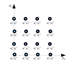
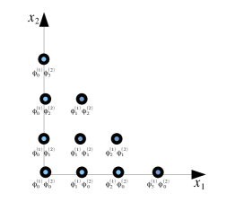
Figure 1: Illustration of basis functions in $\mathbb{Q}_{p}$ (left) and $\mathbb{P}_{p}$ (right) for degree $p=3$ and dimension $m=2$. The number of basis function in $\mathbb{Q}_{p}$ is $(3+1)^{2}=16$ whereas in $\mathbb{P}_{p}$ is $\frac{(3+2)!}{3!2!}=10.$

In Figure 1, we illustrate the set of basis functions in $\mathbb{Q}_{p}$ and $\mathbb{P}_{p}$ for $p=3$ and $m=2$. It can be clearly seen that $\mathbb{P}_{p}$ is a subset of $\mathbb{Q}_{p}$, albeit the number of elements in $\mathbb{P}_{p}$ still grows fast with dimension. The first step in this work is to reduce the number of basis functions for representation of $u(\bm{x})$ by choosing a priori the basis set $\mathbb{P}_{p}$ (and not $\mathbb{Q}_{p}$). Thus we are explicitly choosing the coefficients corresponding to those basis function in $\mathbb{Q}_{p}$ as zero that are not present in ${\mathbb{P}_{p}(\mathcal{X})}$. We can thus write the approximation of $u(\bm{x})$ as

$$u(\bm{x})\approx\tilde{u}(\bm{x})=\sum_{\mathbf{j}\in\tilde{\mathcal{J}}}v_{\mathbf{j}}\phi_{\mathbf{j}}(\bm{x}),$$ (4)

where $\mathbf{j}\in\tilde{\mathcal{J}}$ such that $|\mathbf{j}|_{1}\leq p$ and $v_{\mathbf{j}}$ is real coefficient on the basis $\phi_{\mathbf{j}}=\prod_{i=1}^{m}\phi_{j_{i}}^{(i)}$. In the next step, we further reduce the number of basis functions with non-zero coefficients in (4) using methods based on compressed sensing.

2.2 Sparse approximation using Compressed Sensing

Let us represent Eq. (4) as a linear system of equations

$${\boldsymbol{\Phi}}\mathbf{v}=\mathbf{u},$$ (5)

where $\mathbf{u}\in\mathbb{R}^{S}$ is a vector of $S$ evaluations of $u(\bm{x})$ on $\mathbf{x}^{s},s=1,\ldots,S$ realizations of $\bm{x}$ and ${\boldsymbol{\Phi}}\in\mathbb{R}^{S\times P}$ is the matrix whose row elements are basis functions $\phi_{\mathbf{j}}$ evaluated at $\mathbf{x}^{s}$ i.e. ${\boldsymbol{\Phi}}_{s\ell}=\phi_{{\mathbf{j}}_{\ell}}(\mathbf{x}^{s})$, where $\ell=1,\ldots,P$ indexes an ordering of $\mathbf{j}_{\ell}\in\tilde{\mathcal{J}}$. One can obtain the vector of coefficients $\mathbf{v}\in\mathbb{R}^{P}$ using least squares by

$$\mathbf{v}=({\boldsymbol{\Phi}}^{T}{\boldsymbol{\Phi}})^{-1}{\boldsymbol{\Phi}}^{T}\mathbf{u},$$ (6)

where, for a well-defined matrix inversion, one needs at least as many independent evaluations of $u(\bm{x})$ as the number of basis functions i.e. $S\geq P$. In the absence of sufficient number of evaluations i.e. $S<P$, (5) is an underdetermined system with an infinite number of solutions. However, if it is known that $\mathbf{v}$ is sparse, meaning that it has very few nonzero components, we can obtain a good approximation of $\mathbf{v}$ with $S\ll P$ using compressed sensing. Equivalently, compressed sensing endeavors to find a sufficiently accurate representation of $u(\bm{x})$ by only considering a finite subset of basis functions:

$$u(\bm{x})\approx\tilde{u}_{n}(\bm{x})=\sum_{\mathbf{j}\in\tilde{\mathcal{J}}_{n}}v_{\mathbf{j}}\phi_{\mathbf{j}}(\bm{x}).$$ (7)

Here $\tilde{\mathcal{J}}_{n}\subset\tilde{\mathcal{J}}$ such that $\tilde{u}_{n}(\bm{x})$ is represented on only $n\ll P$ basis functions. The $n$ nonzero components of $\mathbf{v}$ are obtained by formulating the following optimization problem

$$\underset{\|\mathbf{v}\|_{0}=n}{\mathrm{min}}\|{\boldsymbol{\Phi}}\mathbf{v}-\mathbf{u}\|_{2}^{2},$$ (8)

where $\|\cdot\|_{0}$ is the zero-norm of a vector and simply counts the number of nonzero components. The above problem is non-convex and we instead solve

$$\mathrm{min}\;\|{\boldsymbol{\Phi}}\mathbf{v}-\mathbf{u}\|_{2}^{2}+\lambda\|\mathbf{v}\|_{1},$$ (9)

where $\|\cdot\|_{1}$ is the $\ell_{1}$ norm i.e. sum of absolute values of components of a vector and $\lambda$ is a regularization coefficient. Problem (9) is a convex optimization problem for which several methods are available [40]. If $u(\bm{x})$ admits an accurate sparse approximation, then, under some additional conditions, solving (9) gives a sparse solution $\mathbf{v}$. This is the basis of the compressed sensing approach that made a breakthrough in signal processing more than a decade ago [16, 17, 41]. In this work, we use a Bayesian Compressed Sensing [42] algorithm, which has is implemented in the UQTk software [43], for approximately solving (9). We illustrate the application of compressed sensing in Figure 2 where we (symbolically) retain only a few basis functions from the set basis set $\mathbb{P}_{3}$ with nonzero coefficients in the sparse approximation of $u(\bm{x})$.

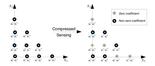
Figure 2: Illustration of application of compressed sensing based selection of basis functions with nonzero coefficients (right) from the basis set $\mathbb{P}_{2}$ (left).

Thus by combining the two methods explained in this section, we can greatly reduce the computational expense required to estimate a good approximation of $u(\bm{x})$. In high dimensions however, the number of retained basis functions $n$ can still be large and, depending on the application (ex. integration), one may be interested in a more compact representation of $\tilde{u}_{n}(\bm{x})$. In the following section, we detail our approach for integrating a compressed version of $\tilde{u}_{n}(\bm{x})$ using separated integration.

3 Separated Integration of Sparse Approximation

Let us consider the following integration problem

$$I[u]=\int\limits_{-\infty}^{+\infty}u(\bm{x})\rho(\bm{x})\mathrm{d}\bm{x},$$ (10)

where $\rho(\bm{x})$ is a non-negative weight function that is integrable and multiplicatively separable, i.e.,

$$\rho(\bm{x}) \geq 0,$$ (11)

$$\int\limits_{-\infty}^{+\infty}\rho(\bm{x})\mathrm{d}\bm{x} < \infty,$$ (12)

and

$$\rho(\bm{x}) = \prod_{i=1}^{m}\rho^{(i)}(x_{i}).$$ (13)

An approximation of (10) can be written as

$$I[u]\approx I[\tilde{u}_{n}]=\int\limits_{-\infty}^{+\infty}\tilde{u}_{n}(\bm{x})\rho(\bm{x})\mathrm{d}\bm{x}.$$ (14)

Substituting the sparse approximation of $\tilde{u}_{n}(\bm{x})$ from (7) into (14), we get

$$I[\tilde{u}_{n}]=\sum_{\mathbf{j}\in\tilde{\mathcal{J}}_{n}}v_{\mathbf{j}}\left(\prod_{i=1}^{m}\int\limits_{-\infty}^{+\infty}\phi^{(i)}_{j_{i}}\rho^{(i)}(x_{i})dx_{i}\right),$$ (15)

where the integrands in (15) are one dimensional polynomial functions and can be easily evaluated using standard quadrature rules. However, as will be seen in the second order corrections in XVH2 in Section 4.1, even if $n$ is only moderately large, the number of quadrature integrations required can increase rapidly. In order to improve computation efficiency, we can reduce the number of separated terms in $u_{n}(\bm{x})$, i.e. separation rank, considerably for a small loss of accuracy. We thus strive to find approximations of the form

$$\tilde{u}_{n}(\bm{x})\approx\tilde{u}_{r}(\bm{x})=\sum_{k=1}^{r\ll n}\alpha_{k}w_{k}(\bm{x}),\;\alpha_{k}\in\mathbb{R},$$ (16)

where

$$w_{k}(\bm{x})=\prod_{i=1}^{m}w^{(i)}_{k}(x_{i}),\>\textrm{ and }\>w^{(i)}_{k}(x_{i})=\sum_{j=1}^{p}w^{(i)}_{k,j}\phi_{j}^{(i)}(x_{i})$$ (17)

and $r$ is the separation rank. The univariate functions $w_{k}^{(i)}(x_{i})$, characterized by coefficient vectors $\mathbf{w}^{(i)}_{k}=(w^{(i)}_{k,1},\ldots,w^{(i)}_{k,p})$, are represented as expansions on bases ${\boldsymbol{\phi}}^{(i)}=(\phi_{1}^{(i)}(x_{i}),\ldots,\phi_{p}^{(i)}(x_{i}))$. Note that $\mathbf{w}^{(i)}_{k}$ and hence $w_{k}^{(i)}(x_{i})$ need not be sparse. Finding low rank approximations of the form (16) thus reduces to finding coefficient vectors $\mathbf{w}^{(i)}_{k},\;1\leq i\leq m,1\leq k\leq r$. The scalar coefficient $\alpha_{k}$ is obtained by normalizing $\mathbf{w}_{k}^{(i)},1\leq i\leq m$ such that $\|\mathbf{w}_{k}^{(i)}\|$ = 1. With this rank reduction procedure, we can greatly reduce the number of terms in the separated representation of the integrand thus reducing the computation time for quadrature based evaluation of the integrals i.e.

$$I[\tilde{u}_{n}]\approx I[\tilde{u}_{r}]=\sum_{k=1}^{r}\alpha_{k}\left(\prod_{i=1}^{m}\int\limits_{-\infty}^{+\infty}w^{(i)}_{k}(x_{i})\rho^{(i)}(x_{i})dx_{i}\right).$$ (18)

In Figure 3, we illustrate the rank reduction procedure designated by (16). Let us denote an $m^{th}$ order tensor $\tilde{\boldsymbol{\mathsf{U}}}_{n}$ whose entries are coefficients $v_{\mathbf{j}},\;\mathbf{j}\in\tilde{\mathcal{J}}_{n}$ in the sparse approximation given by (7). With choice of bases $\phi_{j}^{(i)},1\leq i\leq m,1\leq j\leq p$, function $\tilde{u}_{n}(\bm{x})$ can be identified with tensor $\tilde{\boldsymbol{\mathsf{U}}}_{n}$. Finding the low rank approximation $\tilde{u}_{r}(\bm{x})$ in (16) then reduces to finding a low rank decomposition of the tensor $\tilde{\boldsymbol{\mathsf{U}}}_{n}\approx\tilde{\boldsymbol{\mathsf{U}}}_{r}$ such that

$$\tilde{\boldsymbol{\mathsf{U}}}_{r}=\sum_{k=1}^{r}\alpha_{k}\left(\otimes_{i=1}^{m}\mathbf{w}_{k}^{(i)}\right).$$ (19)

The decomposition of the tensor in (19) is known as the canonical polyadic decomposition for which several tensor decomposition tools are available. In this work, we use the Tensor Toolbox[44].

Figure 3: Illustration of low rank decomposition of tensor $\tilde{\boldsymbol{\mathsf{U}}}_{r}$

We now wish to integrate the low rank function $u_{r}(\bm{x})$ with respect to a separable measure $\rho(\bm{x})$ via quadrature as

$$I[\tilde{u}_{r}]=\sum_{k=1}^{r}\alpha_{k}\left(\prod_{i=1}^{m}\int_{-\infty}^{+\infty}w^{(i)}_{k}(x_{i})\rho^{(i)}(x_{i})dx_{i}\right),$$ (20)

Let us denote $\gamma_{q_{i}}^{(i)}$ and $\mathrm{x}_{i}^{q_{i}},1\leq q_{i}\leq Q_{i}$ as one dimensional quadrature weights and quadrature points along dimension $i$ for the measure $\rho^{(i)}(x_{i})$. We can evaluate (20) as

$$I[u_{r}]=\sum_{k=1}^{r}\alpha_{k}\left(\prod_{i=1}^{m}\sum_{q_{i}=1}^{Q_{i}}\gamma^{(i)}_{q_{i}}w_{k}^{(i)}(\mathrm{x}_{i}^{q_{i}})\right).$$ (21)

Thus we integrate our function using $rm$ one dimensional integrals each of which is evaluated using quadrature at a total computational cost of $O(rmp)$, where $p$ is the degree of univariate polynomial functions $w_{k}^{(i)}(x_{i})$, increasing only linearly with dimension.

4 Integrals in XVH2

In this section, we motivate the utility of sparse low rank tensor based approximation of PES to find energy corrections and anharmonic frequencies of molecular vibrations.

4.1 First and second order energy corrections

Below, we list integrals in the second-order diagrammatic vibrational many-body Green’s function formalism. The reader is referred to the original papers [45, 46] for the derivations of this formalism and [38] for a detailed presentation of the following integrals.

In the following, we denote first and second order corrections to energy by $E^{(1)}_{0}$ and $E^{(2)}_{0}$ respectively. The anharmonic vibrational frequency of the $i$th mode ($\nu_{i}$) including up to the second-order perturbation correction can be obtained by frequency-independent, diagonal approximation to the Dyson equation [45]

$$\nu_{i}=\left\{\omega_{i}^{2}+2\omega_{i}\Sigma_{i}(0)\right\}^{1/2},$$ (22)

with

$$\Sigma_{i}(\nu) = \Sigma_{i}^{(1)}(\nu)+\Sigma_{i}^{\mathrm{(2p)}}(\nu)+\Sigma_{i}^{\mathrm{(2p^{\prime})}}(\nu)+$$ (23)

$$+\;\Sigma_{i}^{\mathrm{(2b)}}(\nu)+\Sigma_{i}^{\mathrm{(2b^{\prime})}}(\nu).$$

where $\omega_{i}$ is the $i$th harmonic frequency. Note that, in this work, we solve the Dyson equation non-self-consistently, i.e., we substitute $\nu=0$ in the right-hand sides of (22) and (23). Given these notations, our interest is in computing the integrals $E_{0}^{(1)},E_{0}^{(2)},\Sigma_{i}^{(1)}(0),\Sigma_{i}^{\mathrm{(2p)}}(0),$ $\Sigma_{i}^{\mathrm{(2p^{\prime})}}(0),\Sigma_{i}^{\mathrm{(2b)}}(0)$ and $\Sigma_{i}^{\mathrm{(2b^{\prime})}}(0)$.

We classify all integrals that appear in the formalisms of XVH2 into two groups. The first group consists of $m$-dimensional integrals ($m=3a-6$, where $a$ is the number of atoms in the non linear molecule), which are collectively written as

$$I^{(1)}=\int_{-\infty}^{+\infty}e(\bm{x})P^{(1)}(\bm{x})\mathrm{d}\bm{x}$$ (24)

with

$$e(\bm{x}) = \prod_{i=1}^{m}e^{-\omega_{i}x_{i}^{2}},$$ (25)

$$P^{(1)}(\bm{x}) = \Delta V(\bm{x})\prod_{i=1}^{m}\lambda_{i}^{(1)}(x_{i}),$$ (26)

where $\bm{x}=\{x_{1},\dots,x_{m}\}$ is the $m$-dimensional set of normal coordinates and $\lambda_{i}^{(1)}(x)$ is given in Table 1 for each case of $I^{(1)}=E_{0}^{(1)}$ or $I^{(1)}=\Sigma_{i}^{(1)}(0)$.

Table 1: The value of $\lambda_{i}^{(1)}(x_{i})$ in Equation (26).

$I^{(1)}$	$\lambda_{i}^{(1)}(x_{i})$
$E_{0}^{(1)}$	1
$\Sigma_{i}^{(1)}(0)$	${2^{1/2}\eta_{2}(x_{i})}/{\eta_{0}(x_{i})}$
$\Sigma_{j\neq i}^{(1)}(0)$	1

Here $\eta_{n_{i}}(x_{i})$ is the harmonic-oscillator wave function along the $i$th normal coordinate $x_{i}$ with quantum number $n_{i}$, namely,

$$\eta_{n_{i}}(x_{i})=N_{n_{i}}e^{-{\omega_{i}x_{i}^{2}}/{2}}h_{n_{i}}(\omega_{i}^{1/2}x_{i}).$$ (27)

Here, $N_{n_{i}}$ is the normalization coefficient, $h_{n_{i}}$ is the Hermite polynomial of degree $n_{i}$.

The fluctuation potential $\Delta V(\bm{x})$ is given by

$$\Delta V(\bm{x})=V(\bm{x})-V_{\mathrm{ref}}-\frac{1}{2}\sum_{i=1}^{m}\omega_{i}^{2}x_{i}^{2},$$ (28)

where $V(\bm{x})$ is the $m$-dimensional PES and $V_{\mathrm{ref}}$ is its value at the equilibrium geometry, which is the electronic energy at the equilibrium geometry of the molecule.

The second group involves $2m$-dimensional integrals of the form,

$$I^{(2)}=\int\limits_{-\infty}^{+\infty}\int\limits_{-\infty}^{+\infty}e(\bm{x},\bm{x}^{\prime})P^{(2)}(\bm{x},\bm{x}^{\prime})\mathrm{d}\bm{x}\mathrm{d}\bm{x}^{\prime}$$ (29)

with

$$e(\bm{x},\bm{x}^{\prime}) = \prod_{i=1}^{m}e^{-\omega_{i}(x_{i}^{2}+x^{\prime 2}_{i})},$$ (30)

$$P^{(2)}(\bm{x},\bm{x}^{\prime}) = \Delta V(\bm{x})\Delta V(\bm{x}^{\prime})G(\bm{x},\bm{x}^{\prime})\prod_{i=1}^{m}\lambda_{i}^{(2)}(x_{i},x_{i}^{\prime}),$$ (31)

where $G(\bm{x},\bm{x}^{\prime})$ is a real-space Green’s function given by

$$G(\bm{x},\bm{x}^{\prime})=\underset{(n_{1},n_{2},\dots,n_{m})\neq(0,0,\dots,0)}{\sum_{n_{1}=0}^{n_{\mathrm{max}}}\cdots\sum_{n_{m}=0}^{n_{\mathrm{max}}}}\prod_{i=1}^{m}\frac{N^{2}_{n_{i}}h_{n_{i}}(\omega_{i}^{1/2}x_{i})h_{n_{i}}(\omega_{i}^{1/2}x^{\prime}_{i})}{-\sum_{i=1}^{m}n_{i}\omega_{i}}.$$ (32)

Table 2 defines $\lambda_{i}^{(2)}(x_{i},x^{\prime}_{i})$ for each case under consideration.

Table 2: The value of $\lambda_{i}^{(2)}(x_{i},x^{\prime}_{i})$ in Equation (32).

$I^{(2)}$	$\lambda_{i}^{(2)}(x_{i},x^{\prime}_{i})$
$E_{0}^{(2)}$	1
$\Sigma_{i}^{\mathrm{(2p)}}(0)$	${(n_{i}+2)^{1/2}(n_{i}+1)^{1/2}\eta_{n_{i}+2}(x_{i}^{\prime})}/{\eta_{n_{i}}(x_{i}^{\prime})}$
$\Sigma_{j\neq i}^{\mathrm{(2p)}}(0)$	1
$\Sigma_{i}^{\mathrm{(2b)}}(0)$	${(n_{i}+1)\eta_{n_{i}+1}(x_{i})\eta_{n_{i}+1}(x_{i}^{\prime})}/\{{\eta_{n_{i}}(x_{i})\eta_{n_{i}}(x_{i}^{\prime})\}}$
$\Sigma_{j\neq i}^{\mathrm{(2b)}}(0)$	1

Thus, the integrand factor $P^{(2)}$ in (31) is a polynomial in $\bm{x}$ and $\bm{x}^{\prime}$. It is clear that the dimensions of integrands in (24) and (29) grow linearly with the number of atoms in a molecule. With this integration problem at hand, we briefly explain our approach of separated integration for both $I^{(1)}$ and $I^{(2)}$.

In $I^{(1)}$, the weight function $e(\bm{x})$ is a separable Gaussian, and $P^{(1)}(\bm{x})$ has the factor of $\Delta V(\bm{x})$ which can be expressed in a low-rank format

$$\Delta V(\bm{x})\approx\sum_{k=1}^{r_{1}}\prod_{i=1}^{m}\Delta V^{(i)}_{k}(x_{i})$$ (33)

with a separation rank $r_{1}$. Thus $I^{(1)}$ can be evaluated as a sum-of-products of one-dimensional integrals,

$$I^{(1)}\approx\sum_{k=1}^{r_{1}}\prod_{i=1}^{m}\int\limits_{-\infty}^{+\infty}e^{-\omega_{i}x_{i}^{2}}\Delta V^{(i)}_{k}(x_{i})\lambda_{i}^{(1)}(x_{i})\,\mathrm{d}x_{i},$$ (34)

using Gauss-Hermite quadrature at a cost $O(r_{1}mp)$ that scales linearly with the dimension $m$.

In $I^{(2)}$, $G(\bm{x},\bm{x}^{\prime})$ appears as an integrand factor which can also be represented with a low rank approximation

$$G(\bm{x},\bm{x}^{\prime})\approx\sum_{k=1}^{r_{2}}\prod_{i=1}^{m}G^{(i)}_{k}(x_{i},x^{\prime}_{i}),$$ (35)

with a separation rank $r_{2}$ (see [38], section IV-D for a detailed discussion). Substituting (33) and (35) in (29), $I^{(2)}$ can be evaluated as a sum-of-products of two-dimensional integrals,

$$I^{(2)}\approx\sum_{k_{1}=1}^{r_{1}}\sum_{k_{2}=1}^{r_{1}}\sum_{k_{3}=1}^{r_{2}}\prod_{i=1}^{m}\int_{-\infty}^{+\infty}\int_{-\infty}^{+\infty}e^{-\omega_{i}(x_{i}^{2}+x_{i}^{\prime 2})}\Delta V^{(i)}_{k_{1}}(x_{i})\Delta V^{(i)}_{k_{2}}(x^{\prime}_{i})\,G_{k_{3}}^{(i)}(x_{i},x^{\prime}_{i})\lambda_{i}^{(2)}(x_{i},x_{i}^{\prime})\,\mathrm{d}x_{i}\,\mathrm{d}x_{i}^{\prime},$$ (36)

at a cost $O(r_{1}^{2}r_{2}mp)$ that again scales linearly with dimension, albeit with a larger prefactor compared to the cost of $I^{(1)}$.

For accurate, more efficient and scalable computation of $I^{(1)}$ and $I^{(2)}$ using separated integration with (34) and (36), we require two conditions to be satisfied. Firstly, the low rank approximations in (33) should be sufficiently accurate using as few samples of $\Delta V(\bm{x})$ as possible. We achieve this objective by sparse approximation using compressed sensing explained in Section 2. Secondly, the separation rank $r_{1}$ in (33) and $r_{2}$ in (35) must be small for sufficiently accurate approximation in order to reduce computation time of quadrature integration of the associated one- or two-dimensional integrals. We achieve this by low rank compression explained in Section 3.

We call the developed XVH2 method that uses the sparse low-rank-decomposed PES and Green’s function presented in this study the sparse canonical-tensor XVH2 (SCT-XVH2) method. The overall algorithm is outlined briefly in Table 3.

Table 3: An outline of SCT-XVH2.

Input: $r_{1}$, $r_{2}$, $S$, $p$, $\Delta V(\mathbf{x}^{s})$, $\phi^{(i)}_{j_{i}}(\mathrm{x}_{i}^{s_{i}})$

Output: $E^{(1)}_{0},E^{(2)}_{0},\nu_{i}$

1: Get sparse approximation of $\Delta V(\bm{x})$ by a compressed sensing software as explained in Section 2.

2: Get low rank representation of sparse $\Delta V(\bm{x})$ (33) by using a tensor decomposition

software as explained in Section 3.

3: Obtain low rank compression of Green’s function (35) using the same tensor decomposition

software.

4: Calculate $E_{0}^{(1)},\Sigma_{i}^{(1)}(0)$ by solving (34) using appropriate $\lambda^{(1)}_{i}(x_{i})$ from Table 1.

5: Calculate $E_{0}^{(2)},\Sigma_{i}^{\mathrm{(2p)}}(0),\Sigma_{i}^{\mathrm{(2p^{\prime})}}(0),\Sigma_{i}^{\mathrm{(2b)}}(0)$ and $\Sigma_{i}^{\mathrm{(2b^{\prime})}}(0)$ by solving (36) using appropriate

$\lambda^{(2)}_{i}(x_{i},x_{i}^{\prime})$ from Table 2.

6: Calculate $\nu_{i}$ using Dyson equations (22) and (23).

5 Results

In this section, we illustrate the application of the above method for approximation of PES of molecules and integrals for estimation of zero point energies and frequencies. In the first subsection, we discuss sparse approximation of the PES of water, formaldehyde, methane and ethylene using compressed sensing. Next, we present results on low rank compression of sparse PES and Green’s function. Finally, we apply the method of separated integrals in XVH2 for estimating anharmonic zero point energies and frequencies. We compare this method with other methods including our previous method CT-XVH2 [38].

5.1 PES approximation using Compressed Sensing

To estimate error in approximation of the PES, we consider a separate test sample set with $N_{Test}$ evaluations of the PES to determine the accuracy of the sparse approximation. Similar to [47], both training and test sets were sampled uniformly with energies less than $45$ kcal/mol above the global minimum. The relative approximation error of the sparse solution is defined as

$$\epsilon_{s}=\frac{\|\mathbf{u}-\tilde{\mathbf{u}}_{n}\|_{2}}{\|\mathbf{u}\|_{2}},$$ (37)

where $\mathbf{u}$ is a vector containing function evaluations of the test set and $\tilde{\mathbf{u}}_{n}$ is a vector that contains corresponding evaluations of $\tilde{u}_{n}(\bm{x})$. We also compare it with our previous approach, named CT-XVH2, of direct approximation (i.e. without prior step of sparse approximation) of PES in canonical low rank tensor format [38]. We consider four molecules, water (H₂O, $m=3$), formaldehyde (H₂CO, $m=6$), methane (CH₄, $m=9$) and ethylene (C₂H₄, $m=12$). The potential energy evaluations are obtained from the software package NWChem [2] at MP2/aug-cc-PVTZ electronic structure theory. For the approximation basis, we choose orthogonal Hermite polynomial basis functions with total degree $p=6$, i.e. the set of interest is $\mathbb{P}_{6}$. In order to take variation due to sampling effects into account, we illustrate $\epsilon_{s}$ in plotted results by connecting the median relative errors while each error bar is indicating the 25/75 quantiles obtained from 51 independent sample sets.

Figure 4: The relative approximation error $\epsilon_{s}$ in PES of (a) water and formaldehyde and (b) methane and ethylene as a function of the sample size using compressed sensing (SCT-XVH2) and canonical low rank tensor (CT-XVH2) methods. The plot connects the medians, with each error bar indicating the 25/75 quantiles obtained from 51 independent ensembles. Black dotted lines determine the number of samples for an accuracy of 2.5%.

Figure 5: Scatter plot of the ab initio energies vs fitted energies using compressed sensing of 10000 test points for methane potential surface using $S=3000$ and ethylene potential surface using $S=12000$ points.

Figure 4 plots the relative error of the sparse approximation of the PES, $\epsilon_{s}$ [Equation (37)], as a function of sample size $S$. For the sake of comparison, we also show error obtained using direct approximation in canonical low rank tensor format of rank $\leq 30$ (as proposed in CT-XVH2 [38]). We first note that, with increase in sample size $S$, $\epsilon_{s}$ is reduced dramatically for all the molecules. In contrast, PES approximated as canonical low rank tensor has a slower convergence rate for the same sample sizes. In order to determine the desired accuracy of the sparse PES, we determine the number of samples required to fit the surface with the same accuracy as reported in [47]. We take both methane and ethylene as typical examples for estimating the accuracy of fit. For both molecules, we sampled the surface with $N_{Test}=10000$ points that cover the range up to 15000 cm^-1 above the minimum. Figure 5 shows scatter plots of methane and ethylene comparing ab initio and fitted potential energy surfaces for the test points. The points within 1000 cm^-1 of minimum are fit with a RMS error of 0.67 cm^-1 and 1.2 cm^-1 for methane and ethylene respectively. The RMS error for all 10000 test points is 18.5 cm^-1 and 12.5 cm^-1 respectively. This suggests that a relative accuracy of $\approx 2.5\%$ in approximation of PES is sufficient for accurate estimates of the quantities of interest (zero point energy and frequencies corrections). In the case of water and formaldehyde (Figure 4(a)), to achieve the same accuracy, we need $S=50$ and $S=450$ respectively using compressed sensing, at least an order of magnitude smaller than direct approximation in canonical low rank tensor format. Similarly, as shown in Figure 4(b), $S=3000$ for methane and $S=12000$ for ethylene while the PES expressed as canonical low rank tensor is an order of magnitude less accurate.

Table 4 summarizes our results related to sparse approximation of the PES of molecules using compressed sensing. Note that choosing the basis set $\mathbb{P}_{6}$ (instead of $\mathbb{Q}_{6}$) results in drastic reduction in the number of basis functions for approximation of the PES using least-squares with $\ell_{1}$ regularization in compressed sensing. The reduction is by several orders of magnitude for high dimensional PES (as in methane and ethylene molecules) and choosing the basis set $\mathbb{P}_{p}$ could very well be indispensable for higher values of $m$. Note that, for all four molecules, the number of samples ($S$) is smaller than number of basis functions in $\mathbb{P}_{6}$ (compare values in row 3 and 5 in Table 4). Intuitively, such a reduction is achieved because $\ell_{1}$ regularization in compressed sensing in (9) effectively exploits sparsity structure, thereby allowing more accurate estimation of the model parameters. Indeed such an approach will not result in a good approximation of the function if the latter is not sparse on the chosen polynomial basis.

Table 4: Summary of sparse approximation of PES for four molecules with increasing dimensionality of PES

	$\mathrm{H_{2}O}$	$\mathrm{CH_{2}O}$	$\mathrm{CH_{4}}$	$\mathrm{C_{2}H_{4}}$
$m$	3	6	9	12
Number of basis in $\mathbb{Q}_{6}$	343	$1.17\times 10^{5}$	$4.03\times 10^{7}$	$1.38\times 10^{10}$
Number of basis in $\mathbb{P}_{6}$	84	924	5005	18564
$N_{Test}$	100	1000	10000	10000
$S$	50	450	3000	12000

5.2 Low rank compression of sparse PES and Green’s function

In this section, we discuss results related to low rank compression of integrands in XVH2: sparse PES obtained using compressed sensing and Green’s function, one of the integrand factors in XVH2 integrals. We define the error due to low rank compression as

$$\epsilon_{c}=\frac{\|\tilde{\mathbf{u}}_{n}-\tilde{\mathbf{u}}_{r}\|_{2}}{\|\tilde{\mathbf{u}}_{n}\|_{2}},$$ (38)

where $\tilde{\mathbf{u}}_{r}$ is a vector containing evaluations of $\tilde{u}_{r}(\bm{x})$ as defined in Eq. (16) at test sample points. Thus the value of $\epsilon_{c}$ indicates how accurately the low rank decomposed PES approximates the sparse PES. Note that we use the same test samples in (37) and (38). As in previous plot, we illustrate $\epsilon_{c}$ in plotted results by connecting the median error with each error bar indicating the 25/75 quantiles obtained from 51 independent sample sets. Note that we have error bars on $\epsilon_{c}$ because the sparse approximation algorithm will estimate a different set of coefficients for each independent sample set of a given size. We show the application of low rank compression of the sparse PES in Figure 6 (a), where we plot the compression error versus separation rank for water, formaldehyde, methane and ethylene molecules. Table 5 shows the numbers pertaining to low rank compression of PES and Green’s function for separated integration.

In Figure 6 (a), we find that the compression error reduces with increasing separation rank for all four molecules. In Table 5, we summarize the ranks of PES before and after compression (rows one and two respectively). Note that the separation rank of PES before compression is the same as number of non-zero coefficients in the sparse PES. For rank corresponding to $\epsilon_{c}<10^{-2}$ in Figure 6(a), the proposed low rank compression is able to achieve approximately a reduction in the separation rank by a factor of three, for a small loss of accuracy. Depending on the available computational budget and required accuracy, this procedure provides flexibility in truncating the separation rank of the PES, thus providing more flexibility in estimating zero-point energy and frequency corrections.

Figure 6: (a) The compression error $\epsilon_{c}$ in low rank PES of molecules as a function of separation rank. The plot connects the medians, with each error bar indicating the 25/75 quantiles obtained from 51 independent ensembles. The error bars correspond to compression of 51 sparse tensors obtained from the sparse approximation algorithm. (b) Compression error of Green’s function as a function of separation rank.

Table 5: Summary of low rank compression of sparse PES and Green’s function

	$\mathrm{H_{2}O}$	$\mathrm{CH_{2}O}$	$\mathrm{CH_{4}}$	$\mathrm{C_{2}H_{4}}$
PES rank before compression	39	244	996	1702
PES rank after compression for $\epsilon_{c}<10^{-2}$	10	100	300	500
Quantum number $n_{max}$ in Green’s function	9	7	5	4
Rank of compressed Green’s function	10	300	300	500
Green’s function compression ratio $(\gamma)$	0.37	0.10	$6.9\times 10^{-3}$	$1.4\times 10^{-3}$

In [38] (see section IV.D), we introduced low rank compression of the Green’s function in CT-XVH2 for estimating zero-point energies and frequencies of water and formaldehyde molecules. Here we extend it to methane and ethylene albeit with smaller values of maximum quantum number $n_{max}$. Unlike the sparse PES, the tensor representation of Green’s function is full and requires storage of $n_{max}^{m}$ coefficients thus constraining the maximum value of $n_{max}$ (see row 3 of Table 5 for values of $n_{max}$ considered for each molecule). Figure 6(b) shows the compression error of $G(\bm{x},\bm{x}^{\prime})$ in (32) as a function of the separation rank $r$ for each of the four molecules. We find that the low-rank compression of $G(\bm{x},\bm{x}^{\prime})$ for each molecule is obtained with very small separation ranks as compared to full multidimensional functional representation in (32) (see row 4 of Table 5 for exact values of separation ranks). Note that one can choose higher compression rank to further reduce $\epsilon$. Also, the convergence of $\epsilon$ with rank could be non-monotonic (e.g. for ethylene (C₂H₄) in Figure 6(b)) since the alternating minimization scheme employed for compression is an approximate algorithm that is not guaranteed to find optimal approximation for a given rank. We measure the compression efficiency using compression ratio defined as the ratio of the number of parameters in the low-rank-decomposed (i.e., compressed) representation of $G(\bm{x},\bm{x}^{\prime})$ to the total number of parameters in the original representation:

$$\gamma=\frac{rn_{max}m}{n_{max}^{m}}$$ (39)

The values of $\gamma$ for each molecule is reported in Table 5 (see last row). We find that the compression ratio decreases progressively from smaller to bigger molecule indicating that $G(\bm{x},\bm{x}^{\prime})$ is greatly compressed without any significant loss of information.

Having obtained accurate compressed representations of the sparse PES and Green’s function, we report zero-point energies and frequencies of each molecule in the following subsection.

5.3 Anharmonic zero-point energies and frequencies of molecules

In this section, we compare the cost and accuracy of SCT-XVH2 with those of CT-XVH2 [38], Monte Carlo XVH2 (MC-XVH2) and XVH2 for the first- and second-order corrections to the zero-point energies and frequencies of water and formaldehyde [45, 48]. For methane and ethylene, we simply report the results obtained using SCT-XVH2. In comparing these methods, we compare two scenarios depending on the method of PES evaluations: direct and indirect. In indirect evaluations, the PES is given as a quartic force field. Accordingly, the methods using a QFF in the following are abbreviated with a parenthesis with the truncation rank of the Taylor-series PES, which is 4 in this case. The XVH2 results are considered to be benchmark for methods using indirect PES evaluations, having only roundoff errors. In direct calculations, the value of PES at a given geometry is calculated on demand by NWChem at the MP2/aug-cc-pVTZ electronic structure theory. All calculations solve the Dyson equation non-self-consistently.

Table 6: The first- and second-order anharmonic corrections to the zero-point energy [$E_{0}^{(1)}$ and $E_{0}^{(2)}$] and frequencies of the three fundamental transitions $(\nu_{i})$ in $\mathrm{cm}^{-1}$ of the water molecule. The separation rank of PES in SCT-XVH2 and Green’s function is 10.

	SCT-XVH2	SCT-XVH2(4)	CT-XVH2(4)	MC-XVH2(4)	XVH2(4)
$S$	50	35	150	$7\times 10^{5}$	1296
$E_{0}^{(1)}$	$52.6\pm 0.9$	$51.6\pm 0.01$	$51.5\pm 0.3$	$51.3\pm 1.1$	51.6
$E_{0}^{(2)}$	$-124.4\pm 0.9$	$-120.6\pm 0.0$	$-120.5\pm 0.2$	$-119.1\pm 0.7$	$-120.6$
$\nu_{1}$	$3616.7\pm 7.2$	$3644.00\pm 0.05$	$3645.3\pm 0.6$	$3646.9\pm 4.5$	$3645.1$
$\nu_{2}$	$1573.7\pm 1.4$	$1566.88\pm 0.02$	$1566.7\pm 0.5$	$1566.3\pm 2.1$	$1566.9$
$\nu_{3}$	$3736.2\pm 3.0$	$3767.28\pm 0.04$	$3767.3\pm 0.5$	$3768.5\pm 3.2$	$3767.4$

Let us first compare methods with indirect PES evaluations for the water molecule in Table 6. Using SCT-XVH2(4), with only 35 samples, the zero point energies and fundamental frequencies are accurate to within 1 $\mathrm{cm}^{-1}$ of the correct XVH2(4) results. Also, based on the number of required PES evaluations, SCT-XVH2(4) is four times as fast as CT-XVH2(4) [38], two orders of magnitude more efficient than XVH2(4) and three orders of magnitude less costly than MC-XVH2(4) [48]. In direct PES evaluations, with only 50 PES samples, SCT-XVH2 calculates the zero point energies and frequencies while taking into account possibly higher-than-quartic force constants as compared to other indirect methods that use QFF. It is twice as costly as SCT-XVH2(4) which uses a QFF. The difference between the results of SCT-XVH2 and other indirect methods can be attributed to the fact that the maximum degree of polynomial basis for approximation of PES using compressed sensing is not restricted to 4 as in QFF.

Table 7: The first- and second-order anharmonic corrections [$E_{0}^{(1)}$ and $E_{0}^{(2)}$] to the zero-point energy and the anharmonic frequencies of fundamental transitions $(\nu_{i})$ in $\mathrm{cm}^{-1}$ of the formaldehyde molecule. The separation rank of PES in SCT-XVH2 is 100 and Green’s function is 300.

	SCT-XVH2	SCT-XVH2(4)	CT-XVH2(4)	XVH2(4)
$S$	450	180	4000	20736
$E_{0}^{(1)}$	$-0.5\pm 0.5$	$-0.9\pm 0.5$	$-1.1\pm 0.3$	$-1.0$
$E_{0}^{(2)}$	$-77.6\pm 0.3$	$-73.8\pm 0.5$	$-77.7\pm 0.3$	$-77.7$
$\nu_{1}$	$2801.8\pm 1.8$	$2810.7\pm 1.8$	$2810.6\pm 0.5$	$2810.7$
$\nu_{2}$	$1723.5\pm 1.2$	$1722.2\pm 1.8$	$1723.2\pm 0.3$	$1723.3$
$\nu_{3}$	$1510.4\pm 1.6$	$1507.8\pm 2.1$	$1506.4\pm 0.7$	$1506.3$
$\nu_{4}$	$1171.0\pm 1.3$	$1169.2\pm 1.2$	$1166.4\pm 0.4$	$1166.4$
$\nu_{5}$	$2864.1\pm 2.9$	$2870.3\pm 1.9$	$2870.4\pm 0.9$	$2870.8$
$\nu_{6}$	$1246.3\pm 1.2$	$1244.1\pm 1.8$	$1243.1\pm 0.8$	$1243.0$

In comparing indirect methods for formaldehyde (Table 7), with as low as 180 PES evaluations in SCT-XVH2(4), the zero-point energies and frequencies are within 1 $\mathrm{cm}^{-1}$ of the XVH2(4) results, which require more than 20000 samples. Also, CT-XVH2(4) needs 4000 evaluations to get comparable estimates. Therefore, SCT-XVH2(4) is an order of magnitude more efficient than CT-XVH2(4) and two orders of magnitude less costly than XVH2(4) to reach practically useful accuracy of 1 $\mathrm{cm}^{-1}$. Using direct PES evaluations, SCT-XVH2 requires 450 samples to estimate the same quantities while possibly taking into account higher order terms in the representation of PES as compared to QFF.

In Table 8, we report the zero-point energies and frequencies of methane and ethylene. We compare zero point energy corrections of these molecules with ones reported in [47] where Diffusion Monte Carlo (DMC) technique is introduced for estimating anharmonic corrections to energy. For methane, the resultant anharmonic correction to zero point energy using SCT-XVH2 ($E_{0}^{(1)}+E_{0}^{(2)}$) is $-150.9\pm 0.8$ cm^-1 as compared to -143 cm^-1 in DMC. Similarly, for ethylene, we estimate anharmonic correction to be $-151.6\pm 2$ cm^-1 using SCT-XVH2 as compared to -143 cm^-1 with DMC. The deviation in corrections, less than 10 cm^-1 for both molecules, using the two methods is attributed to two factors. Firstly, the electronic structure theory in SCT-XVH2 for PES evaluations is MP2/aug-cc-pVTZ whereas energy corrections reported in [47] is obtained with CCSD(T)/cc-pVTZ. Secondly, due to limitations on storage and low rank compression of Green’s function, we constrained the values of maximum quantum number $n_{max}=5$ for methane and $n_{max}=4$ for ethylene. A method to overcome this limitation is briefly discussed in section 6.

Table 8: The first- and second-order anharmonic corrections [$E_{0}^{(1)}$ and $E_{0}^{(2)}$] to the zero-point energy and the anharmonic frequencies of fundamental transitions $(\nu_{i})$ in $\mathrm{cm}^{-1}$ of methane and ethylene molecule using SCT-XVH2. The separation rank of PES and Green’s function for methane is 300 and ethylene is 500.

	Methane $(\mathrm{CH}_{4})$	Ethylene $(\mathrm{C_{2}H_{4}})$
$S$	3000	12000
$E_{0}^{(1)}$	$-14.6\pm 0.6$	$-40.6\pm 1.7$
$E_{0}^{(2)}$	$-136.3\pm 0.2$	$-111.0\pm 0.3$
$\nu_{1}$	$1311.4\pm 0.6$	$822.8\pm 1.0$
$\nu_{2}$	$1312.3\pm 0.8$	$935.3\pm 0.8$
$\nu_{3}$	$1312.1\pm 0.6$	$955.9\pm 0.7$
$\nu_{4}$	$1543.5\pm 0.7$	$1038.5\pm 0.9$
$\nu_{5}$	$1543.0\pm 0.7$	$1224.3\pm 0.9$
$\nu_{6}$	$2926.2\pm 1.0$	$1354.6\pm 0.8$
$\nu_{7}$	$3038.3\pm 1.0$	$1445.0\pm 1.3$
$\nu_{8}$	$3038.9\pm 1.0$	$1638.7\pm 0.8$
$\nu_{9}$	$3039.0\pm 0.7$	$2977.6\pm 1.0$
$\nu_{10}$	-	$2983.4\pm 0.9$
$\nu_{11}$	-	$3054.9\pm 0.8$
$\nu_{12}$	-	$3083.5\pm 0.8$

Next, we turn to the question of scaling. The cost is dominated by the PES evaluation and is, therefore, measured by the number of samples $(S)$. The XVH2(4) method is based on the truncated Taylor-series expression of the PES and its force-constant evaluation is the hotspot of the whole calculation. Its cost is exponential with the truncation rank $(q)$ and high-rank ($q$th-order) polynomial with the number of modes (the molecular size, $m$) thus resulting in $S=O(m^{q})$. In our examples, $q=4$ (quartic force field) and by roughly doubling the molecular size, the cost of XVH2(4) increases by a factor of $2^{4}=16$. Since the cost is exponential in $q$, the cost factor is expected to be larger if higher order force constants are considered. In CT-XVH2, the zero-point energies of water with $S=150$ and those of formaldehyde with $S=4000$ seem to achieve comparable accuracy. Therefore the cost increases by a factor of 27 upon doubling the molecular size. While the absolute cost is still lower than XVH2, the dataset in this case is too small to draw any definitive conclusion.

With SCT-XVH2, we find that the cost increases by a factor of about 9 by doubling the molecule size from water $(S=50)$ to formaldehyde $(S=450)$. Similarly the cost factor increase is roughly 6.6 from formaldehyde to methane $(S=3000)$ and reduces to 4 in case of methane to ethylene $(S=12000)$. To compare scaling of SCT-XVH2 and XVH2(4), we define the cost factor $\Delta$ as the ratio of the number of PES samples required to obtain zero point energies and frequencies of molecules with $(a+1)$ and $a$ nuclei. Accordingly, in Figure 7, we plot scaling with cost factors of XVH2(4) such that $\Delta=\left(\frac{m_{a+1}}{m_{a}}\right)^{q}$, where $q=4$ and $m_{a}=3a-6$ is the dimensionality of the PES of a molecule with $a$ nuclei. Similarly, we calculate $\Delta$ for SCT-XVH2 based on the number of samples $(S)$ required to approximate the PES with an accuracy $\epsilon_{s}\approx 2.5\%$. We find that, although SCT-XVH2 follows exponential scaling similar to XVH2(4), for the molecules considered in this study, it has a smaller intercept implying a much smaller absolute cost. Moreover, as in XVH2(4), the cost factor of SCT-XVH2 also starts showing an apparent downward trend as we increase the number of atoms in the system. For molecules bigger than those considered in this study, scaling of SCT-XVH2 will depend on the sparsity of the PES on the chosen basis set.

Figure 7: Comparison of scaling of SCT-XVH2 and XVH2(4) methods. Cost factor $(\Delta)$ for successive molecular sizes in XVH2(4) is based on the relation $\Delta=\left(\frac{m_{a+1}}{m_{a}}\right)^{q}$, where $q=4$ and $m_{a}=3a-6$ is dimensionality of PES of a molecule with $a$ nuclei. Cost factor for SCT-XVH2 is the ratio of number of samples $(S)$ required to approximate PES of molecules with $(a+1)$ and $a$ nuclei for an accuracy $\epsilon_{s}\approx 1.0\times 10^{-2}$.

6 Conclusion

We presented a general scalable approach that takes advantage of sparsity and low rank structure to integrate high dimensional functions with minimal evaluations of the integrand for a target accuracy. A sparse representation of the integrand is sought after in an approximation space chosen a priori. The sparse solution thus obtained is then compressed using low rank tensor decomposition to further reduce the number of terms in the separated representation. Finally, an appropriate quadrature rule is used to perform dimension-wise integration. We illustrated this method for approximating the PES in XVH2 for calculating zero point energies and frequencies of molecules. The method achieves similar accuracy, with orders of magnitude fewer evaluations, as compared to existing methods in the literature.

In extending the proposed method beyond molecular sizes considered in this work or to take into account effects of higher quantum numbers, storage and compression of Green’s function could become a significant bottleneck. Also, currently we choose the basis set based on the total degree of the multidimensional polynomial basis whose cardinality, i.e. the number of bases, still has an exponential increase with dimensionality of the PES. Moreover, selection of the basis using total degree may exclude basis functions which could be significant for an accurate sparse representation. In future work, we will enhance the approach to overcome the current limitations. To deal with high dimensional Green’s function, we plan to use the recently proposed randomized CP-ALS algorithm [49] where only a small subset of tensor entries are required to obtain a low rank decomposition, and which can be evaluated on the fly. For better selection of basis set, we can use adaptive basis selection based on interaction of atoms in the molecular structure. Application of this approach for larger molecules will lead to a better understanding of scaling behavior.

7 Acknowledgement

The authors thank Judit Zador at Sandia National Laboratories, Livermore for fruitful discussions. Support for this work was provided through the Scientific Discovery through Advanced Computing (SciDAC) program funded by the U.S. Department of Energy, Office of Science, Advanced Scientific Computing Research and Basic Energy Sciences under Award No. DE-FG02-12ER46875. Sandia National Laboratories is a multimission laboratory operated by National Technology and Engineering Solutions of Sandia LLC, a wholly owned subsidiary of Honeywell International Inc., for the U.S. Department of Energy’s National Nuclear Security Administration under contract DE-NA0003525. The views expressed in the article do not necessarily represent the views of the U.S. Department of Energy or the United States Government. Sandia has major research and development responsibilities in nuclear deterrence, global security, defense, energy technologies and economic competitiveness, with main facilities in Albuquerque, New Mexico, and Livermore, California. This research used resources of the National Energy Research Scientific Computing Center, a DOE Office of Science User Facility supported by the Office of Science of the U.S. Department of Energy under Contract No. DE-AC02-05CH11231.

References

- [1] J. Almlöf, K. Faegri, K. Korsell, Principles for a direct SCF approach to LCAO-MO ab-initio calculations, J. Comput. Chem. 3 (3) (1982) 385–399.
- [2] M. Valiev, E. J. Bylaska, N. Govind, K. Kowalski, T. P. Straatsma, H. J. Van Dam, D. Wang, J. Nieplocha, E. Apra, T. L. Windus, et al., Nwchem: a comprehensive and scalable open-source solution for large scale molecular simulations, Computer Physics Communications 181 (9) (2010) 1477–1489.
- [3] J. M. Bowman, J. S. Bittman, L. B. Harding, A binitio calculations of electronic and vibrational energies of hco and hoc, The Journal of chemical physics 85 (2) (1986) 911–921.
- [4] S. Chapman, M. Dupuis, S. Green, Theoretical three-dimensional potential-energy surface for the reaction of be with hf, Chemical Physics 78 (1) (1983) 93–105.
- [5] J. Ischtwan, M. A. Collins, Molecular potential energy surfaces by interpolation, The Journal of chemical physics 100 (11) (1994) 8080–8088.
- [6] G. G. Maisuradze, D. L. Thompson, A. F. Wagner, M. Minkoff, Interpolating moving least-squares methods for fitting potential energy surfaces: Detailed analysis of one-dimensional applications, The Journal of chemical physics 119 (19) (2003) 10002–10014.
- [7] Y. Guo, A. Kawano, D. L. Thompson, A. F. Wagner, M. Minkoff, Interpolating moving least-squares methods for fitting potential energy surfaces: Applications to classical dynamics calculations, The Journal of chemical physics 121 (11) (2004) 5091–5097.
- [8] B. G. Sumpter, D. W. Noid, Potential energy surfaces for macromolecules. a neural network technique, Chemical physics letters 192 (5) (1992) 455–462.
- [9] T. B. Blank, S. D. Brown, A. W. Calhoun, D. J. Doren, Neural network models of potential energy surfaces, The Journal of chemical physics 103 (10) (1995) 4129–4137.
- [10] D. F. Brown, M. N. Gibbs, D. C. Clary, Combining ab initio computations, neural networks, and diffusion monte carlo: An efficient method to treat weakly bound molecules, The Journal of chemical physics 105 (17) (1996) 7597–7604.
- [11] F. V. Prudente, J. S. Neto, The fitting of potential energy surfaces using neural networks. application to the study of the photodissociation processes, Chemical physics letters 287 (5) (1998) 585–589.
- [12] H. Gassner, M. Probst, A. Lauenstein, K. Hermansson, Representation of intermolecular potential functions by neural networks, The Journal of Physical Chemistry A 102 (24) (1998) 4596–4605.
- [13] S. Lorenz, A. Groß, M. Scheffler, Representing high-dimensional potential-energy surfaces for reactions at surfaces by neural networks, Chemical Physics Letters 395 (4) (2004) 210–215.
- [14] T. Hollebeek, T.-S. Ho, H. Rabitz, Constructing multidimensional molecular potential energy surfaces from ab initio data, Annual review of physical chemistry 50 (1) (1999) 537–570.
- [15] P. Rai, Sparse low rank approximation of multivariate functions–applications in uncertainty quantification, Ph.D. thesis, Ecole Centrale Nantes (2014).
- [16] E. Candes, J. Romberg, T. Tao, Robust uncertainty principles: Exact signal reconstruction from highly incomplete frequency information, IEEE Trans. Info. Theory 52(2) (2) (2006) 489–509.
- [17] E. Candes, J. Romberg, T. Tao, Near optimal signal recovery from random projections: Universal encoding strategies?, IEEE Transactions on information theory 52(12) (2006) 5406–5425.
- [18] K. Kazimierczuk, V. Y. Orekhov, Accelerated nmr spectroscopy by using compressed sensing, Angewandte Chemie International Edition 50 (24) (2011) 5556–5559.
- [19] D. J. Holland, M. J. Bostock, L. F. Gladden, D. Nietlispach, Fast multidimensional nmr spectroscopy using compressed sensing, Angewandte Chemie International Edition 50 (29) (2011) 6548–6551.
- [20] L. Zhu, W. Zhang, D. Elnatan, B. Huang, Faster storm using compressed sensing, Nature methods 9 (7) (2012) 721–723.
- [21] D. Gross, Y.-K. Liu, S. T. Flammia, S. Becker, J. Eisert, Quantum state tomography via compressed sensing, Phys. Rev. Lett. 105 (2010) 150401.
- [22] A. Shabani, R. L. Kosut, M. Mohseni, H. Rabitz, M. A. Broome, M. P. Almeida, A. Fedrizzi, A. G. White, Efficient measurement of quantum dynamics via compressive sensing, Phys. Rev. Lett. 106 (2011) 100401.
- [23] J. N. Sanders, S. K. Saikin, S. Mostame, X. Andrade, J. R. Widom, A. H. Marcus, A. Aspuru-Guzik, Compressed sensing for multidimensional spectroscopy experiments, The journal of physical chemistry letters 3 (18) (2012) 2697–2702.
- [24] Y. August, A. Stern, Compressive sensing spectrometry based on liquid crystal devices, Optics letters 38 (23) (2013) 4996–4999.
- [25] D. Xu, Y. Huang, J. U. Kang, Real-time compressive sensing spectral domain optical coherence tomography, Optics letters 39 (1) (2014) 76–79.
- [26] X. Andrade, J. N. Sanders, A. Aspuru-Guzik, Application of compressed sensing to the simulation of atomic systems, Proceedings of the National Academy of Sciences 109 (35) (2012) 13928–13933.
- [27] J. Almeida, J. Prior, M. Plenio, Computation of two-dimensional spectra assisted by compressed sampling, The journal of physical chemistry letters 3 (18) (2012) 2692–2696.
- [28] H. Schaeffer, R. Caflisch, C. D. Hauck, S. Osher, Sparse dynamics for partial differential equations, Proceedings of the National Academy of Sciences 110 (17) (2013) 6634–6639.
- [29] L. J. Nelson, G. L. Hart, F. Zhou, V. Ozolins, et al., Compressive sensing as a paradigm for building physics models, Physical Review B 87 (3) (2013) 035125.
- [30] J. N. Sanders, X. Andrade, A. Aspuru-Guzik, Compressed sensing for the fast computation of matrices: application to molecular vibrations, ACS central science 1 (1) (2015) 24–32.
- [31] G. Blatman, B. Sudret, Adaptive sparse polynomial chaos expansion based least angle regression, Journal of Computational Physics 230 (2011) 2345–2367.
- [32] A. Doostan, H. Owhadi, A non-adapted sparse approximation of pdes with stochastic inputs, Journal of Computational Physics 230 (8) (2011) 3015–3034.
- [33] W. Hackbusch, Tensor Spaces and Numerical Tensor Calculus, Vol. 42, Springer, 2012.
- [34] B. N. Khoromskij, Tensors-structured numerical methods in scientific computing: Survey on recent advances, Chemom. Intell. Lab. Syst. 110 (1) (2012) 1–19.
- [35] L. Grasedyck, D. Kressner, C. Tobler, A literature survey of low-rank tensor approximation techniques, GAMM-Mitteilungen 36 (1) (2013) 53–78.
- [36] V. Khoromskaia, B. N. Khoromskij, Tensor numerical methods in quantum chemistry: from hartree–fock to excitation energies, Physical Chemistry Chemical Physics 17 (47) (2015) 31491–31509.
- [37] U. Benedikt, A. A. Auer, M. Espig, W. Hackbusch, Tensor decomposition in post-hartree–fock methods. i. two-electron integrals and mp2, The journal of chemical physics 134 (5) (2011) 054118.
- [38] P. Rai, K. Sargsyan, H. Najm, M. R. Hermes, S. Hirata, Low-rank canonical-tensor decomposition of potential energy surfaces: application to grid-based diagrammatic vibrational green’s function theory, Molecular Physics 115 (17-18) (2017) 2120–2134.
- [39] B. Ziegler, G. Rauhut, Efficient generation of sum-of-products representations of high-dimensional potential energy surfaces based on multimode expansions, J. Chem. Phys. 144 (11) (2016) 114114.
- [40] F. Bach, R. Jenatton, J. Mairal, G. Obozinski, et al., Optimization with sparsity-inducing penalties, Foundations and Trends® in Machine Learning 4 (1) (2012) 1–106.
- [41] D. L. Donoho, Compressed sensing, IEEE Transactions on information theory 52 (4) (2006) 1289–1306.
- [42] K. Sargsyan, C. Safta, H. N. Najm, B. J. Debusschere, D. Ricciuto, P. Thornton, Dimensionality reduction for complex models via bayesian compressive sensing, International Journal for Uncertainty Quantification 4 (1).
- [43] B. J. Debusschere, H. N. Najm, P. P. Pebay, O. M. Knio, R. G. Ghanem, O. P. Le Maittre, Numerical challenges in the use of polynomial chaos representations for stochastic processes, SIAM journal on scientific computing 26 (2) (2004) 698–719.
-
[44]
MATLAB Tensor Toolbox
Version 2.6, available online, b. W. Bader, T. G. Kolda, et al., MATLAB Tensor Toolbox Version 2.6 (2015), available online at
http://www.sandia.gov/~tgkolda/TensorToolbox (February 2015).
URL http://www.sandia.gov/~tgkolda/TensorToolbox/ - [45] M. R. Hermes, S. Hirata, Second-order many-body perturbation expansions of vibrational Dyson self-energies, J. Chem. Phys. 139 (3) (2013) 034111.
- [46] M. R. Hermes, S. Hirata, Stochastic many-body perturbation theory for anharmonic molecular vibrations, J. Chem. Phys. 141 (8) (2014) 084105, ibid. 143, 129903(E) (2015).
- [47] L. B. Harding, Y. Georgievskii, S. J. Klippenstein, Accurate anharmonic zero-point energies for some combustion-related species from diffusion monte carlo, The Journal of Physical Chemistry A 121 (22) (2017) 4334–4340.
- [48] M. R. Hermes, S. Hirata, Diagrammatic theories of anharmonic molecular vibrations, Int. Rev. Phys. Chem. 34 (1) (2015) 71–97.
- [49] C. Battaglino, G. Ballard, T. G. Kolda, A practical randomized cp tensor decomposition, SIAM Journal on Matrix Analysis and Applications 39 (2) (2018) 876–901.