The Evolution of Assembly Bias

Abstract

We examine the evolution of assembly bias using a semi-analytical model of galaxy formation implemented in the Millennium-WMAP7 N-body simulation. We consider fixed number density galaxy samples ranked by stellar mass or star formation rate. We investigate how the clustering of haloes and their galaxy content depend on halo formation time and concentration, and how these relationships evolve with redshift. At $z=0$ the dependences of halo clustering on halo concentration and formation time are similar. At higher redshift, halo assembly bias weakens for haloes selected by age, and reverses and increases for haloes selected by concentration, consistent with previous studies. The variation of the halo occupation with concentration and formation time is also similar at $z=0$ and changes at higher redshifts. Here, the occupancy variation with halo age stays mostly constant with redshift but decreases for concentration. Finally, we look at the evolution of assembly bias reflected in the galaxy distribution by examining the galaxy correlation functions relative to those of shuffled galaxy samples which remove the occupancy variation. This correlation functions ratio monotonically decreases with larger redshift and for lower number density samples, going below unity in some cases, leading to reduced galaxy clustering. While the halo occupation functions themselves vary, the assembly bias trends are similar whether selecting galaxies by stellar mass or star formation rate. Our results provide further insight into the origin and evolution of assembly bias. Our extensive occupation function measurements and fits are publicly available and can be used to create realistic mock catalogues.

1 Introduction

Cosmic structure evolves hierarchically in the cold dark matter model. Density fluctuations grow by gravitational instability and form dark matter haloes, which evolve via accretion and mergers with other haloes (Press & Schechter 1974). White & Rees (1978) formulated the basis of modern galaxy formation theory starting from this concept, postulating that galaxies form inside dark matter haloes via the cooling of gas, star formation and mergers of galaxies. This framework is the basis of semi-analytic models of galaxy formation (SAMs; see, e.g., Baugh 2006; Benson 2010 for reviews). These models use the merger histories of dark matter haloes as the starting point to model galaxy formation. The first SAMs used merger trees constructed using Monte-Carlo approaches based on the extended Press-Schechter theory (e.g., Lacey & Cole 1993; Cole et al. 1994; Kauffmann & White 1993), while modern SAMs use merger trees extracted from high-resolution dark matter simulations (e.g., Kauffmann et al. 1999; Bower et al. 2006; De Lucia & Blaizot 2007; Lagos, Cora & Padilla 2008; Benson 2012; Jiang et al. 2014; Croton et al. 2016; Lagos et al. 2018; Stevens et al. 2018). This opens up the prospect of studying environmental influences on the formation histories and properties of dark matter haloes and the impact on the galaxies they host.

The framework that led to SAMs also underpins the development of the halo occupation distribution (HOD) approach as an empirical description of galaxy clustering (e.g., Peacock & Smith 2000; Berlind & Weinberg 2002; Cooray & Sheth 2002; Zheng et al. 2005). The HOD formalism characterizes the relationship between galaxies and dark matter haloes in terms of the probability distribution that a halo of virial mass $M_{h}$ contains $N$ galaxies of a given type, together with the spatial and velocity distribution of galaxies inside haloes. An assumed cosmology and a specified shape of the HOD then allows us to predict any galaxy clustering statistic. The HOD approach is a powerful way to interpret observed galaxy clustering measurements, essentially transforming correlation function measurements to the relationship connecting galaxies with haloes (e.g., Zehavi et al. 2011; Coupon et al. 2012 and references therein). It is also a useful method to characterize the predictions of galaxy formation models in a concise form that allows us to quantify the galaxy-halo relation (e.g., Zheng et al. 2005; Contreras et al. 2013, 2017). Another important application of the HOD approach is to facilitate the generation of realistic galaxy mock catalogues by populating dark matter haloes from an N-body simulation with galaxies that reproduce a particular target clustering measurement. This method has become increasingly popular due to the growing demand for such catalogues for planning for and interpreting the results from large galaxy surveys and due to its good performance and low computational cost (e.g., Manera et al. 2015; Zheng & Guo 2016). In the standard HOD framework mass is the only halo property that plays a role. This foundation of the HOD method has its origins in the Press-Schechter formalism and the uncorrelated nature of the random walks used to describe halo assembly in excursion set theory. This leads to the prediction that the halo environment is correlated with halo mass but not with how the halo is assembled (Bond et al. 1991; Lemson & Kauffmann 1999; White 1999). This is, however, not the case for haloes in $N$-body simulations where halo populations of the same mass but with a different ‘secondary property’ display different clustering, an effect that is now generally termed (halo) assembly bias. This was convincingly demonstrated in the Millennium N-body simulation of Springel et al. (2005) by Gao, Springel & White (2005) who showed the age-dependence of the clustering of haloes of the same mass (see also Sheth & Tormen 2004); this dependence of halo clustering on secondary properties besides mass was later extended to, e.g., concentration, spin, substructure (e.g., Wechsler et al. 2006; Gao & White 2007; Jing, Suto & Mo 2007; Lacerna & Padilla 2012; Xu & Zheng 2017; Villarreal et al. 2017; Mao, Zentner & Wechsler 2018).

Croton, Gao & White (2007) used a SAM applied to the Millennium Simulation to show that halo assembly bias also impacts the clustering of galaxies, an effect that is now commonly referred to as galaxy assembly bias, namely halo assembly bias as reflected in the galaxy distribution (see also Zhu et al. 2006; Zu et al. 2008; Lacerna & Padilla 2011; Chaves-Montero et al. 2016). This can potentially have important implications for interpreting galaxy clustering using the HOD framework (e.g., Zentner, Hearin & van den Bosch 2014). Detecting galaxy assembly bias has proven challenging and controversial. Despite some studies which claim to have uncovered the existence of assembly bias in the observable Universe (e.g., Berlind et al. 2006; Yang et al. 2005; Cooper et al. 2010; Wang et al. 2013; Lacerna, Padilla & Stasyszyn 2014; Hearin, Watson & van den Bosch 2015; Miyatake et al. 2016; Saito et al. 2016) others argue that the impact of assembly is small (Abbas & Sheth 2006; Blanton & Berlind 2007; Tinker et al. 2008; Tinker, Wetzel & Conroy 2011; Lin et al. 2016; Zu & Mandelbaum 2016; Dvornik et al. 2017) or that the assembly bias signal could be a result of different systematics (e.g. Campbell et al. 2015; Zu et al. 2016; Zu & Mandelbaum 2017; Busch & White 2017; Sin, Lilly & Henriques 2017; Tinker et al. 2017; Lacerna et al. 2018).

This is the latest in a series of papers examining the spatial distribution of galaxies predicted by SAMs. Contreras et al. (2013) examined the clustering and HOD predicted by SAMS from different groups and found that the models give robust clustering predictions when the galaxies are selected by properties that scale with the halo mass (such as stellar mass). Contreras et al. (2015) studied how predicted galaxy properties (such as stellar mass, cold gas mass, star formation rate, and black hole mass) correlate with their host halo mass in different SAMs. Contreras et al. (2017) examined how the predicted HOD form evolves with redshift in SAMs. We proposed a parametric form for the evolution of the HOD fitting parameters that can be used when constructing mock galaxy catalogs or for consistently fitting clustering measurements at different epochs.

Finally, in Zehavi et al. (2018) (hereafter Z18) we use SAMs to investigate how the galaxy content of dark matter haloes is influenced by the large-scale environment and halo age at $z=0$, for galaxy samples selected by their stellar mass, finding distinct variations of the halo occupation functions. We show that haloes which form early have more massive central galaxies, and thus start hosting them at lower halo mass, and fewer satellite galaxies, compared to late-forming haloes. We also find similar results in hydrodynamical simulations (Artale et al. 2018). These occupancy variations, namely the dependence of the HOD on halo properties other than mass, are intimately related to assembly bias, as it is their effect combined with halo assembly bias that gives rise to galaxy assembly bias.

Here, we build on our previous studies and investigate the evolution of assembly bias and specifically the occupancy variations in SAMs. We extend the analysis of Z18 in a number of ways: 1) we study a wide range of redshifts between $z=0$ and $z=3$; 2) we explicitly examine separately the different manifestations of assembly bias, namely halo assembly bias, occupancy variation, and galaxy assembly bias; 3) we consider galaxy samples constructed using two properties, stellar mass and star formation rate (SFR); and 4) we select haloes using two secondary parameters, halo formation time and concentration. We use the Guo et al. (2013) SAM which is a recent galaxy formation model from the Munich group implemented in a Millennium class N-body simulation with a WMAP-7 cosmology.

Wechsler et al. (2006) and Gao & White (2007) study the evolution of halo assembly bias in large $N$-body simulations using a mark-correlation statistic and the large-scale bias of the mass-halo cross-correlation, respectively. Hearin et al. (2016) examine the redshift dependence of assembly bias in the context of an extension of the HOD framework that incorporates assembly bias (the so-called decorated HOD), finding that the impact of assembly bias on galaxy clustering weakens at higher redshift for samples with fixed stellar mass. We aim to comprehensively investigate the evolution of galaxy assembly bias using a physical galaxy formation model. We focus here on galaxy assembly bias as reflected in the halo occupation and galaxy clustering. To our knowledge this is the first work that explicitly examines the evolution of the occupancy variation, and as a consequence, of galaxy assembly bias. Our aim is to investigate the origin and evolution of assembly bias. This will enable the development of more sophisticated tests to search for assembly bias in the observable Universe. Our results will also help shape the design of new mock galaxy catalogues, which are necessary for the next generation of galaxy surveys.

The outline of this paper is as follows: in Section 2 we introduce the SAM used and describe the different galaxy and halo samples employed in this work. Section 3 shows our results regarding the evolution of halo assembly bias, while Section 4 presents our main results regarding the evolution of the occupancy variation. In Section 5 we study the impact of assembly bias on galaxy clustering and the evolution of galaxy assembly bias. Finally, in Section 6 we summarise our results and present our conclusions. We describe our publicly available occupancy variation measurements and parametric fits in the appendix. Throughout the paper masses are measured in $h^{-1}\,{\rm M_{\odot}}$, the SFR is measured in $\rm M_{\odot}/yr$ and distances are measured in $h^{-1}\,{\rm Mpc}$ and are in comoving units.

2 Theoretical background and sample definition

In this section we describe the dark matter simulation and the semi-analytic model used in this paper. We also present the different galaxy and halo samples we utilize. Finally, we describe the techniques used to characterise the galaxy and halo samples.

2.1 The semi-analytic model

Semi-analytical modelling (SAMs) is one of the main tools used to study galaxy formation (see Baugh 2006; Lacey et al. 2016 for reviews). These models aim to follow the main physical processes involved in the formation and evolution of galaxies. Some of the processes modelled by the SAM are (i) the collapse and merging of dark matter haloes (ii) shock heating and radiative cooling of gas (iii) star formation (iv) supernovae, AGN, and photoionization feedback (v) chemical enrichment of gas and stars (vi) disc instabilities and (vii) galaxy mergers.

The SAM used here is that of Guo et al. (2013; hereafter G13). This model is a version of L-GALAXIES the SAM code developed by the Munich group (De Lucia, Kauffmann & White 2004; Croton et al. 2006; De Lucia & Blaizot 2007; Bertone, De Lucia & Thomas 2007; Guo et al. 2011; Henriques et al. 2013, 2015). For an extended description of this model and its performance we refer the reader to Guo et al. (2013, see also Guo et al. 2016 and Contreras et al. 2017). The outputs are publicly available from the Millennium Archive. G13 is the latest publicly available SAM of the Munich group that makes use of the Millennium-WMAP7 dark matter simulation. We will explore other SAMs in future work, but do not expect our conclusions to change.

2.2 N-body Simulation

The G13 model is implemented in the Millennium-WMAP7 N-body simulation (Guo et al. 2013; Gonzalez-Perez et al. 2014; Lacey et al. 2016). This simulation has similar specifications to the original Millennium simulation of Springel et al. (2005) but uses a WMAP7 cosmology (ie. $\Omega_{\rm\Lambda 0}$ = 0.728, $\Omega_{\rm m0}$= $\Omega_{\rm dm0}$+$\Omega_{\rm b0}$ = 0.272, $\Omega_{\rm b0}$ = 0.0455, $\sigma_{8}$ = 0.81, $n_{\rm s}$ = 0.967, $h$ = 0.704.). The simulation uses $2160^{3}$ particles in a periodic box of comoving volume $(\,500\,h^{-1}\,{\rm~{}Mpc})^{3}$ corresponding to a particle mass of $9.31\times 10^{8}h^{-1}\,{\rm M_{\odot}}$ and a softening value of $5\,h^{-1}\,{\rm~{}kpc}$. There are 61 simulation snapshots output between $z=50$ and $z=0$.

Halo merger trees are constructed from the simulation outputs. Haloes are identified using the friends-of-friends (FoF) group finding algorithm (Davis et al. 1985) at each snapshot of the simulation, using a minimum of 20 particles per halo (equivalent to a mass of $1.86\times 10^{10}h^{-1}\,{\rm M_{\odot}}$). SUBFIND is then run on these groups to identify subhaloes (Springel et al. 2001). Merger trees are constructed by linking a subhalo in one snapshot to a single descendant subhalo in the subsequent output, i.e., a subhalo merger tree. The semi-analytical code uses these merger trees as the starting point to build its galaxy catalogue. Here, the mass of a dark matter halo, $\rm M_{h}$, is defined as the mass within the radius where the halo overdensity is 200 times the critical density of the simulation (referred to as “m_crit200” in the public database).

2.3 The galaxy and halo samples

2.3.1 Classifying samples by galaxy properties

For the main part of our analysis we use samples defined by galaxy number density. To do this we rank the model galaxies either by stellar mass or SFR and include all galaxies above a particular value of the stellar mass or SFR threshold that provides the desired number density. We construct galaxy samples for three different number densities, $n=0.01,0.00316$ and $0.001\,h^{3}\,{\rm Mpc}^{-3}$, and for a wide range of redshifts: $z=0,0.5,1,1.5,2,2.5$ and $3$. The samples are chosen to be evenly spaced in logarithmic number density with differences of half a decade in log abundance.

The cumulative comoving number density of galaxies ranked by stellar mass is often used to link galaxy populations across cosmic time (e.g., Padilla et al. 2010; Leja et al. 2013; Mundy, Conselice & Ownsworth 2015; Torrey et al. 2015; Contreras et al. 2017). This type of selection is preferred over using a constant stellar mass cut to select galaxies at different epochs since it mitigates the need to assume a specific evolution model for the stellar mass, is insensitive to systematic shifts in the calculation of stellar masses and can be readily applied to observations. It also facilitates the comparison with galaxy samples selected using different properties (here, e.g., with galaxies selected by their SFR). Contreras et al. (2013) also showed that the HOD predictions for samples defined in this way are robust among different SAMs at a fixed redshift.

Fig. 1 shows the cumulative stellar mass function (top panel) and SFR function (bottom panel) for all redshifts studied here. The horizontal dashed lines show the different number density cuts we consider. The galaxies selected in each case are those to the right of the intersection with their associated dashed line. The top panel exhibits the expected growth of the galaxy stellar mass with time, while the bottom panel shows that there are fewer star forming galaxies at low redshifts than at high redshift.

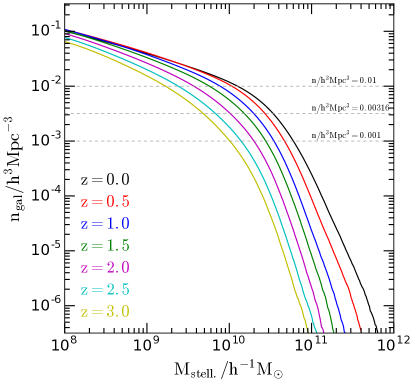
Figure 1: The cumulative stellar mass function (top panel) and the cumulative SFR function (bottom panel) predicted by the G13 SAM for different redshifts (as marked). The dashed horizontal lines indicate the number densities of the samples used in this work.

2.3.2 Classification by halo properties

To investigate assembly bias we define subsets of the fixed number density galaxy samples by selecting haloes using two different intrinsic or secondary properties: formation time (age) and concentration.

We define the formation time of a halo as the redshift when its main progenitor reaches half of the halo’s present-day mass for the first time. This definition is commonly used in the study of assembly bias (e.g., Gao et al. 2004; Gao, Springel & White 2005; Croton, Gao & White 2007, Z18). We note that the formation time of a halo is calculated at each redshift independently. We calculate the formation time using the merger trees available in the database and linearly interpolate the mass of the haloes between snapshots.

The other halo property we consider is the concentration. The halo concentration characterizes the density profile. It is canonically defined as $c_{\rm vir}=r_{\rm vir}/r_{\rm s}$, where $r_{\rm vir}$ is the virial radius of the halo and $r_{\rm s}$ is the inner “transitional” radius appearing in the Navarro, Frenk & White (1996) profile, at which the density profile changes slope. It is often alternatively defined via the rotation curve of the halo, as the ratio between $V_{\rm max}$ and $V_{\rm vir}$, where $V_{\rm max}$ is the peak value of the rotation curve, $V^{2}_{\rm c}=G\ M(r)/r$, and $V_{\rm vir}$ the virial velocity of the halo, $V_{\rm vir}\equiv V_{c}(r_{\rm vir})$ (Bullock et al. 2001; Gao & White 2007). We utilize the latter definition here, which is directly calculable from simulation data and does not require any model fitting.

In order to explore the variation in clustering and halo occupation with halo age and concentration, following Z18, we rank the haloes by these properties and identify the 20 per cent oldest and youngest haloes (based on their formation time) and (separately) the 20 per cent of haloes that are most or least concentrated. These divisions are made in 0.1 dex bins of halo mass, so as to factor out the influence of the changing halo mass function on these properties; the 20 per cent extremes of the distribution set up in this way effectively have the same mass function as the overall sample. We also tested using binnings of 0.05 and 0.2 dex in halo mass finding no difference in our main results.

2.4 The HOD and the correlation function

To study the impact of assembly bias on galaxies we measure the halo occupation functions and the correlation functions for the various halo and galaxy samples.

The HOD formalism describes the “bias” relation between galaxies and mass at the level of individual haloes allowing us to characterize the galaxy-halo connection. The key ingredient is the halo occupation function, $\langle N(M_{h})\rangle$, which represents, for a given galaxy sample, the average number of galaxies per halo as a function of halo mass (loosely referred to here also as the HOD). The commonly assumed shape for the halo occupation function is motivated by predictions of physical models such as SAMs and hydrodynamic simulations (Berlind et al. 2003; Zheng et al. 2005). When inferring the HOD it is often useful to consider separately the contribution from central galaxies and that of the additional satellite galaxies populating the halo (Kravtsov et al. 2004; Zheng et al. 2005). For stellar mass (or luminosity) threshold galaxy samples, the expected form of the central galaxies occupation function is a smoothed step function and roughly a power-law for the satellites. For samples defined by SFR or color, the shape of the halo occupation function is more complex to account for the paucity of blue/star forming centrals in massive haloes (e.g., Zehavi et al. 2005; Geach et al. 2012; Contreras et al. 2013; Gonzalez-Perez et al. 2018). We emphasize that the HODs presented in this work are all calculated directly from the SAMs, rather than inferred from the clustering, as is commonly done with observational data.

The correlation function (CF) is the most fundamental measure of the spatial distribution of haloes and galaxies. It is defined as the excess probability of finding a pair of objects at a given separation compared to a random distribution. Following Gao & White (2007) and Z18, whenever we measure the CF for the full galaxy sample we calculate the auto CF (the correlation of a given sample of objects with respect to the same sample). In contrast, when we measure the CF of a subsample of galaxies (e.g., the ones associated with the 20 per cent earliest-formed haloes) we measure the cross CF between this sample and the full galaxy sample. As explained in Z18 (see specifically their Appendix B) using the cross CF increases the signal-to-noise of the measurements and facilitates the interpretation of the results compared with the use of the auto CF of the subsamples.

3 The evolution of halo assembly bias

There are two basic ingredients necessary for galaxy assembly bias: (i) halo assembly bias, namely the dependence of halo clustering on halo properties other than mass, and (ii) the variation in the galaxy content of haloes with these properties, which we refer to as the occupancy variation (see Z18). Galaxy assembly bias requires both effects to be present. In this paper, we study how halo assembly bias, the occupancy variation and the resulting galaxy assembly bias evolve with time. This will provide further insight into the nature and origin of assembly bias and may guide attempts to detect it in observational galaxy samples. We show the evolution of halo assembly bias in this Section. The evolution of the occupancy variation is discussed in Section 4, and the evolution of galaxy assembly bias is presented in Section 5.

First we look at the evolution of halo assembly bias in the dark matter-only $N$-body simulation without reference to the SAM galaxies. We begin with a visual inspection of the distribution of haloes in the simulation. Fig. 2 shows haloes in a slice of the Millennium-WMAP7 simulation at $z=0$ and $z=3$, distinguishing between those with early and late formation times and also those with high and low concentrations. Starting with the halo age dependence at $z=0$ (Fig. 2, top-left double panels), we see that while both early-formed and late-formed haloes trace the same cosmic web, the early-formed haloes present a sharper view of the web and appear somewhat more clustered. The view of the cosmic web when highlighting the extremes of halo concentration at $z=0$ (Fig. 2, top-right panels) is reminiscent of that using halo formation time, though the clustering differences are slightly less apparent in this case. The bottom half of Fig. 2 shows the distribution of haloes chosen similarly, but now at $z=3$. As expected, the haloes overall appear less clustered than at $z=0$. The differences between the early-formed and late-formed haloes (bottom-left panels) are much smaller in this case, and interestingly for the concentration (bottom-right panels), it appears that the haloes with low concentration are in fact now more clustered than the ones with high concentration. We quantify all of the trends discussed above shortly below using the CF.

These results are in agreement with those of Gao & White (2007), who found that the halo assembly bias signal does not depend on redshift when the halo samples are selected using a fixed cut in peak height ($\nu=\delta_{c}/\sigma(M_{h})$, where $\sigma(M_{h})$ is the root mean square linear overdensity within a sphere with mean mass $M_{h}$, and $\delta_{c}(z)$ is the linear overdensity threshold for collapse at redshift z). For an increase in the peak height from $\nu=0.5$ to $\nu=1.55$ (the peak height values of the minimum halo mass of our simulation at $z=0$ and $z=3$, respectively), Gao & White (2007) found that the difference in the clustering signal between early and late-forming haloes decreases (with early formed haloes being more clustered at low $\nu$). For haloes selected by their concentration, they showed that at low peak height, high concentration haloes are more correlated than late forming, low concentration haloes, and for high peak height, low concentration haloes are more correlated than high concentration haloes. These results are equivalent to the redshift evolution trend found for a fixed halo mass cut. The same can be concluded if a fixed cut in the nonlinear mass for collapse is used (Wechsler et al. 2006).

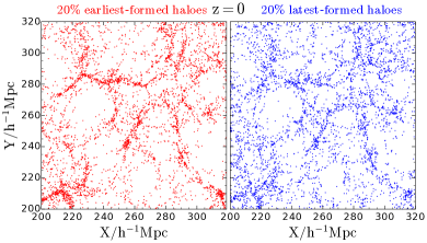
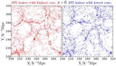
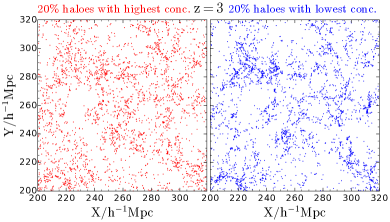
Figure 2: Left panels: A slice of $120x120x10h^{-1}\,{\rm Mpc}$ from the Millennium-WMAP7 simulation at $z=0$ (top panels) and $z=3$ (bottom panels). The red dots show the 20 per cent of haloes with the highest formation redshifts while the blue dots show the 20 per cent with the lowest formation redshifts from the full halo sample. Right panels: the distribution of haloes using red for the 20 per cent with the highest concentrations and blue for the 20 per cent with the lowest concentrations.

To better understand how the age and concentration of haloes correlate with one another at different redshifts, Fig. 3 shows the joint distribution of halo concentration and formation time at $z=0$ (left) and $z=3$ (right). We show both the distribution of the full set of haloes (contours) and the median concentration as a function of halo age for three narrow bins of halo mass (lines and errorbars). The jags in the contours in the $z=3$ panel are artificial being caused by the limited time resolution of the Millennium-WMAP7 simulation outputs at high redshift. At $z=0$ there is a clear trend of concentration increasing with formation redshift (as shown by the solid lines). On the other hand, at $z=3$ there is little variation of halo concentration with formation redshift which suggests that the assembly bias effect with concentration and halo age might be different. Xu & Zheng (2018) also look at the correlation of halo bias with different secondary halo properties (including formation time and concentration). They show that this correlation changes dramatically with halo mass. Therefore, it is unsurprising that the evolution of the clustering signal with formation time and concentration of the halo is different (see also Mao, Zentner & Wechsler 2018 who studied the dependence of clustering on several halo secondary properties).

The concentration of haloes with a small number of particles (fewer than 200 particles or $M_{h}<10^{11.26}h^{-1}{\rm M_{\odot}}$, ie. the red lines in Fig. 3) could be underestimated due to resolution effects (Trenti et al. 2010; Paranjape & Padmanabhan 2017). Most of the following analysis uses halo masses above this threshold and ranks samples in halo concentration at fixed mass, rather than using its actual value; we expect that our results should be unaffected by this possible source of systematics.

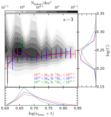
Figure 3: Halo concentration plotted as a function of formation redshift for haloes in the Millennium-WMAP7 simulation at $z=0$ (left) and $z=3$ (right). The contours represent the density of haloes as labelled by the key at the top of each panel. The solid red, blue and green lines represent the median concentration as a function of formation redshift for halo masses in the ranges $10^{11}h^{-1}{\rm M_{\odot}}\ -\ 10^{11.2}h^{-1}{\rm M_{\odot}}$ (red line), $10^{12}h^{-1}{\rm M_{\odot}}\ -\ 10^{12.2}h^{-1}{\rm M_{\odot}}$ (blue line), and $10^{13}h^{-1}{\rm M_{\odot}}\ -\ 10^{13.2}h^{-1}{\rm M_{\odot}}$ (green line). The shadowed region is computed using all the haloes in the simulation. Haloes with fewer than 200 particles ($10^{11.26}\ h^{-1}M_{\odot}$, ie. the red line) might underestimate the halo concentration due to resolution effects (see text for more details). The bars indicate the $20$ per cent $-$ 80 per cent range of the distribution. The lower panels in both cases show the distribution of haloes as a function of formation redshift and the side panels show the distribution as a function of concentration.

We now look into the CF of halo samples with different concentrations and formation times for a fixed number density after rank ordering the haloes in decreasing mass at $z=0$ and $z=3$ (Fig. 4). We use a halo number density of $n=0.00618\,h^{3}\,{\rm Mpc}^{-3}$, which is comparable to the number density of central galaxies in the $n=0.01\,h^{3}\,{\rm Mpc}^{-3}$ galaxy sample (when selecting galaxies by their stellar mass). The equivalent halo mass (peak height) cut for these samples are $10^{11.75}\ h^{-1}M_{\odot}$ (0.76) for $z=0$ and $10^{11.24}\ h^{-1}M_{\odot}$ (2.01) for $z=3$. In each subplot of Fig. 4, the black line in the top panel denotes the auto CF of the full halo sample, while the red (blue) lines correspond to the cross CF of the full sample with the 20 per cent oldest (youngest) haloes in the top row of the figure, or the 20 per cent highest (lowest) concentration haloes in the bottom row (see § 2.4).

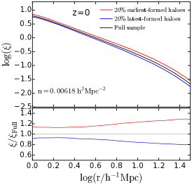
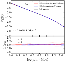
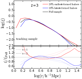
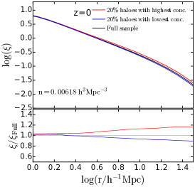
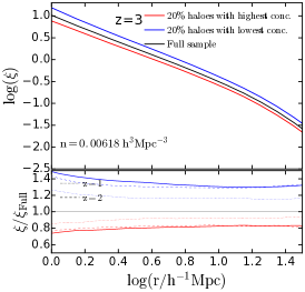
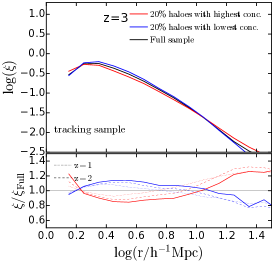
Figure 4: (Left) The halo cross CF (coloured lines) and the auto CF (black lines) at $z=0$, for a halo number density of $0.00618\ h^{3}\,{\rm Mpc}^{-3}$. The top and bottom panels show the contribution of haloes with high and low formation redshifts and concentrations, respectively. (Middle) Same as the left panel, but for haloes at $z=1,2,3$. (Right) The halo cross CF and the auto CF of the main progenitors of the $z=0$ haloes at $z=1,2$ and $3$. For this plot only, the classification in terms of age and concentration is made using the descendants of these haloes at $z=0$.

We find that at $z=0$, haloes with early formation times and high concentrations are more clustered than ones with late formation times and low concentrations. This is the well-studied behavior of halo assembly bias (e.g., Gao, Springel & White 2005; Wechsler et al. 2006; Gao & White 2007). The halo assembly bias effect, as reflected by the clustering differences, is slightly stronger for the case of halo formation time than for halo concentration and extends to smaller separations. We note that as we are measuring here halo (instead of galaxy) clustering, the scales involved are all in the so-called 2-halo regime. At higher redshift (e.g., $z=3$) there is no difference in the clustering measured for haloes at the extremes of the formation time distribution and low concentration haloes are more clustered than high concentration haloes, reversing the trend seen at the present day.

We reach the same conclusions as already inferred from Fig. 2, namely that the halo assembly bias signal (i.e. the difference between the red and blue lines) decreases with increasing redshift for halo samples selected by age. For concentration, the evolution of halo assembly bias is stronger in the sense that the clustering differences reverse at high redshift. These trends are in agreement with the evolution of the halo assembly bias signal found in the original Millennium simulation by Gao & White (2007) where they found the same trends when the peak height increases from 0.76 to 2.01, that is the increase of peak height from our samples between $z=0$ and $z=3$ (see Wechsler et al. 2006 for a comparison using the nonlinear mass for collapse.)

To understand the origin of this difference between using age and concentration as the secondary parameter we show in the right panel of Fig. 4 the CF of the main progenitors of the $z=0$ haloes selected at $z=1,2$ and $3$. We call this sample the ‘tracking sample’. For this sample only, the secondary property halo labels (i.e. in terms of the extremes of concentration or formation time) refer to the $z=0$ descendants. We find different trends for different scales. At large scales ($>10\ h^{-1}{\rm Mpc}$), the tracking sample shows the same clustering trend as their descendants at $z=0$ but with a higher amplitude. The behaviour of the tracking sample cannot be easily related to the Wechsler et al. (2006) or Gao & White (2007) results, since there is no fixed mass cut (or peak height or nonlinear mass for collapse) in the tracking sample. We interpret this non-evolution in the halo clustering as a negligible change in the comoving position and abundance of the haloes in this redshift range. This means that the evolution of halo assembly bias is not caused by a change in the clustering of haloes with extreme values of formation time or concentration. Instead we attribute the evolution of the assembly bias signal at a fixed halo number density to a shift in the ranking of haloes according to their mass and secondary property. This means that, for example, haloes with the highest concentrations at $z=0$ are not necessarily the ones with the highest concentrations at $z=3$.

We demonstrate this shift in the ranking of the haloes in Table 1. Here we show that fewer than $40$ per cent of the progenitors of $z=0$ haloes were part of the original sample at $z=1$. At $z=3$ this number decreases to $\sim 20$ per cent. This shift also explains the different evolution of halo samples selected by age and concentration. Table 2 shows that while at $z=0$ there is a $\sim 40$ per cent overlap between members of the early (late) formation time halo sample and the high (low) concentration halo sample this number decreases to $\sim 10$ per cent at $z=3$.

	z=0	z=1	z=2	z=3
Early forming	100	29	23	22
Late forming	100	18	18	17
High conc.	100	37	23	19
Low conc.	100	22	14	11

Table 1: The progenitors of a 100 representative haloes from the $n=0.00618\ h^{3}\,{\rm Mpc}^{-3}$ sample at $z=0$, drawn from the early and late formation time, high and low concentration samples, that were part of those samples at $z=0,1,2$ and $3$.

	z=0	z=1	z=2	z=3
Early forming - high conc.	40	29	19	10
Late forming - low conc.	41	27	17	13

Table 2: The haloes in common in a representative sample of 100 haloes for a fixed number density of $n=0.00618\ h^{3}\,{\rm Mpc}^{-3}$ in the early formation time - high concentration samples and in the late formation time -low concentration samples. The numbers are calculated as the ratio between the number of haloes in the interception of the two samples ($\rm A\cap B$) and the number of haloes in the union of both samples ($A\cup B$).

Different trends are seen at intermediate and small separations in the right panels of Fig. 4. The progenitors of early formation time and high concentration haloes are more correlated on small scales and less correlated on intermediate scales (compared to haloes with late formation times and low concentrations). These are not the focus of our work presented here, and we provide just some heuristic considerations. As early-formed haloes grow faster at higher redshifts it may be expected that they exhibit stronger clustering on small scales at $z=3$ (since they accrete mass from nearby structures). The stronger clustering on intermediate scales for haloes with late formation times may be explained in terms of these haloes accreting more mass at lower redshifts and the structures that will merge with these haloes being in their vicinity but not immediate proximity.

Since at $z=0$ there is a $\sim 40$ per cent overlap between halo samples selected by age and concentration (Table 2) we can assume this explanation is also valid for the main progenitors of the haloes selected by concentration.

One might be concerned that the agreement between the correlation functions of early and late formation time haloes in the top-middle panel of Fig. 4 could be an artifact of the limited time resolution of the Millennium-WMAP7 simulation at high redshifts. To check this we also calculated the correlation functions using the P-Millennium simulation (Baugh et al. 2018), a dark matter only simulation with over four times as many snaphots as the Millennium-WMAP7 run and with a better mass resolution. We find the same trends as those presented in this work, confirming that our results are not a product of the finite time resolution of the dark matter simulation used.

4 The occupancy variation evolution

In this section we show the evolution of the occupancy variation in the SAM, i.e., how the dependence of the HOD on a secondary halo property varies with time. This may provide us more insight into the nature and origin of this phenomena.

Z18 showed that in SAMs, when selecting galaxies at $z=0$ by their stellar mass, the predicted HOD depends on halo formation time as well as halo mass. They found that haloes with early formation times tend to start being populated by central galaxies (the main galaxy of a dark matter halo) at lower masses than those with late formation times, but they have a lower number of satellites. Artale et al. (2018) show that this is also the case in hydrodynamic simulations. We find that the above results also hold for other redshifts. This is shown, for example, in Fig. 5, where we plot the HOD at $z=1$ for $n=0.01\,h^{3}\,{\rm Mpc}^{-3}$ for galaxies ranked by their stellar mass. The occupancy variation for both central and satellite galaxies is clearly evident.

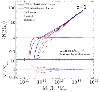
Figure 5: (Top) The halo occupation distributions at $z=1$ for a galaxy sample with $n=0.01\ h^{3}\,{\rm Mpc}^{-3}$. The lines show the contribution of all galaxies (solid), centrals galaxies only (dotted) and satellite galaxies only (dashed). The red and blue lines show the halo occupation distributions for the $20$ per cent earliest and latest forming haloes, respectively. The shaded region represents the jackknife errors using 10 subsamples, and is effectively negligible over most of the range. (Bottom) The ratio between the different halo subsets (with the oldest haloes in red and youngest ones in blue) and the full sample HOD for central galaxies (dotted line) and satellites (dashed line). The lines are plotted only when there are at least 20 haloes per halo mass bin of 0.1 dex width.

Fig. 6, shows the HOD for $z=0$ (top) and $z=3$ (bottom) for the same sample selection. In the left panels of Fig. 6 the lines represent the contribution from the $20$ per cent of haloes with the earliest (red) and latest (blue) formation times, while the right panels show the contribution from the haloes with the $20$ per cent highest and lowest concentrations. We remind the reader that these halo subsamples are constructed by selecting the haloes in narrow bins of halo mass. At $z=0$, the predictions for the high (low) concentration samples are similar to those with early (late) formation times. This is consistent with what we found in Section 3, that the behaviour of these samples in terms of clustering is similar at $z=0$, but now extended to the halo occupation with galaxies. This similarity is no longer present at $z=3$. At this redshift, the occupancy variation for haloes selected by their age is qualitatively similar to that at $z=0$ (and at $z=1$; see Fig. 5). For haloes selected by concentration, the occupancy variation decreases somewhat for the satellite galaxies and it almost disappears for the central galaxies as we go to $z=3$. These trends also hold for other number density samples.

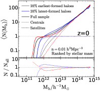
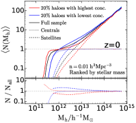
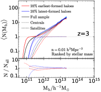
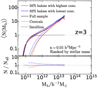
Figure 6: (Left) Same as Fig. 5 but for $z=0$ (top) and $z=3$ (bottom). (Right) Same as the left panels, but for haloes selected by concentration instead of formation time.

We repeat the above analysis for galaxies selected by SFR in Fig. 7. The overall shape of the HOD at $z=0$ for SFR-selected galaxies is different than for galaxies selected by stellar mass due to the tendency of high mass halos to host non star forming (red) central galaxies, as discussed in Section 2.4. Interestingly, the “dip” feature diminishes as one goes toward higher redshifts, possibly due to having less time for quenching mechanisms to occur. By $z=3$ the overall shape of the HOD, and in particular the central galaxies contribution, is very similar for the SFR-selected galaxy samples and the stellar mass selected samples (see also Orsi et al. 2008). We have verified that the transition in the shape of the HOD between $z=0$ and $z=3$ is smooth with increasing redshift. A large set of HOD measurements for different redshifts and number densities is being released with this paper (see Appendix A for more details).

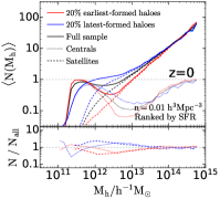
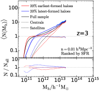
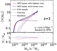
Figure 7: Same as Fig. 6 but for galaxies selected by their SFR instead of stellar mass.

At $z=0$, for the SFR-selected galaxy samples, early forming and high concentration haloes have a lower number of satellite galaxies compared to haloes with late formation times or low concentrations (same as for galaxies selected by stellar mass). For the central galaxies, at low halo masses, early forming and high concentration haloes have a larger number of central galaxies, while for higher halo masses they have a lower number of central galaxies compared to haloes with late formation times or low concentrations. The latter trend perhaps arises since the central galaxies in the early-formed high-mass halos have more time to be impacted by star formation quenching. At $z=3$, the HODs for galaxies selected by SFR display the same trends as those for galaxies selected by stellar mass. The occupancy variation (i.e. the difference between the red and blue lines) stays roughly constant for haloes selected by age. The occupancy variation with halo concentration decreases with redshift for the HOD of the satellites and nearly diminishes for that of the central galaxies.

The full redshift evolution of the occupancy variation is captured in Fig. 8 and Fig. 9, where we show the ratios of the HODs (as in the bottom subpanels of Fig. 5-7) for halos selected by age and concentration at all redshifts explored, for galaxies selected by stellar mass and SFR, respectively. Here we corroborate that, for galaxies selected by stellar mass, the magnitude of the central galaxies occupancy variation is constant with redshift for haloes selected by age and it significantly decreases with increasing redshift (nearly diminishing by $z=3$) for haloes selected by concentration. The occupancy variation for the satellites part of the HOD progressively decreases for either age or concentration. The overall shift of the ratios toward lower halo mass with increasing redshift reflects the expected redshift evolution of the HOD (as studied for example by Contreras et al. 2017; see their Fig. 5). For SFR selected galaxies (Fig. 9), the occupancy variations decrease for both age and concentration, with a more pronounced trend for the latter.

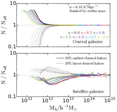
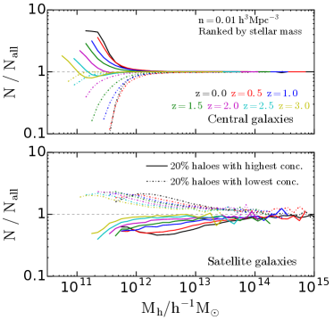
Figure 8: Same as the bottom sub-panels of Fig. 5, but now combined for $z=0,0.5,1,1.5,2,2.5$ and $3$. The top panels presents the central galaxies contribution and the bottom panels is the satellites contribution. The two left panels show, as solid (dotted) lines, the ratio between the HOD of the $20$ per cent earliest (latest) formation time haloes and the full HOD, and in the right panels, the ratio of the HOD of the $20$ per cent high (low) concentration haloes and the full HOD, for galaxies selected by their stellar mass.

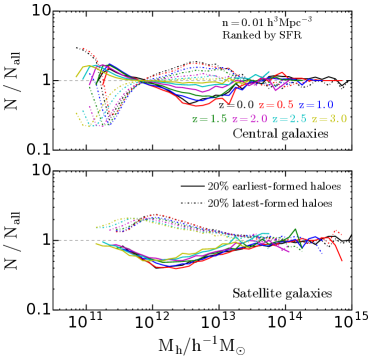
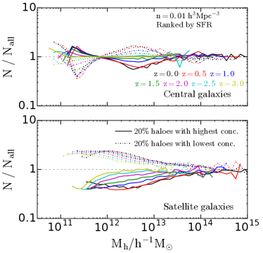
Figure 9: Same as Fig. 8 but for galaxies selected by their SFR.

The different evolution of the occupancy variation with age and concentration indicates a different origin for these two effects. Even though they appear similar at $z=0$, they evolve differently. We will further investigate their nature and origin in future work (Zehavi et al., in prep.). It is interesting to note that the evolution of the occupancy variation shows different trends compared to the evolution of the halo assembly bias found in Section 3, where the signal decreased for the halo samples selected by age but not for those selected by concentration as in the occupancy variation case. Both effects will influence the evolution of the galaxy assembly bias signal, as we will now show.

5 The evolution of galaxy assembly bias

In this section we show the effect of assembly bias on the galaxy correlation function at different redshifts. As we did in Section 3, we measure the auto CF for the full galaxy sample as well as the cross CF of the full sample with the given subsample (e.g. early/late formed haloes).

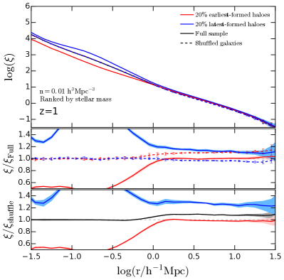
Figure 10: The auto-correlation and cross-correlation functions at $z=1$ for a stellar mass selected galaxy sample with number density of $0.01\ h^{3}\,{\rm Mpc}^{-3}$. Dashed lines correspond to the shuffled galaxy sample (i.e., without occupancy variation) and solid lines represent the original sample. The red (blue) lines show the cross-correlation function between the galaxies that populate the $20$ per cent earliest (latest) forming haloes and the full galaxy sample. The black lines show the auto-correlation function for the full sample. The top panel shows the different correlation functions, the middle panel shows the cross-correlation functions (red and blue lines) divided by the auto-correlation function (black), and the bottom panel shows the ratio between different correlation functions from the model and the ones from the shuffled sample. The shaded region and errorbars represent the jackknife errors calculated using 10 subsamples.

To study the impact of assembly bias on the CF we shuffle galaxies among haloes of the same mass, following the approach of Croton, Gao & White (2007) and Z18. This consists of taking all haloes in a given bin of halo mass (0.1 dex wide in our case; we also tested using a bin width of 0.05 and 0.2 dex and found no major difference in our results) and randomly reassigning the galaxy population between these haloes. Central galaxies are located at the position of the central galaxies they replace (except if there is no galaxy in a halo; in which case the new galaxy is located at the potential minimum of the halo). The satellite galaxies are moved together with their original central galaxy and retain the same relative positions to it in their new halo. The shuffling removes any potential connection to the assembly history of the halos, and effectively transforms the HOD of any halo subsample (e.g., for a range of halo formation times or concentrations) to be the same as the total HOD (making, e.g., the red and blue lines of Fig. 5 be the same as the black line). This new galaxy sample will have, by construction, no occupancy variation.

The CFs for a stellar mass selected sample with number density $n=0.01\ h^{3}\,{\rm Mpc}^{-3}$ at $z=1$ is shown in top panel of Fig. 10. The auto CF of the full sample is shown in black, and the red and blue lines are the cross CF for the $20$ per cent earliest and latest forming haloes, respectively. The dashed lines show the CF for the shuffled samples. The shaded region and errorbars represent the jackknife errors calculated using 10 realisations for the real and the shuffled samples. The middle panel shows the ratios between the cross CF of the subsamples and the auto CF of the full sample, for both original (solid) and shuffled (dashed) galaxy samples. The bottom panel shows the ratios between the different CFs measured for the original (unshuffled) galaxy samples and the corresponding shuffled ones.

A value above unity for the black line in the bottom panel of Fig. 10 indicates that the original sample has a larger CF than that measured for the shuffled sample. These differences are the manifestation of galaxy assembly bias (Croton, Gao & White 2007). As explained in Z18, this arises from the combined effect of the occupancy variation and halo assembly bias. The central galaxies occupancy variation indicates a preferential occupancy of early-formed halos. These halos are more clustered, thus leading to a stronger clustering signal on large scales. The significant clustering differences on small scales come about from the satellites occupancy variation, where the increased number of satellites in late-forming halos gives rise to a stronger clustering in the 1-halo regime.

It is interesting to note that the clustering of galaxies in the late-forming haloes is stronger on large scales than that for galaxies in early-formed haloes, as can be seen in the middle panel of Fig. 10. This is the opposite to the results found by Z18 at $z=0$, implying that trend evolves with redshift. This again arises from the inter-related effects of halo assembly bias and the occupancy variation. The dashed lines in the middle panel correspond to the shuffled galaxy samples, and reflect the same halo assembly bias trends seen in Fig. 4, modulated by satellite galaxies. The central occupancy variation acts to slightly increase this ratio for the galaxies in late-forming haloes and decrease it for the galaxies in early-formed halos (see corresponding discussion in Z18, specifically their §5.3), thus likely resulting in the reversed clustering trend seen.

The evolution of this ratio is individually presented Fig. 11. The left panels show the ratio between the CF measured for galaxies in haloes with the 20 per cent earliest/latest formation times and the CF of the full sample, for $z=0,1,2$ and $3$. The panels on right show the same but for haloes selected by concentration. Solid lines show the original SAM galaxies and dashed lines show the shuffled sample results (i.e., with no occupancy variation). For the shuffled samples, we can see that the difference between the CFs of galaxies in the earliest/latest-forming haloes decreases with increasing redshift while the difference for haloes with the highest/lowest concentrations is reversed, with increasingly stronger clustering found for the haloes with a lower concentration. These trends are consistent with the evolution of the halo assembly bias signal shown in Section 3, where we found a decrease (flip) of the of the difference in clustering on large scales for haloes selected by age (concentration). At high redshift, the differences in the clustering of the SAM galaxies in early and late formed haloes come mostly from the occupancy variation. This is opposite to the situation of galaxies that live in high and low concentrated haloes, where the differences in their clustering come mostly from halo assembly bias.

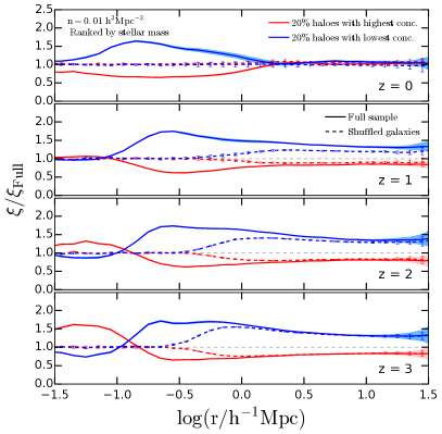
Figure 11: The same as the middle panel of Fig. 10, for galaxies selected by their stellar mass with a number density of $0.01\ h^{3}\,{\rm Mpc}^{-3}$, at $z=0,1,2$ and $3$. Halo samples selected by their formation redshift are shown on the left hand side and by their concentration on the right. Please note that a larger y-axis range is shown here versus the one in Fig. 10.

For the galaxy population predicted by the SAM, galaxies in haloes with late formation times or low concentrations show stronger large-scale clustering at higher redshifts. For the concentration case, the clustering signal becomes identical to that measured for the shuffled galaxies. This is expected since, as shown in Section 4, the occupancy variation of haloes with concentration decreases strongly with increasing redshift. For galaxies in haloes selected by formation time, the clustering of the galaxies in the latest forming haloes is stronger than the shuffled galaxies, while for the galaxies in the earliest-forming haloes it is lower than for the shuffled case. This is again consistent with what we found in § 4, with the occupancy variation with age persisting to higher redshifts, with (at each redshift) late (early) formation effectively shifting the occupation toward higher (lower) halo masses, thus changing the clustering.

On small scales, the dashed lines in Fig. 11 are identical for both age and concentration, since there is no halo assembly bias in that regime (1-halo scales). The SAM galaxies in late-forming haloes are more correlated than those in early-forming haloes on small scales, at all redshifts. This is due to the increased number of satellites in early versus late forming halos, which persists at all redshifts (as seen in Fig. 8). Galaxies selected by halo concentration exhibit a similar behavior – galaxies in low concentration haloes are more clustered than those in high concentration ones – at small-to-intermediate scales. On very small scales (below $\sim 0.1h^{-1}\,{\rm Mpc}$), though, this trend flips. One might have expected the same small-scale behaviour with concentration due to the similar satellite occupancy variation. However, the concentration differences impact the clustering as well. E.g., for the low-concentration sample, even with more satellite galaxies, they are likely less concentrated (since they trace the dark matter distribution) and as a consequence, less clustered on very small scales.

In Fig. 12 we show, for completeness, the corresponding evolution of the CFs for galaxies selected by their SFR. We obtain the same trends found for galaxies selected by stellar mass. We also analysed other number density samples and found similar results for the evolution of the galaxy CFs.

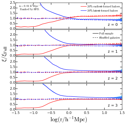
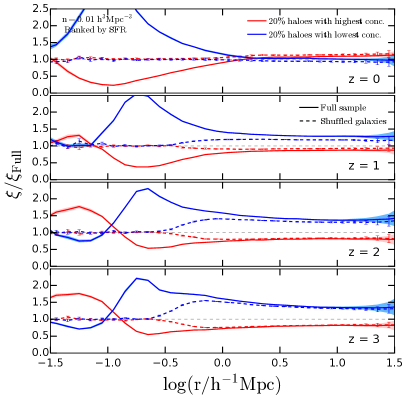
Figure 12: The same as Fig. 11, but now for galaxies selected by their SFR instead of stellar mass.

Finally, we consider the evolution of the galaxy assembly bias signal. As previously mentioned, galaxy assembly bias is quantified in terms of the ratio between the CF of a galaxy sample and that of a shuffled sample, where the relation to halo assembly has been erased, as shown by the black line in the bottom panel of Fig. 10. Fig. 13 presents our measurements for three different number densities ($n=0.01$, $0.00316$ and $0.001\,h^{-3}\,{\rm Mpc}^{3}$) over a range of redshifts, for galaxies selected by stellar mass and SFR. We find that this clustering ratio generally decreases for higher redshifts, and for lower number densities. Interestingly, this decrease can be large enough in some of these cases so that the original sample becomes less clustered than the corresponding shuffled sample, and the clustering difference changes sign and continues growing in magnitude. This typically occurs for lower number densities and at high redshifts. This ratio is overall lower for the galaxy samples selected by their SFR rather than stellar mass. Nonetheless, the trends with redshift and number density persist for these SFR selected samples,

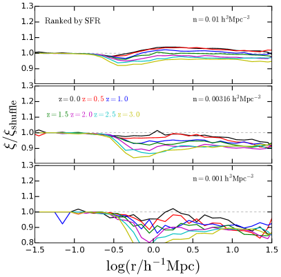
Figure 13: The ratio between the correlation function of the full galaxy sample and the corresponding shuffled sample (equivalent to the black line in the bottom panel of Fig. 10) for three different number densities of $0.01\ h^{3}\,{\rm Mpc}^{-3}$ (top), $0.00316\ h^{3}\,{\rm Mpc}^{-3}$ (middle) and $0.001\ h^{3}\,{\rm Mpc}^{-3}$ (bottom), and for $z=0,0.5,1,1.5,2,2.5$ and $3$ as labelled. Galaxies selected by stellar mass are shown on the left hand side while galaxies selected by SFR are shown on the right.

Our results are in qualitative agreement with those found by Hearin et al. (2016; their Fig. 8) over the limited redshift range they explore ($0<z<1$). However, we note that Hearin et al. compare samples with the same stellar mass thresholds at the different redshifts, not accounting for any stellar mass evolution. Effectively, this amounts to probing more massive galaxies (lower number densities) at higher redshifts, and thus it is impossible to separate the evolution they find from the expected number density dependence.

Again, the impact of assembly bias on galaxy clustering arises from the combined contributions of the occupancy variation and halo assembly bias. At relatively low redshift for the stellar mass selected samples, these typically combine to produce an increased clustering (see the discussion following Fig. 11 and in Z18). For example, using our results in the previous sections for $n=0.01h^{3}\,{\rm Mpc}^{-3}$, we can explain the behaviour exhibited in the top-left panel of Fig. 13. As we saw earlier for the halo age case, the level of halo assembly bias decreases while the level of the central galaxies occupancy variation remains similar, leading to a diminishing galaxy assembly bias effect. For lower number densities at high redshifts, halo assembly bias reverses sense (in a similar manner to concentration) such that early-formed halos become less clustered than the late-formed ones, and this gives rise to the reversed sense of galaxy assembly bias in those cases.

One could have a-priory envisioned a scenario in which the stochasticity involved in the galaxy formation processes would serve to weaken galaxy assembly bias over time. Alternatively, one might have expected the signature to grow with time (i.e., diminish as one goes to higher redshift), due to the hierarchical growth of structure. However, it seems that the evolution of assembly bias is far more intricate. The overall trend we find is that the CFs ratio monotonically increases with time (or decreases with increasing redshift; Fig. 13). This leads to a change in the sign of the effect, i.e., whether the clustering of the galaxy sample is stronger or weaker due to assembly bias effects, as well as a shift in whether the magnitude of this clustering difference decreases or increases with time. This gets more complex as the amplitude of the clustering ratio varies with the specifics of the galaxy selection (e.g., stellar mass or SFR) and number density, thus it is non-trivial to predict which galaxy sample would show negligible or extreme assembly bias properties and at which redshift.

6 Summary & Conclusions

We use a state-of-the-art semi-analytic model of galaxy formation, the G13 SAM model, to study the origin and evolution of assembly bias in the galaxy distribution. We identify two separate contributions to this effect: halo assembly bias, which refers to the different clustering of haloes with different ‘secondary property’, and occupancy variation, the dependence of the number of galaxies in haloes of the same mass on a second property of the haloes. We isolate the evolution of these two effects for haloes selected by their concentration and formation redshift, two of the most common secondary properties used to measure assembly bias. The galaxy samples correspond to different number densities based on either ranked stellar mass or SFR. Our key results are shown in Figures 4, 8 and 13. We now summarise our main findings:

• At $z=0$ the concentration of dark matter haloes correlates with formation time. This correlation weakens at higher redshifts.

• Haloes at $z=0$ with high concentrations or early formation times are more clustered than those with low concentrations or late formation times. At high redshift, there are no differences in the CF measured for haloes with different formation times, but low concentration haloes are more correlated than high concentration ones.

• Haloes ranked to have an extreme concentration or formation time at a given redshift do not necessarily have the same ranking at other redshifts. We found that the main progenitors of $z=0$ haloes display clustering similar to that measured for their descendants. This means that the evolution of the halo assembly bias signal is not caused because a set of haloes (e.g., high concentration haloes) change their clustering over time, but because haloes change their ranking in terms of a secondary property.

• At $z=0$, haloes with early formation times or high concentrations are populated by galaxies starting at lower halo masses (for a fixed cut in stellar mass) but they have fewer satellite galaxies for a fixed mass compared to haloes with late formation times or low concentrations.

• For galaxies selected by SFR we generally find similar occupancy variation trends to those found for galaxies selected by stellar mass (though different shape of the HOD). Haloes with early formation times or high concentrations are first populated by galaxies at a lower mass and have fewer satellite galaxies at a given mass compared to haloes with late formation times or low concentrations. The one difference is that at higher halo masses, where the central galaxies occupation drops, there are less centrals in haloes with early formation times or high concentrations than for those with either late formation times or low concentrations.

• The occupancy variation for central galaxies in haloes with different formation times stay roughly constant as a function of redshift for a fixed galaxy number density and for galaxies selected by either stellar mass or SFR. The corresponding satellite galaxies occupancy variation decreases somewhat with increasing redshift.

• The occupancy variation for galaxies in haloes with different concentrations diminishes for the central galaxies and satellites with increasing redshift, for both stellar mass or SFR selected galaxy samples.

• The evolution of the CF of galaxy samples without occupancy variation (i.e., the shuffled samples) reflects the same trends on large scales as the evolution of halo assembly bias for haloes selected by age or concentration; the CF differences for galaxies in haloes with early and late formation times decreases with look back time, while the CF of galaxies in low-concentration haloes increases relative to the CF of galaxies in high-concentration haloes when going to higher redshifts.

• The CF of galaxies hosted by haloes with late formation times or low concentration increases relative to the CF of galaxies in haloes with early formation times or high concentrations, respectively, with increasing redshift.

• The occupancy variation tends to increase the amplitude of the CF of galaxies that live in haloes with either late formation times or low concentrations, and decrease it for galaxies that live in haloes with early formation times or high concentrations.

• Galaxy assembly bias as measured by the ratio between the CF of the model galaxies and that of the shuffled galaxies decreases with redshift, going below 1 in some cases. This CFs ratio is generally smaller for lower number densities and for SFR-selected samples.

The different evolution of halo assembly bias and the occupancy variation with age and concentration likely points to a different origin for the dependence on these two secondary parameters. This is further corroborated by their lack of correlation at high redshift. In general, we find similar trends in the evolution of assembly bias, for both the occupancy variation and galaxy assembly bias, for galaxies selected by SFR versus stellar mass. This is quite impressive considering that galaxy samples selected by stellar mass and by SFR exhibit quite different behaviours in the SAMs (Contreras et al. 2013, 2015), and may be relevant for upcoming surveys.

The results shown here will help to inform theoretical models of assembly bias and the development of observational tests to detect its existence (or absence) in the Universe. They can also be used to construct improved mock galaxy catalogues incorporating assembly bias (as standard HOD mocks do not include this effect). For these purposes we are releasing all the HODs and occupancy variation measures obtained in this work, as well as parametrised fits for them (see Appendix A for more details).

Appendix A HOD catalogues

To facilitate the creation of mock galaxy catalogues with occupancy variation, which can be used for the creation of mocks with galaxy assembly bias, we are making public the HODs calculated in this work. The HODs are calculated for the following number densities, $n=0.0316,0.01,0.00316,0.001,0.000316$ and $0.0001\,h^{3}\,{\rm Mpc}^{-3}$, for galaxies ranked either by stellar mass or SFR. The following redshifts are used, $z=0,0.5,1,1.5,2,2.5$ and $3$, and the haloes are selected in 10 bins of ranked age and concentration. This yields more than 1,800 HODs in total. This material can be found at https://github.com/hantke/-HOD_Extractor2

Additionally, we provide in this same repository the HOD fitting parameters for all galaxy samples selected by stellar mass, for the commonly used 5-parameter model introduced by Zheng et al. 2005. The HOD parameters of the galaxies selected by SFR can not be well represented by this standard parametrization (see, e.g., Contreras et al. 2013) and will be investigated further in future work. The 5-parameters model is given by

$$\langle N_{\rm gal}(M_{\rm h})\rangle=\langle N_{\rm cen}(M_{\rm h})\rangle+\langle N_{\rm sat}(M_{\rm h})\rangle,$$ (1)

with

$$\langle N_{\rm cen}(M_{\rm h})\rangle=\frac{1}{2}\left[1+{\rm erf}\left(\frac{\log M_{\rm h}-\log M_{\rm min}}{\sigma_{\log M}}\right)\right]$$ (2)

and

$$\langle N_{\rm sat}(M_{\rm h})\rangle=\left(\frac{M_{\rm h}-M_{\rm cut}}{M^{*}_{1}}\right)^{\alpha},$$ (3)

where $M_{\rm h}$ is the host halo mass and ${\rm erf}(x)$ is the error function,

$${\rm erf}(x)=\frac{2}{\sqrt{\pi}}\int_{0}^{x}e^{-t^{2}}{\rm d}t.$$ (4)

$M_{\rm min}$ is the mass where, on average, half of the haloes are occupied by a central galaxy (i.e., $\langle N_{\rm cen}(M_{\rm min})\rangle=0.5$); $\sigma_{\log M}$ characterises the width of the transition from zero to one central galaxy per halo, where $\sigma_{\log M}=0$ represents a vertical step-function transition; $\alpha$ is the slope of the satellite HOD power-law; $M_{\rm cut}$ is the minimum halo mass at which haloes can host a satellite galaxy and $M^{*}_{1}$ is the normalization. Note that we provide instead the value of a related parameter, $M_{1}$, the halo mass where on average there is one satellite per halo (i.e., $\langle N_{\rm sat}(M_{1})\rangle=1$) and is equal to $M_{\rm cut}+M^{*}_{1}$.

As an example, we provide in Table 3 the HOD parameters for the galaxy samples with $n=0.01\ h^{3}\,{\rm Mpc}^{-3}$ at $z=0,1,2,3$ and for the $10$ per cent oldest haloes, the $10$ per cent youngest haloes, and the full halo sample. The full set of fitted parameters is provided in our public release website. Together with the HODs and their parameters (stored in two HDF5 files), we are also releasing tools to read and plot the HODs to facilitate their analysis.

		$z=0$
	$M_{\rm min}$	$\sigma_{\log M}$	$\alpha$	$M_{\rm cut}$	$M_{1}$
10$\%$ oldest haloes	11.44	0.10	1.15	11.99	12.82
All haloes	11.62	0.21	0.99	11.83	12.57
10$\%$ youngest haloes	11.92	0.30	0.84	11.74	12.31
		$z=1$
	$M_{\rm min}$	$\sigma_{\log M}$	$\alpha$	$M_{\rm cut}$	$M_{1}$
10$\%$ oldest haloes	11.36	0.16	1.07	11.97	12.57
All haloes	11.59	0.28	0.92	11.81	12.34
10$\%$ youngest haloes	11.94	0.37	0.85	11.70	12.18
		$z=2$
	$M_{\rm min}$	$\sigma_{\log M}$	$\alpha$	$M_{\rm cut}$	$M_{1}$
10$\%$ oldest haloes	11.15	0.11	1.08	11.66	12.33
All haloes	11.41	0.30	0.92	11.60	12.13
10$\%$ youngest haloes	11.74	0.34	0.86	11.46	11.97
		$z=3$
	$M_{\rm min}$	$\sigma_{\log M}$	$\alpha$	$M_{\rm cut}$	$M_{1}$
10$\%$ oldest haloes	10.89	0.13	1.01	11.47	12.07
All haloes	11.17	0.32	0.93	11.34	11.91
10$\%$ youngest haloes	11.51	0.33	0.85	11.24	11.70

Table 3: The HOD parameters described in Eqns. A1 to A4 for galaxy samples corresponding to a number density of $n=0.01\ h^{3}\,{\rm Mpc}^{-3}$ selected by stellar mass. From top to bottom we show the parameters for $z=0,\ 1,\ 2\ \&\ 3$, for the $10$ per cent oldest haloes, for the full halo sample and for the $10$ per cent youngest haloes.

References

- Abbas & Sheth (2006) Abbas U., Sheth R. K., 2006, MNRAS, 372, 1749
- Artale et al. (2018) Artale M. C., Zehavi I., Contreras S., Norberg P., 2018, MNRAS, in press
- Baugh (2006) Baugh C. M., 2006, Reports on Progress in Physics, 69, 3101
- Baugh et al. (2018) Baugh C. M. et al., 2018, MNRAS
- Benson (2010) Benson A. J., 2010, PhysRep, 495, 33
- Benson (2012) Benson A. J., 2012, NewAst, 17, 175
- Berlind et al. (2006) Berlind A. A. et al., 2006, ApJS, 167, 1
- Berlind & Weinberg (2002) Berlind A. A., Weinberg D. H., 2002, ApJ, 575, 587
- Berlind et al. (2003) Berlind A. A. et al., 2003, ApJ, 593, 1
- Bertone, De Lucia & Thomas (2007) Bertone S., De Lucia G., Thomas P. A., 2007, MNRAS, 379, 1143
- Blanton & Berlind (2007) Blanton M. R., Berlind A. A., 2007, ApJ, 664, 791
- Bond et al. (1991) Bond J. R., Cole S., Efstathiou G., Kaiser N., 1991, ApJ, 379, 440
- Bower et al. (2006) Bower R. G., Benson A. J., Malbon R., Helly J. C., Frenk C. S., Baugh C. M., Cole S., Lacey C. G., 2006, MNRAS, 370, 645
- Bullock et al. (2001) Bullock J. S., Dekel A., Kolatt T. S., Kravtsov A. V., Klypin A. A., Porciani C., Primack J. R., 2001, ApJ, 555, 240
- Busch & White (2017) Busch P., White S. D. M., 2017, ArXiv e-prints
- Campbell et al. (2015) Campbell D., van den Bosch F. C., Hearin A., Padmanabhan N., Berlind A., Mo H. J., Tinker J., Yang X., 2015, MNRAS, 452, 444
- Chaves-Montero et al. (2016) Chaves-Montero J., Angulo R. E., Schaye J., Schaller M., Crain R. A., Furlong M., Theuns T., 2016, MNRAS
- Cole et al. (1994) Cole S., Aragon-Salamanca A., Frenk C. S., Navarro J. F., Zepf S. E., 1994, MNRAS, 271, 781
- Contreras et al. (2013) Contreras S., Baugh C. M., Norberg P., Padilla N., 2013, MNRAS, 432, 2717
- Contreras et al. (2015) Contreras S., Baugh C. M., Norberg P., Padilla N., 2015, MNRAS, 452, 1861
- Contreras et al. (2017) Contreras S., Zehavi I., Baugh C. M., Padilla N., Norberg P., 2017, MNRAS, 465, 2833
- Cooper et al. (2010) Cooper M. C., Gallazzi A., Newman J. A., Yan R., 2010, MNRAS, 402, 1942
- Cooray & Sheth (2002) Cooray A., Sheth R., 2002, PhysRep, 372, 1
- Coupon et al. (2012) Coupon J. et al., 2012, A&A, 542, A5
- Croton, Gao & White (2007) Croton D. J., Gao L., White S. D. M., 2007, MNRAS, 374, 1303
- Croton et al. (2006) Croton D. J. et al., 2006, MNRAS, 365, 11
- Croton et al. (2016) Croton D. J. et al., 2016, ApJS, 222, 22
- Davis et al. (1985) Davis M., Efstathiou G., Frenk C. S., White S. D. M., 1985, ApJ, 292, 371
- De Lucia & Blaizot (2007) De Lucia G., Blaizot J., 2007, MNRAS, 375, 2
- De Lucia, Kauffmann & White (2004) De Lucia G., Kauffmann G., White S. D. M., 2004, MNRAS, 349, 1101
- Dvornik et al. (2017) Dvornik A. et al., 2017, MNRAS, 468, 3251
- Gao, Springel & White (2005) Gao L., Springel V., White S. D. M., 2005, MNRAS, 363, L66
- Gao & White (2007) Gao L., White S. D. M., 2007, MNRAS, 377, L5
- Gao et al. (2004) Gao L., White S. D. M., Jenkins A., Stoehr F., Springel V., 2004, MNRAS, 355, 819
- Geach et al. (2012) Geach J. E., Sobral D., Hickox R. C., Wake D. A., Smail I., Best P. N., Baugh C. M., Stott J. P., 2012, MNRAS, 426, 679
- Gonzalez-Perez et al. (2018) Gonzalez-Perez V. et al., 2018, MNRAS, 474, 4024
- Gonzalez-Perez et al. (2014) Gonzalez-Perez V., Lacey C. G., Baugh C. M., Lagos C. D. P., Helly J., Campbell D. J. R., Mitchell P. D., 2014, MNRAS, 439, 264
- Guo et al. (2016) Guo Q. et al., 2016, MNRAS, 461, 3457
- Guo et al. (2013) Guo Q., White S., Angulo R. E., Henriques B., Lemson G., Boylan-Kolchin M., Thomas P., Short C., 2013, MNRAS, 428, 1351
- Guo et al. (2011) Guo Q. et al., 2011, MNRAS, 413, 101
- Hearin, Watson & van den Bosch (2015) Hearin A. P., Watson D. F., van den Bosch F. C., 2015, MNRAS, 452, 1958
- Hearin et al. (2016) Hearin A. P., Zentner A. R., van den Bosch F. C., Campbell D., Tollerud E., 2016, MNRAS
- Henriques et al. (2015) Henriques B. M. B., White S. D. M., Thomas P. A., Angulo R., Guo Q., Lemson G., Springel V., Overzier R., 2015, MNRAS, 451, 2663
- Henriques et al. (2013) Henriques B. M. B., White S. D. M., Thomas P. A., Angulo R. E., Guo Q., Lemson G., Springel V., 2013, MNRAS, 431, 3373
- Jiang et al. (2014) Jiang L., Helly J. C., Cole S., Frenk C. S., 2014, MNRAS, 440, 2115
- Jing, Suto & Mo (2007) Jing Y. P., Suto Y., Mo H. J., 2007, ApJ, 657, 664
- Kauffmann et al. (1999) Kauffmann G., Colberg J. M., Diaferio A., White S. D. M., 1999, MNRAS, 303, 188
- Kauffmann & White (1993) Kauffmann G., White S. D. M., 1993, MNRAS, 261
- Kravtsov et al. (2004) Kravtsov A. V., Berlind A. A., Wechsler R. H., Klypin A. A., Gottlöber S., Allgood B., Primack J. R., 2004, ApJ, 609, 35
- Lacerna et al. (2018) Lacerna I., Contreras S., González R. E., Padilla N., Gonzalez-Perez V., 2018, MNRAS, 475, 1177
- Lacerna & Padilla (2011) Lacerna I., Padilla N., 2011, MNRAS, 412, 1283
- Lacerna & Padilla (2012) Lacerna I., Padilla N., 2012, MNRAS, 426, L26
- Lacerna, Padilla & Stasyszyn (2014) Lacerna I., Padilla N., Stasyszyn F., 2014, MNRAS, 443, 3107
- Lacey & Cole (1993) Lacey C., Cole S., 1993, MNRAS, 262, 627
- Lacey et al. (2016) Lacey C. G. et al., 2016, MNRAS, 462, 3854
- Lagos, Cora & Padilla (2008) Lagos C. D. P., Cora S. A., Padilla N. D., 2008, MNRAS, 388, 587
- Lagos et al. (2018) Lagos C. d. P., Tobar R. J., Robotham A. S. G., Obreschkow D., Mitchell P. D., Power C., Elahi P. J., 2018, MNRAS, 481, 3573
- Leja et al. (2013) Leja J. et al., 2013, ApJL, 778, L24
- Lemson & Kauffmann (1999) Lemson G., Kauffmann G., 1999, MNRAS, 302, 111
- Lin et al. (2016) Lin Y.-T., Mandelbaum R., Huang Y.-H., Huang H.-J., Dalal N., Diemer B., Jian H.-Y., Kravtsov A., 2016, ApJ, 819, 119
- Manera et al. (2015) Manera M. et al., 2015, MNRAS, 447, 437
- Mao, Zentner & Wechsler (2018) Mao Y.-Y., Zentner A. R., Wechsler R. H., 2018, MNRAS, 474, 5143
- Miyatake et al. (2016) Miyatake H., More S., Takada M., Spergel D. N., Mandelbaum R., Rykoff E. S., Rozo E., 2016, Physical Review Letters, 116, 041301
- Mundy, Conselice & Ownsworth (2015) Mundy C. J., Conselice C. J., Ownsworth J. R., 2015, MNRAS, 450, 3696
- Navarro, Frenk & White (1996) Navarro J. F., Frenk C. S., White S. D. M., 1996, ApJ, 462, 563
- Orsi et al. (2008) Orsi A., Lacey C. G., Baugh C. M., Infante L., 2008, MNRAS, 391, 1589
- Padilla et al. (2010) Padilla N. D., Christlein D., Gawiser E., González R. E., Guaita L., Infante L., 2010, MNRAS, 409, 184
- Paranjape & Padmanabhan (2017) Paranjape A., Padmanabhan N., 2017, MNRAS, 468, 2984
- Peacock & Smith (2000) Peacock J. A., Smith R. E., 2000, MNRAS, 318, 1144
- Press & Schechter (1974) Press W. H., Schechter P., 1974, ApJ, 187, 425
- Saito et al. (2016) Saito S. et al., 2016, MNRAS, 460, 1457
- Sheth & Tormen (2004) Sheth R. K., Tormen G., 2004, MNRAS, 350, 1385
- Sin, Lilly & Henriques (2017) Sin L. P. T., Lilly S. J., Henriques B. M. B., 2017, ArXiv e-prints
- Springel et al. (2005) Springel V. et al., 2005, Nature, 435, 629
- Springel et al. (2001) Springel V., White S. D. M., Tormen G., Kauffmann G., 2001, MNRAS, 328, 726
- Stevens et al. (2018) Stevens A. R. H., Lagos C. d. P., Obreschkow D., Sinha M., 2018, MNRAS, 481, 5543
- Tinker, Wetzel & Conroy (2011) Tinker J., Wetzel A., Conroy C., 2011, ArXiv e-prints
- Tinker et al. (2008) Tinker J. L., Conroy C., Norberg P., Patiri S. G., Weinberg D. H., Warren M. S., 2008, ApJ, 686, 53
- Tinker et al. (2017) Tinker J. L., Hahn C., Mao Y.-Y., Wetzel A. R., Conroy C., 2017, ArXiv e-prints
- Torrey et al. (2015) Torrey P. et al., 2015, MNRAS, 454, 2770
- Trenti et al. (2010) Trenti M., Smith B. D., Hallman E. J., Skillman S. W., Shull J. M., 2010, ApJ, 711, 1198
- Villarreal et al. (2017) Villarreal A. S. et al., 2017, MNRAS, 472, 1088
- Wang et al. (2013) Wang L., Weinmann S. M., De Lucia G., Yang X., 2013, MNRAS, 433, 515
- Wechsler et al. (2006) Wechsler R. H., Zentner A. R., Bullock J. S., Kravtsov A. V., Allgood B., 2006, ApJ, 652, 71
- White (1999) White S. D. M., 1999, Ap&SS, 267, 355
- White & Rees (1978) White S. D. M., Rees M. J., 1978, MNRAS, 183, 341
- Xu & Zheng (2017) Xu X., Zheng Z., 2017, ArXiv e-prints
- Xu & Zheng (2018) Xu X., Zheng Z., 2018, MNRAS, 479, 1579
- Yang et al. (2005) Yang X., Mo H. J., Jing Y. P., van den Bosch F. C., 2005, MNRAS, 358, 217
- Zehavi et al. (2018) Zehavi I., Contreras S., Padilla N., Smith N. J., Baugh C. M., Norberg P., 2018, ApJ, 853, 84
- Zehavi et al. (2011) Zehavi I. et al., 2011, ApJ, 736, 59
- Zehavi et al. (2005) Zehavi I. et al., 2005, ApJ, 630, 1
- Zentner, Hearin & van den Bosch (2014) Zentner A. R., Hearin A. P., van den Bosch F. C., 2014, MNRAS, 443, 3044
- Zheng et al. (2005) Zheng Z. et al., 2005, ApJ, 633, 791
- Zheng & Guo (2016) Zheng Z., Guo H., 2016, MNRAS, 458, 4015
- Zhu et al. (2006) Zhu G., Zheng Z., Lin W. P., Jing Y. P., Kang X., Gao L., 2006, ApJL, 639, L5
- Zu & Mandelbaum (2016) Zu Y., Mandelbaum R., 2016, MNRAS, 457, 4360
- Zu & Mandelbaum (2017) Zu Y., Mandelbaum R., 2017, ArXiv e-prints
- Zu et al. (2016) Zu Y., Mandelbaum R., Simet M., Rozo E., Rykoff E. S., 2016, ArXiv e-prints
- Zu et al. (2008) Zu Y., Zheng Z., Zhu G., Jing Y. P., 2008, ApJ, 686, 41