Exact Correlation Functions in Conformal Fishnet Theory
Abstract
We compute exactly various point correlation functions of shortest scalar operators in bi-scalar planar four-dimensional “fishnet” CFT. We apply the OPE to extract from these functions the exact expressions for the scaling dimensions and the structure constants of all exchanged operators with an arbitrary Lorentz spin. In particular, we determine the conformal data of the simplest unprotected two-magnon operator analogous to the Konishi operator, as well as of the one-magnon operator. We show that at weak coupling point correlation functions can be systematically expanded in terms of harmonic polylogarithm functions and verify our results by explicit calculation of Feynman graphs at a few orders in the coupling. At strong coupling we obtain that the correlation functions exhibit the scaling behaviour typical for semiclassical description hinting at the existence of the holographic dual.
1 Introduction
Conformal quantum field theories (CFT) have demonstrated their importance for very diverse fundamental problems in physics, its applications ranging from the physics of phase transitions (see Rychkov:2016iqz and citations therein) to various problems of fundamental interactions and cosmological scenarios (see Shaposhnikov:2018xkv and citations therein) and QCD Braun:2003rp . Whereas in dimensions the CFTs are well studied and classified DiFrancesco1997 , for both the classification and the tools for study of CFTs are notoriously incomplete. The supersymmetric QFTs, and in particular the supersymmetric Yang-Mills theories include a rather large class of CFTs which are relatively well classified and, at least qualitatively, understood Maldacena:1997re ; Leigh:1995ep ; Lunin:2005jy ; Kazakov:2015efa ; Cordova:2015 ; Cordova:2016 ; Cordova:2016xhm , especially due to the discovery of the AdS/CFT correspondence. In rare cases, such as 4-dimensional SYM theory or 3-dimensional ABJM theory, the integrability allows us to study in-depth, at least in the ’t Hooft limit, the basic quantities of operator product expansion: all-loop anomalous dimensions Beisert:2006ez ; Gromov:2009tv ; Beisert:2010jr ; Cavaglia:2014exa , where the comprehensive and efficient solution is given by the quantum spectral curve (QSC) approach Gromov2014a ; Gromov:2014caa (see also recent reviews Gromov:2017blm ; Kazakov:2018ugh ), OPE coefficients (structure constants) can be studied in various limits Escobedo:2010xs ; Basso:2015zoa ; Cavaglia:2018lxi ; Giombi:2018qox and even obtain some non-perturbative information on multi-point correlators of local operators Fleury:2016ykk ; Eden:2016xvg , cusped Wilson loops Correa:2012hh ; Gromov:2015dfa and -corrections Bargheer:2017nne .
Much less is known about non-supersymmetric four-dimensional CFTs. Mostly, they are known to be IR or UV fixed points of various renormalization group flows. Usually these CFTs are strongly coupled at these fixed points and, apart from a few rather exotic cases, such as the Banks-Zaks CFT Banks:1981nn , their Lagrangian description is unknown. Such theories have been recently quite efficiently studied by conformal bootstrap methods ElShowk:2012ht ; Rattazzi:2008pe (using basic assumptions for CFTs, such as unitarity, crossing, symmetry etc.) which involve heavy numerical methods and can give very accurate predictions of OPE data. However, as for any numerical approaches, the physics behind these computations often remains obscure.
In this respect, various integrable deformations of SYM, breaking partially or even entirely the supersymmetry Leigh:1995ep ; Lunin:2005jy ; Frolov:2005dj ; Beisert:2005if , open a unique window into the dynamics of four-dimensional CFTs. In particular, the -deformed SYM, where breaking of the -symmetry leads to the complete loss of supersymmetry, is a CFT with the well-defined classical action. In order for the theory to be consistent at the quantum level, one has to add to the action a finite number of particular scalar double-trace terms, for which the couplings have to be fine tuned to special values corresponding to the fixed points of the underlying beta-functions, or rather functions of the Yang-Mills coupling Sieg:2016vap ; Grabner:2017pgm . The only drawback of such a CFT is the loss of unitarity, since the double-trace couplings induced by the renormalization Tseytlin:1999ii ; Jin:2013baa ; Fokken:2013aea ; Fokken:2014soa take complex values at these fixed points. This poses an interesting challenge of construction of nontrivial unitary non-supersymmetric CFTs. On the positive side, the -deformed SYM at the fixed point seems to be a genuine CFT, well defined by its explicit action, including the double-trace terms Grabner:2017pgm . Last but not the least, quantum integrability property of planar -deformed SYM Beisert:2005if described in terms of -deformed quantum spectral curve formalism in Kazakov:2015efa , occurs precisely at these fixed points, as was conjectured and argued in Grabner:2017pgm . The powerful machinery of quantum integrability allows us to study in great detail its complicated non-perturbative dynamics Gromov:2010dy ; Ahn:2011xq .
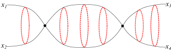
Moreover, in a specific double scaling limit proposed in Gurdogan:2015csr , combining weak coupling with strong imaginary -twists, the -deformed SYM drastically simplifies and gives rise to a family of chiral non-unitary CFTs with 3 effective couplings describing the scalar and Yukawa interactions of three complex scalars and three fermions. Its spectrum of anomalous dimensions, scalar and fermion amplitudes have been studied in a series of papers Gurdogan:2015csr ; Caetano:2016ydc ; Grabner:2017pgm ; Gromov:2017cja ; Chicherin:2017cns ; Chicherin:2017frs . In the particular, single coupling version of these models, the bi-scalar “fishnet” CFT, studied in this paper, the four-point correlation function of certain protected operators was computed in Grabner:2017pgm , providing a rich non-perturbative OPE data for the exchange operators with an arbitrary spin. These results have been generalized to any dimension in Kazakov:2018qbr , where the -dimensional version of the bi-scalar model was proposed. In this paper we extend these results to more general correlators. In addition to the wheel graphs we also consider single and double spiral graphs as shown on Fig.1. We also analyse the results at weak and strong coupling.
An important feature of such models is the drastic simplification of their weak coupling expansion, where in many particular cases (when we turn on a single coupling) it is dominated by various kinds of “fishnet” Feynman graphs Caetano:2016ydc . These graphs represent integrable two-dimensional statistical-mechanical systems by themselves Zamolodchikov:1980mb and can be efficiently studied by the quantum spin chain methods and the double-scaled version QSC Gromov:2016rrp ; Gromov:2017cja . In particular, the individual, so called “wheel” multi-loop Feynman graphs can be computed exactly in terms of multiple zeta values (MZV) Gromov:2017cja .
Importantly, the explicit graph-by-graph integrability property in such models sheds some light on the origins of the planar integrability of their “mother”-theory – the SYM, where the perturbation theory is much more complicated and the reasons for integrability are still obscure. In particular, in the bi-scalar CFT discussed in this paper the integrability is manifest due to the explicit integrability of fishnet graphs dominating the perturbation theory in this model Grabner:2017pgm .
1.1 The conformal “fishnet” theory
We will focus in this paper on a particular example of strongly -deformed SYM – the bi-scalar theory Gurdogan:2015csr . At the classical level, the Lagrangian of the bi-scalar theory is given by222In the literature one also uses notations and . We use ‘bar’ for the Hermitian conjugation.
| (1.1) |
where are complex matrix fields and are their hermitian conjugates. The model retains the global symmetry which is a remnant of the gauge symmetry of the original SYM theory. The effective coupling constant is given by the product of the Yang-Mills coupling and the complex deformation parameter. The general deformed SYM theory depends on three deformation parameters . The Lagrangian (1.1) arises in the double scaling limit, and with and fixed. In this limit, all fields except two scalars get decoupled leading to (1.1).
On the quantum level, to make the theory conformal we have to add various double-trace terms with well-tuned couplings Sieg:2016vap ; Fokken:2013aea ; Fokken:2014soa ; Grabner:2017pgm :
| (1.2) |
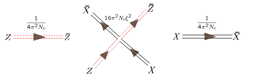
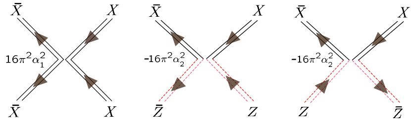
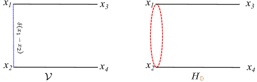
where and are new induced coupling constants and the factor of is introduced for the convenience. The corresponding Feynman rules for all types of double-trace vertices are presented on Fig. 3.
The relative coefficients between the operators in both lines of (1.1) follow from the invariance of (1.1) under the transformations of fields
| (1.3) |
with the conjugate fields transforming accordingly. As we show below, these transformations can be used to establish relations between different correlation functions.
The theory with the Lagrangian is renormalizable. The coupling constants depend on the renormalization scale and the corresponding beta functions have been computed perturbatively in Grabner:2017pgm in the planar limit, for and . Examining zeros of the beta functions, we find that the theory has two fixed points
| (1.4) |
where is given at weak coupling by the following expression
| (1.5) |
Notice that the expansion of runs in powers of with real coefficients.
The planar bi-scalar theory (1.1) possesses a conformal symmetry at the fixed points (1.4) Sieg:2016vap ; Grabner:2017pgm and is integrable Gurdogan:2015csr ; Gromov:2017cja . Viewed as a function of , the relation (1.4) defines two lines of the fixed points. It has been argued in Grabner:2017pgm that the “mother” theory of the bi-scalar model – the deformed SYM – is a nonunitary CFT on a line of (complex) fixed points of double couplings as functions of the ’t Hooft coupling, also integrable in planar limit. It is also natural to expect the existence of such a complex conformal trajectory even at finite .
The bi-scalar ”fishnet” CFT (1.1) is the most studied case of the abovementioned chiral CFTs proposed in [41]. The spectrum of long local operators of the type +permutations, can be efficiently investigated by the asymptotic Bethe ansatz (ABA) equation Caetano:2016ydc – the double scaled version of the Beisert-Staudacher ABA equations for SYM Beisert:2006ez . The short operators of this and other types (also with insertions of derivatives and fields) can be studied by QSC methods Gromov:2017cja and by the quantum non-compact spin chain methods Gurdogan:2015csr ; Gromov:2017cja , when the spins take values on conformal group . The spin-chain approach to this theory is very promising since it would allow us to study there non-perturbative physics starting from the first principals, without any assumptions. Unfortunately, efficient methods of study of non-compact, Heisenberg spin chains are not very well developed, especially for principal series representation in physical space and for higher ranks symmetries, such as , though an important progress has been made in the study of spectral problem for spin chain, in relation with high-energy (Regge) limit of QCD Derkachov:2001yn ; DeVega:2001pu . Another remarkable observation in bi-scalar theory concerns the planar scalar amplitudes: they are dominated by a single multiloop fishnet graph with open boundary and obey a Yangian symmetry, potentially allowing for their computation Chicherin:2017cns ; Chicherin:2017frs . A particular, single-trace four-point correlation function given by such fishnet graph was explicitly computed in Basso:2017jwq 333Their result can be interpreted as a correlator of the form . Alternatively one can interpret it as a leading weak coupling contribution to the point correlator of single trance operators..
We refer to the single trace operators for as -magnon states, in accordance with the ABA description, where the asymptotic anomalous dimension is described by the Bethe state with Bethe roots and conformal spin chain of length . The related Feynman graphs have been described in Caetano:2016ydc . They have a shape of multi-spiral when radial lines of the field coming out of the point where the operator is placed, are “braided” by parallel spirals, as shown on the Fig.1(in the middle for a single spiral, and on the right for the double spiral).
Correspondingly, the simplest set of non-trivial single trace operators has length and numbers of magnons . In addition, one can also introduce Lorentz spin by inserting light-cone derivatives in the following way: . The most efficient way of studying these operators is to extract their conformal data from the OPE of -point functions. Accordingly, we will analyze the -point functions of different topologies, corresponding to the number of the magnons (see Fig.5). The simplest, zero-magnon four-point correlation function was computed to all orders of weak-coupling expansion in Grabner:2017pgm . It is dominated by the wheel graphs containing only two “spikes”. It was shown in Grabner:2017pgm that this quantity has correct conformal properties in the perturbation theory only if one takes into account the double-trace interactions.
In the current paper, we will review the findings of Grabner:2017pgm and continue to study the properties of the four-point correlation functions. In addition, we compute a few related four point-functions of short local operators, corresponding to one- and two-magnon cases. These three types of four-point functions are distinguished by the relative simplicity: for their computation one does not need to appeal to the integrability – the conformal symmetry is enough for this purpose. We then use the obtained results for the four point correlation functions to extract explicit expressions for the anomalous dimensions and structure constants.
All these results represent a unique opportunity of study properties of bi-scalar CFT, in the hope to better understand the non-perturbative structure of non-supersymmetric CFTs in dimensions. They provide rich data for the future integrability based calculations of the correlation functions.
1.2 Correlation functions and their perturbative structure
In this paper, we exploit conformal symmetry to find exact expressions for correlation functions of local protected dimension–two operators
| (1.6) |
as well as of bi-local operators of a “one-magnon” type
| (1.7) |
The reason for the choice (1.2) is that, in the planar limit, the two-point correlation functions of operators (1.2) are protected at the fixed points (1.4)
| (1.8) |
where the normalization factor comes from free scalar propagator.
The pair correlation function of bi-local operators of the type (1.7) defined below as type will represent another type of four-point functions, having one-magnon exchange states in OPE, dominated by single-spiral graphs of the type shown in Fig. 1.
In what follows we consider the simplest unprotected four-point correlation functions of the local operators (1.2), of the following two types:
-
•
Type A
(1.9) -
•
Type B
(1.10) The remaining four-point correlation functions of the operators (1.2) vanish due to nonzero total charge. Notice that type correlation function expansion in small limit is saturated by the two-magnon operators. Two such spin-zero operators, and , are not protected and mix with each other, in such a way that their dimensions are related by the change . The analogous operator in SYM theory is Konishi operator , where as the second operator with the same -charge, , is protected444This combination is obtained by acting on the -BPS operator with lowering operator..
-
•
Type C
We will also define the type-C four-point functions containing one-magnon exchange states:
(1.11) We can also define a similar pair of correlation functions
(1.12) which, due to the relations (1.3), coincide with and , respectively.
-
•
Type D
In addition to (1.9) and (• ‣ 1.2), we also consider a four-point correlation function of scalar fields computed in Grabner:2017pgm
(1.13) As will become clear in a moment, its calculation is closely related to that of given by (1.9) (see (2.9) below). The function is obtained from by Wick contracting two pairs of and fields.
At the fixed point (1.4), the correlation functions (1.9), (• ‣ 1.2) and (1.13) are finite functions of the coupling . The correlation functions (• ‣ 1.2) are related to each other through the first of transformations (1.3) and, therefore, they coincide
| (1.14) |
For the correlation function (1.9), the relations (1.3) imply that should be invariant under the exchange of points
| (1.15) |
A remarkable feature of all considered correlation functions is their iterative structure: the (non-zero) contribution at each successive order of perturbation theory can be obtained from the previous one by action on it by some graph generating integral operators. Thus the relevant graphs have a chain structure and they can be studied using the Bethe-Salpeter equation. In addition, the emerging graph generating operators commute with the generators of the conformal group and their eigenspectrum can be easily found with a help of the conformal symmetry. Thanks to these features the above mentioned correlation functions of the bi-scalar model are explicitly computable in a relatively simple way.
2 Relation to skeleton scalar graphs
In this section, we will describe the structure of Feynman graphs for all types of the studied 4-point correlation functions. We express these correlators in terms of the basic generating functions of the wheel graphs (), single () and double spiral graphs () as on Fig.5. In the section 4 we evaluate these types of the graphs by the Bethe-Salpeter method, by diagonalizing their graph generating kernels. Consequently, we compute all the related structure constants defining the full explicit OPE representation of each of these 4-point functions (• ‣ 1.2)–(1.13).
We will first discuss the connected and disconnected parts of all these 4-point functions and then study the connected planar part of each of them. For the sake of explicitness, we will restrict our discussion to dimensions, but the final formulas will be readily generalized in section 9 to any .
2.1 Connected part of the correlation functions
The four-point correlation functions of the types and (1.9) – (• ‣ 1.2) receive both connected and disconnected (in the sense of factorisation of the coordinate dependence) contributions . The former are suppressed with respect to the latter by a power of
| (2.1) |
but all the most interesting physics resides of course in the connected part. The disconnected contribution is given by the product of two-point correlation functions (1.8) leading to
| (2.2) |
For the correlation function of type and the disconnected contribution is
| (2.3) |
Due to the color structure of bi-local operators in the definition of and , the disconnected part in both cases is of the same order in as the connected part.
Finally, the disconnected part of the correlation function of type is suppressed by the factor of as compared with its connected part.
2.2 Relation of 4-point functions of all types to basic fishnet graphs
The computation of all above-mentioned types of 4-point functions can be reduced to the evaluating Feynman graphs having 3 basic structures of fishnet graphs. They are depicted on the Fig.1 and they are distinguished by the the magnon numbers - - the number of propagating “particles” (dotted spirals lines on the Fig.1) in the exchange channel. We will denote the related generating functions as , and and call them the -magnon functions. As we will see shortly, the Feynman graphs for these functions are computable by the Bethe-Salpeter approach, due to their periodic fishnet structure and conformal properties.
To be more precise, we will define -magnon functions as perturbative expansion w.r.t. the coupling as follows.
For zero-magnon case (the “wheels”) we have
| (2.4) |
where denotes the Feynman graph depicted on the left of Figs.1 and 5 and having interaction vertices (black dots).
For one-magnon case (“spiral”, or “spiderweb” graphs) the structure function looks as
| (2.5) |
where denotes the Feynman graph depicted in the middle of Figs.1 and 5 and having interaction vertices (black dots).
Each graph takes a shape of a spiral consisting of propagators of type wounding around two lines of propagators of type .
Note that we have two distinguished structures depending on the parity of expansion term w.r.t. : for even powers of the spiral on Fig.1 starts and ends on the same (black) line of -propagators, whether as for odd
powers of it starts and ends on different -lines.
For two-magnon case (“double spiral”) we have the structure function
| (2.6) |
where denotes the Feynman graph depicted on the right of Figs.1 and 5 and having interaction vertices (black dots).
Let us relate the correlation functions , , and to , and .
2.2.1 Relations between correlation functions and -magnon functions
First, we can immediately see from Figs. 1(left) and 5(left) and from the definitions (1.13) and (2.4) that
| (2.7) |
Further on, the correlation function is given by the following linear combination of the functions
| (2.8) |
where the last term takes care of double counting of the tree-level diagram in the first terms. It is straightforward to verify that the linear combination on the right-hand side of (2.2.1) satisfies the symmetry relation (1.15).
Comparing (2.2.1) and (2.7) we notice that the two correlation functions are related to each other as
| (2.9) |
Having determined , we can apply (2.7) and (2.2.1) to find the correlation functions and .
For the one-magnon correlation functions we get the following expressions through the even and odd in parts of the magnon function :
| (2.10) |
Finally, the two-magnon correlation function (• ‣ 1.2) coincides with the two-magnon function (2.6):
| (2.11) |
In the next section we review the general method for computing the magnon functions , and based on the Bethe-Salpeter equation and conformal symmetry. The explicit expressions for these functions are derived in section 4.
3 Conformal symmetry and Bethe-Salpeter equations: generalities
As we saw above and discuss in detail in the next section, the correlation functions introduced in previous sections are given by very specific type of fishnet graphs: in each graph the periodically repeating configurations of propagators are connected by pairs of coordinates of the related vertices (see Fig. 5). Each graph can be cut into two disconnected parts by splitting only two vertices. The three cases we are going to consider differ, in particular, by the values of dimensions of four external (protected) operators. For all correlation functions under considerations we have and .
This section is based on the observation that three topologically distinct configurations , and can be written, each, in terms of a suitable “graph-building” operator . In each case we find at the level of the operators
| (3.1) |
where is a nonnegative integer, the constant is proportional to a fixed power of the coupling constant (specified below for each case) and is the dimension of the space-time. In most of the paper we set although, as we will see in the section 9, most of the equations discussed here have a natural generalization to general , where the bi-scalar theory can be also formulated Kazakov:2018qbr . The operators and are represented by the corresponding integration kernels, e.g.
| (3.2) |
in such a way that
| (3.3) |
The problem of finding can be split into two main steps. First, we have to solve the eigenvalue problem for and, then, decompose over the complete basis of the eigenfunctions of .
Fortunately, the first step is simple in our case. The eigenfunctions of which are defined by
| (3.4) |
where and parameterise the eigenstates, are totally symmetric traceless tensors in -dimensional indices . The form of is completely fixed by the conformal symmetry – if the operator commutes with the generators of the conformal group, its eigenstates should transform covariantly under conformal transformations acting on . As such, can be represented as a conformal “triangle” – three-point correlation function of two scalar operators at the points and some reference operator with dimension and spin at the point . Explicitly
| (3.5) |
where 555Following the standard conventions, we shall refer to at zero value of the coupling constant as twist. and . In order to simplify tensor structure, we projected all Lorentz indices onto a light-like vector . In the next section we verify explicitly that the functions (3) diagonalize the graph-building Hamiltonians and find the corresponding eigenvalues .
The scaling dimension in (3) is given by Tod:1977harm
| (3.6) |
where is real nonnegative. For such values of the functions define the complete orthonormal basis of states on the Hilbert space on which the graph building kernel acts. Viewed as a function of , belongs to the irreducible principle series representation of the conformal group labelled by real and nonnegative integer Lorentz spin . Together with (3.4) this leads to
| (3.7) |
where is the normalization factor defined in (A.4) and we used that . The values of in (3.7) can be restricted to be since the states and belong to the same representation and are related to each other through intertwining relation.
Inserting (3.7) into (3.1) we get the following expression for the correlation function
| (3.8) |
The integral over can be evaluated explicitly in terms of four-dimensional conformal blocks Dolan2011 ; Dolan:2000ut ; Tod:1977harm
| (3.9) | |||
the expression in the brackets depends only on the cross ratios and defined as
| (3.10) |
where and are auxiliary complex variables. The conformal block depends on and and it is given explicitly in terms of the hypergeometric functions in (A.1). The coefficient is a ratio of the normalisation coefficients defined in (A.4) and (A.6).
Combining together (3.8) and (3.9) we obtain666The constant should not be confused with the function .
| (3.11) |
where admits the following representation
| (3.12) |
where . Here we combined the two terms on the right-hand side of (3.9) to extend the integration over to the whole real axis and used the identity . Note that doing so we required that
| (3.13) |
This property follows from the fact that the states with the same Lorentz spin and the scaling dimensions and belong to the same representation of the conformal group. We will check (3.13) explicitly in each case.
To bring the integral (3.12) to the standard OPE form we examine the short distance limit , or equivalently and . In this limit, the conformal block scales as and decays exponentially fast for . This allows us to close the integration contour in (3.12) to the lower half-plane and compute the integral on the right-hand side of (3.12) by residues. In terms of the OPE, the condition is equivalent to the restriction on the scaling dimension of exchanged operators.
The integrand in (3.12) has ‘physical’ poles coming from zeros of the denominator
| (3.14) |
and two series of ‘spurious’ poles generated by the kinematical factor and the conformal block . We show in Appendix B that the spurious poles cancel against each other provided that satisfies the following relation
| (3.15) |
with defined in (B.1). Then, the correlation function (3.12) is given by the sum of residues at the physical poles (3.14). Finally, we obtain the following conformal partial wave expansion of the correlation function (3.12)
| (3.16) |
where the OPE coefficients are given by the residues at the physical poles
| (3.17) |
4 Four-point correlators and the conformal OPE data
In this section, we describe Feynman graphs for the types of 4-point correlation functions depicted on Fig.5, and establish the corresponding graph-building operators . In the previous section, it was shown that the eigenvalue of these operators is the only input needed in order to write a representation of OPE type for the correlation function. We diagonalize the operators and present explicit expressions for the conformal data (scaling dimensions and the OPE coefficients) for each of these 4-point functions.
4.1 Zero-magnon case and the wheel-graphs ()
The zero-magnon correlation function was studied in detail in Grabner:2017pgm . Here we re-derive the results of Grabner:2017pgm and show how they fit into the general scheme described in the previous section.
As we show below, the zero-magnon case corresponds to the situation when the correlation function (3.16) receives contribution from magnon-free operators of the type and 777Interestingly, in our case only single box can appear. In space-time dimension this is not the case.. We will see that only these two types of operators with arbitrary spin contribute.
To find the zero-magnon correlation function we have to summed up diagrams shown on Figure 5(left). These diagrams contain an arbitrary number of wheels attached to the rest of the diagram at two (single-trace) vertices. It is easy to see that the integral over the position of these vertices develops a ultraviolet (UV) divergence at short distances. This seems to be in contradiction with expected UV finiteness of four-point correlation function of protected operators. We recall however that quantum corrections induce new double-trace interaction terms (1.1). In particular, the double-trace coupling affects the zero-magnon correlation function. It produces a UV divergent contribution which cancels against that of the wheel graphs in such a way that the four-point correlation function remains UV finite at any order in the weak coupling expansion. Due to form of the double-trace interaction term , it can only affect the contribution of partial waves to (3.16) with zero Lorentz spin . We therefore expect that the contribution of the wheel graphs to (3.16) is well-defined for whereas for the additional contribution due to double traces should be taken into account. We discuss this issue in more detail in Sec.5.
In this section we proceed without taking the double trace interaction into account and identify the contrubution of wheels graphs to (3.16). We will see that the double trace contributions will be automatically taken into account by correct treatment of the singularity at in the forthcoming formulas. We start with constructing the graph building operator and identifying the parameters , and introduced in (3.1). We recall that the parameters define the scaling dimension of the external operators. Since the wheel graphs have only one propagator attached to each external leg we have .
To first two orders of the weak coupling expansion the zero magnon function is given by the sum of diagrams shown in Fig.6. The expressions corresponding to the first two diagrams are
| (4.1) |
where each scalar propagator brings in the factor of . These expressions can be represented as st and nd powers of the following graph building operator
| (4.2) |
Indeed, we verify that
| (4.3) |
from where it is clear that for a general graph with wheels we get . It is straightforward to verify that the function (4.2) transforms covariantly under the conformal transformations acting on .888The simplest way to check this is to employ inversions and take into account that . As a consequence, the corresponding integral operator commutes with the generators of the conformal group.
Thus the zero-magnon correlation function can be written as
| (4.4) |
Comparing with the general expression (3.1) we deduce that and in the zero-magnon case.
4.1.1 Eigenvalue of the zero-magnon graph-building operator
In order to use the general expression for the correlation function (3.16), we have to determine the eigenspectrum of the graph building operator (4.2). In virtue of conformal symmetry, its eigenstates are given in (3) with and . Substitution of (4.2) into (3.4) leads to an integral, which can be evaluated using the star-triangle identity as explained in appendix C.2. Going through the calculation we obtain the following simple result Grabner:2017pgm
| (4.5) |
It is easy to see that is invariant under , in agreement with (3.13). We can also check that (4.5) verifies the relation (3.15) that ensures the cancellation of spurious poles. In the present case, for , it follows from (B.1) that for integer and thus (3.15) reduces to
| (4.6) |
which is indeed satisfied for (4.5).
4.1.2 Spectrum for zero-magnon exchange operators
We can now use (4.5) to determine the scaling dimension of the zero-magnon operators contributing to the correlation function (3.16). Substituting (4.5) into the relation (3.14) and replacing we find that the scaling dimensions satisfy the following quartic equation
| (4.7) |
subject to the additional condition . At finite coupling, this yields the following expressions for the scaling dimensions
| (4.8) |
The two remaining solutions to (4.7) are related to (4.1.2) by and describe shadow operators with .
At weak coupling, for , and nonzero Lorentz spin, , the scaling dimensions (4.1.2) look as
| (4.9) |
and the corresponding operators can be identified as twist-2 and twist-4 operators, respectively. 999This explains the meaning of the subscript of . They have the following form and where dots denote similar terms with light-cone derivatives distributed between the fields. Similarly to Gromov:2017cja , the twist operators can be written, due to the equations of motion, as .
Notice that the weak coupling expansion of (4.1.2) goes in powers of which is exactly what one expects since each wheel in the graph shown in Fig. 5(left) is attached to the rest of the diagram through two single-trace vertices. Something special happens at . In this case, we find from (4.1.2)
| (4.10) |
and the weak coupling expansion looks as
| (4.11) |
Surprisingly, for the weak coupling expansion of the scaling dimension starts from the power , instead of the naively expected (the power corresponding to each insertion of the graph-building operator (4.2)).
To understand the reason for this we examine the eigenvalue of the zero-magnon kernel (4.5) for and
| (4.12) |
We notice that it goes to infinity at small . Then, expanding (4.4) in powers of we find that the contribution of the states with to the correlation function at order is proportional to and it diverges for . This is in agreement with our expectations that the contribution of the wheel graphs is well defined for all states except those with . To remove the divergence we have to include the contribution of double traces.
We observe that, in the resummed expression for the correlation function (4.4), the contribution of the states with to involves the integral which is convergent for at finite (for the integral to be well-defined we assume that has a small imaginary part). It is easy to see that, at weak coupling, the integration over small produces a square-root singularity at the origin, . This explains why the weak coupling expansion of in powers of is divergent. At the same time, this also suggests that the double-trace contribution should be essential only in the weak coupling regime whereas at finite coupling it can be safely ignored. We discuss this issue in more detail in Sect. 5.
Arriving at (3.16) we have tacitly assumed that the physical poles (3.14) are located away from real axis in (3.12). As follows from (4.7), at weak coupling, the two physical poles located at pinch the integration contour at the origin for and produce a divergent contribution. The role of the double-trace contribution is to subtract this divergence and, thus, make the weak coupling expansion of well defined. Turning the logic around, we can say that the double traces provide a nonvanishing contribution to the scaling dimensions because the eigenvalue (4.5) diverges as for . The relation (4.10) is in a perfect agreement with the result of explicit loop calculation Grabner:2017pgm .
We recall that the correlation function (3.16) is given by the sum over the solutions to (3.14) with . In our present case for the solution (4.10) satisfy for real . As was mentioned above, for the correlation function (3.16) to be well-defined should have a nonvanishing imaginary part (see Appendix D for discussion of analytical properties of (3.16)). The expression (4.10) satisfies for . For , the scaling dimension is given by the same expression (4.10) upon replacing .
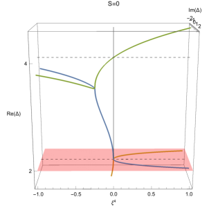
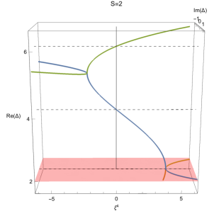
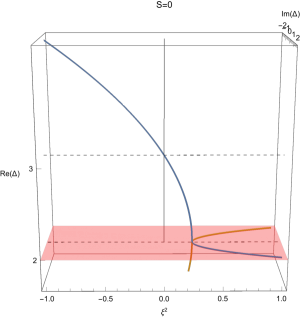
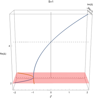
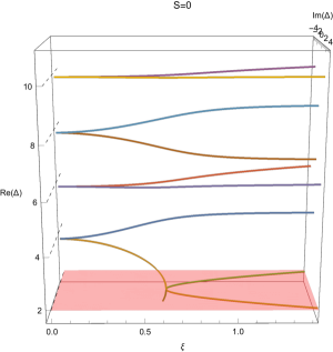
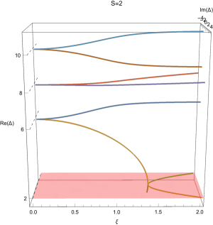
Let us examine the properties of the scaling dimensions (4.1.2). The dependence of and on is shown on Fig. 7 for and . We observe that the two functions (4.1.2) represent in fact two branches of the same analytic function. It has two branch points located at
| (4.13) |
For the two operators collide, , whereas for one of the operators collides with its shadow, . 101010If the theory were unitary, the scaling dimensions and would respect the Neumann-Wigner non-crossing rule and remain to be different from each other for any coupling Korchemsky:2015cyx . The collision of operators at modifies analytic properties of the correlation function . According to (D.2), the correlation function has the cut for that starts at . It is easy to see from (4.5) that is a decreasing positive-definite function of . Therefore, the cut starts at (corresponding to ) and goes to infinity along real axis. In the vicinity of the branch point, it follows from (4.7) that for leading to Korchemsky:2015cyx .
Strong coupling.
At strong coupling, for , the relation (4.7) has four solutions (with ). Among them only two satisfy the additional condition . The corresponding expressions for the scaling dimensions are
| (4.14) |
where integer satisfies the condition and depends on .
4.1.3 Structure constants for zero-magnon exchange operators
We apply the general relation (3.17) to find the OPE coefficient for zero-magnon operators Grabner:2017pgm
| (4.15) |
Stricktly speaking, is given by the product of (properly normalized) point correlation functions and . In unitary CFT they are complex conjugated to each other and, as a consequence, is positive definite. This is not the case for the conformal fishnet theory (1.1) and (1.1). In virtue of the symmetry (1.3) the above mentioned 3-point functions coincide and, therefore, is given by the square of the 3-point correlation function of two protected and one unprotected operators
| (4.16) |
We will generalize this result to a more complicated structure constant involving two non-protected operators in section 8.
Weak coupling limit.
Replacing the scaling dimensions in (4.15) by their expressions (4.1.2) we can obtain the OPE coefficients at weak coupling.
First, consider twist-2 operators with the scaling dimension and non-zero spin . In this case we get
| (4.17) |
where is the Euler polygamma-function. Notice that becomes singular for . Similar to the situation with the scaling dimension , this happens because the two limits and do not commute. To get the correct result for at weak coupling, we should first put in (4.15) and, then, expand it in powers of . This gives
| (4.18) |
In analogy with (4.11), the weak coupling expansion starts at order indicating that is sensitive to the contribution of the double traces.
For twist operators we find from (4.15) and (4.1.2)
| (4.19) |
In distinction with (4.18), the weak coupling expansion of starts at order and runs in powers of . The latter property is in agreement with our expectations that twist operators are not affected by double-trace interaction. The twist-4 OPE coefficient (4.19) is suppressed by the factor of as compared with (4.18). Due to the equation of motion, , the corresponding operator takes the form . The reason for the above-mentioned suppression is that and leading to .
Strong coupling limit.
At strong coupling the dimension become large according to (4.14) and we get
| (4.20) |
Thus we see that the structure constant at strong coupling is exponentially small since .
4.1.4 Zero-magnon 4-point correlation function
Having determined the conformal data of the zero-magnon operators, we can apply (3.11) and (3.16) to compute the four-point correlation function (3.11) and (3.16)
| (4.21) |
where we replace the scaling dimensions of the external protected operators by their values, , and the function is given by
| (4.22) |
where the sum runs over the states with the scaling dimension (4.1.2) and the OPE coefficients (4.15). Here is the four-dimensional conformal block defined in (A.1) (with ).
The relation (4.22) involves an infinite sum over the conformal blocks and it is not obvious a priori that one can find a closed expression for even at weak coupling. We show in section 5 by explicit two-loop calculation that can be expressed in terms of special functions, the so-called harmonic polylogarithms (HPL). In section 6 we extend this result to any order of the weak coupling expansion. Also in section 7 we analyse the strong coupling limit of the expression (4.22). The analytic properties of with respect to the coupling are discussed in Appendix D.
According to (2.7) and (2.2.1), the correlation functions and are given by a linear combination of the zero-magnon functions symmetrized in . Let us see what effect the exchange of and has on the function . As follows from (3.10), the cross-ratios transform under the exchange of with as and . The corresponding transformation of the conformal blocks looks as
| (4.23) |
This relation follows from (3.9), it can also be verified directly from the definition (A.1). Combining together (4.22) and (4.23) we conclude that, in the expressions for and the terms in (4.22) with odd cancel out whereas those with even get doubled.
4.2 One-magnon case and single spiral graphs ()
In this subsection, we consider the one-magnon correlation function described by graphs shown in Fig. 5(middle). As we will see shortly, its calculation is simpler than that of and . Since the graph contributing to have two propagators attached to and and only one to and , we identify the scaling dimensions at the external points as
| (4.24) |
To identify the graph-building operator , we consider the first few terms in the weak coupling expansion of (see Fig.8). The expressions corresponding to the first two diagrams are
| (4.25) |
Let us show that these expressions can be represented as and power of the graph building operator with the integral kernel
| (4.26) |
Indeed, we apply (3.3) to get
| (4.27) |
It is clear from these examples that, in general, . Thus the correlation function can be written as
| (4.28) |
Comparing with the general form (3.1) we see that and .
4.2.1 Eigenvalue of the one-magnon graph-building operator
As in the previous case, we can verify that the integral operator with kernel given by (4.26) commutes with the generators of the conformal group acting on the external points and the corresponding conformal weights given by (4.24). As a consequence, its eigenstates are given by (3) with and . The eigenvalue equation (3.4) reduces to an integral which can be evaluated using the star-triangle identity, as explained in Appendix C.3. The result turns out to be quite simple
| (4.29) |
It is obviously invariant under and satisfies (3.13). We can use (4.29) to verify the condition (3.15). In the present case, for and , we find from (B.1) that for integer so that the relation (3.15) takes the form
| (4.30) |
where . It is easy to see that it holds indeed. 111111Note that the factor in the expression for plays an important role for this equation to be satisfied.
4.2.2 Spectrum of one-magnon exchange operators
Substituting (4.29) into (3.14) and taking into account that , we determine the scaling dimension of the one-magnon operators contributing to the correlation function (3.16)
| (4.31) |
For we have
| (4.32) |
Interestingly, this expression coincides with the asymptotic dispersion relation for the one-magnon state previously found from the double-scaling limit of asymptotic Bethe ansatz (ABA) in Ref. Caetano:2016ydc . Following the ABA approach, one could have expected that the asymptotic dispersion relation (4.32) should be corrected already at order by the wrapping corrections. The relation (4.32) implies that the wrapping corrections to the one-magnon operator vanish. This is indeed the case for the single wrapping contribution found in Caetano:2016ydc . The relation (4.32) is indeed consistent with the ABA, including the known single wrapping correction!
Weak coupling.
At weak coupling, the scaling dimension (4.31) of the one-magnon states reads
| (4.33) |
Strong coupling.
4.2.3 Structure constants with one-magnon exchange operators
We can also employ the general equation (3.17) to find the OPE coefficient
| (4.35) |
As in the previous case, it is given by the square of the point function of two protected and one unprotected operator, .
Weak coupling.
At weak coupling, we obtain from (4.35) and (4.33)
| (4.36) |
In particular for we find
| (4.37) |
Since the first few coefficients do not involve wrapping it should be possible to compare with the perturbative ABA based general expressions from Escobedo2010 ; Gromov2012 .
Strong coupling.
4.2.4 One-magnon four-point correlation function
Substituting (4.24) into (3.11) and (3.16), we obtain the one-magnon 4-point correlation function
| (4.39) |
where
| (4.40) |
and the sum runs over the states with the scaling dimensions and the OPE coefficients given by (4.31) and (4.35), respectively. Notice that in the above sum there is only one state for each value of the spin and spin takes all non-negative integer values. In section 6 we study (4.40) at weak coupling and compare it with the result of perturbative calculation performed in section 5. Also in section 7 we analyse the strong coupling limit of (4.40).
4.3 Two-magnon case and double-spiral graphs ()
The two-magnon correlation function is given by graphs shown in Fig. 5(right). Since these graphs have two propagators attached to all four external points, we identify the scaling dimensions as
| (4.41) |
As before, in order to construct the graph building operator for the two-magnon case , we examine the first few orders of the weak coupling expansion of (see Fig.10). The expressions corresponding to the first two diagrams on Fig.10 are
| (4.42) |
Note that the two-loop integral entering factorizes into a product of one-loop integrals. This is not the case already at the next order for the right-most diagram in Fig.10.
The kernel generating the two-magnon diagrams is
| (4.43) |
Indeed we verify that the convolution of reproduces all the diagrams depicted in Fig.10.
| (4.44) |
Thus for the sum of all two-magnon diagrams we get
| (4.45) |
Comparison with the general expression (3.1) shows that and .
4.3.1 Eigenvalue of the graph-building operator
To compute the two-magnon correlation function (4.45) we have to diagonalize the operator . We can use (4.43) to show that it commutes with the generators of the conformal group. As a consequence, its eigenstates are given by (3) with . To find the corresponding eigenvalue , we replace the eigenstates in (3.4) by their explicit expressions (3). This leads to a rather complicated integral on the left-hand side of (3.4). We can simply its calculation by sending on the both sides of (3.4). In addition, we project all Lorentz indices on an auxiliary light-like vector (with ) and obtain the following representation for
| (4.46) |
where and we put for convenience.
4.3.2 Spectrum
The scaling dimensions of the two-magnon operators satisfy the relation
| (4.49) |
subject to and being even nonnegative.
This time the spectrum of ’s has a rich structure since for each value of there are infinitely many solutions to (4.49). Indeed, as follows from the first relation in (4.3.1), the function (4.3.1) has an infinite sequence of double poles at for . As a consequence, for small the relation (4.49) always has two solutions in the vicinity of describing operators with twist and even spin . 121212Like in the case of due to the symmetry of the correlation function under the exchange of points and only even spins contribute to . Indeed we see on Fig.12 that all levels are twice degenerate at weak coupling.
The weak coupling expansion of can be found by replacing by its expansion in the vicinity of the pole. Going through the calculation we obtain
| (4.50) |
with the expansion coefficients given by
| (4.51) |
For each and , the relations (4.50) and (4.51) yield two scaling dimensions that are related to each other through the transformation . For even , the expansion coefficients in (4.50) are real. For odd , the leading coefficient is pure imaginary (see Fig.12). The relations (4.50) and (4.51) describe the scaling dimensions of an infinite set of operators, two per each twist and spin .
In particular, for and , for the two-magnon operators of the form the scaling dimensions are given at weak coupling by
| (4.52) |
The first 4 terms reproduce the prediction from ABA Caetano:TBP including the first Lüscher correction.
Critical coupling.
The dependence of the two-magnon scaling dimensions on the coupling constant is shown on Fig.12. As can be seen from this figure, for each the lowest level approaches the value at some finite . Expanding near we find the corresponding value of the coupling constant
| (4.53) |
Numerically, for we obtain131313For comparison, for a different operators with with zero spin of the type we get a very similar behaviour with the critical points at Gromov:2017cja .
| (4.54) |
For , the scaling dimension develops an imaginary part. As we see in a moment, it grows linearly with at strong coupling.
Strong coupling.
Solving (4.49) at strong coupling, we have to identify the values of at which vanishes. A close examination of (4.3.1) shows that has infinitely many zeroes in for any even of . For example, for the first few zeroes of (4.3.1) satisfying can be found numerically as
Notice that the real part of most of the zeros is close to integer. They determine the leading large asymptotics of the scaling dimension of all but two states shown in Fig.12.
4.3.3 OPE coefficients
From (3.17) we get for :
| (4.56) |
where is given by (A.6) for . Replacing with (4.3.1), we obtain a rather cumbersome expression for , we do not present it here.
Weak Coupling.
Expanding the resulting expression for in powers of , we get the OPE coefficients for the operators with twist and Lorentz spin
| (4.57) |
Here is the one-loop anomalous dimension defined in (4.51) and the coefficient is given by
| (4.58) |
Strong Coupling.
To analyse the strong coupling behaviour of (4.56) it is convenient to rewrite it as
| (4.59) |
where we used (4.49) to get rid of . Since for most of the states approaches a constant value at strong coupling, we see from (4.59) that should decay as . For the two remaining states whose imaginary part grows linearly in , the OPE coefficient (4.59) decreases slower as for real . We recall however that in order for the correlation function (3.12) to be well-defined, should have an imaginary part. For with large imaginary part the structure constant of the lowest level at each decays exponentially and thus the OPE expansion at strong coupling should be dominated by the other state, for which at . This is rather different behaviour to that of two other correlators and needs further investigation. We discuss this issue briefly in section 7.
4.3.4 4-point correlation function
Having determined the scaling dimensions and the OPE coefficients we can compute the two-magnon correlation function
| (4.60) |
where
| (4.61) |
We note that for each spin and twist there are two states, as one can see from the weak coupling expansion (4.50).
5 Correlation functions at weak coupling from Feynman diagrams
In the previous sections, we have derived three different types of four-point correlation functions by applying the operatorial methods. Namely, we have solved the underlying Bethe-Salpeter equations by diagonalizing the corresponding “graph-building” kernels with a help of the conformal symmetry. Doing so, we have ignored the double trace counterterms (1.1) which are nessesary for the consistent definition of the bi-scalar model (1.1) on the quantum level and for restoring the conformal symmetry of the theory.
In this section we discuss the role of the double-trace interaction terms (1.1). We show that they are necessary at weak coupling in order to make each order of the perturbation expansion of the correlation functions to be finite. At the same time, they do not affect the results for the correlation functions at finite coupling obtained in the previous section.
Let us review the role of double-trace couplings and from the action (1.1) in perturbative computations of the correlation functions and . Below we discuss which of the topologies of the Feynman graphs , or have to be completed with the double-trace interactions in order to have meaningful weak coupling expansion of the abovementioned four-point functions.
5.1 Double-trace contribution to
We recall that the four-point functions are completely defined, at least for any finite , by the zero-magnon function . The latter is given by sum over the wheel graphs shown in Fig. 1. As was already mentioned, each wheel in these graphs develops a ultraviolet divergence at short distances. We expect that the double-trace contribution should remove this divergence.
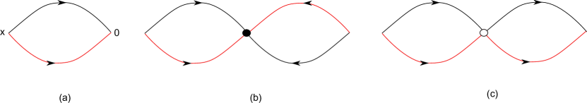
The double-trace interaction is described by the action (1.1). It is easy to see that, due to the cylindrical topology of the underlying planar graphs, among four different double-trace interaction terms in (1.1) only one term can contribute to in the planar limit. It generates a new local quartic scalar vertex. The resulting planar graphs contributing to are shown in Fig.13. They are obtained by gluing together wheel graphs.
Indeed, the insertion of the double-trace vertex effectively splits the planar wheel Feynman graph into two disconnected parts, with the single trace operators, and , attached to each part.
As we demonstrated in the previous section, the wheel graphs can be summed up by introducing the graph building operators . In the similar manner, we can take into account the graphs shown in Fig. 13 by replacing the kernel in the equation (4.22) by a linear combination of operators and generating double-trace vertices and scalar loops, respectively (see Fig. 13). Since the contribution to the correlation function of individual diagram shown in Fig. 13 is divergent, we introduce dimensional regularization with . Then, the regularized operators and are defined as
| (5.1) |
where is a test function. They admit a simple diagrammatic representation, see Fig. 14(right) and (left), respectively. We would like to emphasize that the operators (5.1) are well-defined for .
Making use of the operators (5.1) we obtain the following representation for the zero-magnon correlation function
| (5.2) |
where is the double-trace coupling at the fixed point (1.4).
Expanding (5.2) in powers of the couplings and we find that the first few terms of the weak-coupling expansion of are given by graphs depicted in Fig. 16 below. We compute them later in this section. It is easy to see that higher order terms of the weak-coupling expansion of (5.2) produce graphs shown in Fig. 13.
Note that for the conformal symmetry of the correlation function (5.2) is broken. To elucidate the mechanism of restoration of the conformal symmetry of and the role played by the double traces, we present below the two-loop calculation of the correlation function (5.2).
Applying the identity as , we find from (5.1) that . This means that the operator is singular on the space of functions that do not vanish at short distances . Examining the expression for the eigenfunctions (3), we find they scale at short distances as for and . We recall that computing the correlation functions in the previous section we deformed the integration contour over into the lower half-plane. It is easy to see that in this case vanishes for and, as a consequence, the operator does not develop UV divergences. Moreover, as follows from the definition (5.1), the double-trace operator annihilates the eigenstates with and, therefore, does not contribute. This explains why the double-trace interaction can be neglected when computing the four-point function by the Bethe-Salpeter method. The appearance of UV divergences at weak coupling is a manifestation of analytic properties of . As a function of , it has a square-root cut at the origin so that its pertubative expansion runs in powers of . We have already observed this phenomenon on the example of the scaling dimension (4.11).
5.2 Double-trace contributions to and

The inspection of Feynman graphs defining and shows that the double-trace interactions with the coupling do not contribute in the planar limit. On the other hand, the interactions with the double-trace coupling do contribute to both correlation functions through the graphs of the type shown on Fig.15 on the example of . Each vertex depicted by white blobes on Fig.15 describes both single- and double-trace couplings. The contribution of each such vertex to is UV divergent and it is proportional to . As a result, it vanishes at the fixed point (1.4), so that we are left only with the sums over UV finite single spiral graphs summed up by the UV finite structure function . This property is not surprising given the fact that the correlation function has to be a finite function of whereas the Feynman diagram in Fig.15 involves the ultraviolet divergent scalar loops.
The function is regular at and its weak-coupling expansion runs in powers of . The expression for at arbitrary coupling has been derived in section 4.2 using the Bethe-Salpeter equation in the form of conformal partial wave expansion, Eqs. (2.2.1), (4.39) and (4.40).
The correlation function also receives UV divergent contribution from planar graphs similar to those shown in Fig. 15. Their contribution vanishes at the fixed point through the same mechanism as in the previous case. This means that is defined by the two-magnon function , see Eq. (2.11). Since two-magnon graphs contributing to contain even number of single-trace vertices, the weak coupling expansion of runs in powers of . At arbitrary coupling, is given by the conformal partial wave expansion (4.60) and (4.61).
In the rest of this section, we compute the first few terms of the weak coupling expansion of the 4-point correlation functions and, then, compare them with the exact expressions obtained in section 4.
5.3 Type
In the previous sections, was defined in terms of the function by (2.7), and is given by the wheel diagrams shown in Fig.6. As we already discussed, this definition is not complete and has to be supplimented with the double-trace contributions. The reason for this is that each diagram in Fig.6 is UV divergent and the extra double trace contribution is needed to make each term of the weak coupling expansion to be UV finite.
To illustrate this, we examine the first few terms of the weak coupling expansion of . They are given by Feynman diagrams shown in Fig. 16
| (5.3) |
where denotes the contribution of diagram with double-trace vertices and single-trace vertices. We recall that depends on only one double-trace coupling whose value is given by (1.4) at the fixed point.
The first term on the right-hand side of (5.3) has been previously defined in (4.1), . The correction to (5.3) can be computed from Feynman graphs contributing to and is given by a finite four-dimensional “cross” integral (see Fig. 16)
| (5.4) |
where the factor comes from the relation (2.7) between and , is the symmetry factor, and has a simple form when expressed in terms of auxiliary variables defined in (3.10)
| (5.5) |
The function inside the brackets is known as the Bloch-Wigner function.
The two-loop corrections and come from last two Feynman diagrams shown in Fig. 16. The corresponding Feynman integrals are divergent and require regularization. In dimensional regularization with we have
where the notation was introduced for
| (5.6) |
The integral on the right-hand side has a UV divergence coming from integration at short distances . Applying the identity we find that the residue of at the pole is proportional to the same one-loop integral that enters (5.4). The same is true for the function . As a consequence, the divergent part of two loop correction to (5.3) takes the form
| (5.7) |
Since at the fixed point (1.4), UV divergences cancel in the sum the single- and double-trace contributions. We conclude that the two-loop correction to (5.3) is UV finite as it should be.
Going through the calculation of a finite part of the two-loop contribution we find that it factorizes into a product of one-loop correction (5.4) and a logarithm of the cross-ratio
| (5.8) |
Combining this relation with (5.4) and (5.8) we obtain that the correlation function (5.3) takes the expected form (4.21) with the function given at two loops by
| (5.9) |
Here we replaced the double-trace coupling by its value (1.4) at the fixed point .141414This choice is syncronized with the sign convention in (4.10). For , the function is given by the same expression with replaced with .
Notice that the correction to (5.9) comes entirely from the double-trace contribution. In the next section we show that (5.9) is in a perfect agreement with the exact expression for , Eq. (4.22), which was obtained by resumming the wheel graphs shown in Fig. 6. This is in agreement with our expectations that the double-trace contribution to can be ignored at finite coupling.
5.4 Type
The weak coupling expansion of the one-magnon correlation function is defined by Feynman diagrams shown in Fig. 8. The contribution of the first two diagrams is given by (4.2). In distinction from the previous case, the corresponding integrals are well-defined in dimensions and do not require regularization.
In particular, the one-loop correction defined in (4.2) can be expressed in terms of the “cross” integral (5.4)
| (5.10) |
Then, the one-magnon correlation function takes the expected form (4.39) with given at weak coupling by
| (5.11) |
In the next section, we reproduce this expansion from the exact expression (4.40) for and also produce explicit expressions for higher order terms.
5.5 Type
The two-magnon correlation function is defined by Feynman diagrams shown in Fig. 10. Like in the previous case, the corresponding integrals are well-defined in dimensions and do not require regularization.
The weak coupling expansion of runs in powers of and first two terms are given by (4.3). As was mentioned before, the contribution to is given by a two-loop Feynman integral (4.3) that factorizes into the product of one-loop integrals. The latter take the form (5.4) and, as a consequence, it can be expressed in terms of Bloch-Wigner function
| (5.12) |
The resulting expression for the two-magnon correlation function takes the expected form (4.60) with
| (5.13) |
We managed to reproduce both terms of the expansion (5.13) from its expansion over conformal blocks (4.61) by expanding it at weak coupling. For that we followed the procedure explained in the next section 6.
6 Prediction for the 4-point correlation functions at weak coupling from OPE data
In section 4, we determined the conformal data of the operators that appear in the conformal partial wave expansion (3.16) of the correlation functions at finite coupling. This expansion takes the form of double infinite sums over spins and dimensions. It is not obvious a priori that these sums can be evaluated in a closed form. We demonstrate in this section that, at weak coupling, these sums can be computed order by order in perturbation theory. For zero- and one-magnon functions, and , respectively, the result can be written in terms of special class of iterated integrals known as single valued harmonic polylogarithm functions (SVHPL) Brown:2004ugm ; Dixon:2012yy . The two-magnon function has a more complicated form and it can be expressed in terms of elliptic polylogarithms.
6.1 Zero-magnon case (Type )
As we already emphasized before, an interesting fact about is that it receives corrections from the double trace interaction. As a result, its expansion goes in powers of rather than in .
In the previous section we computed the first three terms of the weak-coupling expansion of the function defined in (4.22). Taking into account (5.9) as well as the explicit expression (5.5) for the function , it is natural to look for a general expression for in the form
| (6.1) |
where and are defined in (3.10). The goal of this section is to compute explicitly starting from the OPE expansion (4.22).
Note that the dependence on the coupling constant enters into (4.22) only through the scaling dimensions and given by (4.1.2). For general their weak coupling expansion only involves powers of . We recall however, that, due to non-comutativety of the limits and , for the weak coupling expansion of does contain powers powers. This means that all terms on the right-hand side of (6.1) with odd powers of come entirely from the contribution of the twist-2 operator with zero spin. We would like to emphasize that the scaling dimension of this operator has to satisfy the condition . Together with (4.10), this implies that should have a nonzero imaginary part . For we have to exchange the operator with its shadow whose scaling dimension is given by and it can be obtained from (4.10) through the transformation . This ambiguity exactly corresponds to the ambiguity of choosing the fixed point (1.4). In what follows we assume that and apply (4.10).
In order to find the explicit expressions for the coefficient functions we match (6.1) into the OPE expansion (4.22) in the short distance limit, and , or equivalently . In this limit, the conformal blocks scale as and their expansion in powers of the coupling generates terms of the form with not exceeding the order in the coupling. The small expansion of involves the same terms and their coefficients can be computed for any finite using the exact expressions for the conformal data of the operators.
A nontrivial property of is that for they can be expanded over the basis of special iterated integrals, the so-called harmonic polylogarithms (HPL) (see Remiddi:1999ew ; Maitre:2005uu ), schematically
| (6.2) |
where the sum runs over the two sets of indices (including empty sets) and with and taking the values . Most importantly, the number of terms on the right-hand side of (6.1) is finite for any thus allowing us to find the expansion coefficients by matching the small expansion of into the corresponding expansion of the basis of HPL functions. Namely, comparing the coefficients in front of terms on the both sides of (6.2) with sufficiently large we obtain an overdetermined system of linear equations for . It is remarkable that for any finite this system has a unique solution.
For the first few coefficient functions we find
| (6.3) |
where we introduced a short-hand notation for and .
The same expressions can be rewritten in terms of classical (di)logarithm functions
as
| (6.4) |
We verify that these expressions coincide with the result of the two-loop calculation (5.9).
It is convenient to assign to each term on the right-hand side of (6.2) and (6.1) the weight equal to the total length of the sets . Then, is given by a linear combination of weight functions whereas expansion of contains both weight and weight functions. We see that the maximal weight of increases by one at each loop order. Correspondingly, the dimension of the basis of the functions increases rapidly at higher loops. The number of terms in the expression for at loops is given by:
| loops | 3 | 4 | 5 | 6 | 7 |
|---|---|---|---|---|---|
| dimension | 38 | 48 | 154 | 244 | 508 |
The resulting expressions for in terms of HPLs are rather lengthy and we do not present them here.
The coefficient functions should be single-valued functions of for . This property is not obvious from (6.2) since HPL functions have, in general, branch cuts that start at and . We can use this information to restrict the basis of possible functions. The HPLs can enter (6.1) through special linear combinations which are free from the branch cuts. They are known as single-valued harmonic polylogarithms , their definition can be found in Brown:2004ugm ; Dixon:2012yy . The resulting expressions for in terms of SVHPLs are 151515We attach to the arXiv submission an auxilary file containing the expressions for SVHPLs of the weight up to in terms of the HPLs.
| (6.5) | |||||
Similar expressions up to loops can be found in a Mathematica file attached to this submission.
6.2 One-magnon case (Type )
Going along the same lines as in the previous case, we were able to expand the sum (4.40) in terms of the SVHPLs. The weak-coupling result (5.11) suggests to look for in the form
| (6.6) |
The explicit expressions for the first few coefficient functions are
| (6.7) |
We verify that the first two terms reproduce correctly the perturbation theory result (5.11).
6.3 Two-magnon case (Type )
In this case we only managed to reproduce the tree level and -loop perturbation theory result (5.13). We found that it is not possilbe to express the -loop expression in terms of SVHPLs. We found that it is given by elliptic function. In small limit the underlying elliptic curve degenerates and the correlator can be written in terms of HPL’s of multiplied by powers and logarithms of . 161616We would like to thank F. Aprile, J. Bourjaily, J. Drummond, P. Heslop and O. Gurdogan for very useful discussion on related issue.
7 Classical (Strong Coupling) Limit of the 4-point Correlators
In this section, we investigate the strong coupling limit of the 4-point correlators. Even though the world-sheet description of this theory is still not known, it was shown in Gromov:2017cja that there is a classical limit of the underlying integrability construction for the spectrum where it reduces to an algebraic curve reminiscent of that of the classical strings in in the full theory. Similarly, we will see that the leading strong coupling asymptotics of the correlation function is saturated by one state with large and the corresponding result scales as , where is a certain function of cross-ratios. Moreover, since this classical asymptotics reminds the behavior of the three point correlation functions for short operators in strongly coupled SYM theory in planar limit (see for example Gromov:2011jh ; Kazama:2012is ). Whereas it would be premature to conclude that this points to the dual string description for the bi-scalar model, the observed behaviour looks very much like an action evaluated on some classical solution. All that constitutes an evidence towards existence of the classical limit of the fishnet theory at strong coupling . The possible relation to the recently proposed AdS sigma model description of the ground state of the fishnet theory for infinite by Basso:2018agi is also yet to be understood. In this section we assume that takes a generic value in the range 171717As below we find square roots and logariphms for definiteness we also assume in the calculation that .. The convergence is not uniform and the limits or have to be taken with extra care. We also assume that where is large and real and is a small positive phase. This assumption is necessary as the correlator has poles at real values of which accumulate at infinity and the limit is not defined.
7.1 Correlation function for zero-magnon case (wheel-graphs)
First we consider the correlation function . It is obtained from the zero-magnon function given by (4.22) via (2.7). As we discussed above, this results in dropping terms with odd in the sum (4.22) and doubling the terms with even . In this subsection, we compute (4.22) in the limit when .
Our main assumption, which is backed by intensive numerical analysis, is that for the sum in (4.22) is saturated by large spins . Then, replacing the conformal blocks in (4.22) by their asymptotic behavior at large and , we can evaluate the sum over by the saddle-point method. In what follows we only evaluate the leading exponential factor. The pre-exponent and the subleading terms can be computed by the same method, we leave it to future studies.
Before we begin we notice the following property of the structure constant (4.15)
| (7.1) |
It allows us to write the 4-point function (4.22) in the following way
| (7.2) |
where is given by the hypergeometric function in (A.2). This expression considerably simplifies our analysis as it allows to replace the sum over by an integral with exponential precision at large and the evaluate it by the saddle point method.
The asymptotic behavior of the conformal block can be found by using a series representation of the hypergeometric functions in (A.2)
| (7.3) |
Then rescaling the variables as
| (7.4) |
we expand the expression under the sum at large and extremize in to obtain
| (7.5) |
in agreement with Hogervorst:2013sma .
Similarly we replace the structure constants (4.15) by their leading asymptotic behaviour at large and to get from (7.2) and (2.7)
| (7.6) |
where the sum runs over even spins , both positive and negative. We recall that for each there are only two values of that contribute to the sum, and , given by (4.1.2). At strong coupling, we apply (7.4) to find that they have different dependence on the spin
| (7.7) |
Note that for we get purely imaginary . In order to get a consistent strong coupling limit we should take to have slightly negative phase, so that at strong coupling. After that we substitute (7.4) into (7.6) and extremize the expression in the exponent over to get
| (7.8) |
where the two states (7.7) produce two different exponents
| (7.9) |
where . Notice that is positive whereas is purely imaginary. As a consequence, has a large negative real part and, therefore, the correlation function (7.9) is exponentially suppressed at strong coupling, as it is expected for the tunneling processes in the classical limit.
Let us also point out that the state which saturates the sum over in the sum (7.6) has the following scaling dimension and spin
| (7.10) |
with the upper sign for and lower for . It would be interesting to find a classical model which reproduces these results.181818In analogy with spin chain we expect that to be some variation of the classical Toda spin chain.
As a test of our result we consider the small limit of (7.8). In this limit, we expect that the leading contribution to the correlation function should come from the states with leading to . Expanding the relations (7.9) and (7.1) at small we find
| (7.11) |
in a perfect agreement with our expectation.
To further test our result, we computed the 4-point function (7.6) numerically for (with ) and . Fitting the data we obtained the following result for the contribution of states with and
| (7.12) |
The leading term on the right-hand side agrees with analytic result (7.9) for and up to significant digits (i.e. within the fit precision 191919For presentation purposes we lowered the precision in (7.1)). The relation (7.1) clearly indicates that the first subleading correction to is the same for the two states. It scales as and generates in pre-exponents on the right-hand side of (7.8). This factor could come from some zero modes in the semiclassical analysis (see very similar prefactors in the expectation values of a circular Wilson loop in SYM Medina-Rincon:2018wjs ).
7.2 Correlation function for one-magnon case (single spiral graphs)
The strong coupling limit of the correlation function happens to be very similar to the previous case. We immediately observe using (4.31) that the states contributing to have exactly the same strong coupling asymptotics as states in from the previous section, namely, for even we have
| (7.13) |
where and the odd have to be considered separately and their contribution can be obtained by replacing by . From (7.13), it is not surprising that the leading asymptotics of the point correlator appears to be also the same as that of , Eq. (7.8)
| (7.14) |
where comes from even spins and from odd spins. Note, however, that the pre-exponential factors in (7.8) and (7.14) are different.
To verify our result we computed numerically for fixed values of and for fixed . Fitting this data with we obtain the following result
| (7.15) | |||||
| (7.16) |
The leading coefficients agrees with our analytic result and with digits (i.e. within the fit precision).
* * *
The analysis of the strong coupling behavior of the two-magnon correlator (double spiral graphs) is more complicated and we leave it for the future studies. It would be interesting to guess the “world-sheet” degrees of freedom leading to these classical asymptotics, similarly to what was done in the full duality. A possible way to further elucidate whether the bi-scalar model has a string dual description is probably to study the classical behavior of the long operators with many magnons. The finite gap description of these states in the model can help to identify the string degrees of freedom, in analogy with the finite gap construction for the full string Kazakov2004a ; Beisert2005 ; Kazakov2004 .
8 Gluing triangles: general structure constants
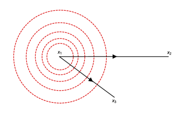
In the previous section, we computed the OPE coefficients for the two protected and one unprotected zero-magnon operator, see (4.16). In this section we generalize these results to the OPE coefficients of one protected and two unprotected zero-magnon operators .
We show below that these OPE coefficients can be easily obtained by gluing together the three-point correlation functions defined by , schematically 202020The factor on the r.h.s. comes from symmetrization in and .
| (8.1) |
where is an auxiliary light-like vector and
| (8.2) |
with dots denoting terms with derivatives acting on both fields. As usual, the normalization factor is fixed by the two-point function, . The stucture constant is given by (4.15) and (4.16) and the scaling dimension is defined in (4.1.2).
The three-point function (8.1) resums the wheel diagrams shown in Fig.17. They contain two scalar lines connecting with the two external points and dressed by an abritrary number of wheels incircling . We can use this result as a building block for a more complicated three-point correlation function, involving two twist-2 operators with an arbitrary spin and one protected operator
| (8.3) |
where is given by (8.2) with replaced with and (with ) being light-like vectors. In the planar limit, this correlation function receives contribution from the diagrams shown on Fig. 18. The main observation is that they can obtained by merging together two wheels depicted in Fig. 17.
To exemplify the idea we first consider (8.3) for . In this case, we have
| (8.4) |
where the operator amputates an extra propagator and the integration over glues two sets of wheels together. Here are the scaling dimensions of the operators and given by (4.10) but it is convenient to keep and to be arbitrary. 212121Note that we can in principle take different couplings of wheels around and around (similarly to Cavaglia:2018lxi ), i.e. and , making also and unequal. Then, after differentiation in the integral becomes
| (8.5) |
We can employ inversions to verify that the integral transforms under the conformal transformation as a three-point correlation function of scalar operators. This property fixes the form of up to a structure constant
| (8.6) |
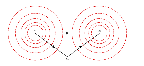
The integral in (8.5) can be computed immediately using the star-triangle identity leading to
| (8.7) |
Replacing with (4.16) we obtain the following expression
| (8.8) |
which is symmetric in and as it should be.
So far, we treated and as arbitrary parameters. We expect that, in the limit , when the correlator looses all its wheels around , it should reduce to the wheel correlation function (8.1) multiplied by a free scalar propagator connecting and . Indeed, it is easy to see that .
In application to the conformal fishnet theory, we have to replace the scaling dimensions in (8.8) with their exact expression (4.10). In this case, the expression (8.8) simplifies to
| (8.9) |
Non-zero spins.
It is straightforward to generalize (8.4) to the operators with non-zero spins
| (8.10) |
where the notation was introduced for the so-called conformal triangle function
| (8.11) |
In order to perform the integration in (8.10), we make use of the following identity
| (8.12) |
where is a differential operator acting on 222222A similar operator also appeared in Karateev:2017jgd .
| (8.13) |
and the normalization constant is given by
| (8.14) |
Replacing the functions in (8.10) with (8.12), we can pull out the differential operator outside the integral to obtain
| (8.16) | |||||
where the integral can be again computed using the star-triangle identity.
In this way, we arrive at the following expression
| (8.17) |
where the dependence on is carried by the function
| (8.18) |
The structure constant depends on the scaling dimensions and spins of the two unprotected operators and reads
| (8.19) | |||||
This relation constitutes the main result of this section. We can check again that in the limit and the general expression (8.19) reduces to defined in (4.15). We note that there is a striking similarity of (8.19) with the expressions for the cusp structure constants of Cavaglia:2018lxi ; Kim:2017sju .
The function describes the dependence of the three-point correlation function (8.3). Based on the conformal symmetry, we expect that it should have the following general form Costa:2011mg
| (8.20) |
where
| (8.21) |
and the sum runs over the conformal tensors projected onto light-like vectors and
| (8.22) |
The expansion coefficients can be found by matching (8.20) into (8.18)
| (8.23) |
Applying (8.19) we have to replace the scaling dimensions and by their explicit expressions. For the twist-two operators (8.2) they are given by the function , Eq. (4.1.2), evaluated for spin and , respectively. We recall that the scaling dimensions of twist-2 and twist-4 operators, and are two branches of the same function of the (complexified) coupling constant . This suggests that depending on the choice of the branch of the functions and , the relation (8.17) should also describe the three-point correlation function of the protected operator with two unprotected operators each having twist or twist.
9 Generalization to any dimension
Many of the results obtained in the previous sections for the bi-scalar theory (1.1) in dimensions can be easily generalized to its dimensional version proposed in Kazakov:2018qbr . In particular, the zero-magnon four-point correlation function was computed there for any , generalizing the results of Grabner:2017pgm .
The Lagrangian of dimensional bi-scalar model is non-local
| (9.1) |
where the differential operator in an arbitrary power is defined in a standard way, as an integral operator. For the particular “isotropic” case , the action (9.1) should be supplemented with the same double-trace counterterms (1.1). As before, the theory has two fixed points with the corresponding values of the double-trace couplings depending on and computable at least at weak coupling. Since the -dimensional theory (9.1) has the same chiral interaction vertex as (1.1), we can consider the correlation functions the same types as those shown on Fig.1. An important difference with the case is that free scalar propagators are now given by with .
To compute zero- and one-magnon four-point correlation functions, as it is done in 4 dimensions in the previous sections, we have to find, at any , the eigenvalues of the graph-building operators and . They are computed in appendix C leading to (see also Giombi:2017dtl ; Kazakov:2018qbr )
| (9.2) | |||
| (9.3) |
In addition, we also need the expression for the kinematical factor defined in (A.6). It is given in by (A.6), where we should take for the zero-magnon case and for the one-magnon case. Assuming that all the intermediate steps are still valid for general , we find the the following expression for the OPE coefficients
| (9.4) |
where , and , for zero-magnon and one-magnon cases, respectively. The dimension of operator appearing at the corresponding pole is related to the representation label in the following way: . For , the zero-magnon spectrum looks particularly simple Kazakov:2018qbr
| (9.5) |
Interestingly Kazakov:2018qbr , the particular case of with in (9.1) is relevant for the BFKL approximation in high-energy QCD.
For general the structure of the poles in could change. In particular the poles coming from will have a different number of solutions for different (actually, this number is infinite for odd dimensions, see Kazakov:2018qbr for the analysis of possible exchange states in zero-magnon case), and those have to be taken into account when computing the correlation function. The computations are particularly simple in dimensions , where is integer. Then the spectral equations become polynomial in . For example, for one-magnon case, the spectral equation for looks as
| (9.6) |
etc.
We leave the computations of a more complicated two-magnon correlation function, as well as the detailed study of the general case, for future investigation.
10 Discussion and Conclusions
In this work, we computed exactly and explicitly certain 4-point correlation functions in bi-scalar CFT (1.1) which represent a specific double scaling limit (combining weak coupling and strong imaginary twist) of -deformed SYM theory in ’t Hooft approximation Gurdogan:2015csr . Although this theory obeys the integrability properties, related to the integrability of fishnet Feynman graphs Zamolodchikov:1980mb dominating in its planar perturbation theory, we concentrate here on the physical quantities which can be computed without any appeal to the integrability and utilizing only the conformal symmetry properties. The three types of such 4-point functions are named as zero-magnon, one-magnon and two-magnon cases, referring to the exchange operators which are of a type , and , as well as their non-zero spin cousins. The last operator is the analogue of the famous Konishi operator in It is quite remarkable that we managed to compute explicitly the all-loop anomalous dimensions of all these operators, as well as their structure constants with the external protected operators. These formulas give a host of very non-trivial non-perturbative OPE data, with a rich analytic structure. To our knowledge, this are the first examples of such non-perturbatively and explicitly computed 4-point correlation functions in an interacting CFT in dimensions.
The results for 4-point functions are presented in a standard form, as explicit OPE expansions over conformal blocks. We studied these functions by the weak coupling expansion and found that the results for zero- and one-magnon cases can be presented, in each order of weak-coupling expansion, in terms of special class of functions called Harmonic Poly Logariphms (HPL), thus facilitating the study of these functions in the cross channels. As for the more complicated two-magnon case, we observed that the HPL representation is only possible in the light-cone limit , or equivalently with fixed.
Many interesting questions related to the study of these quantities are left out of the scope of this paper. In particular, we left for the future the study of the operator content and the OPE in cross-channels of all three 4-point functions, where the analytic structure looks more complicated than in the original channel. It would be also interesting to generalize these 4-point functions to the case of external operators with spins. The correlation functions we computed could serve as a building block for more complicated point functions by gluining them together. Similar approach was recently developed in SYK context in Gross:2017aos 232323see also Rosenhaus:2018dtp for a recent review.. To demonstrate the procedure we show in section 8 how to obtain more complicated structure constants starting from the elementary blocks.
Notice that the main common feature of the 4-point functions, which allowed for the explicit computations using the combination of Bethe-Salpeter techniques and the conformal symmetry, was the presence of not more than two scalar fields of each species, or , in the exchange operators. If we want to compute the multi-point correlation functions with more than two scalars of any of the species in exchange operators, we have to appeal to the integrability methods, based on the non-compact conformal Heisenberg type spin chains. All computations become then much more sophisticated, though in many cases possible. Already the computations of anomalous dimensions of operator and its cousins with the same -charge, necessitated the extraction of the results from the quantum spectral curve of the full -deformed SYM theory, in the corresponding double scaling limit Gromov:2017cja . The alternative method for computations of anomalous dimensions, is based on the integrable quantum conformal spin chain WithDavidToAppear . For the 3-point and 4-point correlation functions in bi-scalar theory, this last method seems to be particularly promising. Recently, in a very similar setup it was shown that the separation of variables (SOV) approach could be used to get compact expessions for the correlation function in Cavaglia:2018lxi . The expressions for the structure constants obtained there are very similar to our results, which indicates that a similar SOV-based approach could work here. There are also some other options, such as the form factor approach Basso:2015zoa , successfully applied in Basso:2017jwq for the computation of certain 4-point correlation function based on fishnet graphs with disc topology.
Interestingly, all our current results for 4-point correlation functions in dimensions appear to be directly generalizable to the bi-scalar CFT at any which was recently formulated in Kazakov:2018qbr . The case is closely related to the BFKL model of reggeized gluons describable by the Heisenberg spin chain Lipa:1993pmr ; Faddeev:1994zg ; Derkachov:2001yn ; DeVega:2001pu . It is worth noticing that the computations of 4- and 6-point correlation functions of BFKL pomeron light-ray operators presented in Balitsky:2013npa ; Balitsky:2015oux ; Balitsky:2015tca look closely related to our current computations. It would be interesting to compare those results to our current results.
The most interesting, physical questions about the bi-scalar CFT still remain to be answered. It still remains to be understood whether this theory has a dual string description. The availability of explicit all-loop results, such as presented in this paper, should allow for some guesses in this direction. Quite intriguingly, the strong coupling limit of the point correlators studied in this paper exhibits typical classical exponential scaling with the coupling, suggesting existence of the dual strong coupling classical description.
Note added:
while this paper was in preparation a paper Liu:2018jhs appeared about SYK model, which may however have some overlap with our results.
Acknowledgements
We are thankful to F. Aprile, B. Basso, J. Caetano, A. Cavaglia, S. Derkachev, J. Drummond, D. Grabner, O. Gurdogan, P. Heslop, D. Kosower, F. Levkovich-Maslyuk, E. Olivucci, M. Preti, V. Rosenhaus, E. Sobko for discussions. The work of V.K. was supported by the European Research Council (Programme “Ideas” ERC-2012-AdG 320769 AdS-CFT-solvable). N.G. and V.K. are grateful to Humboldt University (Berlin) for the hospitality and financial support of this work in the framework of the “Kosmos” programme. N.G. wishes to thank STFC for support from Consolidated grant number ST/J002798/1. The work of G.K. was supported by the French National Agency for Research grant ANR-17- CE31-0001-01. G.K. would like to thank the Galileo Galilei Institute for Theoretical Physics for the hospitality, the INFN and Simons Foundation for partial support during the completion of this work.
Appendix A Definitions and relations
In the main text we use the following definition of the four-dimensional conformal block Dolan:2000ut
| (A.1) | ||||
| (A.2) |
We also use the following formulas for normalization of the conformal triangles in any dimension
| (A.3) | ||||
where . The coefficients and enter into the general relations we discuss in the text. They are given by Tod:1977harm
| (A.4) | ||||
| (A.6) |
The functions form an orthogonal basis for . This implies the following resolution of identity
| (A.7) |
when projected to the functional space spanned by .
Appendix B Cancellation of the spurious poles
In this appendix we analyse additional possible contributions in (3.17) due to the extra poles in and the measure factor . We will see that these contributions cancel each other if an additional condition is imposed on the eigenvalue .
The conformal block from (A.1) has simple poles at (with ), or equivalently . Its residue at the pole is given by where (see for example Appendix B in Simmons-Duffin:2017nub ):
| (B.1) |
This results in the following extra contribution to (3.17):
| (B.2) |
The sum of the above contributions in general is not zero, however, there are also poles at coming from factor in (3.12). They can be also expressed in terms of as follows
| (B.3) |
resulting in another contribution
| (B.4) |
Let us show that these poles cancel under certain condition on . The sum of the contributions of can be written as
| (B.5) |
where we use that and in the last sum we shift the summation index by and renamed to . Since the other contribution has the form
| (B.6) |
we have to consider
| (B.7) |
We see that there will be no additional terms in (3.16) if we require
| (B.8) |
We verify in the main text that this requirement is indeed satisfied for each case considered.
Appendix C Eigenvalues of the graphs-building operators
In this appendix we give technical details of the derivation of the eigenvalues of the graphs-building operators , and .
C.1 Star-triangle identity
The calculation can be simplified by applying the so-called star-triangle identity
| (C.1) |
where the exponents , and satisfy . A particular case of it is
| (C.2) |
which can be obtained from (C.1) by sendind point to infinity.
C.2 Eigenvalue
Here we compute the eigenvalue of the graph-building operator corresponding to the correlation function in the -dimensional version of the bi-scalar theory.
In virtue of conformal symmetry, the eigenstate of is given by (3) with being scaling dimension of scalars in dimensions
The calculation of the eigenvalue of reduces to the following integral
| (C.3) |
where we used (4.2), generalised to any .
Firstly, we observe that the integrand simplifies by the change of variables (with )
| (C.4) |
corresponding to the inversion around . This results in the following integral
| (C.5) |
where in the second relation we replaced the factor of by derivatives acting on .
Next integrating by parts we can swap into the derivative in and pull it out of the integral
| (C.6) |
After that the integration can be performed by applying the star-triangle identity (C.2) twice, leading to
| (C.7) |
Evaluating the derivatives and comparing with (C.3) we arrive at
| (C.8) |
In the particular case we obtain (4.5). The last relation agrees with the results of Kazakov:2018qbr and generalizes the result of Grabner:2017pgm
C.3 Eigenvalue
The calculation of the eigenvalue of the graph-building operator for the correlation function is similar to the previous case. As before, we perform the calculation for general . The graph-building operator looks as
| (C.9) |
Its eigenstate is given by (3) with and
| (C.10) |
Like in the previous case, to find the eigenvalue we need to evaluate the integral
| (C.11) |
Again the integrand simplifies after the inversion around
| (C.12) |
Again we can absorb the last term under the integral into the derivatives in and evaluate the integral using (C.2)
| (C.13) |
Finally, computing the derivatives and comparing the result with (C.11) we arrive at
| (C.14) |
which reduces at to (4.29).
C.4 Eigenvalue
Introducing for convenience and defining dual coordinates, , and , we can rewrite (4.46) as a two-loop Feynman integral
| (C.15) |
where and . Due to symmetry of the integrand under , vanishes for odd .
For the integral (4.46) is known as a massless two-loop self-energy Feynman integral. It can be expressed in a closed form in terms of hypergeometric function (see e.g. review Grozin:2012xi )
| (C.16) |
This representation is not convenient however to elucidate analytic properties of , that why we derive below another equivalent representation.
We start with rewriting (C.15) with all Lorentz indices uncontracted
| (C.17) |
where denotes a symmetric traceless tensor and is even. Then, we project all Lorentz indices on the vector and take into account the identity
| (C.18) |
The coefficients can be found from the requirement for the expression on the right-hand side to vanish upon hitting it with . Replacing with in (C.18) we get
| (C.19) |
In this way, we obtain another representation for that differs from (C.15) in that is replaced by the expression on the right-hand side of (C.18) divided by the normalization factor that enters (C.19). The advantage of this representation is that we can use the identity
| (C.20) |
to express in terms of scalar Feynman integrals. Some of the integrals coincide with those contributing to whereas the remaining integrals have one propagator less and can be easily evaluated. As a consequence, is given by a linear combination of and some rational functions of .
Going through the calculation of for and we find
| (C.21) |
In general, for , we have
| (C.22) |
The solution to this recurrence relation looks as
| (C.23) |
Assuming that vanishes at large faster then (this property can be verified a posteriori) we find from (C.23) that is given by
| (C.24) | ||||
| (C.25) | ||||
We verified that the two representations (C.16) and (C.24) are equivalent.
Appendix D Analytic properties of the correlation functions
We can apply (3.11) and(3.12) to understand analytic properties of as a function of the coupling constant . The integrand of (3.12) is a meromorphic function of which is just a power of dependent on the type of the correlation function.
The integral in (3.12) is well-defined as soon as the physical poles (3.14) are away from the real axis. As soon as the physical pole (3.14) approaches the real axis, the integral (3.12) generates a branch cut in . The discontinuity across the cut can be found from (3.12)
| (D.1) |
In virtue of (3.13), the integral localizes at two points and satisfying (3.14). Taking into account (3.17) we obtain
| (D.2) |
According to (4.5) and (4.3.1), and are positive definite functions of and, therefore, the integral on the right-hand side of (D.1) vanishes for for zero- and two-magnon functions, and , respectively. Moreover, the function satisfies the relation on the real axis and, as a consequence, for .
Appendix E Renormalization group flow of the coupling constants
The -deformed SYM remains a unitary theory as long as the -deformation angles are real and all the couplings, ’t’Hooft coupling and the double-trace couplings, are real. On the other hand, this is not a CFT anymore since the real double-scaling couplings run with the scale even in the leading ’t Hooft limit. Looking at the leading order beta-function for the interaction term the one-loop beta-function is given by Fokken:2014soa
| (E.1) |
where and are the parameters of -twist, we expect the critical double-trace couplings at , where the theory is conformal, to have two complex conjugate fixed points
| (E.2) |
Using Callan-Symanzik RG equation we arrive, at the critical point, to the following complex anomalous dimension
| (E.3) |
At a finite , then two exact (in a given scheme) critical couplings are comnplex conjugate functions of :
| (E.4) |
where and are real functions of the couplping and .
It is interesting to understand how the vicinity of these critical points to the real axis may influence the RG flow of coupling (we remind that the ’t Hooft coupling stays fixed with RG, at least in the large limit). To get a better qualitative picture of what happens in -deformed SYM we can study the RG of the similar coupling in the bi-scalar model where we have more of the exact data, and only one coupling is running. The beta function for this coupling was computed in Grabner:2017pgm up to a few orders of PT in regularisation, in MS scheme, and the result is quadratic in , as was predicted in Pomoni:2008de for a generic large CFT of this type 242424 This mechanism was first established in Dymarsky:2005uh an the example of non-supersymmetric orbifold theories, with non-running single-trace four-scalar interaction and a running double trace coupling:
| (E.5) |
where and the functions , , and are given by
| (E.6) |
Moreover, there exists the following exact relation between the functions (E) and the scaling dimensions (4.32) at the fixed point Pomoni:2008de ; Grabner:2017pgm :252525This relation between the scaling dimension of the operator at the critical point and the discriminant of quadratic equation on zeros of the beta-function follows directly from the eqs.(2.47-48) of the paper Pomoni:2008de . It is valid for a generic large CFT of this type.
| (E.7) |
where is the anomalous dimension of at the corresponding fixed point, so that
| (E.8) |
where we introduced two real functions of
| (E.9) |
We can write the RG equation in the following form
| (E.10) |
Let us introduce a new coupling , as well as , which can be considered as changing the RG scheme. Then the RG equation can be written as
| (E.11) |
Solving this equation in this specially chosen renormalization scheme, we find an RG flow:
| (E.12) |
which is defined only through the universal quantity - the anomalous dimension . This type of RG flow for the double-trace coupling also first appeared in the papers Dymarsky:2005uh ; Pomoni:2008de .
The physical quantities of the theory have a cut along the half-axis and poles. For generic complex ’s there is no such problem. Assuming the coupling to have a little negative imaginary the RG flow (E.12) will avoid the poles in the r.h.s. and interpolate between two fixed point or (one of them is IR fixed point, another is the UV fixed point, depending on the sign of ). We illustrate the possible RG flows in Fig.19.
References
- (1) S. Rychkov, EPFL Lectures on Conformal Field Theory in D>= 3 Dimensions, SpringerBriefs in Physics. 2016, 10.1007/978-3-319-43626-5, [1601.05000].
- (2) M. Shaposhnikov and A. Shkerin, Conformal symmetry: towards the link between the Fermi and the Planck scales, 1803.08907.
- (3) V. M. Braun, G. P. Korchemsky and D. Mueller, The Uses of conformal symmetry in QCD, Prog. Part. Nucl. Phys. 51 (2003) 311 [hep-ph/0306057].
- (4) P. Di Francesco, P. Mathieu and D. Senechal, Conformal Field Theory, Graduate Texts in Contemporary Physics. Springer-Verlag, New York, 1997, 10.1007/978-1-4612-2256-9.
- (5) J. M. Maldacena, The Large N limit of superconformal field theories and supergravity, Int. J. Theor. Phys. 38 (1999) 1113 [hep-th/9711200].
- (6) R. G. Leigh and M. J. Strassler, Exactly marginal operators and duality in four-dimensional N=1 supersymmetric gauge theory, Nucl. Phys. B447 (1995) 95 [hep-th/9503121].
- (7) O. Lunin and J. M. Maldacena, Deforming field theories with U(1) x U(1) global symmetry and their gravity duals, JHEP 0505 (2005) 033 [hep-th/0502086].
- (8) V. Kazakov, S. Leurent and D. Volin, T-system on T-hook: Grassmannian Solution and Twisted Quantum Spectral Curve, 1510.02100.
- (9) C. Cordova, T. T. Dumitrescu and K. Intriligator, Multipletsltiplets of Superconformal Symmetry in Diverse Dimensions, arXiv:1612.00809 (2016) 165 [1506.03807].
- (10) C. Cordova, T. T. Dumitrescu and K. Intriligator, Multiplets of Superconformal Symmetry in Diverse Dimensions, arXiv:1612.00809 11 (2016) 135 [1602.01217].
- (11) C. Cordova, T. T. Dumitrescu and K. Intriligator, Deformations of Superconformal Theories, JHEP 11 (2016) 135 [1602.01217].
- (12) N. Beisert, B. Eden and M. Staudacher, Transcendentality and Crossing, J. Stat. Mech. 0701 (2007) P01021 [hep-th/0610251].
- (13) N. Gromov, V. Kazakov and P. Vieira, Exact Spectrum of Anomalous Dimensions of Planar N=4 Supersymmetric Yang-Mills Theory, Phys. Rev. Lett. 103 (2009) 131601 [0901.3753].
- (14) N. Beisert et al., Review of AdS/CFT Integrability: An Overview, Lett. Math. Phys. 99 (2012) 3 [1012.3982].
- (15) C. Andrea, D. Fioravanti, N. Gromov and R. Tateo, Quantum Spectral Curve of the 6 Supersymmetric Chern-Simons Theory, Phys. Rev. Lett. 113 (2014) 021601 [1403.1859].
- (16) N. Gromov, V. Kazakov, S. Leurent and D. Volin, Quantum Spectral Curve for Planar Super-Yang-Mills Theory, Phys. Rev. Lett. 112 (2014) 011602.
- (17) N. Gromov, V. Kazakov, S. Leurent and D. Volin, Quantum spectral curve for arbitrary state/operator in AdS5/CFT4, JHEP 09 (2015) 187 [1405.4857].
- (18) N. Gromov, Introduction to the Spectrum of SYM and the Quantum Spectral Curve, 1708.03648.
- (19) V. Kazakov, Quantum Spectral Curve of -twisted SYM theory and fishnet CFT, 1802.02160.
- (20) J. Escobedo, N. Gromov, A. Sever and P. Vieira, Tailoring Three-Point Functions and Integrability, JHEP 09 (2011) 028 [1012.2475].
- (21) B. Basso, S. Komatsu and P. Vieira, Structure Constants and Integrable Bootstrap in Planar N=4 SYM Theory, 1505.06745.
- (22) A. Cavaglia, N. Gromov and F. Levkovich-Maslyuk, Quantum Spectral Curve and Structure Constants in N=4 SYM: Cusps in the Ladder Limit, 1802.04237.
- (23) S. Giombi and S. Komatsu, Exact Correlators on the Wilson Loop in SYM: Localization, Defect CFT, and Integrability, 1802.05201.
- (24) T. Fleury and S. Komatsu, Hexagonalization of Correlation Functions, JHEP 01 (2017) 130 [1611.05577].
- (25) B. Eden and A. Sfondrini, Tessellating cushions: four-point functions in = 4 SYM, JHEP 10 (2017) 098 [1611.05436].
- (26) D. Correa, J. Maldacena and A. Sever, The quark anti-quark potential and the cusp anomalous dimension from a TBA equation, JHEP 08 (2012) 134 [1203.1913].
- (27) N. Gromov and F. Levkovich-Maslyuk, Quantum Spectral Curve for a Cusped Wilson Line in N=4 SYM, 1510.02098.
- (28) T. Bargheer, J. Caetano, T. Fleury, S. Komatsu and P. Vieira, Handling Handles I: Nonplanar Integrability, 1711.05326.
- (29) T. Banks and A. Zaks, On the Phase Structure of Vector-Like Gauge Theories with Massless Fermions, Nucl. Phys. B196 (1982) 189.
- (30) S. El-Showk, M. F. Paulos, D. Poland, S. Rychkov, D. Simmons-Duffin and A. Vichi, Solving the 3D Ising Model with the Conformal Bootstrap, Phys. Rev. D86 (2012) 025022 [1203.6064].
- (31) R. Rattazzi, V. S. Rychkov, E. Tonni and A. Vichi, Bounding scalar operator dimensions in 4D CFT, JHEP 12 (2008) 031 [0807.0004].
- (32) S. Frolov, Lax pair for strings in Lunin-Maldacena background, JHEP 05 (2005) 069 [hep-th/0503201].
- (33) N. Beisert and R. Roiban, Beauty and the twist: The Bethe ansatz for twisted N=4 SYM, JHEP 08 (2005) 039 [hep-th/0505187].
- (34) C. Sieg and M. Wilhelm, On a CFT limit of planar -deformed SYM theory, Phys. Lett. B756 (2016) 118 [1602.05817].
- (35) D. Grabner, N. Gromov, V. Kazakov and G. Korchemsky, Strongly gamma-deformed N=4 SYM as an integrable CFT, 1711.04786.
- (36) A. A. Tseytlin and K. Zarembo, Effective potential in nonsupersymmetric SU(N) x SU(N) gauge theory and interactions of type 0 D3-branes, Phys. Lett. B457 (1999) 77 [hep-th/9902095].
- (37) Q. Jin, The Emergence of Supersymmetry in -deformed super-Yang-Mills theory, 1311.7391.
- (38) J. Fokken, C. Sieg and M. Wilhelm, Non-conformality of -deformed N = 4 SYM theory, J. Phys. A47 (2014) 455401 [1308.4420].
- (39) J. Fokken, C. Sieg and M. Wilhelm, A piece of cake: the ground-state energies in -deformed = 4 SYM theory at leading wrapping order, JHEP 09 (2014) 78 [1405.6712].
- (40) N. Gromov and F. Levkovich-Maslyuk, Y-system and -deformed N=4 Super-Yang-Mills, J. Phys. A44 (2011) 015402 [1006.5438].
- (41) C. Ahn, Z. Bajnok, D. Bombardelli and R. I. Nepomechie, TBA, NLO Luscher correction, and double wrapping in twisted AdS/CFT, JHEP 12 (2011) 059 [1108.4914].
- (42) O. Gurdogan and V. Kazakov, New integrable non-gauge 4D QFTs from strongly deformed planar N=4 SYM, 1512.06704.
- (43) J. Caetano, O. Gurdogan and V. Kazakov, Chiral limit of N = 4 SYM and ABJM and integrable Feynman graphs, 1612.05895.
- (44) N. Gromov, V. Kazakov, G. Korchemsky, S. Negro and G. Sizov, Integrability of conformal fishnet theory, arXiv:1706.04167 [hep-th] .
- (45) D. Chicherin, V. Kazakov, F. Loebbert, D. Mueller and D.-l. Zhong, Yangian Symmetry for Bi-Scalar Loop Amplitudes, 1704.01967.
- (46) D. Chicherin, V. Kazakov, F. Loebbert, D. Mueller and D.-l. Zhong, Yangian Symmetry for Fishnet Feynman Graphs, Phys. Rev. D96 (2017) 121901 [1708.00007].
- (47) V. Kazakov and E. Olivucci, Bi-scalar integrable CFT at any dimension, 1801.09844.
- (48) A. B. Zamolodchikov, ’FISHNET’ DIAGRAMS AS A COMPLETELY INTEGRABLE SYSTEM, Phys. Lett. 97B (1980) 63.
- (49) N. Gromov and F. Levkovich-Maslyuk, Quark-anti-quark potential in 4 SYM, JHEP 12 (2016) 122 [1601.05679].
- (50) S. E. Derkachov, G. P. Korchemsky and A. N. Manashov, Noncompact Heisenberg spin magnets from high-energy QCD: 1. Baxter Q operator and separation of variables, Nucl. Phys. B617 (2001) 375 [arXiv:0107193 [hep-th]].
- (51) H. J. De Vega and L. N. Lipatov, Interaction of reggeized gluons in the Baxter-Sklyanin representation, Phys. Rev. D64 (2001) 114019 [hep-ph/0107225].
- (52) B. Basso and L. J. Dixon, Gluing Ladder Feynman Diagrams into Fishnets, Phys. Rev. Lett. 119 (2017) 071601 [1705.03545].
- (53) V. K. Dobrev et al., Harmonic analysis on the n-dimensional lorentz group and its application to conformal quantum field theory, Lect.Notes Phys. 63 12 (1977) 059.
- (54) F. A. Dolan and H. Osborn, Conformal Partial Waves: Further Mathematical Results, Phys. Lett 718 (2011) 169 [arXiv:1108.6194 [hep-th]].
- (55) F. A. Dolan and H. Osborn, Conformal four point functions and the operator product expansion, Nucl. Phys. B599 (2001) 459 [arXiv:0011040 [hep-th]].
- (56) G. P. Korchemsky, On level crossing in conformal field theories, JHEP 03 (2016) 212 [1512.05362].
- (57) J. Escobedo, N. Gromov, A. Sever and P. Vieira, Tailoring three-point functions and integrability, 1012.2475v2.
- (58) N. Gromov and P. Vieira, Tailoring three-point functions and integrability iv. theta-morphism, 1205.5288v1.
- (59) J. Caetano, “To be published.”.
- (60) F. C. S. Brown, Polylogarithmes multiples uniformes en une variable, Compt. Rend. Math. 338 (2004) 527.
- (61) L. J. Dixon, C. Duhr and J. Pennington, Single-valued harmonic polylogarithms and the multi-Regge limit, JHEP 10 (2012) 074 [1207.0186].
- (62) E. Remiddi and J. A. M. Vermaseren, Harmonic polylogarithms, Int. J. Mod. Phys. A15 (2000) 725 [hep-ph/9905237].
- (63) D. Maitre, HPL, a mathematica implementation of the harmonic polylogarithms, Comput. Phys. Commun. 174 (2006) 222 [hep-ph/0507152].
- (64) N. Gromov, A. Sever and P. Vieira, Tailoring Three-Point Functions and Integrability III. Classical Tunneling, JHEP 07 (2012) 044 [1111.2349].
- (65) Y. Kazama and S. Komatsu, Wave functions and correlation functions for GKP strings from integrability, JHEP 09 (2012) 022 [1205.6060].
- (66) B. Basso and D.-l. Zhong, Continuum limit of fishnet graphs and AdS sigma model, 1806.04105.
- (67) M. Hogervorst and S. Rychkov, Radial Coordinates for Conformal Blocks, Phys. Rev. D87 (2013) 106004 [1303.1111].
- (68) D. Medina-Rincon, A. A. Tseytlin and K. Zarembo, Precision matching of circular Wilson loops and strings in AdS S5, JHEP 05 (2018) 199 [1804.08925].
- (69) V. A. Kazakov, A. Marshakov, J. A. Minahan and K. Zarembo, Classical/quantum integrability in ads/cft, hep-th/0402207v6.
- (70) N. Beisert, V. A. Kazakov, K. Sakai and K. Zarembo, The algebraic curve of classical superstrings on ads_5xs^5, hep-th/0502226v3.
- (71) V. A. Kazakov and K. Zarembo, Classical/quantum integrability in non-compact sector of ads/cft, hep-th/0410105v3.
- (72) D. Karateev, P. Kravchuk and D. Simmons-Duffin, Weight Shifting Operators and Conformal Blocks, JHEP 02 (2018) 081 [1706.07813].
- (73) M. Kim, N. Kiryu, S. Komatsu and T. Nishimura, Structure Constants of Defect Changing Operators on the 1/2 BPS Wilson Loop, JHEP 12 (2017) 055 [1710.07325].
- (74) M. S. Costa, J. Penedones, D. Poland and S. Rychkov, Spinning Conformal Correlators, JHEP 11 (2011) 071 [1107.3554].
- (75) S. Giombi, I. R. Klebanov and G. Tarnopolsky, Bosonic tensor models at large and small , Phys. Rev. D96 (2017) 106014 [1707.03866].
- (76) D. J. Gross and V. Rosenhaus, All point correlation functions in SYK, JHEP 12 (2017) 148 [1710.08113].
- (77) V. Rosenhaus, An introduction to the SYK model, 1807.03334.
- (78) D. Grabner, N. Gromov, V. Kazakov and G. Korchemsky, to appear, .
- (79) L. N. Lipatov, High energy asymptotics of multi-color QCD and exactly sol vable lattice models, JETP Lett. 59 (1994) 596-599; 12 (1994) 059 [arXiv:9311037v1 [hep-th]].
- (80) L. D. Faddeev and G. P. Korchemsky, High-energy QCD as a completely integrable model, Phys. Lett. B342 (1995) 311 [hep-th/9404173].
- (81) I. Balitsky, V. Kazakov and E. Sobko, Two-point correlator of twist-2 light-ray operators in N=4 SYM in BFKL approximation, 1310.3752.
- (82) I. Balitsky, V. Kazakov and E. Sobko, Three-point correlator of twist-2 light-ray operators in N=4 SYM in BFKL approximation, 1511.03625.
- (83) I. Balitsky, V. Kazakov and E. Sobko, Structure constant of twist-2 light-ray operators in the Regge limit, Phys. Rev. D93 (2016) 061701 [1506.02038].
- (84) J. Liu, E. Perlmutter, V. Rosenhaus and D. Simmons-Duffin, -dimensional SYK, AdS Loops, and Symbols, 1808.00612.
- (85) D. Simmons-Duffin, D. Stanford and E. Witten, A spacetime derivation of the Lorentzian OPE inversion formula, 1711.03816.
- (86) A. G. Grozin, Massless two-loop self-energy diagram: Historical review, Int. J. Mod. Phys. A27 (2012) 1230018 [1206.2572].
- (87) E. Pomoni and L. Rastelli, Large N Field Theory and AdS Tachyons, JHEP 04 (2009) 020 [0805.2261].
- (88) A. Dymarsky, I. R. Klebanov and R. Roiban, Perturbative search for fixed lines in large N gauge theories, JHEP 08 (2005) 011 [hep-th/0505099].