Optimal control theory for quantum electrodynamics: an initial state problem

Abstract

In conventional quantum optimal control theory, the parameters that determine an external field are optimised to maximise some predefined function of the trajectory, or of the final state, of a matter system. The situation changes in the case of quantum electrodynamics, where the degrees of freedom of the radiation field are now part of the system. In consequence, instead of optimising an external field, the optimal control question turns into a optimisation problem for the many-body initial state of the combined matter-photon system. In the present work, we develop such a optimal control theory for quantum electrodynamics. We derive the equation that provides the gradient of the target function, which is often the occupation of some given state or subspace, with respect to the control variables that define the initial state. We choose the well-known Dicke model to study the possibilities of this technique. In the weak coupling regime, we find that Dicke states are the optimal matter states to reach Fock number states of the cavity mode with large fidelity, and vice versa, that Fock number states of the photon modes are the optimal states to reach the Dicke states. This picture does not prevail in the strong coupling regime. We have also considered the extended case with more than one mode. In this case, we find that increasing the number of two-level systems allows to reach a larger occupation of entangled photon targets.

I Introduction

The coherent control of the dynamics of quantum systems Brumer and Shapiro (2003) is frequently theoretically approached within the framework of quantum optimal control theory Brif et al. (2010) (QOCT), the subset of optimal control theory Kirk (1998) applicable to quantum processes. It is concerned with the identification of parameters of the Hamiltonian of a system that induce a pre-defined optimal behaviour, such as the maximal occupation of an excited state, the dissociation of a molecule, etc. Often, those parameters – the control variables – determine the temporal shape of an external field present in the Hamiltonian – the control function. For example, the control problem may be the identification of some laser field shape (described classically) that prepares a quantum system in a desired state.

This formulation assumes that the controlling field is external, and its source is not affected by the system evolution. If, instead, one needs to describe the coupled evolution of a piece of matter (atom, molecule, etc.) and an electromagnetic field, the dynamical system must in fact be composed of both. This is the situation, for example, in the field of cavity quantum electrodynamics (CQED) Walther et al. (2006) or in quantum optics in general. An atom or molecule trapped in a cavity and the electromagnetic cavity radiation form, in principle, a closed system, and no external control can be exercised: once the initial state is set, the evolution is fixed. Of course, one may then introduce an additional and external classical field, or a temporal variation of the system couplings, that can be controlled in some way. In this way, the formulation of the control problem would still be the traditional one (see Refs. Rojan et al. (2014); Deffner (2014); Allen et al. (2017), for example).

However, one may be interested in finding the optimal cavity field that induces a given matter subsystem behaviour. In this case, the control formulation apparently changes, as the control variables should be set to define the initial state of the field: the task is to find the initial field state such that the coupled evolution is optimal with respect to the goal. And, once the field and the matter subsystem are treated on the same footing, one may pose an inverse control problem: find the optimal matter system state that induces the creation of a given photon field. In any case, the task has changed: from manipulating parameters that determine the Hamiltonian (or, in general, the dynamical function), to manipulating parameters that determine the initial state. Fortunately, it is known that the two problems are mathematically exactly equivalent. Using this formal equivalence, we will present working equations for the optimal-initial-state problem. Note that the two points of view are not exclusive, and one may use the formalism described below also for open systems subject to external fields – or subject to dissipation.

The objective of this work is to explore, numerically, the control technique in this apparently new formulation. For that purpose we have focused on a relevant quantum optical model: the Dicke Hamiltonian Dicke (1954); Garraway (2011), that describes a set of two-level-systems (TLS) coupled to a single cavity mode – or more than one mode, in extended versions of the model. Originally, it was introduced to explain superradiant emission. Although hard to realise experimentally, there is interest in it because of the possibility of creating very entangled matter and photon states, and because of its phase transitions.

For the present work, we have designed the following numerical experiments: (1) find the optimal initial photon field such that the evolution of the system, assuming the TLS set enters the cavity in its ground state, produces a Dicke or $W$ state Dicke (1954); Dür et al. (2000); and, inversely, (2) find the optimal TLS set initial state such that the evolution of the system, assuming a vacuum initial photon field, produces a photonic Fock state – or a combination of Fock states in a multi-mode setup.

Section II presents the basic theoretical discussion underlying the following calculations; Section III introduces the physical model, and the relevant states; Section IV describes the optimisation results, and finally conclusions are summarised in Section V.

II Optimal Control versus Initial State Preparation

We start by stating a simple formulation of the usual (quantum) optimal control problem Brif et al. (2010); Werschnik and Gross (2007); Peirce et al. (1988); Tersigni et al. (1990); Castro et al. (2012). Let $y$ be a Hilbert state vector that evolves according to the evolution law:

$$\dot{y}(t) = -{\rm i}\hat{H}(u,t)y(t)+b(u,t)\,,$$ (1)

$$y(0) = y^{0}\,.$$ (2)

The Hamiltonian $\hat{H}(u,t)$ depends on a set of parameters, the control variables $u_{1},\dots,u_{m}$. Note, that we have added an extra inhomogeneous term $b(u,t)$ that will become useful below, although it is obviously not present in a normal Schrödinger equation. More general quantum evolutions could be considered, e.g. open systems through the incorporation of stochastic terms, or via the use of Lindblad equations. Sometimes, instead of a discrete set of control variables $u_{1},\dots,u_{m}$ one considers one or more continuous control functions $u(t)$ as the objects of optimisation .

The system evolves until time $T$. One may then define a performance measure, or target functional $J$:

$$J(y,u)=F(y(T),u)+\int_{0}^{T}\!\!{\rm d}t\;G(y(t),u,t)\,,$$ (3)

whose maximisation is defined as the optimal system behaviour. In general it may contain the two terms shown in Eq. (3). The first term only depends on the final state of the system, whereas the second one depends on the full trajectory. In the following, we will only consider the presence of the first term $F$.

The specification of a control $u$ determines the system trajectory, $u\to y_{u}$. The optimal control problem may then be formulated as the identification of the maximum of the function

$$G(u)=F(y_{u}(T),u)\,.$$ (4)

Often, the control variables $u$ parametrize the shape of an external field; the problem is therefore finding the best external field that induces a given system reaction. However, if the field cannot be considered to be external, but must be included as a part of the full state description, the evolution is fixed once the initial state is specified. Finding the best external field means in this case shaping its initial state. The control problem must then be formulated for a system with the form:

$$\dot{z}(t) = -{\rm i}\hat{H}z(t)\,,$$ (5)

$$z(0) = z^{0}(u)\,,$$ (6)

or, more compactly, $z(t)=\hat{U}(t,0)z^{0}(u)$, where $\hat{U}(t_{1},t_{2})=$ $\exp(-{\rm i}(t_{1}-t_{2})\hat{H})$ is the evolution operator. The control variables $u$ now parametrize an initial state, and not the Hamiltonian $\hat{H}$. But they also determine the evolution of the system, $u\to z_{u}$, so that one may pose the problem of the optimisation of a functional $\tilde{F}(z_{u}(T),u)$. Although it is an apparently different formulation of the problem to the previous one, it can however be transformed into it via the change of variable:

$$y(t)=z(t)-z^{0}(u)\,,$$ (7)

that transforms Eqs. (5-6) into:

$$\dot{y}(t) = -{\rm i}\hat{H}y(t)-{\rm i}\hat{H}z^{0}(u)\,,$$ (8)

$$y(0) = 0\,,$$ (9)

i.e. they have the structure of Eqs. (1-2). One may then employ the usual machinery of QOCT in order to arrive, for example, at an equation for the gradient of the function $G(u)=\tilde{F}(z_{u}(T),u)$:

$$\frac{\partial G}{\partial u_{k}} = 2{\rm Re}\langle\frac{\partial\tilde{F}}{\partial z^{*}}(z_{u}(T),u)|\hat{U}(T,0)|\frac{\partial z^{0}}{\partial u_{k}}\rangle$$ (10)

$$+\left.\frac{\partial\tilde{F}}{\partial u_{k}}(z(T),u)\right|_{z(T)=z_{u}(T)}\,.$$

Details of the derivation of this equation are given in the appendix.

The previous result is rather general. It may be simplified if we assume that (i) the target functional takes the form:

$$\tilde{F}(z(T),u)=\langle z(T)|\hat{O}|z(T)\rangle\,,$$ (11)

where $\hat{O}$ is some observable (e.g. projection onto some subspace), and (ii) the variables $u$ are the (complex) expansion coefficients of the initial state in terms of the orthonormal basis of some subspace:

$$z^{0}(u)=\sum_{i}u_{i}\psi_{i}\,.$$ (12)

The function to optimise is then:

$$G(u)=\langle z^{0}(u)|\hat{U}(0,T)\hat{O}\hat{U}(T,0)|z^{0}(u)\rangle\,,$$ (13)

and due to both the linearity of $\hat{U}$ and the linearity of the previous definition of $z^{0}(u)$ with respect to $u$, the function $G$ may then be written as a quadratic form:

$$G(u)=\sum_{ij}u^{*}_{i}u_{j}\lambda_{ij}=u^{\dagger}{\bf\lambda}u\,,$$ (14)

where

$$\lambda_{ij}=\langle\psi_{i}|\hat{U}(0,T)\hat{O}\hat{U}(T,0)|\psi_{j}\rangle\,.$$ (15)

The search for an optimal $u$ cannot be unconstrained, since we must assume that the initial state is normalised, i.e. $u^{\dagger}u=1$. A quadratic form constrained in such a way has its critical points at its eigenvectors:

$$\lambda u=\mu u\,.$$ (16)

One may then choose the largest eigenvalue $\mu_{0}$ and its corresponding eigenvector $u_{0}$, as the solution of the maximisation problem:

$$G_{0}=G(u_{0})=\max_{u^{\dagger}u=1}\langle z_{u}(T)|\hat{O}|z_{u}(T)\rangle\,.$$ (17)

Numerically, the cost of the algorithm amounts to the cost of propagating each basis element $\psi_{j}$ separately in order to compute the matrix elements [Eq. 15], plus the cost of the matrix diagonalisation. This is the procedure that we will use in the examples below.

III Model

The Dicke Hamiltonian Dicke (1954); Garraway (2011) models $N$ atoms (in fact, generically speaking, TLSs of whatever origin) interacting with a single mode of the radiation field (the extension to more than one mode will discussed later on). It can be considered as a generalisation of the Rabi model, for which $N=1$. It is given by:

$$\hat{H}=\omega\hat{a}^{\dagger}\hat{a}+\omega_{0}\hat{J}_{z}+g(\hat{a}^{\dagger}+\hat{a})(\hat{J}_{+}+\hat{J}_{-})\,.$$ (18)

It describes a single cavity mode (whose frequency is $\omega$, and whose creation and annihilation operators are $\hat{a}^{\dagger}$ and $\hat{a}$, respectively), coupled to a set of $N$ TLSs. The $\hat{J}_{z}$ and $\hat{J}_{\pm}$ operators are the collective operators describing those:

$$\hat{J}_{z}=\frac{1}{2}\sum_{i}^{N}\hat{\sigma}_{z}^{(i)}$$ (19)

is the “population operator”, that sums all the Pauli $\sigma_{z}$ operators acting on each TLS $i$ (whose energy is $\omega_{0}$, although in the following we will always assume the resonance condition, $\omega_{0}=\omega$), and

$$\hat{J}_{\pm}=\frac{1}{2}\sum_{i}^{N}\hat{\sigma}_{\pm}^{(i)}$$ (20)

are the collective “ladder” operators. The basis states for each TLS are $|\downarrow\rangle$ and $|\uparrow\rangle$. The constant $g$ is the atom-cavity coupling constant. Assuming that the system is truly closed (all possible decay rates are negligible), the ratio $g/\omega$ determines whether (i) the model operates in the regime of validity of the rotating wave approximation (RWA), that permits to ignore the counter-rotating terms ($\hat{a}\hat{J}_{-}$ and $\hat{a}^{\dagger}\hat{J}_{+}$), i.e.:

$$\hat{H}\approx\hat{H}_{\rm TC}=\omega\hat{a}^{\dagger}\hat{a}+\omega_{0}\hat{J}_{z}+\frac{1}{2}g(\hat{a}^{\dagger}\hat{J}_{-}+\hat{a}\hat{J}_{+})\,,$$ (21)

or (ii) the model operates in the ultrastrong regime and the full Hamiltonian has to be considered. In Eq. (21), “TC” stands for Tavis and Cummings Tavis and Cummings (1968, 1969). For $N=1$, the TC model reduces to the analytically solvable Jaynes-Cummings model Jaynes and Cummings (1963); Shore and Knight (1993).

The coupling constant $g$ has another physical meaning: it is the Rabi frequency for this latter Jaynes-Cummings model: a system departing from the $|\downarrow\rangle\otimes|n\rangle$ state oscillates, with frequency $n^{1/2}g$, between this and the $|\uparrow\rangle\otimes|n-1\rangle$ state (where $|n\rangle$ and $|n-1\rangle$ are the photon Fock states with $n$ and $n-1$ photons, respectively).

Various physical systems have been found to be good candidates to realise the Dicke model. For example, the experiments on Rydberg-excited atoms passing through cavities Raimond et al. (2001); although many of these experiments have focused on the single atom and on the micromaser Meschede et al. (1985) concept, collective multi-atom effects have also been observed Raimond et al. (1982). A different frequency regime is that of optical cavities, which may also be well described by the Dicke Hamiltonian in appropriate circumstances Agarwal (1998). Both the Rydberg atom and the optical cavity setup, however, typically have a flux of atoms, and not a constant number as one tends to assume theoretically. This inconvenience is absent in the ion traps Härkönen et al. (2009) experiments – although the decay rates can be high. Finally, we mention circuit QED, that places superconducting qubits (instead of atoms) inside waveguides at microwave frequencies; the Dicke model can also be used for these systems Fink et al. (2009).

In the next section, we will show how the preparation of some initial states may lead to the creation of other target states – that could in turn be used as initial states for subsequent processes. For that purpose, we have focused on two sets of target states:

• Fock states, also known as number states, are perhaps the most “quantum” states of light (and of harmonic oscillators in general), as they are the states with a definite number of light quanta, i.e. photons. These states have potential applications in quantum metrology, cryptography and computing. Unfortunately, the creation of Fock states is challenging, and numerous protocols have been proposed, e.g. Refs. França Santos et al. (2001); Bertet et al. (2002); Brown et al. (2003); Zhang et al. (2012), or Ref. Hofheinz et al. (2008) for Fock states in a superconducting quantum circuit.

• Given a number $N$ of TLSs, the Dicke states Dicke (1954) are defined as:

  $$|D(N,k)\rangle={N\choose k}^{-\frac{1}{2}}{\rm sym}\left[|\downarrow\rangle^{\otimes N-k}\otimes|\uparrow\rangle^{\otimes k}\right]\,,$$ (22)

  where ${\rm sym}$ means symmetrisation. A Dicke state is therefore the equal superposition of all basis states of $N$ qubits having exactly $k$ excitations ($|\uparrow\rangle$ states). For the case $k=1$ (only one excitation), the Dicke states are also called $W$-states Dür et al. (2000): $W(N)=D(N,1)$. For example, assuming a TLS set with three systems ($N=3$):

  $$|W(3)\rangle=3^{-1/2}\left[|\uparrow\rangle\otimes|\downarrow\rangle\otimes|\downarrow\rangle+|\downarrow\rangle\otimes|\uparrow\rangle\otimes|\downarrow\rangle+|\downarrow\rangle\otimes|\downarrow\rangle\otimes|\uparrow\rangle\right]\,.$$ (23)

  Dicke states play an important role in quantum optics and quantum information theories, due to their entanglement and nonlocality Barnea et al. (2015). They have been prepared experimentally in various ways – see for example Ref. Wu et al. (2017) and references therein.

IV Results

IV.1 Creation of one-photon Fock states

We start with a simple example: the goal is to create the one photon Fock number state in an empty cavity, by tailoring the initial TLS set state that enters at time zero. Therefore, the initial parametrization of the initial state is given by:

$$|z^{0}(u)\rangle=\sum_{i}u_{i}|\phi_{i}\rangle\otimes|0\rangle$$ (24)

where $i$ runs over all the possible TLS set basis states $|\phi_{i}\rangle$, and $|0\rangle$ is the photon vacuum. The operator $\hat{O}$ that determines the target is in this case given by:

$$\hat{O}=\hat{I}_{\rm M}\otimes|1\rangle\langle 1|\,.$$ (25)

where $\hat{I}_{\rm M}$ is the identity operator in the “matter” space (the set of TLSs).

We have first set the coupling constant $g$ to a small value, well within the RWA validity range (weak coupling regime): $g/\omega=10^{-6}$, consistent for example with the experimental setups described in Ref. Raimond et al. (2001). For $N=1$ TLS, we would therefore have the Jaynes-Cummings Hamiltonian, whose evolution is analytically known, and the optimisation problem could be solved without any calculation: if the TLS enters the system in its excited state $|\uparrow\rangle$, the full system oscillates from $|\uparrow\rangle\otimes|0\rangle$ to $|\downarrow\rangle\otimes|1\rangle$ and back with frequency $g$ and period $\tau=\frac{2\pi}{g}$. If the total time is then set to half that period, the target state achieves full population for the $|\uparrow\rangle\otimes|0\rangle$ initial state.

This full population can only be achieved by fixing $T$ to that transition time, or odd multiples of it. At any other time, the optimal population would be lower, as it strongly depends on $T$. This fact also holds for larger $N$ values: for example, in Fig. 1 (top) we display the optimal population of the one-photon Fock state obtained when performing optimisations at varying values of $T$, for the $N=5$ case. The blue data in Fig. 1 corresponds to the results in the weak coupling regime. One may see how the full population can only be achieved at certain values of $T$. This fact suggest adding $T$ to the set of control variables, as it is a parameter that can often be controlled in experimental realisations of these models. This could be formally done generalising the previous equations from the beginning, but in our case we have preferred to do two consecutive searches: first, optimisations at fixed $T$ values as described above in order to build a $G_{0}(T)$ curve, and then one search for the maxima of this curve (named $T_{0}^{j}$ in the plot, where the index $j$ orders the local maxima in time).

For example, one could be interested in finding the fastest way to create the one-photon state. This would be achieved by using the optimal initial state that produces the first local maximum of the curve shown in Fig. 1, i.e. $T_{0}^{1}$. The evolution of $\langle\hat{O}\rangle(t)$ for the various optimal initial states are depicted in Fig. 1 (bottom, blue lines for the results obtained within the weak coupling regime).

By repeating this process with varying values of number of TLSs $N$, we found that: (i) in all cases, the one-photon Fock state could be produced exactly; (ii) the optimal initial state corresponding to the fastest transition is given by the $W(N)$ state; and (iii) the optimal interaction time follows a simple rule $T_{0}^{1}(N)=\frac{1}{2}N^{-1/2}\tau$. The time required for the one-photon state to be created is smaller as the number of TLSs grows.

We next explored in the same way the ultrastrong regime, by doing the same optimisation runs with values of $g\approx 0.5\omega$. The results are displayed in red in Fig. 1. The findings above do not hold: (i) in the ultrastrong regime, the perfect creation of the one photon state is not achieved (the best local maxima is $\approx$ 0.94), (ii) the optimal initial state corresponding to the fastest optimal transition is no longer a $W$-state, and (iii) the optimal transition time no longer follows the simple rule given above. These results can be explained: the $W$-state is a linear combination of “single-excitations” of the TLS set, that transforms in the weak coupling regime into a one-photon state, a fact that is related to a conservation law (the number of matter excitations, plus the number of photons), valid within this regime. As the coupling becomes stronger, the optimal initial state has components of TLS states with two and more excitations.

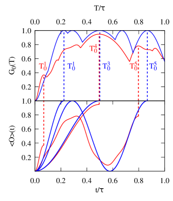
Figure 1: Top: Optimal occupation of the one-photon Fock number state, as a function of the total interaction time $T$ for a weak coupling case ($g\ll\omega$, blue), and an ultrastrong coupling case ($g\approx 0.5\omega$, red). Bottom: Evolution in time of the one-photon Fock number state occupation, when the initial state is optimal for various interaction times $T_{0}^{j}$ corresponding to local maxima of the $G_{0}(T)$ curve. ($j$ indexes the maxima in increasing time order).

IV.2 Creation of $k$-photon Fock states

The same procedure can be used to create Fock states with a larger number of photons. For example, in Fig. 2 we show the results obtained when using the two-photon and three-photon states as targets, i.e.:

$$\hat{O}=\hat{I}_{\rm M}\otimes|k\rangle\langle k|\,,$$ (26)

for $k=2,3$. The plot displays the optimal value attained with varying values of the total interaction time, for several numbers of TLSs. These calculations were performed in the already introduced weak coupling regime.

First, note that the target state is never created with perfect fidelity, in contrast to the one-photon case. However, by increasing $N$, the fidelity grows and reaches values that get arbitrarily close to one. This can be seen by looking for example at the first local maxima of the curves, displayed in the plots with black dots.

One interesting point of those first local maxima is that they somehow generalise the result of the previous section: the optimal initial states of those local maxima are the Dicke states $D(N,k)$, with $k=2$ and 3 excitations for the 2-photon and 3-photon targets, respectively. We observed this fact to hold for larger photonic numbers: the optimal state for the fastest creation of the $k$-photon Fock space is the $D(N,k)$ state, but the state is not created exactly – only in the limit of very large number of TLSs the fidelity can be made arbitrarily close to one.

Finally, the optimal interaction times $T_{0}^{1}(N)$ are also reduced with increasing $N$, following $N^{-1/2}\tau$ trends: $\frac{1}{\sqrt{2}}(N-1)^{-1/2}\tau$ for the 2-photon target, and $\propto(9N-10)^{-1/2}\tau$ for the 3-photon target.

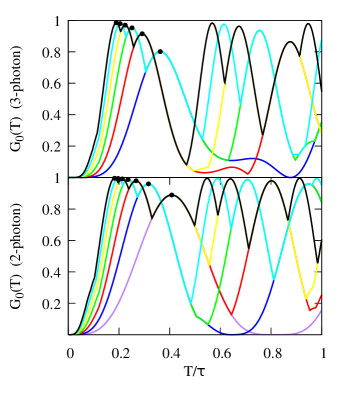
Figure 2: Optimal occupation of the two-photon (top) and three-photon (bottom) Fock number states, as a function of the total interaction time $T$, for various values of the number of TLSs: violet (2), blue (3), red(4), green (5), yellow (6), cyan (7) and black (8). Note that often the curves overlap. The black dots mark the first local maxima.

IV.3 Creation of Dicke states

We now turn to the more familiar problem in the field of QOCT: the attempt to shape an electro-magnetic field such that it induces a given behaviour on a piece of matter, e.g. the preparation of some matter state. Given the special role played by Dicke states when attempting to prepare Fock states, we will set them now as targets for the optimisations. This is achieved by setting the target operator as:

$$\hat{O}=|D(N,k)\rangle\langle D(N,k)|\otimes\hat{I}_{\rm F}\,,$$ (27)

where $\hat{I}_{\rm F}$ is the identity operator in photon space, $N$ is the number of TLSs present in the cavity, and $k$ is the number of excited TLSs in the definition of the state. The TLSs are assumed to be in their ground state at time zero, and therefore the parametrization of the initial state is in this case:

$$|z^{0}(u)\rangle=\sum_{i}^{M}u_{i}\left[|\downarrow\rangle^{\otimes N}\right]\otimes|i\rangle\,,$$ (28)

where $M$ is the cut-off number of photons included in the calculation (a number that we carefully checked to be big enough not to affect the results).

As an example, we display in Fig. 3 the optimisations achieved for the $D(7,k)\;\;(k=1,\dots,7)$ series. The best possible Dicke states will be created at the interaction times that determine the maxima of the curves. Unsurprisingly, the optimal initial states that correspond to the first maxima are, precisely, the Fock number states with $k$ photons. It becomes clear that Fock number states and Dicke states play a “conjugated” role: Fock states are the optimal initial states for the creation of Dicke states, and vice versa.

By looking at the first maxima of the curves one may also note that (i) the fidelity in the production of the Dicke states deteriorates with increasing $k$ – in fact, only the $W$-state ($k=1$) can be created exactly; and (ii) the time needed for the (at least approximate) creation of the Dicke states also becomes longer with increasing $k$. The exception is the $D(7,7)$ state, whose maximum does not correspond to an initial Fock number state but to a linear combination of those, and whose optimal interaction time does not follow the trend of the other cases. The $D(7,7)$ state is indeed peculiar, as it is not an entangled state, but the product of all the TLSs excited states.

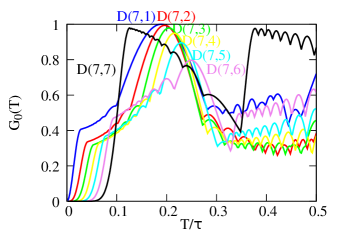
Figure 3: Optimal occupation of the marked Dicke states, as a function of the total interaction time $T$.

IV.4 Multi-mode photon states

The previous examples have assumed a single cavity mode; an obvious generalisation of the Dicke Hamiltonian is the consideration of a number $L$ of radiation modes:

$$\hat{H} = \sum_{n}^{L}\omega_{n}\hat{a}_{n}^{\dagger}\hat{a}_{n}+\frac{1}{2}\sum^{N}_{k}\omega^{(k)}_{0}\hat{\sigma}_{z}$$ (29)

$$+\sum_{n}^{L}\sum_{k}^{N}g_{n}^{(k)}(\hat{a}_{n}^{\dagger}+\hat{a}_{n})(\hat{\sigma}^{(j)}_{+}+\hat{\sigma}^{(+)}_{-})\,.$$

The extra freedom permits to attempt the creation of more complex photon states, such as, if we work with two modes:

$$|R_{1}\rangle=\frac{1}{\sqrt{2}}\left(|10\rangle+|01\rangle\right)\,,$$ (30)

as an example of one-photon state, and, if we work with three modes and two-photon states:

$$|R_{2}\rangle=\frac{1}{\sqrt{2}}\left(|110\rangle+|101\rangle\right)\,.$$ (31)

The corresponding target operators are $\hat{O}=\hat{I}_{M}\otimes|R_{\mu}\rangle\langle R_{\mu}|$ ($\mu=1,2$). The first case involves the presence of (at least) two modes, whereas the second case requires three. The photons occupying these modes are thus entangled – the $R_{1}$ is the prototypical (and controversial) example of single-particle entangled state van Enk (2005); Drezet (2006); van Enk (2006).

In order to successfully couple to those modes, we need to have a number of TLSs resonant to the corresponding frequencies, i.e. some of the $w_{0}^{(k)}$ must be equal to each $\omega_{n}$. We therefore set a number $N_{n}$ of TLSs resonant to each mode ($\sum_{n}N_{n}=N$) and then perform the optimisation using the same procedure as in the previous cases.

The results are shown in Fig. 4. We plot the optimal occupation of the states as a function of the total interaction time $T$, for both targets. For $R_{1}$, the plot shown (blue curve) is the one corresponding to three TLSs per mode ($N_{1}=N_{2}=3$), and it can be seen how there are several optimal times for which the achieved occupation is one. For $R_{2}$ we display two sample calculations, one with two TLSs per mode (red) and one with three (black). It can be seen how the optimal occupations achieved with the latter are higher, and therefore we have the expected trend: the more TLSs, the more freedom in the variational search, and therefore the better the results.

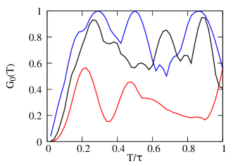
Figure 4: Optimal occupation of the $R_{1}$ as a function of the interaction time $T$ in the presence of three TLS per mode (blue). Optimal occupation of the $R_{2}$ state in the presence of two (red) and three (black) TLSs per mode.

V Conclusions

The machinery of QOCT can be easily extended to include the problem of the optimisation of the initial state of a quantum process such that its evolution produces a pre-defined target outcome – such as the creation of a given state, the maximisation of the projection onto a Hilbert subspace, etc. This idea may be used to generalise the typical QOCT problem – the shaping of an external electromagnetic field in order to control the evolution of a quantum system – to include the case in which the field is no longer external but a part of the system itself. In this case, the shaping must be understood as the preparation of the initial state of the field. Immediately, this idea suggests the complementary concept of shaping the initial state of the matter subsystem in order to control the subsequent evolution of the electromagnetic quantum state.

As in standard QOCT, the method starts with the definition of a target functional. The crucial equations are those of the gradient of this functional with respect to the parameters that define, in this case, the shape of the initial state. The calculation of this gradient essentially requires multiple propagations of the system in time. Therefore, the computational complexity depends on the cost of these propagations. If (1) the target functional is the expectation value of the final state on some operator; (2) the control variables are the expansion coefficients of the initial state in some subspace of allowed initial states; and (3) the quantum evolution equation is the linear Schrödinger equation, then the problem is reduced to the maximisation of a quadratic form, which amounts to the diagonalisation of a matrix whose coefficients are computed by propagation of the basis states.

We have tested these ideas using the Dicke model – a set of TLSs coupled to one radiation mode (or more, in a generalised version) in a cavity. We have examined the creation of Dicke states through the initial preparation of the electromagnetic state, and the creation of Fock radiation states through the initial preparation of the states of the TLSs. Dicke and Fock number states play a conjugated role, as Dicke states turn out to be the optimal initial states for the preparation of Fock number states, and vice versa. The creation of the target states is unfortunately not always exact, and depends on the size of the initial state search subspace – for example, Fock number states are better created if more TLSs are included in the model.

Finally, we outlook a few possible extensions and modifications of this work: (1) First, we note that this reformulation of QOCT is not incompatible with the usual one, as one could have the freedom of shaping both the initial state and an external field – the equations shown above could be trivially extended to include this option. This could be used to guide experimental work in which one has the possibility of both partially preparing the initial state and acting externally on the subsequent evolution. (2) Second, one could take the classical or mean field limit for the electromagnetic field, and consider an OCT formulation for the coupled Maxwell-Schrödinger dynamics. This OCT should therefore target a mixed quantum-classical system, a possibility that has already been realised for models with quantum electrons and classical nuclei Castro and Gross (2014). (3) In this work, the matter subsystem has been modelled with simplified two-level Hamiltonian, but an ab-initio coupled treatment of many-particle systems and photon fields is possible – using, for example, the density functional reformulation of the quantum electrodynamics equations Flick et al. (2015). Work along these three lines is in progress.

Appendix A Derivation of the control equations

The control problem formulated through Eqs. (1-2) and Eq. (4) may be approached through Pontryagin’s principle Boltyanskiĭ et al. (1956); Pontryagin et al. (1962), that establishes a set of necessary conditions for the solution. In essence, the solution must be found at one of the zeros of the gradient of $G$, that is given by:

$$\frac{\partial G}{\partial u_{k}} = \left.\frac{\partial F}{\partial u_{k}}(y(T),u)\right|_{y(T)=y_{u}(T)}+$$ (32)

$$2{\rm Re}\int_{0}^{T}\!\!{\rm d}t\;\langle\lambda_{u}(t)|\left[-{\rm i}\frac{\partial\hat{H}(u,t)}{\partial u_{k}}|y_{u}(t)\rangle+|\frac{\partial b}{\partial u_{k}}(u,t)\rangle\right]$$

In this equation, the costate is defined as the solution to:

$$\dot{\lambda}_{u}(t) = -{\rm i}\hat{H}^{\dagger}(u,t)\lambda_{u}(t)\,,$$ (33)

$$\lambda(T) = \frac{\partial F}{\partial y^{*}}(y_{u}(T),u)\,.$$ (34)

Now we re-consider the reformulation of the problem for the system described through Eqs. (5-6), i.e.:

$$\dot{z}(t) = -{\rm i}\hat{H}z(t)\,,$$ (35)

$$z(0) = z^{0}(u)\,,$$ (36)

for a target function $\tilde{F}(z(T),u)$. Upon the change of variable $y(t)=z(t)-z^{0}(u)$, we get:

$$\dot{y}(t) = -{\rm i}\hat{H}y(t)-{\rm i}\hat{H}z^{0}(u)\,,$$ (37)

$$y(0) = 0\,.$$ (38)

We may therefore use Eq. (32), which results in:

$$\frac{\partial G}{\partial u_{k}} = 2{\rm Re}\langle\frac{\partial\tilde{F}}{\partial z^{*}}(z_{u}(T),u)|\frac{\partial z^{0}}{\partial u_{k}}\rangle+\left.\frac{\partial\tilde{F}}{\partial u_{k}}(z(T),u)\right|_{z(T)=z_{u}(T)}$$ (39)

$$+2{\rm Re}\left[-{\rm i}\int_{0}^{T}\!\!{\rm d}t\;\langle\lambda_{u}(t)|H|\frac{\partial z^{0}}{\partial u_{k}}\rangle\right]\,.$$

Now the costate $\lambda_{u}$ is given by::

$$\lambda_{u}(t)=\hat{U}(t,T)\frac{\partial\tilde{F}}{\partial z^{*}}(z_{u}(T),u)\,.$$ (40)

Therefore:

$$\int_{0}^{T}\!\!{\rm d}t\;\langle\lambda_{u}(t)|H=\int_{0}^{T}\!\!{\rm d}t\;\langle\frac{\partial\tilde{F}}{\partial z^{*}}(z_{u}(T),u)|U(T,t)H$$ (41)

If we use $U(T,t)H=-i\frac{\rm d}{{\rm d}t}U(T,t)$, we finally arrive at:

$$\frac{\partial G}{\partial u_{k}}=\left.\frac{\partial\tilde{F}}{\partial u_{k}}(z(T),u)\right|_{z(T)=z_{u}(T)}+2{\rm Re}\langle\lambda_{u}(0)|\frac{\partial z^{0}}{\partial u_{k}}\rangle\,.$$ (42)

This equation may also be rewritten without any reference to the costate, as in Eq. (10).

References

- Brumer and Shapiro (2003) P. Brumer and M. Shapiro, Principles of the Quantum Control of Molecular Processes (John Wiley, New York, 2003).
- Brif et al. (2010) C. Brif, R. Chakrabarti, and H. Rabitz, New Journal of Physics 12, 075008 (2010).
- Kirk (1998) D. E. Kirk, Optimal Control Theory. An Introduction (Dover Publications, Inc., New York, 1998).
- Walther et al. (2006) H. Walther, B. T. H. Varcoe, B.-G. Englert, and T. Becker, Reports on Progress in Physics 69, 1325 (2006).
- Rojan et al. (2014) K. Rojan, D. M. Reich, I. Dotsenko, J.-M. Raimond, C. P. Koch, and G. Morigi, Phys. Rev. A 90, 023824 (2014).
- Deffner (2014) S. Deffner, Journal of Physics B: Atomic, Molecular and Optical Physics 47, 145502 (2014).
- Allen et al. (2017) J. L. Allen, R. Kosut, J. Joo, P. Leek, and E. Ginossar, Phys. Rev. A 95, 042325 (2017).
- Dicke (1954) R. H. Dicke, Phys. Rev. 93, 99 (1954).
- Garraway (2011) B. M. Garraway, Philosophical Transactions of the Royal Society of London A: Mathematical, Physical and Engineering Sciences 369, 1137 (2011).
- Dür et al. (2000) W. Dür, G. Vidal, and J. I. Cirac, Phys. Rev. A 62, 062314 (2000).
- Werschnik and Gross (2007) J. Werschnik and E. K. U. Gross, J. Phys. B: At. Mol. Opt. Phys. 40, R175 (2007).
- Peirce et al. (1988) A. P. Peirce, M. A. Dahleh, and H. Rabitz, Phys. Rev. A 37, 4950 (1988).
- Tersigni et al. (1990) S. H. Tersigni, P. Gaspard, and S. A. Rice, The Journal of Chemical Physics 93, 1670 (1990).
- Castro et al. (2012) A. Castro, J. Werschnik, and E. K. U. Gross, Phys. Rev. Lett. 109, 153603 (2012).
- Note (1) Note that there is no loss of generality in considering one or the other option: in any numerical implementation of the problem, each function is represented by a set of parameters; inversely, any set of parameters can be considered as a set of functions that are constrained to be constant in time.
- Tavis and Cummings (1968) M. Tavis and F. W. Cummings, Phys. Rev. 170, 379 (1968).
- Tavis and Cummings (1969) M. Tavis and F. W. Cummings, Phys. Rev. 188, 692 (1969).
- Jaynes and Cummings (1963) E. T. Jaynes and F. W. Cummings, Proc. IEEE 51, 89 (1963).
- Shore and Knight (1993) B. W. Shore and P. L. Knight, Journal of Modern Optics 40, 1195 (1993).
- Raimond et al. (2001) J. M. Raimond, M. Brune, and S. Haroche, Rev. Mod. Phys. 73, 565 (2001).
- Meschede et al. (1985) D. Meschede, H. Walther, and G. Müller, Phys. Rev. Lett. 54, 551 (1985).
- Raimond et al. (1982) J. M. Raimond, P. Goy, M. Gross, C. Fabre, and S. Haroche, Phys. Rev. Lett. 49, 117 (1982).
- Agarwal (1998) G. S. Agarwal, Journal of Modern Optics 45, 449 (1998).
- Härkönen et al. (2009) K. Härkönen, F. Plastina, and S. Maniscalco, Phys. Rev. A 80, 033841 (2009).
- Fink et al. (2009) J. M. Fink, R. Bianchetti, M. Baur, M. Göppl, L. Steffen, S. Filipp, P. J. Leek, A. Blais, and A. Wallraff, Phys. Rev. Lett. 103, 083601 (2009).
- França Santos et al. (2001) M. França Santos, E. Solano, and R. L. de Matos Filho, Phys. Rev. Lett. 87, 093601 (2001).
- Bertet et al. (2002) P. Bertet, S. Osnaghi, P. Milman, A. Auffeves, P. Maioli, M. Brune, J. M. Raimond, and S. Haroche, Phys. Rev. Lett. 88, 143601 (2002).
- Brown et al. (2003) K. R. Brown, K. M. Dani, D. M. Stamper-Kurn, and K. B. Whaley, Phys. Rev. A 67, 043818 (2003).
- Zhang et al. (2012) J. Zhang, J. Wang, and T. Zhang, J. Opt. Soc. Am. B 29, 1473 (2012).
- Hofheinz et al. (2008) M. Hofheinz, E. M. Weig, M. Ansmann, R. C. Bialczak, E. Lucero, M. Neeley, A. D. O’Connell, H. Wang, J. M. Martinis, and A. N. Cleland, Nature 454, 310 EP (2008).
- Barnea et al. (2015) T. J. Barnea, G. Pütz, J. B. Brask, N. Brunner, N. Gisin, and Y.-C. Liang, Phys. Rev. A 91, 032108 (2015).
- Wu et al. (2017) C. Wu, C. Guo, Y. Wang, G. Wang, X.-L. Feng, and J.-L. Chen, Phys. Rev. A 95, 013845 (2017).
- van Enk (2005) S. J. van Enk, Phys. Rev. A 72, 064306 (2005).
- Drezet (2006) A. Drezet, Phys. Rev. A 74, 026301 (2006).
- van Enk (2006) S. J. van Enk, Phys. Rev. A 74, 026302 (2006).
- Castro and Gross (2014) A. Castro and E. K. U. Gross, Journal of Physics A: Mathematical and Theoretical 47, 025204 (2014).
- Flick et al. (2015) J. Flick, M. Ruggenthaler, H. Appel, and A. Rubio, Proceedings of the National Academy of Sciences 112, 15285 (2015).
- Boltyanskiĭ et al. (1956) V. G. Boltyanskiĭ, R. V. Gamkrelidze, and L. S. Pontryagin, Dokl. Akad. Nauk SSSR (N.S.) 110, 7 (1956).
- Pontryagin et al. (1962) L. S. Pontryagin, V. G. Boltyanskii, R. V. Gamkrelidze, and E. F. Mishchenko, The Mathematical Theory of Optimal Processes (John Wiley & Sons, 1962).