On compatible linear connections of two-dimensional generalized Berwald manifolds

Abstract.

In the paper we present results about generalized Berwald surfaces involving the intrinsic characterization, some topological obstructions for the base manifold and examples.

In memoriam to V. Wagner on the 75th anniversary of publishing his pioneering work about generalized Berwald manifolds.

Introduction

The concept of generalized Berwald manifolds goes back to V. Wagner [22]. They are Finsler manifolds admitting linear connections such that the parallel transports preserve the Finslerian length of tangent vectors (compatibility condition). To express the compatible linear connection in terms of the canonical data of the Finsler manifold is the problem of the intrinsic characterization we are going to solve in case of two-dimensional generalized Berwald manifolds. The result is formulated in terms of linear inhomogeneous differential equations for the main scalar along the indicatrix curve (Subsection 2.1). As an application we prove that if a Landsberg surface is a generalized Berwald manifold then it must be a Berwald manifold (Subsection 2.2). Especially, we reproduce Wagner’s original result in terms of the conventional setting of Finsler surfaces (Subsection 2.3) in honor of the 75th anniversary of publishing his pioneering work about generalized Berwald manifolds.

The technic of averaging is an alternative way to solve the problem of the characterization of compatible linear connections. By the fundamental result of the theory [15] such a linear connection must be metrical with respect to the averaged Riemannian metric given by integration of the Riemann-Finsler metric on the indicatrix hypersurfaces. Therefore the linear connection is uniquely determined by its torsion tensor. The torsion tensor has a special decomposition in 2D because of

(1) $$T(X,Y)=\left(X^{1}Y^{2}-X^{2}Y^{1}\right)\left(T_{12}^{1}\frac{\partial}{\partial u^{1}}+T_{12}^{2}\frac{\partial}{\partial u^{2}}\right)=\rho(X)Y-\rho(Y)X,$$

where $\rho_{1}=T_{12}^{2}$ and $\rho_{2}=-T_{12}^{1}=T_{21}^{1}$. In higher dimensional spaces such a linear connection is called semi-symmetric. Using some previous results [16], [18], [19] and [20], the torsion tensor of a semi-symmetric compatible linear connection can be expressed in terms of metrics and differential forms given by averaging independently of the dimension of the space. Especially the compatible linear connection must be of zero curvature in 2D unless the manifold is Riemannian, see [21]. Therefore we can conclude some topological obstructions as well due to the divergence representation of the Gauss curvature (Subsection 3.1). We prove, for example, that any compact generalized Berwald surface without boundary must have zero Euler characteristic. Therefore the Euclidean sphere does not carry such a geometric structure. Using the theory of closed Wagner manifolds, this means that the local conformal flatness of the Riemannian surfaces fails for (non-Riemannian) Finslerian ones (Subsection 3.2). We present some examples of non-Riemannian two-dimesnional generalized Berwald manifolds as well (Subsection 3.3).

1. Notations and terminology

Let $M$ be a differentiable manifold with local coordinates $u^{1},\ldots,u^{n}.$ The induced coordinate system of the tangent manifold $TM$ consists of the functions $x^{1},\ldots,x^{n}$ and $y^{1},\ldots,y^{n}$. For any $v\in T_{p}M$, $x^{i}(v)=u^{i}(p)$ and $y^{i}(v)=v(u^{i})$, where $i=1,\ldots,n$ and $\pi\colon TM\to M$ is the canonical projection.

1.1. Finsler metrics

A Finsler metric is a continuous function $F\colon TM\to\mathbb{R}$ satisfying the following conditions:

• $\displaystyle{F}$ is smooth on the complement of the zero section (regularity),

• $\displaystyle{F(tv)=tF(v)}$ for all $\displaystyle{t>0}$ (positive homogenity),

• the Hessian $\displaystyle{g_{ij}=\frac{\partial^{2}E}{\partial y^{i}\partial y^{j}}}$, where $E=\frac{1}{2}F^{2}$ is positive definite at all nonzero elements $\displaystyle{v\in T_{p}M}$ (strong convexity).

The so-called Riemann-Finsler metric $g$ is constituted by the components $g_{ij}$. It is defined on the complement of the zero section. The Riemann-Finsler metric makes each tangent space (except at the origin) a Riemannian manifold with standard canonical objects such as the volume form $\displaystyle{d\mu=\sqrt{\det g_{ij}}\ dy^{1}\wedge\ldots\wedge dy^{n}}$, the Liouville vector field $\displaystyle{C:=y^{1}\partial/\partial y^{1}+\ldots+y^{n}\partial/\partial y^{n}}$ together with its normalized dual form $\displaystyle{l_{i}=\partial F/\partial y^{i}}$ with respect to the Riemann-Finsler metric and the induced volume form

$$\mu=\sqrt{\det g_{ij}}\ \sum_{i=1}^{n}(-1)^{i-1}\frac{y^{i}}{F}dy^{1}\wedge\ldots\wedge dy^{i-1}\wedge dy^{i+1}\ldots\wedge dy^{n}$$

on the indicatrix hypersurface $\displaystyle{\partial K_{p}:=F^{-1}(1)\cap T_{p}M\ \ (p\in M)}$. In what follows we summarize some basic notations. As a general reference of Finsler geometry see [3] and [8]: $\displaystyle{g^{ij}=(g_{ij})^{-1}}$ denotes the inverse of the coefficient matrix of the Riemann-Finsler metric, the (lowered) first Cartan tensor is given by $\displaystyle{C_{ijk}=\frac{1}{2}\partial g_{ij}/\partial y^{k}}$ and $\displaystyle{\mathcal{C}^{l}_{ij}=g^{lk}\mathcal{C}_{ijk}}$. The first Cartan tensor is totally symmetric and $\displaystyle{y^{k}\mathcal{C}_{ijk}=0}$. Its semibasic trace is given by the quantities $\displaystyle{\mathcal{C}_{i}=g^{jk}\mathcal{C}_{ijk}}$ ($i,j,k=1,\ldots,n$). Differentiating $\det g_{ij}$ as a composite function we have that

$$\frac{\partial\det g_{rs}}{\partial y^{i}}=\frac{\partial D}{\ \partial m_{jk}}(M)\frac{\partial g_{jk}}{\partial y^{i}}=(-1)^{j+k}\det\left(M\ \textrm{ without its $j^{th}$ row and $k^{th}$ column}\right)\frac{\partial g_{jk}}{\partial y^{i}}=$$

$$=(\det g_{rs})g^{jk}\frac{\partial g_{jk}}{\partial y^{i}},\ \ \textrm{where}\ \ M:=g_{ij}.$$

Therefore

(2) $$\frac{\partial\ln\sqrt{\det g_{rs}}}{\partial y^{i}}=\frac{1}{2}g^{jk}\frac{\partial g_{jk}}{\partial y^{i}}=g^{jk}\mathcal{C}_{ijk}=\mathcal{C}_{i}.$$

The geodesic spray coefficients and the horizontal sections are

$$G^{l}=\frac{1}{2}g^{lm}\left(y^{k}\frac{\partial^{2}E}{\partial y^{m}\partial x^{k}}-\frac{\partial E}{\partial x^{m}}\right)\ \ \textrm{and}\ \ X_{i}^{h}=\frac{\partial}{\partial x^{i}}-G^{l}_{i}\frac{\partial}{\partial y^{l}},\ \ \textrm{where}\ \ G_{i}^{l}=\frac{\partial G^{l}}{\partial y^{i}}.$$

The second Cartan tensor (Landsberg tensor) and the mixed curvature are given by

$$P^{l}_{ij}=\frac{1}{2}g^{lm}\left(X_{i}^{h}\left(g_{jm}\right)-G^{k}_{ij}g_{km}-G^{k}_{im}g_{jk}\right),\ \ \textrm{where}\ \ G_{ij}^{l}=\frac{\partial G_{i}^{l}}{\partial y^{j}}$$

and $\displaystyle{P_{ijk}^{l}=-G^{l}_{ijk}}$, where $\displaystyle{G_{ijk}^{l}=\frac{\partial G_{ij}^{l}}{\partial y^{k}}}$.

Lemma 1.

(3) $$P^{l}_{ij}=-\frac{F}{2}l_{m}g^{kl}P_{ijk}^{m}$$

Proof. Since

$$Fl_{m}=\frac{\partial E}{\partial y^{m}},\ \ \frac{\partial E}{\partial y^{m}}G^{m}=\frac{1}{2}y^{k}\frac{\partial E}{\partial x^{k}},\ \ g_{mi}G^{m}=\frac{1}{2}\left(y^{k}\frac{\partial^{2}E}{\partial y^{i}\partial x^{k}}-\frac{\partial E}{\partial x^{i}}\right)$$

and

$$\frac{\partial}{\partial y^{i}}\left(\frac{\partial E}{\partial y^{m}}G^{m}\right)-g_{mi}G^{m}=\frac{\partial E}{\partial x^{i}}$$

we have

$$-Fl_{m}P^{m}_{ijk}=\frac{\partial E}{\partial y^{m}}G^{m}_{ijk}=$$

$$\frac{\partial}{\partial y^{k}}\left(\frac{\partial E}{\partial y^{m}}G^{m}_{ij}\right)-g_{mk}G_{ij}^{m}=\frac{\partial}{\partial y^{k}}\left(\frac{\partial}{\partial y^{j}}\left(\frac{\partial E}{\partial y^{m}}G^{m}_{i}\right)-g_{mj}G_{i}^{m}\right)-g_{mk}G_{ij}^{m}=$$

$$\frac{\partial}{\partial y^{k}}\left(\frac{\partial}{\partial y^{j}}\left(\frac{\partial}{\partial y^{i}}\left(\frac{\partial E}{\partial y^{m}}G^{m}\right)-g_{mi}G^{m}\right)-g_{mj}G^{m}_{i}\right)-g_{mk}G_{ij}^{m}=$$

$$\frac{\partial}{\partial y^{k}}\left(\frac{\partial}{\partial y^{j}}\left(\frac{\partial E}{\partial x^{i}}\right)-g_{mj}G^{m}_{i}\right)-g_{mk}G_{ij}^{m}=\frac{\partial}{\partial x^{i}}g_{jk}-2\mathcal{C}_{jmk}G_{i}^{m}-g_{mj}G_{ik}^{m}-g_{mk}G^{m}_{ij}=$$

$$2P_{ijk}=2g_{kl}P^{l}_{ij}\ \ \Rightarrow\ \ P^{l}_{ij}=-\frac{F}{2}l_{m}g^{kl}P_{ijk}^{m}$$

as was to be proved. $\square$

1.2. Generalized Berwald manifolds

Definition 1.

A linear connection $\nabla$ on the base manifold $M$ is called compatible to the Finslerian metric if the parallel transports with respect to $\nabla$ preserve the Finslerian length of tangent vectors. Finsler manifolds admitting compatible linear connections are called generalized Berwald manifolds.

Corollary 1.

A linear connection $\nabla$ on the base manifold $M$ is compatible to the Finslerian metric function if and only if the induced horizontal distribution is conservative, i.e. the derivatives of the fundamental function $F$ vanish along the horizontal directions with respect to $\nabla$.

Proof. Suppose that the parallel transports with respect to $\nabla$ (a linear connection on the base manifold) preserve the Finslerian length of tangent vectors and let $X_{t}$ be a parallel vector field along the curve $c\colon[0,1]\to M$:

(4) $$(x^{k}\circ X_{t})^{\prime}={c^{k}}^{\prime}\ \ \textrm{and}\ \ (y^{k}\circ X_{t})^{\prime}={X_{t}^{k}}^{\prime}=-{c^{i}}^{\prime}X_{t}^{j}\Gamma_{ij}^{k}\circ c$$

because of the differential equation for parallel vector fields. If $F$ is the Finslerian fundamental function then

(5) $$(F\circ X_{t})^{\prime}=(x^{k}\circ X_{t})^{\prime}{\frac{\partial F}{\partial x^{k}}}\circ X_{t}+(y^{k}\circ X_{t})^{\prime}{\frac{\partial F}{\partial y^{k}}}\circ X_{t}$$

and, by formula (4),

(6) $$(F\circ X_{t})^{\prime}={c^{i}}^{\prime}\bigg{(}\frac{\partial F}{\partial x^{i}}-y^{j}{\Gamma}_{ij}^{k}\circ\pi\frac{\partial F}{\partial y^{k}}\bigg{)}\circ X_{t}.$$

This means that the parallel transports with respect to $\nabla$ preserve the Finslerian length of tangent vectors (compatibility condition) if and only if

(7) $$\frac{\partial F}{\partial x^{i}}-y^{j}{\Gamma}^{k}_{ij}\circ\pi\frac{\partial F}{\partial y^{k}}=0\ \ (i=1,\ldots,n),$$

where the vector fields of type

(8) $$\frac{\partial}{\partial x^{i}}-y^{j}{\Gamma}^{k}_{ij}\circ\pi\frac{\partial}{\partial y^{k}}$$

span the associated horizontal distribution belonging to $\nabla$. $\square$

Theorem 1.

[15] If a linear connection on the base manifold is compatible with the Finslerian metric function then it must be metrical with respect to the averaged Riemannian metric

(9) $$\gamma_{p}(v,w):=\int_{\partial K_{p}}g(v,w)\,\mu=v^{i}w^{j}\int_{\partial K_{p}}g_{ij}\,\mu\ \ (v,w\in T_{p}M,p\in U).$$

1.3. Finsler surfaces

In case of Finsler surfaces it is typical to introduce the vector field

$$V:=\frac{\partial F}{\partial y^{1}}\frac{\partial}{\partial y^{2}}-\frac{\partial F}{\partial y^{2}}\frac{\partial}{\partial y^{1}}.$$

It is tangential to the indicatrix curve because of $VF=0$. Since three vertical vector fields must be linearly dependent in 2D,

$$0=\det\left(\begin{array}[]{ccc}g\left(\frac{\partial}{\partial y^{1}},\frac{\partial}{\partial y^{1}}\right)&g\left(\frac{\partial}{\partial y^{1}},\frac{\partial}{\partial y^{2}}\right)&g\left(\frac{\partial}{\partial y^{1}},C\right)\\ &&\\ g\left(\frac{\partial}{\partial y^{2}},\frac{\partial}{\partial y^{1}}\right)&g\left(\frac{\partial}{\partial y^{2}},\frac{\partial}{\partial y^{2}}\right)&g\left(\frac{\partial}{\partial y^{2}},C\right)\\ &&\\ g\left(C,\frac{\partial}{\partial y^{1}}\right)&g\left(C,\frac{\partial}{\partial y^{2}}\right)&g\left(C,C\right)\\ &&\\ \end{array}\right)=\det\left(\begin{array}[]{ccc}g_{11}&g_{12}&\partial E/\partial y^{1}\\ &&\\ g_{12}&g_{22}&\partial E/\partial y^{2}\\ &&\\ \partial E/\partial y^{1}&\partial E/\partial y^{2}&2E\\ &&\\ \end{array}\right)=$$

$$F^{2}\det g_{ij}+2g_{12}\frac{\partial E}{\partial y^{1}}\frac{\partial E}{\partial y^{2}}-\left(\frac{\partial E}{\partial y^{1}}\right)^{2}g_{22}-\left(\frac{\partial E}{\partial y^{2}}\right)^{2}g_{11}=F^{2}\left(\det g_{ij}-g(V,V)\right).$$

This means that $\displaystyle{0\neq\det g_{ij}=g(V,V)}$ and, consequently,

$$V_{0}:=\frac{1}{\sqrt{g(V,V)}}V,\ \ C_{0}:=\frac{1}{F}C,\ \ V_{0}^{h}:=V_{0}^{i}X_{i}^{h}=V_{0}^{i}\left(\frac{\partial}{\partial x^{i}}-G^{l}_{i}\frac{\partial}{\partial y^{l}}\right),\ \ S_{0}:=\frac{1}{F}S=\frac{y^{i}}{F}X_{i}^{h}$$

form a local frame on the complement of the zero section in $\pi^{-1}(U)$. Such a collection of vector fields is called a Berwald frame on the tangent manifold.

Definition 2.

The main scalar of a Finsler surface is defined as $\displaystyle{\lambda:=V_{0}^{j}V_{0}^{k}V_{0}^{l}\mathcal{C}_{jkl}},$ where $\displaystyle{V_{0}=V/\sqrt{g(V,V)}}$ is the unit tangential vector field to the indicatrix curve.

The vanishing of the main scalar implies that the surface is Riemannian and vice versa. The zero homogeneous version $I:=F\lambda$ of the main scalar is also frequently used in the literature [4], [5], [6] and [8]. Consider the vector field $\displaystyle{\mathcal{C}^{k}_{ij}\partial/\partial y^{k}}$. Since it is also tangential to the indicatrix surface it follows that

$$\mathcal{C}^{k}_{ij}\frac{\partial}{\partial y^{k}}=\mathcal{C}^{l}_{ij}g\left(V_{0},\frac{\partial}{\partial y^{l}}\right)V_{0},$$

where $\displaystyle{V_{0}=V/\sqrt{g(V,V)}}$ is the unit tangential vector field to the indicatrix curve. Therefore

$$\mathcal{C}^{k}_{ij}=\mathcal{C}^{l}_{ij}g_{lm}V_{0}^{m}V_{0}^{k}=V_{0}^{m}\mathcal{C}_{ijm}V_{0}^{k}\ \ \Rightarrow\ \ \mathcal{C}_{ijr}=V_{0}^{m}\mathcal{C}_{ijm}V_{0}^{k}g_{kr}.$$

Contracting by $g^{rj}$

(10) $$\mathcal{C}_{i}=V_{0}^{j}V_{0}^{m}\mathcal{C}_{ijm}.$$

By formulas (2) and (10) we have that

(11) $$\lambda:=V_{0}^{j}V_{0}^{k}V_{0}^{l}\mathcal{C}_{jkl}=V_{0}^{j}\mathcal{C}_{j}=V_{0}\left(\ln\sqrt{\det g_{rs}}.\right)$$

In what follows we summarize some of the general formulas to express the surviving components of the Landsberg tensor, the mixed curvature tensor and the pairwise Lie-brackets of a Berwald frame (Cartan’s permutation formulas) [12]:

(12) $$y^{i}V_{0}^{j}V_{0}^{k}P_{ijk}=y^{i}V_{0}^{j}V_{0}^{k}G^{l}_{ijk}g\left(V_{0},\frac{\partial}{\partial y^{l}}\right)=0,$$

$$V_{0}^{i}V_{0}^{j}V_{0}^{k}P_{ijk}=-S(\lambda),\ \ V_{0}^{i}V_{0}^{j}V_{0}^{k}G^{l}_{ijk}g\left(V_{0},\frac{\partial}{\partial y^{l}}\right)=V_{0}^{h}(\lambda)+V_{0}(S\lambda)$$

because of the homogenity properties; see [12, Corollary 1.8.] and [12, Formula (24a)]. E. Cartan’s permutation formulas are

(13) $$[V_{0},V_{0}^{h}]=-\frac{1}{F}S_{0}-\lambda V_{0}^{h}-S(\lambda)V_{0},\ \ [S_{0},V_{0}]=-\frac{1}{F}V_{0}^{h},\ \ [V_{0}^{h},S_{0}]=-\kappa V_{0},$$

where $\kappa$ is the only surviving coefficient of the curvature of the horizontal distribution [12, Theorem 1.10]. Let the indicatrix curve in $T_{p}M$ be parameterized as the integral curve of $V_{0}$:

$$V_{0}\circ c_{p}(\theta)=c_{p}^{\prime}(\theta)\ \ \Rightarrow\ \ \lambda\circ c_{p}(\theta)=\left(\ln\sqrt{\det g_{rs}}\circ c_{p}\right)^{\prime}(\theta).$$

It is called the central affine arcwise parametrization of the indicatrix curve. The parameter $\theta$ is ”the central affine length of the arc of the indicatrix” and the main scalar can be interpreted as its ”central affine curvature”; for the citations see [22].

2. Two-dimensional generalized Berwald manifolds

Let $\nabla$ be a linear connection on the base manifold $M$ and suppose that the parallel transports preserve the Finslerian length of tangent vectors (compatibility condition). By Corollary 1,

$$\frac{\partial E}{\partial x^{i}}-y^{m}\Gamma_{im}^{l}\circ\pi\frac{\partial E}{\partial y^{l}}=0\ \ (i=1,2).$$

2.1. The comparison of $\nabla$ with the canonical horizontal distribution of the Finsler manifold

Using the canonical horizontal sections we can write that

$$y^{m}\Gamma_{im}^{l}\circ\pi\frac{\partial E}{\partial y^{l}}-G^{l}_{i}\frac{\partial E}{\partial y^{l}}=0.$$

Since the vertical vector fields are the linear combinations of $V$ and $C$, it follows that

$$y^{m}\Gamma_{im}^{l}\circ\pi\frac{\partial}{\partial y^{l}}-G^{l}_{i}\frac{\partial}{\partial y^{l}}=f_{i}V+g_{i}C\ \ (i=1,2);$$

the coefficients $f_{1}$, $f_{2}$ are positively homogeneous of degree one, $g_{1}$ and $g_{2}$ are positively homogeneous of degree zero. Since $VE=0$ but $CE=2E$, we have that $g_{1}=g_{2}=0$ and, consequently

(14) $$y^{m}\Gamma_{im}^{l}\circ\pi\frac{\partial}{\partial y^{l}}-G^{l}_{i}\frac{\partial}{\partial y^{l}}=f_{i}V\ \ \Rightarrow\ \ y^{m}\Gamma_{im}^{k}\circ\pi\frac{\partial}{\partial y^{k}}=G^{k}_{i}\frac{\partial}{\partial y^{k}}+f_{i}V\ \ (i=1,2).$$

To provide the linearity of the right hand side we should take the Lie brackets with the vertical coordinate vector fields two times:

$$0=\left[\left[y^{m}\Gamma_{im}^{l}\circ\pi\frac{\partial}{\partial y^{l}},\frac{\partial}{\partial y^{j}}\right],\frac{\partial}{\partial y^{k}}\right]=\left[\left[G^{l}_{i}\frac{\partial}{\partial y^{l}},\frac{\partial}{\partial y^{j}}\right],\frac{\partial}{\partial y^{k}}\right]+\left[\left[f_{i}V,\frac{\partial}{\partial y^{j}}\right],\frac{\partial}{\partial y^{k}}\right]=$$

$$G_{ijk}^{l}\frac{\partial}{\partial y^{l}}+f_{i}\left[\left[V,\frac{\partial}{\partial y^{j}}\right],\frac{\partial}{\partial y^{k}}\right]-\frac{\partial f_{i}}{\partial y^{j}}\left[V,\frac{\partial}{\partial y^{k}}\right]-\frac{\partial f_{i}}{\partial y^{k}}\left[V,\frac{\partial}{\partial y^{j}}\right]+\frac{\partial^{2}f_{i}}{\partial y^{j}\partial y^{k}}V=:W_{ijk},$$

where

$$\left[V,\frac{\partial}{\partial y^{j}}\right]=\frac{\partial^{2}F}{\partial y^{j}\partial y^{2}}\frac{\partial}{\partial y^{1}}-\frac{\partial^{2}F}{\partial y^{j}\partial y^{1}}\frac{\partial}{\partial y^{2}},\ \ \left[\left[V,\frac{\partial}{\partial y^{j}}\right],\frac{\partial}{\partial y^{k}}\right]=-\frac{\partial^{3}F}{\partial y^{j}\partial y^{k}\partial y^{2}}\frac{\partial}{\partial y^{1}}+\frac{\partial^{3}F}{\partial y^{j}\partial y^{k}\partial y^{1}}\frac{\partial}{\partial y^{2}}.$$

Since $\displaystyle{y^{j}W_{ijk}=y^{k}W_{ijk}=0}$ it is enough to investigate the quantity $W_{i}=V^{j}V^{k}W_{ijk}$. By some direct computations

$$V^{j}\frac{\partial^{2}F}{\partial y^{j}\partial y^{2}}=V\left(\frac{\partial F}{\partial y^{2}}\right)=\frac{1}{F}V\left(F\frac{\partial F}{\partial y^{2}}\right)=\frac{1}{F}g\left(V,\frac{\partial}{\partial y^{2}}\right)$$

because of $VF=0$. On the other hand

$$V^{j}V^{k}\frac{\partial^{3}F}{\partial y^{j}\partial y^{k}\partial y^{2}}=\frac{1}{F}V^{k}V\left(F\frac{\partial^{2}F}{\partial y^{k}\partial y^{2}}\right)=\frac{1}{F}V^{k}V\left(g_{k2}-\frac{\partial F}{\partial y^{k}}\frac{\partial F}{\partial y^{2}}\right)=$$

$$\frac{1}{F}\left(2V^{j}V^{k}\mathcal{C}_{jk2}-V^{k}V\left(\frac{\partial F}{\partial y^{k}}\right)\frac{\partial F}{\partial y^{2}}\right)=\frac{1}{F}\left(2V^{j}V^{k}\mathcal{C}_{jk2}-\frac{1}{F}V^{k}V\left(F\frac{\partial F}{\partial y^{k}}\right)\frac{\partial F}{\partial y^{2}}\right)=$$

$$\frac{1}{F}\left(2V^{j}V^{k}\mathcal{C}_{jk2}-\frac{1}{F}g(V,V)\frac{\partial F}{\partial y^{2}}\right)$$

and, consequently,

$$W_{i}=V^{j}V^{k}G_{ijk}^{l}\frac{\partial}{\partial y^{l}}-\frac{2V(f_{i})}{F}\left(g\left(V,\frac{\partial}{\partial y^{2}}\right)\frac{\partial}{\partial y^{1}}-g\left(V,\frac{\partial}{\partial y^{1}}\right)\frac{\partial}{\partial y^{2}}\right)-$$

(15) $$\frac{f_{i}}{F}\left(\left(2V^{j}V^{k}\mathcal{C}_{jk2}-\frac{1}{F}g(V,V)\frac{\partial F}{\partial y^{2}}\right)\frac{\partial}{\partial y^{1}}-\left(2V^{j}V^{k}\mathcal{C}_{jk1}-\frac{1}{F}g(V,V)\frac{\partial F}{\partial y^{1}}\right)\frac{\partial}{\partial y^{2}}\right)+$$

$$V^{j}V^{k}\frac{\partial^{2}f_{i}}{\partial y^{j}\partial y^{k}}V.$$

The vanishing of $W_{i}$ is equivalent to

(16) $$g(W_{i},V_{0})=0\ \ \textrm{and}\ \ g(W_{i},C_{0})=0\ \ (i=1,2),$$

where $V_{0}=V/\sqrt{g(V,V)}$ and $C_{0}=C/F$ are the normalized vector fields of the vertical Berwald frame.

2.1.1. The vanishing of the orthogonal term to the indicatrix

It follows that

$$0=g(W_{i},C)=W_{i}E=FV^{j}V^{k}G_{ijk}^{l}\frac{\partial F}{\partial y^{l}}-2V(f_{i})g(V,V)-2f_{i}V^{j}V^{k}V^{l}\mathcal{C}_{jkl}.$$

Therefore

(17) $$\frac{\alpha_{i}}{\sqrt{g(V,V)}}=\lambda f_{i}+\left(V_{0}f_{i}\right)\ \ (i=1,2),$$

where $V_{0}=V/\sqrt{g(V,V)}$ is the unit tangential vector field to the indicatrix curve, $\lambda$ is the main scalar and

$$\alpha_{i}=\frac{1}{2}FV_{0}^{j}V_{0}^{k}G_{ijk}^{l}\frac{\partial F}{\partial y^{l}}\stackrel{{\scriptstyle(\ref{eq:4})}}{{=}}V_{0}^{j}V_{0}^{k}P_{ijk}.$$

Using that $\displaystyle{\det g_{ij}=g(V,V)}$, formula (11) says that

(18) $$\alpha_{i}=V_{0}\left(f_{i}\sqrt{g(V,V)}\right)\ \ (i=1,2).$$

Let the indicatrix curve $c_{p}$ in $T_{p}M$ be parameterized as the integral curve of $V_{0}$. Evaluating along $c_{p}$ we have

(19) $$\alpha_{i}\circ c_{p}(\theta)=\left(f_{i}\circ c_{p}\sqrt{g(V,V)}\circ c_{p}\right)^{\prime}(\theta)\ \ (i=1,2)$$

for any $p\in U$. Therefore

(20) $$\beta_{i}\circ c_{p}(t)=f_{i}\circ c_{p}(t)\sqrt{g(V,V)}\circ c_{p}(t)-f_{i}\circ c_{p}(0)\sqrt{g(V,V)}\circ c_{p}(0),$$

where $\displaystyle{\beta_{i}\colon\pi^{-1}(U)\to\mathbb{R}}$ $(i=1,2)$ are the $1$-homogeneous extensions of the functions defined by

(21) $$\beta_{i}\circ c_{p}(t)=\int_{0}^{t}\alpha_{i}\circ c_{p}(\theta)\,d\theta\ \ (i=1,2)$$

along the central affine arcwise parametrization of the indicatrix curve. We can write that

(22) $$f_{i}\circ c_{p}(t)=\frac{1}{\sqrt{g(V,V)}\circ c_{p}(t)}\left(\beta_{i}\circ c_{p}(t)+k_{i}(p)\right)\ \ (i=1,2)$$

for some constants $k_{i}(p)$ ($i=1,2$) depending only on the position.

2.1.2. The vanishing of the tangential term to the indicatrix

It follows that

$$0=g(W_{i},V)=V^{j}V^{k}G^{l}_{ijk}g\left(V,\frac{\partial}{\partial y^{l}}\right)-\frac{2f_{i}}{F}\left(V^{j}V^{k}\mathcal{C}_{jk2}g\left(V,\frac{\partial}{\partial y^{1}}\right)-V^{j}V^{k}\mathcal{C}_{jk1}g\left(V,\frac{\partial}{\partial y^{2}}\right)\right)+$$

$$\frac{f_{i}}{F^{2}}g(V,V)\left(\frac{\partial F}{\partial y^{2}}g\left(V,\frac{\partial}{\partial y^{1}}\right)-\frac{\partial F}{\partial y^{1}}g\left(V,\frac{\partial}{\partial y^{2}}\right)\right)+V^{j}V^{k}\frac{\partial^{2}f_{i}}{\partial y^{j}\partial y^{k}}g(V,V)=V^{j}V^{k}G^{l}_{ijk}g\left(V,\frac{\partial}{\partial y^{l}}\right)$$

$$+V^{j}V^{k}\frac{\partial^{2}f_{i}}{\partial y^{j}\partial y^{k}}g(V,V)-\frac{f_{i}}{F^{2}}g^{2}(V,V)-\frac{2f_{i}}{F}\left(V^{j}V^{k}\mathcal{C}_{jk2}g\left(V,\frac{\partial}{\partial y^{1}}\right)-V^{j}V^{k}\mathcal{C}_{jk1}g\left(V,\frac{\partial}{\partial y^{2}}\right)\right),$$

where

$$V^{j}V^{k}\mathcal{C}_{jk2}g\left(V,\frac{\partial}{\partial y^{1}}\right)-V^{j}V^{k}\mathcal{C}_{jk1}g\left(V,\frac{\partial}{\partial y^{2}}\right)=0$$

because the vector field

$$Z:=g\left(V,\frac{\partial}{\partial y^{1}}\right)\frac{\partial}{\partial y^{2}}-g\left(V,\frac{\partial}{\partial y^{2}}\right)\frac{\partial}{\partial y^{1}}$$

is parallel to $C$, i.e. $\displaystyle{g(V,Z)=0}$. Therefore

$$0=V^{j}V^{k}G^{l}_{ijk}g\left(V,\frac{\partial}{\partial y^{l}}\right)+V^{j}V^{k}\frac{\partial^{2}f_{i}}{\partial y^{j}\partial y^{k}}g(V,V)-\frac{f_{i}}{F^{2}}g^{2}(V,V)$$

and, consequently,

(23) $$0=V_{0}^{j}V_{0}^{k}G^{l}_{ijk}g\left(V_{0},\frac{\partial}{\partial y^{l}}\right)+V_{0}^{j}V_{0}^{k}\frac{\partial^{2}f_{i}}{\partial y^{j}\partial y^{k}}\sqrt{g(V,V)}-\frac{f_{i}}{F^{2}}\sqrt{g(V,V)}.$$

Lemma 2.

If $g$ is a positively homogeneous function of degree $k$, then

(24) $$V_{0}(V^{k}_{0})\frac{\partial g}{\partial y^{k}}=-\lambda V_{0}(g)-k\frac{g}{F^{2}}.$$

Especially,

(25) $$V_{0}^{j}V_{0}^{k}\frac{\partial^{2}f_{i}}{\partial y^{j}\partial y^{k}}=V_{0}(V_{0}f_{i})+\lambda V_{0}(f_{i})+\frac{f_{i}}{F^{2}}.$$

Proof. Let $c_{p}$ be the parametrization of the indicatrix curve in $T_{p}M$ as the integral curve of $V_{0}$, i.e. $V_{0}\circ c_{p}=c_{p}^{\prime}$. Differentiating equation

(26) $$1=g_{c_{p}}(V_{0}\circ c_{p},V_{0}\circ c_{p})=g_{ij}\circ c_{p}(c_{p}^{i})^{\prime}(c_{p}^{j})^{\prime}$$

we have that $\displaystyle{0=2g_{ij}\circ c_{p}(c^{i}_{p})^{\prime\prime}(c^{j}_{p})^{\prime}+2\mathcal{C}_{ijk}\circ c_{p}(c_{p}^{i})^{\prime}(c_{p}^{j})^{\prime}(c_{p}^{k})^{\prime}}$ and, consequently,

(27) $$g_{c_{p}}(V_{0}\circ c_{p},c_{p}^{\prime\prime})=g_{c_{p}}(c_{p}^{\prime},c_{p}^{\prime\prime})=-\mathcal{C}_{ijk}\circ c_{p}(c_{p}^{i})^{\prime}(c_{p}^{j})^{\prime}(c_{p}^{k})^{\prime}=-\left(V_{0}^{i}V_{0}^{j}V_{0}^{k}\mathcal{C}_{ijk}\right)\circ c_{p}=-\lambda\circ c_{p}.$$

Differentiating equation

(28) $$0=g_{c_{p}}(C\circ c_{p},V_{0}\circ c_{p})=g_{ij}\circ c_{p}(c^{i}_{p})(c_{p}^{j})^{\prime}$$

we have that

(29) $$0=2\mathcal{C}_{ijk}\circ c_{p}(c^{i}_{p})(c_{p}^{j})^{\prime}(c_{p}^{k})^{\prime}+g_{ij}\circ c_{p}(c_{p}^{i})^{\prime}(c_{p}^{j})^{\prime}+g_{ij}\circ c_{p}(c_{p})^{i}(c_{p}^{j})^{\prime\prime}.$$

Taking into account that $\displaystyle{\mathcal{C}_{ijk}\circ c_{p}(c^{i}_{p})(c_{p}^{j})^{\prime}(c_{p}^{k})^{\prime}=\mathcal{C}_{ijk}\circ c_{p}(y^{i}\circ c_{p})(c_{p}^{j})^{\prime}(c_{p}^{k})^{\prime}=0}$,

$$g_{ij}\circ c_{p}(c_{p}^{i})^{\prime}(c_{p}^{j})^{\prime}=g_{c_{p}}(c_{p}^{\prime},c_{p}^{\prime})=1\ \ \textrm{and}\ \ g_{ij}\circ c_{p}(c_{p})^{i}(c_{p}^{j})^{\prime\prime}=g_{c_{p}}(C\circ c_{p},c^{{}^{\prime\prime}}_{p}),$$

it follows that

(30) $$g_{c_{p}}(C_{0}\circ c_{p},c^{{}^{\prime\prime}}_{p})=-\frac{1}{F\circ c_{p}},$$

where $C_{0}:=C/F$ is the normalized Liouville vector field. From (27) and (30)

(31) $$c^{{}^{\prime\prime}}_{p}=-(\lambda V_{0})\circ c_{p}-\frac{1}{F\circ c_{p}}C_{0}\circ c_{p}.$$

This means that

$$\left(V_{0}(V^{k}_{0})\frac{\partial g}{\partial y^{k}}\right)\circ c_{p}=(V^{k}_{0}\circ c_{p})^{\prime}\frac{\partial g}{\partial y^{k}}\circ c_{p}=(c_{p}^{k})^{\prime\prime}\frac{\partial g}{\partial y^{k}}\circ c_{p}\overset{(\ref{curve4})}{=}$$

$$-\left((\lambda V^{k}_{0})\circ c_{p}+\frac{1}{F\circ c_{p}}C^{k}_{0}\circ c_{p}\right)\frac{\partial g}{\partial y^{k}}\circ c_{p}=-(\lambda V_{0}g)\circ c_{p}-\frac{1}{F^{2}\circ c_{p}}(Cg)\circ c_{p},$$

where $\displaystyle{Cg=kg}$ because of the homogenity. Note that the terms $\displaystyle{V_{0}(V^{k}_{0})\partial g/\partial y^{k}}$, $\displaystyle{\lambda V^{k}_{0}g}$ and $\displaystyle{g/F^{2}}$ are of the same degree of homogenity, i.e. they are homogeneous of degree $k-2$. Therefore the equality along the indicatrix curve implies (24). Especially,

$$V_{0}(V_{0}f_{i})=V_{0}^{j}V_{0}^{k}\frac{\partial^{2}f_{i}}{\partial y^{j}\partial y^{k}}+V_{0}(V^{k}_{0})\frac{\partial f_{i}}{\partial y^{k}}=V_{0}^{j}V_{0}^{k}\frac{\partial^{2}f_{i}}{\partial y^{j}\partial y^{k}}-\lambda V_{0}(f_{i})-\frac{f_{i}}{F^{2}}$$

as was to be proved. $\square$

Using Lemma 2 we can write formula (23) into the form

(32) $$0=\omega_{i}+\left(V_{0}(V_{0}f_{i})\right)\sqrt{g(V,V)}+\lambda V_{0}(f_{i})\sqrt{g(V,V)},$$

where

$$\omega_{i}=V_{0}^{j}V_{0}^{k}G^{l}_{ijk}g\left(V_{0},\frac{\partial}{\partial y^{l}}\right)\ \ (i=1,2).$$

By formula (11)

(33) $$0=\omega_{i}+\left(V_{0}(V_{0}f_{i})\right)\sqrt{g(V,V)}+V_{0}(f_{i})V_{0}\left(\sqrt{g(V,V)}\right)\ \ (i=1,2)$$

because of $\displaystyle{\det g_{ij}=g(V,V)}$. Therefore

(34) $$0=\omega_{i}+V_{0}\left((V_{0}f_{i})\sqrt{g(V,V)}\right),$$

(35) $$0=\omega_{i}+V_{0}\left(V_{0}\left(f_{i}\sqrt{g(V,V)}\right)-f_{i}V_{0}\left(\sqrt{g(V,V)}\right)\right),$$

(36) $$0=\omega_{i}+V_{0}\left(V_{0}\left(f_{i}\sqrt{g(V,V)}\right)-\lambda f_{i}\sqrt{g(V,V)}\right),$$

(37) $$0=\omega_{i}+V_{0}\left(V_{0}\left(f_{i}\sqrt{g(V,V)}\right)\right)-V_{0}(\lambda)f_{i}\sqrt{g(V,V)}-\lambda V_{0}\left(f_{i}\sqrt{g(V,V)}\right)\ \ (i=1,2).$$

By formula (18)

(38) $$0=\omega_{i}+V_{0}\left(\alpha_{i}\right)-V_{0}(\lambda)f_{i}\sqrt{g(V,V)}-\lambda\alpha_{i}\ \ (i=1,2).$$

Evaluating formula (38) along $c_{p}$

(39) $$\omega_{i}\circ c_{p}(t)+(\alpha_{i}\circ c_{p})^{\prime}(t)=\left(\beta_{i}\circ c_{p}(t)+k_{i}(p)\right)(\lambda\circ c_{p})^{\prime}(t)+\lambda\circ c_{p}(t)\alpha_{i}\circ c_{p}(t)\ \ (i=1,2)$$

because of (21) and (22). The constants $k_{1}(p)$ and $k_{2}(p)$ of integration can be expressed by (39) provided that $\displaystyle{\lambda\circ c_{p}}$ is not a constant function:

$$k_{i}(p)=\frac{\gamma_{i}\circ c_{p}(s)-\beta_{i}\circ c_{p}(s)\lambda\circ c_{p}(s)+\alpha_{i}\circ c_{p}(s)-\alpha_{i}\circ c_{p}(0)}{\lambda\circ c_{p}(s)-\lambda\circ c_{p}(0)},$$

where

$$\gamma_{i}\circ c_{p}(s)=\int_{0}^{s}\omega_{i}\circ c_{p}(t)\,dt\ \ (i=1,2)$$

and the parameter $s\in\mathbb{R}$ is choosen such that $\displaystyle{\lambda\circ c_{p}(s)-\lambda\circ c_{p}(0)\neq 0}$. Otherwise the function $\displaystyle{\lambda\circ c_{p}}$ is constant. Since $\det g_{ij}$ attains its extremals along the indicatrix curve, formula (11) shows that $\displaystyle{\lambda\circ c_{p}}$ is identically zero and the indicatrix is a quadratic curve in $T_{p}M$. The quadratic indicatrix curve of a (connected) generalized Berwald manifold at a single point implies that the indicatrices are quadratic curves at any point and we have a Riemannian surface. Indeed, the parallel transports induced by the compatible linear connection take a quadratic curve into quadratic curves.

Theorem 2.

The compatible linear connection of a non-Riemannian connected generalized Berwald surface must be of the form

(40) $$\Gamma_{ij}^{1}\circ\pi=G^{1}_{ij}-\frac{\partial f_{i}}{\partial y^{j}}\frac{\partial F}{\partial y^{2}}-f_{i}\frac{\partial^{2}F}{\partial y^{j}\partial y^{2}},\ \ \Gamma_{ij}^{2}\circ\pi=G^{2}_{ij}+\frac{\partial f_{i}}{\partial y^{j}}\frac{\partial F}{\partial y^{1}}+f_{i}\frac{\partial^{2}F}{\partial y^{j}\partial y^{1}}\ \ (i,j=1,2),$$

where the functions $f_{1}$, $f_{2}$ are given by

(41) $$f_{i}\circ c_{p}(t)=\frac{1}{\sqrt{g(V,V)}\circ c_{p}(t)}\left(\int_{0}^{t}\alpha_{i}\circ c_{p}(\theta)\,d\theta+k_{i}(p)\right)\ \ (i=1,2)$$

and the integration constants satisfy equations

(42) $$\omega_{i}\circ c_{p}(t)+(\alpha_{i}\circ c_{p})^{\prime}(t)=\left(\int_{0}^{t}\alpha_{i}\circ c_{p}(\theta)\,d\theta+k_{i}(p)\right)(\lambda\circ c_{p})^{\prime}(t)+\lambda\circ c_{p}(t)\alpha_{i}\circ c_{p}(t)\ \ (i=1,2)$$

for any $p\in M$.

Proof. Equations for the functions $f_{1}$ and $f_{2}$ imply that $g(W_{i},C)=0$ because of subsection 2.1.1. Equations for the integration constants imply that $\displaystyle{g(W_{i},V_{0})=0}$ because of subsection 2.1.2. Therefore $W_{i}=0$ and we have a generalized Berwald surface. The explicite formulas for the coefficients of the linear connection preserving the Finslerian length of tangent vectors are

(43) $$\Gamma_{ij}^{1}\circ\pi=G^{1}_{ij}+\frac{\partial f_{i}}{\partial y^{j}}V^{1}-f_{i}\frac{\partial^{2}F}{\partial y^{j}\partial y^{2}},\ \ \Gamma_{ij}^{2}\circ\pi=G^{2}_{ij}+\frac{\partial f_{i}}{\partial y^{j}}V^{2}+f_{i}\frac{\partial^{2}F}{\partial y^{j}\partial y^{1}}\ \ (i,j=1,2),$$

because of formula (14). $\square$

Corollary 2.

The compatible linear connection of a generalized Berwalds surface is uniquely determined.

2.2. An application: Landsberg and generalized Berwald surfaces

Definition 3.

A Finsler manifold is called a Landsberg manifold if the Landsberg tensor of the canonical horizontal distribution vanishes. The Berwald manifolds are defined by the vanishing of the mixed curvature tensor of the canonical horizontal distribution.

Formula (3) implies that any Berwald manifold is a Landsberg manifold. The converse of this statement is the famous Unicorn problem in Finsler geometry [2].

Theorem 3.

A connected non-Riemannian two-dimensional generalized Berwald surface is a Landsberg surface if and only if it is a Berwald surface.

Proof. Suppose that we have a connected non-Riemannian two-dimensional generalized Berwald manifold such that the Landsberg tensor vanishes, i.e. $\alpha_{i}=0$ ($i=1,2$). Then (22) implies that

(44) $$f_{i}\sqrt{g(V,V)}=k_{i}(p)F$$

for any point $p\in M$. On the other hand

(45) $$\omega_{i}-V_{0}(\lambda)f_{i}\sqrt{g(V,V)}=0$$

due to (38). Contracting by $y^{i}$

(46) $$V_{0}(\lambda)y^{i}k_{i}(p)=0.$$

If there exists a point $p\in M$ such that $\displaystyle{k_{1}^{2}(p)+k_{2}^{2}(p)\neq 0.}$ then $\displaystyle{y^{1}k_{1}(p)+y^{2}k_{2}(p)=0}$ is an equation of a line in $T_{p}M$. Therefore, there are at most two positions along $\partial K_{p}$ such that $\displaystyle{v^{1}k_{1}(p)+v^{2}k_{2}(p)=0}$. Otherwise $V_{0}(v)\lambda=0$ because of (46). A continuity argument says that $V_{0}(v)\lambda=0$ for any $v\in T_{p}M$, i.e. $\lambda$ is constant along $c_{p}$. Since $\det g_{ij}$ attains its extremals along the indicatrix curve, formula (11) shows that $\lambda\circ c_{p}=0$. This means that the indicatrix is a quadratic curve in $T_{p}M$. The quadratic indicatrix curve of a (connected) generalized Berwald manifold at a single point implies that the indicatrices are quadratic curves at any point due to the compatible linear connection and the induced linear mapping between the tangent spaces. This is a contradiction because the generalized Berwald surface is non-Riemannian. Otherwise $\displaystyle{k_{1}(p)=k_{2}(p)=0}$ for any $p\in M$, i.e. $f_{i}=0$ ($i=1,2$) and the compatible linear connection must be the canonical one. Therefore we have a Berwald manifold. $\square$

2.3. Wagner’s equations

To present Wagner’s equations in [22] we need the following simple observation:

$$H_{i}=0\ \ (i=1,2)\ \ \textrm{if and only if}\ \ y^{i}H_{i}=0\ \ \textrm{and}\ \ V_{0}^{i}H_{i}=0$$

because of

$$\det\left(\begin{array}[]{cc}y^{1}&y^{2}\\ V_{0}^{1}&V_{0}^{2}\\ \end{array}\right)=y^{1}V_{0}^{2}-y^{2}V_{0}^{1}=\frac{F}{\sqrt{g(V,V)}}\neq 0.$$

Contracting (38) by $y^{i}$

$$0=y^{i}V_{0}\left(\alpha_{i}\right)-V_{0}(\lambda)y^{i}f_{i}\sqrt{g(V,V)},$$

where $\displaystyle{y^{i}V_{0}(\alpha_{i})=V_{0}(y^{i}\alpha_{i})-V_{0}^{i}\alpha_{i}\stackrel{{\scriptstyle(\ref{wag01})}}{{=}}S(\lambda)}$ and, consequently,

(47) $$S(\lambda)=V_{0}(\lambda)y^{i}f_{i}\sqrt{g(V,V)}.$$

Contracting (38) by $V_{0}^{i}$

$$0\stackrel{{\scriptstyle(\ref{wag01})}}{{=}}V_{0}^{h}\lambda+V_{0}(S\lambda)+V_{0}^{i}V_{0}\left(\alpha_{i}\right)-V_{0}(\lambda)V_{0}^{i}f_{i}\sqrt{g(V,V)}+\lambda S(\lambda),$$

where

$$V_{0}^{i}V_{0}\left(\alpha_{i}\right)=V_{0}\left(V_{0}^{i}\alpha_{i}\right)-V_{0}(V_{0}^{i})\alpha_{i}\stackrel{{\scriptstyle(\ref{wag01})}}{{=}}-V_{0}(S\lambda)-V_{0}(V_{0}^{i})\alpha_{i}.$$

Since $V_{0}(V_{0}^{i})\circ c_{p}=\left(c_{p}^{i}\right)^{\prime\prime}$ it follows, by formula (31), that

(48) $$V_{0}(V_{0}^{i})=-\lambda V_{0}^{i}-\frac{y^{i}}{F^{2}}$$

due to the $-1$-homogeneous extension. Therefore

$$V_{0}^{i}V_{0}\left(\alpha_{i}\right)=-V_{0}(S\lambda)-V_{0}(V_{0}^{i})\alpha_{i}\stackrel{{\scriptstyle(\ref{wag01}),(\ref{wag015})}}{{=}}-V_{0}(S\lambda)-\lambda S(\lambda).$$

Finally we have

(49) $$V_{0}^{h}(\lambda)=V_{0}(\lambda)V_{0}^{i}f_{i}\sqrt{g(V,V)}.$$

Differentiating (47) along the indicatrix curve

$$V_{0}\left(S\lambda\right)=[V_{0},S](\lambda)+S\left(V_{0}\lambda\right)\stackrel{{\scriptstyle(\ref{wag02})}}{{=}}V_{0}^{h}(\lambda)+S\left(V_{0}\lambda\right),$$

$$V_{0}\left(V_{0}(\lambda)y^{i}f_{i}\sqrt{g(V,V)}\right)\stackrel{{\scriptstyle(\ref{difeq015})}}{{=}}V_{0}\left(V_{0}\lambda\right)y^{i}f_{i}\sqrt{g(V,V)}+V_{0}(\lambda)V_{0}^{i}f_{i}\sqrt{g(V,V)}+V_{0}(\lambda)y^{i}\alpha_{i}\stackrel{{\scriptstyle(\ref{wag01})}}{{=}}$$

$$V_{0}\left(V_{0}\lambda\right)y^{i}f_{i}\sqrt{g(V,V)}+V_{0}(\lambda)V_{0}^{i}f_{i}\sqrt{g(V,V)}$$

and, consequently,

$$V_{0}(\lambda)V_{0}^{h}(\lambda)+V_{0}(\lambda)S\left(V_{0}\lambda\right)=V_{0}\left(V_{0}\lambda\right)V_{0}(\lambda)y^{i}f_{i}\sqrt{g(V,V)}+V_{0}(\lambda)V_{0}(\lambda)V_{0}^{i}f_{i}\sqrt{g(V,V)}\stackrel{{\scriptstyle(\ref{wag04}),(\ref{wag05})}}{{=}}$$

$$V_{0}\left(V_{0}\lambda\right)S(\lambda)+V_{0}(\lambda)V_{0}^{h}(\lambda),$$

i.e.

(50) $$V_{0}(\lambda)S\left(V_{0}\lambda\right)=V_{0}\left(V_{0}\lambda\right)S(\lambda).$$

In a similar way, differentiating (49) along the indicatrix curve

$$V_{0}\left(V_{0}^{h}\lambda\right)=[V_{0},V_{0}^{h}]\lambda+V_{0}^{h}\left(V_{0}\lambda\right)\stackrel{{\scriptstyle(\ref{wag02})}}{{=}}-\frac{1}{F}S_{0}(\lambda)-\lambda V_{0}^{h}(\lambda)-S(\lambda)V_{0}(\lambda)+V_{0}^{h}\left(V_{0}\lambda\right),$$

$$V_{0}\left(V_{0}(\lambda)V_{0}^{i}f_{i}\sqrt{g(V,V)}\right)\stackrel{{\scriptstyle(\ref{difeq015})}}{{=}}V_{0}\left(V_{0}\lambda\right)V_{0}^{i}f_{i}\sqrt{g(V,V)}+V_{0}(\lambda)V_{0}\left(V_{0}^{i}\right)f_{i}\sqrt{g(V,V)}+V_{0}(\lambda)V_{0}^{i}\alpha_{i}\stackrel{{\scriptstyle(\ref{wag01}),(\ref{wag015})}}{{=}}$$

$$V_{0}\left(V_{0}\lambda\right)V_{0}^{i}f_{i}\sqrt{g(V,V)}-\lambda V_{0}(\lambda)V_{0}^{i}f_{i}\sqrt{g(V,V)}-V_{0}(\lambda)\frac{y^{i}}{F^{2}}f_{i}\sqrt{g(V,V)}-V_{0}(\lambda)S(\lambda)$$

and, consequently,

$$-V_{0}(\lambda)\left(\frac{1}{F}S_{0}(\lambda)+\lambda V_{0}^{h}(\lambda)+S(\lambda)V_{0}(\lambda)-V_{0}^{h}\left(V_{0}\lambda\right)\right)=$$

$$V_{0}\left(V_{0}\lambda\right)V_{0}(\lambda)V_{0}^{i}f_{i}\sqrt{g(V,V)}-\lambda V_{0}(\lambda)V_{0}(\lambda)V_{0}^{i}f_{i}\sqrt{g(V,V)}-V_{0}(\lambda)V_{0}(\lambda)\frac{y^{i}}{F^{2}}f_{i}\sqrt{g(V,V)}-$$

$$V_{0}(\lambda)V_{0}(\lambda)S(\lambda)\stackrel{{\scriptstyle(\ref{wag04}),(\ref{wag05})}}{{=}}V_{0}\left(V_{0}\lambda\right)V_{0}^{h}(\lambda)-\lambda V_{0}(\lambda)V_{0}^{h}(\lambda)-\frac{1}{F}V_{0}(\lambda)S_{0}(\lambda)-V_{0}(\lambda)V_{0}(\lambda)S(\lambda),$$

i.e.

(51) $$V_{0}(\lambda)V_{0}^{h}\left(V_{0}\lambda\right)=V_{0}\left(V_{0}\lambda\right)V_{0}^{h}(\lambda).$$

Since $S$ and $V_{0}^{h}$ span the horizontal subspaces we can write, by (50) and (51), that

(52) $$V_{0}(\lambda)X_{i}^{h}\left(V_{0}\lambda\right)=V_{0}\left(V_{0}\lambda\right)X_{i}^{h}(\lambda)\ \ (i=1,2).$$

Equations (52) are called Wagner’s equations [22, Formula 18].

Wagner’s notations [22]
the evaluation of the main scalar		the canonical horizontal
along the central affine arcwise	$\displaystyle{\frac{\partial A}{\partial\theta}}=(\lambda\circ c_{p})^{\prime}=V_{0}(\lambda)\circ c_{p}$	sections:
parametrization: $A=\lambda\circ c_{p}$		$\displaystyle{\nabla_{\beta}=X_{\beta}^{h}}$, $\beta=1,2$

Consider the indicatrix bundle $IM:=F^{-1}(1)$. Wagner’s equations imply that

(53) $$V_{0}(\lambda)d\left(V_{0}\lambda\right)=V_{0}\left(V_{0}\lambda\right)d\lambda$$

holds on the manifold $IM$ because $\displaystyle{V_{0}(\lambda)V_{0}\left(V_{0}\lambda\right)=V_{0}\left(V_{0}\lambda\right)V_{0}(\lambda)}$ is automathic; note that

$$V_{0}(F)=X_{i}^{h}(F)=0\ \ (i=1,2),$$

i.e. $V_{0}$, $X_{1}^{h}$ and $X_{2}^{h}$ form a local frame of the indicatrix bundle. Suppose that $F(v)=1$ and $V_{0}(v)\lambda\neq 0$. Equation (53) implies that $\displaystyle{d\left(V_{0}\lambda\right)}$ is the proportional of $d\lambda$ around $v$ and, consequently,

$$d(V_{0}\lambda)\wedge d\lambda=0\ \ \Leftrightarrow\ \ d\left((V_{0}\lambda)d\lambda\right)=0.$$

This means that there is a (local) solution $\mu$ such that

(54) $$(V_{0}\lambda)d\lambda=d\mu.$$

Taking a coordinate system $\varphi=(z^{1},z^{2},\lambda)$ of the indicatrix bundle around $v$, formula (54) says that $\displaystyle{\partial\mu/\partial z^{1}=\partial\mu/\partial z^{2}=0}$. This means that $\mu$ depends only on $\lambda$. If the function $f$ is defined by $\displaystyle{f(\lambda):=\mu^{\prime}(\lambda)}$, where $\mu$ is the local solution of (54), then $\displaystyle{V_{0}(\lambda)=f(\lambda)}$ as Wagner’s theorem states.

2.3.1. Wagner’s theorem

[22] A necessary and sufficient condition that $\displaystyle{F_{2}\ \left(\frac{\partial A}{\partial\theta}\neq 0\right)}$ be a generalized Berwald space is that $\displaystyle{\frac{\partial A}{\partial\theta}}$ be a function of $A$.

Exercise 1.

Prove the converse of Wagner’s theorem.

3. The averaging method

Let $\nabla$ be a linear connection on the base manifold $M$ of dimension $2$ and suppose that the parallel transports preserve the Finslerian length of tangent vectors (compatibility condition). By the fundamental result of the theory [15] such a linear connection must be metrical with respect to the averaged Riemannian metric given by integration of the Riemann-Finsler metric on the indicatrix hypersurfaces; see Theorem 1. Therefore it is uniquely determined by its torsion tensor of the form

(55) $$T(X,Y)=\rho(X)Y-\rho(Y)X;$$

see Formula 1. The idea of the comparison of $\nabla$ with the Lévi-Civita connection $\nabla^{*}$ associated with the averaged Riemannian metric (9) was used to solve the problem of the intrinsic characterization of the semi-symmetric compatible linear connections for both low and higher dimensional spaces. The solution is the expression of the $1$ - form $\rho$ in terms of metrics and differential forms given by averaging. For the details see [16], [18], [19] and [20].

3.1. The divergence representation of the Gauss curvature

Let a point $p\in M$ be given and consider the orthogonal group with respect to the averaged Riemannian metric. It is clear that the subgroup $G\subset O(2)$ of the orthogonal transformations leaving the Finslerian indicatrix invariant is finite unless the Finsler surface reduces to a Riemannian one; see also [21]. If $\nabla$ is a linear connection on the base manifold such that the parallel transports preserve the Finslerian length of tangent vectors (compatibility condition) then $\textrm{Hol}_{p}\nabla\subset G$ is also finite for any $p\in M$ and the curvature tensor of $\nabla$ is zero. In what follows we are going to compute the relation between the curvatures of $\nabla$ and $\nabla^{*}$. Taking vector fields with pairwise vanishing Lie brackets on the neighbourhood $U$ of the base manifold, the Christoffel process implies that

(56) $$\gamma(\nabla^{*}_{X}Y,Z)=\gamma(\nabla_{X}Y,Z)+\frac{1}{2}\left(\gamma(X,T(Y,Z))+\gamma(Y,T(X,Z))-\gamma(Z,T(X,Y))\right),$$

where $\nabla^{*}$ denotes the Lévi-Civita connection. If the torsion is of the form (55), then we have that

(57) $$\nabla^{*}_{X}Y=\nabla_{X}Y+\rho(Y)X-\gamma(X,Y)\rho^{\sharp}\ \ \Rightarrow\ \ \nabla_{X}Y=\nabla^{*}_{X}Y-\rho(Y)X+\gamma(X,Y)\rho^{\sharp},$$

where $\rho^{\sharp}$ is the dual vector field of $\rho$ defined by $\displaystyle{\gamma(\rho^{\sharp},X)=\rho(X)}$. Consider the curvature tensor

(58) $$R(X,Y)Z=\nabla_{X}\nabla_{Y}Z-\nabla_{Y}\nabla_{X}Z$$

of $\nabla$. Substituting (57) into (58)

$$R(X,Y)Z=\nabla_{X}\left(\nabla^{*}_{Y}Z-\rho(Z)Y+\rho^{\sharp}\gamma(Z,Y)\right)-\nabla_{Y}\left(\nabla^{*}_{X}Z-\rho(Z)X+\rho^{\sharp}\gamma(Z,X)\right).$$

Some further direct computations show that

$$R(X,Y)Z=R^{*}(X,Y)Z+$$

$$\bigg{(}\gamma(X,Z)\|\rho^{\sharp}\|^{2}-\rho(X)\rho(Z)-\left(\nabla_{X}^{*}\rho\right)(Z)\bigg{)}Y+\gamma(Y,Z)\nabla^{*}_{X}\rho^{\sharp}+\gamma(Y,Z)\rho(X)\rho^{\sharp}+$$

$$\bigg{(}\left(\nabla_{Y}^{*}\rho\right)(Z)+\rho(Y)\rho(Z)-\gamma(Y,Z)\|\rho^{\sharp}\|^{2}\bigg{)}X-\gamma(X,Z)\nabla^{*}_{Y}\rho^{\sharp}-\gamma(X,Z)\rho(Y)\rho^{\sharp}.$$

Since the holonomy group of $\nabla$ must be finite in case of a non-Riemannian generalized Berwald surface we have that $R(X,Y)Z=0$. Taking an orthonormal frame $\gamma(X,Y)=0$, $\gamma(X,X)=\gamma(Y,Y)=1$ at the point of $p\in M$ it follows that

$$0=\gamma(R^{*}(X,Y)Y,X)+\rho^{2}(X)+\rho^{2}(Y)-\|\rho^{\sharp}\|^{2}+\gamma\left(\nabla^{*}_{X}\rho^{\sharp},X\right)+\left(\nabla^{*}_{Y}\rho\right)(Y),$$

where $\displaystyle{\rho^{2}(X)+\rho^{2}(Y)-\|\rho^{\sharp}\|^{2}=0}$ and

$$\left(\nabla^{*}_{Y}\rho\right)(Y)=Y\rho(Y)-\rho(\nabla^{*}_{Y}Y)=Y\gamma(\rho^{\sharp},Y)-\rho(\nabla^{*}_{Y}Y)=\gamma(\nabla^{*}_{Y}\rho^{\sharp},Y).$$

Therefore

(59) $$0=\kappa^{*}(p)+\textrm{div}^{*}\rho^{\sharp}(p)\ \ \Rightarrow\ \ \kappa^{*}=-\textrm{div}^{*}\rho^{\sharp},$$

where $\kappa^{*}$ is the Gauss curvature of the manifold with respect to the averaged Riemannian metric and $\displaystyle{\textrm{div}^{*}\rho^{\sharp}:=\gamma\left(\nabla^{*}_{X}\rho^{\sharp},X\right)+\gamma\left(\nabla^{*}_{Y}\rho^{\sharp},Y\right)}$ is the divergence operator. Equation (59) is called the divergence representation of the Gauss curvature.

Corollary 3.

A Riemannian surface admits a metric linear connection of zero curvature if and only if its Gauss curvature can be represented as a divergence of a vector field.

Corollary 4.

If $M$ is a compact generalized Berwald surface without boundary then it must have zero Euler characteristic.

Proof. Taking the integral of the divergence representation (59) we have the zero Euler characteristic due to the Gauss-Bonnet theorem and the divergence theorem. $\square$

Corollary 5.

A two-dimensional Euclidean sphere could not carry Finslerian structures admitting compatible linear connections.

Remark 1.

Using the classification of orientable compact surfaces without boundary we can also state that they could not carry Finslerian structures admitting compatible linear connections except the case of genus $1$.

3.2. Exact and closed Wagner manifolds

It is well-known that any Riemannian surface is locally conformally flat by the (local) solution of the second order elliptic partial differential equation $\displaystyle{\Delta^{*}f=\kappa^{*}}$. Its Finslerian analogue is that any non-Riemannian Finsler surface is locally conformal to a locally Minkowski manifold of dimension $2$; a locally Minkowski manifold is a Berwald manifold (torsion-free case, i.e. the compatible linear connection is $\nabla^{*}$) such that $R^{*}=0$. The solution of the so-called Matsumoto’s problem [16], see also [17], proves that the statement is false in the non-Riemannian Finsler geometry.

• By Hashiguchi and Ichyjio’s classical theorem [7], see also [13] and [14], a Finsler manifold is a conformally Berwald manifold if and only if there exists a semi-symmetric compatible linear connection with an exact $1$-form $\rho$ in the torsion (55). Especially, it is the exterior derivative of the logarithmic scale function $\alpha$ between the (conformally related, see [6]) Finslerian fundamental functions $\displaystyle{\tilde{F}=e^{\alpha\circ\pi}F}$ up to a minus sign.

Definition 4.

Generalized Berwald manifolds admitting compatible semi-symmetric linear connections with an exact $1$-form $\rho$ in the torsion (55) are called exact Wagner manifolds. Generalized Berwald manifolds admitting compatible semi-symmetric linear connections with a closed $1$-form $\rho$ in the torsion (55) are called closed Wagner manifolds.

• The generalization of Hashiguchi and Ichyjio’s classical theorem for closed Wagner manifolds is the statement that a Finsler manifold is a locally conformally Berwald manifold if and only if it is a closed Wagner manifold. It is clear from the global version of the theorem that any point of a closed Wagner manifold has a neighbourhood over which it is conformally equivalent to a Berwald manifold, i.e. any closed Wagner manifold is a locally conformally Berwald manifold. What about the converse? Suppose that we have a locally conformally Berwald manifold. The exterior derivatives of the local scale functions constitute a globally well-defined closed $1$-form for the torsion (55) of a compatible linear connection if and only if they coincide on the intersections of overlapping neighbourhoods. Since the conformal equivalence is transitive it follows that overlapping neighbourhoods carry conformally equivalent Berwald metrics. The problem posed by M. Matsumoto [9] in 2001 is that are there non-homothetic and non-Riemannian conformally equivalent Berwald spaces? It has been completely solved by [16] in 2005, see also [17].

Theorem 4.

[16], see also [17] The scale function between conformally equivalent Berwald manifolds must be constant unless they are Riemannian.

Corollary 6.

[16], see also [17] A Finsler manifold is a locally conformally Berwald manifold if and only if it is a closed Wagner manifold.

Using Corollary 5 we have the following result.

Corollary 7.

A two-dimensional Euclidean sphere could not carry non-Riemannian locally conformally Berwald Finslerian structures. Especially, it can not be a locally conformally flat non-Riemmanian Finsler manifold.

3.3. The case of the Euclidean plane

Consider the Euclidean plane $\mathbb{R}^{2}$ equipped with the canonical inner product $\delta_{ij}$ and let $\displaystyle{\rho=\rho_{1}du^{1}+\rho_{2}du^{2}}$ be a $1$-form. If $X$ is a parallel vector field with respect to $\nabla$ along a curve $\displaystyle{c\colon[0,1]\to\mathbb{R}^{2}}$, then, by formula (57),

$$\left(X^{1}\right)^{\prime}=\left(c^{1}\right)^{\prime}\rho_{c}(X)-\left(\left(c^{1}\right)^{\prime}X^{1}+\left(c^{2}\right)^{\prime}X^{2}\right)\rho^{1}\circ c,$$

$$\left(X^{2}\right)^{\prime}=\left(c^{2}\right)^{\prime}\rho_{c}(X)-\left(\left(c^{1}\right)^{\prime}X^{1}+\left(c^{2}\right)^{\prime}X^{2}\right)\rho^{2}\circ c,$$

where $\rho^{i}=\delta^{ik}\rho_{k}=\rho_{i}$ ($i=1,2$). Therefore

$$\left(X^{1}\right)^{\prime}=X^{2}\left(\left(c^{1}\right)^{\prime}\rho_{2}\circ c-\left(c^{2}\right)^{\prime}\rho_{1}\circ c\right)\ \ \textrm{and}\ \ \left(X^{2}\right)^{\prime}=X^{1}\left(\left(c^{2}\right)^{\prime}\rho_{1}\circ c-\left(c^{1}\right)^{\prime}\rho_{2}\circ c\right).$$

If the divergence of $\rho^{\sharp}$ vanishes (the curvature of the Euclidean plane is identically zero), then the curl of its rotated vector field

$$\rho_{2}\frac{\partial}{\partial u^{1}}-\rho_{1}\frac{\partial}{\partial u^{2}}$$

is zero, i.e. we have a global solution (potential) of equations $\displaystyle{\rho_{2}=\frac{\partial f}{\partial u^{1}}}$ and $\displaystyle{\rho_{1}=-\frac{\partial f}{\partial u^{2}}}$. Therefore the differential equations of the parallel vector fields are $\displaystyle{\left(X^{1}\right)^{\prime}=\varphi^{\prime}X^{2}}$ and $\displaystyle{\left(X^{2}\right)^{\prime}=-\varphi^{\prime}X^{1}}$, where $\displaystyle{\varphi=f\circ c}$. Since $\nabla$ is metrical

$$X(t)=r_{0}\left(\cos\theta(t)\frac{\partial}{\partial u^{1}}\circ c(t)+\sin\theta(t)\frac{\partial}{\partial u^{2}}\circ c(t)\right)$$

with constant Euclidean norm $r_{0}$, where $\theta^{\prime}(t)=-\varphi^{\prime}(t)$ because of the parallelism. The general form of a parallel vector field with respect to $\nabla$ along the curve $\displaystyle{c\colon[0,1]\to\mathbb{R}^{2}}$ is

$$X(t)=r_{0}\left(\cos\left(\varphi(t)+\varphi_{0}\right)\frac{\partial}{\partial u^{1}}\circ c(t)-\sin\left(\varphi(t)+\varphi_{0}\right)\frac{\partial}{\partial u^{2}}\circ c(t)\right).$$

It is clear that if $c(0)=c(1)$, then $X(0)=X(1)$, i.e. the holonomy group of $\nabla$ contains only the identity. Taking an arbitrary convex curve around the origin we can extend it by parallel transports with respect to $\nabla$ to the entire plane $\mathbb{R}^{2}$. Such a collection of indicatrices constitutes a Finslerian metric function $F$ with $\nabla$ as the compatible linear connection.

3.3.1. An example

If $\displaystyle{\rho=u^{2}du^{1}-u^{1}du^{2}}$ then $\displaystyle{f(u^{1},u^{2})=-\frac{1}{2}\left(\left(u^{1}\right)^{2}+\left(u^{2}\right)^{2}\right)}$ and the parallel vector fields are of the form

$$X(t)=X^{1}(t)\frac{\partial}{\partial u^{1}}\circ c(t)+X^{2}(t)\frac{\partial}{\partial u^{2}}\circ c(t),$$

where

$$X^{1}(t)=r_{0}\cos\left(\frac{1}{2}\left(\left(c^{1}\right)^{2}(t)+\left(c^{2}\right)^{2}(t)\right)+\varphi_{0}\right),$$

$$X^{2}(t)=-r_{0}\sin\left(\frac{1}{2}\left(\left(c^{1}\right)^{2}(t)+\left(c^{2}\right)^{2}(t)\right)+\varphi_{0}\right).$$

Let the trifocal ellipse defined by

(60) $$\sqrt{(u^{1}+1)^{2}+(u^{2})^{2}}+\sqrt{(u^{1})^{2}+(u^{2})^{2}}+\sqrt{(u^{1}-1)^{2}+(u^{2})^{2}}=4$$

be choosen as the indicatrix at the origin. The focal set contains the elements

$$-X_{0}:=(-1,0),\ {\bf 0},\ X_{0}:=(1,0).$$

The parallel translates of the trifocal ellipse (60) are given by the equations

(61) $$\sqrt{(u^{1}+X^{1}(t))^{2}+(u^{2}+X^{2}(t))^{2}}+\sqrt{(u^{1})^{2}+(u^{2})^{2}}+\sqrt{(u^{1}-X^{1}(t))^{2}+(u^{2}-X^{2}(t))^{2}}=4,$$

where $X$ is a parallel vector field along a curve $c$ satisfying the initial conditions $X^{1}(0)=1$ and $X^{2}(0)=0$. The focal set at the parameter $t$ is $\displaystyle{-X(t),\ {\bf 0},\ X(t)}$. Figure 1 shows the parallel translates of the indicatrix along the radial direction $c(t)=(t,t)$.

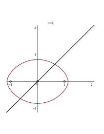
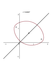
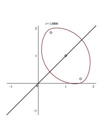
Figure 1. Parallel translation along the radial direction (from left to right)

In case of the radial direction the focal set of the translated trifocal ellipse at the parameter $t$ is $-X(t)$, ${\bf 0}$,

$$X(t)=\cos\left(t^{2}\right)\frac{\partial}{\partial u^{1}}_{(t,t)}-\sin\left(t^{2}\right)\frac{\partial}{\partial u^{2}}_{(t,t)}.$$

Figure 2 shows the parallel translates of the indicatrix along the circle $c(t)=(\cos(t),\sin(t)+1)$. The focal set of the translated trifocal ellipse at the parameter $t$ is $-X(t)$, ${\bf 0}$,

$$X(t)=\cos\left(1+\sin(t)\right)\frac{\partial}{\partial u^{1}}_{(\cos(t),1+\sin(t))}-\sin\left(1+\sin(t)\right)\frac{\partial}{\partial u^{2}}_{(\cos(t),1+\sin(t))}.$$

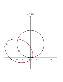
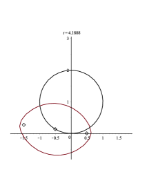
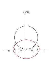
Figure 2. Parallel translation along the circle (from left to right)

The induced generalized Berwald plane is not conformally flat. To present examples for conformally flat generalized Berwald manifold it is sufficient and necessary to choose a closed (and, consequently, exact) $1$-form $\rho$.

References

- [1] I. Agricola and T. Friedrich, On the holonomy of connections with skew-symmetric torsion, Math. Ann. 328 (4) (2004), pp. 711-748.
- [2] D. Bao, On two curvature-driven problems in Riemann-Finsler geometry, Advanced Studies in Pure Mathematics 48, 2007, pp. 19-71.
- [3] D. Bao, S. - S. Chern and Z. Shen, An Introduction to Riemann-Finsler geometry, Springer-Verlag, 2000.
- [4] L. Berwald, Über zweidimensionale allgemeine metrische Räume, J. reine angew. Math. 156 (1927), 191-210 and 211-222.
- [5] L. Berwald, On Finsler and Cartan Geometries III, Two-dimensional Finsler spaces with rectilinear extremals, Ann. of Math. 42 (1941), 84-112.
- [6] M. Hashiguchi, On conformal transformations of Finsler metrics, J. Math. Kyoto Univ. 16 (1976), 25-50.
- [7] M. Hashiguchi and Y. Ichijy, On conformal transformations of Wagner spaces, Rep. Fac. Sci. Kagoshima Univ. (Math., Phys., Chem.) No. 10 (1977), 19-25.
- [8] M. Matsumoto, Foundations of Finsler Geometry and Special Finsler spaces, Kaisheisa Press, Otsu (1986).
- [9] M. Matsumoto, Conformally Berwald and conformally flat Finsler spaces, Publ. Math. Debrecen, 58 (1-2) (2001), 275-285.
- [10] Z. I. Szabó, Positive definite Berwald spaces. Structure theorems on Berwald spaces, Tensor (N. S.) 35 (1) (1981), pp. 25-39.
- [11] Sz. Vattamány and Cs. Vincze, On a new geometrical derivation of two-dimensional Finsler manifolds with constant main scalar, Period. Math. Hungar. 48 (1-2) (2004), 61-67.
- [12] Sz. Vattamány and Cs. Vincze, Two-dimensional Landsberg manifolds with vanishing Douglas tensor, Annales Univ. Sci. Budapest., 44 (2001), 11-26.
- [13] Cs. Vincze, An intrinsic version of Hashiguchi-Ichijyo’s theorems for Wagner manifolds, SUT J. Math. 35 (2) (1999), 263-270.
- [14] Cs. Vincze, On Wagner connections and Wagner manifolds, Acta Math. Hung. 89 (1-2) (2000), 111-133.
- [15] Cs. Vincze, A new proof of Szabó’s theorem on the Riemann-metrizability of Berwald manifolds, J. AMAPN, 21 (2005), 199-204.
- [16] Cs. Vincze, On a scale function for testing the conformality of Finsler manifolds to a Berwald manifold, Journal of Geometry and Physics. 54 (2005), 454-475.
- [17] Cs. Vincze, On geometric vector fields of Minkowski spaces and their applications, J. Diff. Geom. and Its Appl. 24 (2006), 1-20.
- [18] Cs. Vincze, On Berwald and Wagner manifolds, J. AMAPN, 24 (2008) 169-178.
- [19] Cs. Vincze, Generalized Berwald manifolds with semi-symmetric linear connections, Publ. Math. Debrecen 83 (4) (2013), pp. 741-755.
- [20] Cs. Vincze, On a special type of generalized Berwald manifolds: semi-symmetric linear connections preserving the Finslerian length of tangent vectors, European Journal of Mathematics, December 2017, Volume 3, Issue 4, pp 1098 - 1171.
- [21] Cs. Vincze, Lazy orbits: an optimization problem on the sphere, Journal of Geometry and Physics Volume 124, January 2018, Pages 180-198.
- [22] V. Wagner, On generalized Berwald spaces, CR Dokl. Acad. Sci. USSR (N.S.) 39 (1943), pp. 3-5.