Abstract

We study instancewise feature importance scoring as a method for model interpretation. Any such method yields, for each predicted instance, a vector of importance scores associated with the feature vector. Methods based on the Shapley score have been proposed as a fair way of computing feature attributions of this kind, but incur an exponential complexity in the number of features. This combinatorial explosion arises from the definition of the Shapley value and prevents these methods from being scalable to large data sets and complex models. We focus on settings in which the data have a graph structure, and the contribution of features to the target variable is well-approximated by a graph-structured factorization. In such settings, we develop two algorithms with linear complexity for instancewise feature importance scoring. We establish the relationship of our methods to the Shapley value and another closely related concept known as the Myerson value from cooperative game theory. We demonstrate on both language and image data that our algorithms compare favorably with other methods for model interpretation.

1 Introduction

Modern machine learning models, including random forests, deep neural networks, and kernel methods, can produce high-accuracy prediction in many applications. Often however, the accuracy in prediction from such black box models, comes at the cost of interpretability. Ease of interpretation is a crucial criterion when these tools are applied in areas such as medicine, financial markets, and criminal justice; for more background, see the discussion paper by Lipton [13] as well as references therein.

In this paper, we study instancewise feature importance scoring as a specific approach to the problem of interpreting the predictions of black-box models. Given a predictive model, such a method yields, for each instance to which the model is applied, a vector of importance scores associated with the underlying features. The instancewise property means that this vector, and hence the relative importance of each feature, is allowed to vary across instances. Thus, the importance scores can act as an explanation for the specific instance, indicating which features are the key for the model to make its prediction on that instance.

There is now a large body of research focused on the problem of scoring input features based on the prediction of a given instance (for instance, see the papers [19, 1, 17, 14, 22, 2, 5, 23] as well as references therein). Of most relevance to this paper is a line of recent work [22, 14, 5] that has developed methods for model interpretation based on Shapley value [18] from cooperative game theory. The Shapley value was originally proposed as an axiomatic characterization of a fair distribution of a total surplus from all the players, and can be applied in to predictive models, in which case each feature is modeled as a player in the underlying game. While the Shapley value approach is conceptually appealing, it is also computationally challenging: in general, each evaluation of a Shapley value requires an exponential number of model evaluations. Different approaches to circumventing this complexity barrier have been proposed, including those based on Monte Carlo approximation [22, 5] and methods based on sampled least-squares with weights [14].

In this paper, we take a complementary point of view, arguing that the problem of explanation is best approached within a model-based paradigm. In this view, explanations are cast in terms of a model, which may or may not be the same model as used to fit the data. Criteria such as Shapley value, which are intractable to compute when no assumptions are made, can be more effectively computed or approximated within the framework of a model. We focus specifically on settings in which a graph structure is appropriate for the data; specifically, we consider simple chains and grids, appropriate for time series and images, respectively. We propose two measures for instancewise feature importance scoring in this framework, which we term L-Shapley and C-Shapley; here the abbreviations “L" and “C" refer to “local” and “connected,” respectively. By exploiting the underlying graph structure, the number of model evaluations is reduced to linear—as opposed to exponential—in the number of features. We demonstrate the relationship of these measures with a constrained form of Shapley value, and we additionally relate C-Shapley with another solution concept from cooperative game theory, known as the Myerson value [16]. The Myerson value is commonly used in graph-restricted games, under a local additivity assumption of the model on disconnected subsets of features. Finally, we apply our feature scoring methods to several state-of-the-art models for both language and image data, and find that our scoring algorithms compare favorably to several existing sampling-based algorithms for instancewise feature importance scoring.

The remainder of this paper is organized as follows. We begin in Section 2 with background and set-up for the problem to be studied. In Section 3, we describe the two methods proposed and analyzed in this paper, based on the L-Shapley and C-Shapley scores. Section 4 is devoted to a study of the relationship between these scores and the Myerson value. In Section 5, we evaluate the performance of L-Shapley and C-Shapley on various real-world data sets, and we conclude with a discussion in Section 6.

2 Background and preliminaries

We begin by introducing some background and notation.

2.1 Importance of a feature subset

We are interested in studying models that are trained to perform prediction, taking as input a feature vector $x\in\mathcal{X}\subset^{d}$ and predicting a response or output variable $y\in\mathcal{Y}$. We assume access to the output of a model via a conditional distribution, denoted by $\mathbb{P}_{m}(\cdot|x)$, that provides the distribution of the response $Y\in\mathcal{Y}$ conditioned on a given vector $X=x$ of inputs. For any given subset $S\subset\{1,2,\ldots,d\}$, we use $x_{S}=\{x_{j},j\in S\}$ to denote the associated sub-vector of features, and we let $\mathbb{P}_{m}(Y\mid x_{S})$ denote the induced conditional distribution when $\mathbb{P}_{m}$ is restricted to using only the sub-vector $x_{S}$. In the cornercase in which $S=\emptyset$, we define $\mathbb{P}_{m}(Y\mid x_{\emptyset}):\,=\mathbb{P}_{m}(Y)$. In terms of this notation, for a given feature vector $x\in\mathcal{X}$, subset $S$ and fitted model distribution $\mathbb{P}_{m}(Y\mid x)$, we introduce the importance score

$$v_{x}(S):\,=\mathbb{E}_{m}\left[-\log\frac{1}{\mathbb{P}_{m}(Y\mid x_{S})}\;\Big{|}\;x\right],$$

where $\mathbb{E}_{m}[\cdot\mid x]$ denotes the expectation over $\mathbb{P}_{m}(\cdot\mid x)$. The importance score $v_{x}(S)$ has a coding-theoretic interpretation: it corresponds to the negative of the expected number of bits required to encode the output of the model based on the sub-vector $x_{S}$. It will be zero when the model makes a deterministic prediction based on $x_{S}$, and larger when the model returns a distribution closer to uniform over the output space.

There is also an information-theoretic interpretation to this definition of importance scores, as discussed in our previous work [3]. In particular, suppose that for a given integer $k<d$, there is a function $x\mapsto S^{*}(x)$ such that, for all almost all $x$, the $k$-sized subset $S^{*}(x)$ maximizes $v_{x}(S)$ over all subsets of size $k$. In this case, we are guaranteed that the mutual information $I(X_{S^{*}(X)},Y)$ between $X_{S^{*}(X)}$ and $Y$ is maximized, over any conditional distribution that generates a subset of size $k$ given $X$. The converse is also true.

In many cases, class-specific importance is favored, where one is interested in seeing how important a feature subset $S$ is to the predicted class, instead of the prediction as a conditional distribution. In order to handle such cases, it is convenient to introduce the degenerate conditional distribution

$$\hat{\mathbb{P}}_{m}(y\mid x) :\,=\begin{cases}1\text{ if }y\in\arg\max\limits_{y^{\prime}}\mathbb{P}_{m}(y^{\prime}\mid x),\\ 0\text{ otherwise.}\end{cases}$$

We can then define the importance of a subset $S$ with respect to $\hat{\mathbb{P}}_{m}$ using the modified score

$$v_{x}(S) :\,=\hat{\mathbb{E}}_{m}\left[-\log\frac{1}{\mathbb{P}_{m}(Y\mid x_{S})}\;\Big{|}\;x\right],$$

which is the expected log probability of the predicted class given the features in $S$.

Estimating the conditional distribution:

In practice, we need to estimate—for any given feature vector $\bar{x}\in\mathcal{X}$—the conditional probability functions $\mathbb{P}_{m}(y\mid\bar{x}_{S})$ based on observed data. Past work has used one of two approaches: either estimation based on empirical averages [22], or plug-in estimation using a reference point [5, 14].

Empirical average estimation: In this approach, we first draw a set of feature vector $\{x^{j}\}_{j=1}^{M}$ by sampling with replacement from the full data set. For each sample $x^{j}$, we define a new vector $\tilde{x}^{j}\in^{d}$ with components

$$(\tilde{x}_{j})_{i} =\begin{cases}\bar{x}_{i}&\mbox{if $i\in S$, and}\\ x^{j}_{i}&\mbox{otherwise.}\end{cases}$$

Taking the empirical mean of $\mathbb{P}_{m}(y\mid\tilde{x}^{j})$ over $\{\tilde{x}^{j}\}$ is then used as an estimate of $\mathbb{P}_{m}(y\mid\bar{x}_{S})$.

Plug-in estimation: In this approach, the first step is to specify a reference vector $x^{0}\in^{d}$ is specified. We then define the vector $\tilde{x}\in^{d}$ with components

$$(\tilde{x})_{i} =\begin{cases}\bar{x}_{i}&\mbox{if $i\in S$, and}\\ x^{0}_{i}&\mbox{otherwise}.\end{cases}$$

Finally, we use the conditional probability $\mathbb{P}_{m}(y\mid\tilde{x})$ as an approximation to $\mathbb{P}_{m}(y\mid\bar{x}_{S})$. The plug-in estimate is more computationally efficient than the empirical average estimator, and works well when there exist appropriate choices of reference points. We use this method for our experiments, where we use the index of padding for language data, and the average pixel strength of an image for vision data.

2.2 Shapley value for measuring interaction between features

Consider the problem of quantifying the importance of a given feature index $i$ for feature vector $x$. A naive way of doing so would be by computing the importance score $v_{x}(\{i\})$ of feature $i$ on its own. However, doing so ignores interactions between features, which are likely to be very important in applications. As a simple example, suppose that we were interested in performing sentiment analysis on the following sentence:

It is not heartwarming or entertaining. It just sucks. ($$\star$$)

This sentence is contained in a movie review from the IMDB movie data set [15], and it is classified as negative sentiment by a machine learning model to be discussed in the sequel. Now suppose we wish to quantify the importance of feature “not” in prediction. The word “not” plays an important role in the overall sentence as being classified as negative, and thus should be attributed a significant weight. However, viewed in isolation, the word “not” has neither negative nor positive sentiment, so that one would expect that $v_{x}(\{\mbox{``\emph{not}''}\})\approx 0$.

Thus, it is essential to consider the interaction of a given feature $i$ with other features. For a given subset $S$ containing $i$, a natural way in which to assess how $i$ interacts with the other features in $S$ is by computing the difference between the importance of all features in $S$, with and without $i$. This difference is called the marginal contribution of $i$ to $S$, and given by

$$m_{x}(S,i):\,=v_{x}(S)-v_{x}(S\setminus\{i\}).$$ (1)

In order to obtain a simple scalar measure for feature $i$, we need to aggregate these marginal contributions over all subsets that contain $i$. The Shapley value [18] is one principled way of doing so. For each integer $k=1,\ldots,d$, we let $\mathcal{S}_{k}(i)$ denote the set of $k$-sized subsets that contain $i$. The Shapley value is obtained by averaging the marginal contributions, first over the set $\mathcal{S}_{k}(i)$ for a fixed $k$, and then over all possible choices of set size $k$:

$$\phi_{x}(\mathbb{P}_{m},i):\,=\underbrace{\frac{1}{d}\sum_{k=1}^{d}}_{\mbox{Average over $k$}}\underbrace{\frac{1}{\binom{d-1}{k-1}}\sum_{S\in\mathcal{S}_{k}(i)}}_{\mbox{Average of over $\mathcal{S}_{k}(i)$}}m_{x}(S,i).$$ (2)

Since the model $\mathbb{P}_{m}$ remains fixed throughout our analysis, we frequently omit the dependence of $\phi_{x}$ on $\mathbb{P}_{m}$, instead adopting the more compact notation $\phi_{x}(i)$.

The concept of Shapley value was first introduced in cooperative game theory [18], and it has been used in a line of recent work on instancewise feature importance ranking [22, 5, 14]. It can be justified on an axiomatic basis [18, 24] as being the unique function from a collection of $2^{d}$ numbers (one for each subset $S$) to a collection of $d$ numbers (one for each feature $i$) with the following properties:

Additivity:

The sum of the Shapley values $\sum_{i=1}^{d}\phi_{x}(i)$ is equal to the difference $v_{x}(\{1,\ldots,d\})-v_{x}(\emptyset)$.

Equal contributions:

If $v_{x}(S\cup\{i\})=v_{x}(S\cup\{j\})$ for all subsets $S$, then $\phi_{x}(i)=\phi_{x}(j)$.

Monotonicity:

Given two models $\mathbb{P}_{m}$ and $\mathbb{P}_{m}$, let $m_{x}$ and $m_{x}^{\prime}$ denote the associated marginal contribution functions, and let $\phi_{x}$ and $\phi_{x}^{\prime}$ denote the associated Shapley values. If $m_{x}(S,i)\geq m^{\prime}_{x}(S,i)$ for all subsets $S$, then we are guaranteed that $\phi_{x}(i)\geq\phi^{\prime}_{x}(i)$.

Note that all three of these axioms are reasonable in our feature selection context.

2.3 The challenge with computing Shapley values

The exact computation of the Shapley value $\phi_{x}(i)$ takes into account the interaction of feature $i$ with all $2^{d-1}$ subsets that contain $i$, thereby leading to computational difficulties. Various approximation methods have been developed with the goal of reducing complexity. For example, Štrumbelj and Kononenko [22] proposed to estimate the Shapley values via a Monte Carlo approximation built on an alternative permutation-based definition of the Shapley value. Lundberg and Lee [14] proposed to evaluate the model over randomly sampled subsets and use a weighted linear regression to approximate the Shapley values based on the collected model evaluations.

In practice, such sampling-based approximations may suffer from high variance when the number of samples to be collected per instance is limited. For large-scale predictive models, the number of features is often relatively large, meaning that the number of samples required to obtain stable estimates can be prohibitively large. The main contribution of this paper is to address this challenge in a model-based paradigm, where the contribution of features to the response variable respects the structure of an underlying graph. In this setting, we propose efficient algorithms and provide bounds on the quality of the resulting approximation. As we discuss in more detail later, our approach should be viewed as complementary to sampling-based or regresssion-based approximations of the Shapley value. In particular, these methods can be combined with the approach of this paper so as to speed up the computation of the L-Shapley and C-Shapley values that we propose.

3 Methods

In many applications, the features can be associated with the nodes of a graph, and we can define distances between pairs of features based on the graph structure. More concretely, for sequence data (such as language, music etc.), each feature vector $x$ can be associated with a line graph, whereas for image data, each $x$ is naturally associated with a grid graph. In this section, we propose modified forms of the Shapley values, referred to as L-Shapley and C-Shapley values, that can be computed more efficiently than the Shapley value. We also show that under certain probabilistic assumptions on the marginal distribution over the features, these quantities yield good approximations to the original Shapley values.

More precisely, given feature vectors $x\in^{d}$, we let $G=(V,E)$ denote a connected graph with nodes $V$ and edges $E\subset V\times V$, where each feature $i$ is associated with a a node $i\in V$, and edges represent interactions between features. The graph induces a distance function on $V\times V$, given by

$$d_{G}(\ell,m) =\mbox{number of edges in shortest path joining $\ell$ to $m$}.$$ (3)

In the line graph, this graph distance corresponds to the number of edges in the unique path joining them, whereas it corresponds to the Manhattan distance in the grid graph. For a given node $i\in V$, its $k$-neighborhood is the set

$$\mathcal{N}_{k}(i) :\,=\left\{j\in V\mid d_{G}(i,j)\leq k\right\}$$ (4)

of all nodes at graph distance at most $k$. See Figure 1 for an illustration for the two-dimensional grid graph.

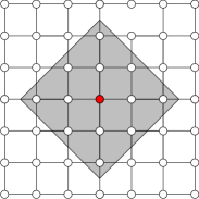
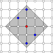
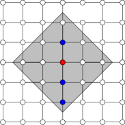
(a)		(b)		(c)

Figure 1: In all cases, the red node denotes the target feature $i$. (a) Illustration of the $k=2$ graph neighborhood $\mathcal{N}_{2}(i)$ on the grid graph. All nodes within the shaded gray triangle lie within the neighborhood $\mathcal{N}_{2}(i)$. (b) A disconnected subset of $\mathcal{N}_{2}(i)$ that is summed over in L-Shapley but not C-Shapley. (c) A connected subset of $\mathcal{N}_{2}(i)$ that is summed over in both L-Shapley and C-Shapley.

We propose two algorithms for the setting in which features that are either far apart on the graph or features that are not directly connected, have an accordingly weaker interaction.

3.1 Local Shapley

In order to motivate our first graph-structured Shapley score, let us take a deeper look at Example ($\star$ ‣ 2.2). In order to compute the importance score of “not,” the most important words to be included are “heartwarming” and “entertaining.” Intuitively, the words distant from them have a weaker influence on the importance of a given word in a document, and therefore have relatively less effect on the Shapley score. Accordingly, as one approximation, we propose the L-Shapley score, which only perturbs the neighboring features of a given feature when evaluating its importance:

Definition 1.

Given a model $\mathbb{P}_{m}$, a sample $x$ and a feature $i$, the L-Shapley estimate of order $k$ on a graph $G$ is given by

$$\hat{\phi}_{x}^{k}(i) :\,=\frac{1}{|\mathcal{N}_{k}(i)|}\sum_{\begin{subarray}{c}T\ni i\\ T\subseteq\mathcal{N}_{k}(i)\end{subarray}}\frac{1}{\binom{|\mathcal{N}_{k}(i)|-1}{|T|-1}}m_{x}(T,i).$$ (5)

The coefficients in front of the marginal contributions of feature $i$ are chosen to match the coefficients in the definition of the Shapley value restricted to the neighborhood $\mathcal{N}_{k}(i)$. We show in Section 4 that this choice controls the error under certain probabilistic assumptions. In practice, the choice of the integer $k$ is dictated by computational considerations. By the definition of $k$-neighborhoods, evaluating all $d$ L-Shapley scores on a line graph requires $2^{2k}d$ model evaluations. (In particular, computing each feature takes $2^{2k+1}$ model evaluations, half of which overlap with those of its preceding feature.) A similar calculation shows that computing all $d$ L-Shapley scores on a grid graph requires $2^{4k^{2}}d$ function evaluations.

3.2 Connected Shapley

We also propose a second algorithm, C-Shapley, that further reduces the complexity of approximating the Shapley value. Coming back to Example ($\star$ ‣ 2.2) where we evaluate the importance of “not,” both the L-Shapley estimate of order larger than two and the exact Shapley value estimate would evaluate the model on the word subset “It not heartwarming,” which rarely appears in real data and may not make sense to a human or a model trained on real-world data. The marginal contribution of “not” relative to “It not heartwarming” may be well approximated by the marginal contribution of “not” to “not heartwarming.” This motivates us to proprose C-Shapley:

Definition 2.

Given a model $\mathbb{P}_{m}$, a sample $x$ and a feature $i$, the C-Shapley estimate of order $k$ on a graph $G$ is given by

$$\tilde{\phi}_{x}^{k}(i) :\,=\sum_{U\in\mathcal{C}_{k}(i)}\frac{2}{(|U|+2)(|U|+1)|U|}m_{x}(U,i),$$ (6)

where $\mathcal{C}_{k}(i)$ denotes the set of all subsets of $\mathcal{N}_{k}(i)$ that contain node $i$, and are connected in the graph $G$.

The coefficients in front of the marginal contributions are a result of using Myerson value to characterize a new coalitional game over the graph $G$, in which the influence of disconnected subsets of features are additive. The error between C-Shapley and the Shapley value can also be controlled under certain statistical assumptions. See Section 4 for details.

For text data, C-Shapley is equivalent to only evaluating n-grams in a neighborhood of the word to be explained. By the definition of $k$-neighborhoods, evaluating the C-Shapley scores for all $d$ features takes $\mathcal{O}(k^{2}d)$ model evaluations on a line graph, as each feature takes $\mathcal{O}(k^{2})$ model evaluations.

4 Properties

In this section, we study some basic properties of the L-Shapley and C-Shapley values. In particular, under certain probabilistic assumptions on the features, we show that they provide good approximations to the original Shapley values. We also show their relationship to another concept from cooperative game theory, namely that of Myerson values, when the model satisfies certain local additivity assumptions.

4.1 Approximation of Shapley value

In order to characterize the relationship between L-Shapley and the Shapley value, we introduce absolute mutual information as a measure of dependence. Given two random variables $X$ and $Y$, the absolute mutual information $I_{a}(X;Y)$ between $X$ and $Y$ is defined as

$$I_{a}(X;Y)=\mathbb{E}\left[\Big{|}\log\frac{P(X,Y)}{P(X)P(Y)}\Big{|}\right],$$ (7)

where the expectation is taken jointly over $X,Y$. Based on the definition of independence, we have $I_{a}(X;Y)=0$ if and only if $X\mathchoice{\mathrel{\hbox to0.0pt{$\displaystyle\perp$\hss}\mkern 2.0mu{\displaystyle\perp}}}{\mathrel{\hbox to0.0pt{$\textstyle\perp$\hss}\mkern 2.0mu{\textstyle\perp}}}{\mathrel{\hbox to0.0pt{$\scriptstyle\perp$\hss}\mkern 2.0mu{\scriptstyle\perp}}}{\mathrel{\hbox to0.0pt{$\scriptscriptstyle\perp$\hss}\mkern 2.0mu{\scriptscriptstyle\perp}}}Y$. Recall the mutual information [4] is defined as $I(X;Y)=\mathbb{E}[\log\frac{P(X,Y)}{P(X)P(Y)}]$. The new measure is more stringent than the mutual information in the sense that $I(X;Y)\leq I_{a}(X;Y)$. The absolute conditional mutual information can be defined in an analogous way. Given three random variables $X,Y$ and $Z$, we define the absolute conditional mutual information to be $I_{a}(X;Y\mid Z)=\mathbb{E}[|\log\frac{P(X,Y\mid Z)}{P(X\mid Z)P(Y\mid Z)}|]$, where the expectation is taken jointly over $X,Y,Z$. Recall that $I_{a}(X;Y\mid Z)$ is zero if and only if $X\mathchoice{\mathrel{\hbox to0.0pt{$\displaystyle\perp$\hss}\mkern 2.0mu{\displaystyle\perp}}}{\mathrel{\hbox to0.0pt{$\textstyle\perp$\hss}\mkern 2.0mu{\textstyle\perp}}}{\mathrel{\hbox to0.0pt{$\scriptstyle\perp$\hss}\mkern 2.0mu{\scriptstyle\perp}}}{\mathrel{\hbox to0.0pt{$\scriptscriptstyle\perp$\hss}\mkern 2.0mu{\scriptscriptstyle\perp}}}Y|Z$.

Theorem 1 and Theorem 2 show that L-Shapley and C-Shapley values, respectively, are related to the Shapley value whenever the model obeys a Markovian structure that is encoded by the graph. We leave their proofs to Appendix B.

Theorem 1.

Suppose there exists a feature subset $S\subset\mathcal{N}_{k}(i)$ with $i\in S$, such that

$$\sup_{\begin{subarray}{c}U\subset S\setminus\{i\},V\subset[d]\setminus S\end{subarray}}I_{a}(X_{i};X_{V}|X_{U},Y)\leq\varepsilon;\sup_{\begin{subarray}{c}U\subset S\setminus\{i\},V\subset[d]\setminus S\end{subarray}}I_{a}(X_{i};X_{V}|X_{U})\leq\varepsilon,$$ (8)

where we identify $I_{a}(X_{i};X_{V}|X_{\emptyset})$ with $I_{a}(X_{i};X_{V})$ for notational convenience. Then the expected error between the L-Shapley estimate $\hat{\phi}_{X}^{k}(i)$ and the true Shapley-value-based importance score $\phi_{i}(\mathbb{P}_{m},x)$ is bounded by $4\varepsilon$:

$$\mathbb{E}_{X}|\hat{\phi}_{X}^{k}(i)-\phi_{X}(i)|\leq 4\varepsilon.$$ (9)

In particular, we have $\hat{\phi}_{X}^{k}(i)=\phi_{X}(i)$ almost surely if we have $X_{i}\mathchoice{\mathrel{\hbox to0.0pt{$\displaystyle\perp$\hss}\mkern 2.0mu{\displaystyle\perp}}}{\mathrel{\hbox to0.0pt{$\textstyle\perp$\hss}\mkern 2.0mu{\textstyle\perp}}}{\mathrel{\hbox to0.0pt{$\scriptstyle\perp$\hss}\mkern 2.0mu{\scriptstyle\perp}}}{\mathrel{\hbox to0.0pt{$\scriptscriptstyle\perp$\hss}\mkern 2.0mu{\scriptscriptstyle\perp}}}X_{[d]\setminus S}|X_{T}$ and $X_{i}\mathchoice{\mathrel{\hbox to0.0pt{$\displaystyle\perp$\hss}\mkern 2.0mu{\displaystyle\perp}}}{\mathrel{\hbox to0.0pt{$\textstyle\perp$\hss}\mkern 2.0mu{\textstyle\perp}}}{\mathrel{\hbox to0.0pt{$\scriptstyle\perp$\hss}\mkern 2.0mu{\scriptstyle\perp}}}{\mathrel{\hbox to0.0pt{$\scriptscriptstyle\perp$\hss}\mkern 2.0mu{\scriptscriptstyle\perp}}}X_{[d]\setminus S}|X_{T},Y$ for any $T\subset S\setminus\{i\}$.

Theorem 2.

Suppose there exists a neighborhood $S\subset\mathcal{N}_{k}(i)$ of $i$, with $i\in S$, such that Condition 8 is satisfied. Moreover, for any connected subset $U\subset S$ with $i\in U$, we have

$$\sup_{V\subset R(U)}I_{a}(X_{i};X_{V}|X_{U\setminus\{i\}},Y)\leq\varepsilon;\sup_{V\subset R(U)}I_{a}(X_{i};X_{V}|X_{U\setminus\{i\}})\leq\varepsilon,$$ (10)

where $R(U):\,=\{i\in[d]-U:\text{ for any }j\in U,(i,j)\notin E\}$. Then the expected error between the C-Shapley estimate $\tilde{\phi}_{X}^{k}(i)$ and the true Shapley-value-based importance score $\phi_{i}(\mathbb{P}_{m},x)$ is bounded by $6\varepsilon$:

$$\mathbb{E}_{X}|\tilde{\phi}_{X}^{k}(i)-\phi_{X}(i)|\leq 6\varepsilon.$$ (11)

In particular, we have $\hat{\phi}_{X}^{d}(i)=\phi_{X}(i)$ almost surely if we have $X_{i}\mathchoice{\mathrel{\hbox to0.0pt{$\displaystyle\perp$\hss}\mkern 2.0mu{\displaystyle\perp}}}{\mathrel{\hbox to0.0pt{$\textstyle\perp$\hss}\mkern 2.0mu{\textstyle\perp}}}{\mathrel{\hbox to0.0pt{$\scriptstyle\perp$\hss}\mkern 2.0mu{\scriptstyle\perp}}}{\mathrel{\hbox to0.0pt{$\scriptscriptstyle\perp$\hss}\mkern 2.0mu{\scriptscriptstyle\perp}}}X_{R(U)}|X_{U\setminus\{i\}}$ and $X_{i}\mathchoice{\mathrel{\hbox to0.0pt{$\displaystyle\perp$\hss}\mkern 2.0mu{\displaystyle\perp}}}{\mathrel{\hbox to0.0pt{$\textstyle\perp$\hss}\mkern 2.0mu{\textstyle\perp}}}{\mathrel{\hbox to0.0pt{$\scriptstyle\perp$\hss}\mkern 2.0mu{\scriptstyle\perp}}}{\mathrel{\hbox to0.0pt{$\scriptscriptstyle\perp$\hss}\mkern 2.0mu{\scriptscriptstyle\perp}}}X_{R(U)}|X_{U\setminus\{i\}},Y$ for any $U\subset[d]$.

4.2 Relating the C-Shapley value to the Myerson value

Let us now discuss how the C-Shapley value can be related to the Myerson value, which was introduced by Myerson [16] as an approach for characterizing a coalitional game over a graph $G$. Given a subset of nodes $S$ in the graph $G$, let $\mathcal{C}_{G}(S)$ denote the set of connected components of $S$—i.e., subsets of $S$ that are connected via edges of the graph. Thus, if $S$ is a connected subset of $G$, then $\mathcal{C}_{G}(S)$ consists only of $S$; otherwise, it contains a collection of subsets whose disjoint union is equal to $S$.

Consider a score function $T\mapsto v(T)$ that satisfies the following decomposability condition: for any subset of nodes $S$, the score $v(S)$ is equal to the sum of the scores over all the connected components of $S$—viz.

$$v(S) =\sum_{T\in\mathcal{C}_{G}(S)}v(T).$$ (12)

For any such score function, we can define the associated Shapley value, and it is known as the Myerson value on $G$ with respect to $v$. Myerson [16] showed that the Myerson value is the unique quantity that satisfies both the decomposability property, as well as the properties additivity, equal contributions and monotonicity given in Section 2.2.

In our setting, if we use a plug-in estimate for conditional probability, the decomposability condition (12) is equivalent to assuming that the influence of disconnected subsets of features are additive at sample $x$, and C-Shapley of order $k=d$ is exactly the Myerson value over $G$. In fact, if we partition each subset $S$ into connected components, as in the definition of Myerson value, and sum up the coefficients (using Lemma 1 in Appendix B), then the Myerson value is equivalent to equation (6).

4.3 Connections with related work

Let us now discuss connections with related work in more depth, and in particular how methods useful for approximating the Shapley value can be used to speed up the evaluation of approximate L-Shapley and C-Shapley values.

4.3.1 Sampling-based methods

There is an alternative definition of the Shapley value based on taking averages over permutations of the features. In particular, the contribution of a feature $i$ corresponds to the average of the marginal contribution of $i$ to its preceding features over the set of all permutations of $d$ features. Based on this definition, Štrumbelj and Kononenko [22] propose a Monte Carlo approximation, based on randomly sampling permutations.

While L-Shapley is deterministic in nature, it is possible to combine it with this and other sampling-based methods. For example, if one hopes to consider the interaction of features in a large neighborhood $\mathcal{N}_{k}(i)$ with a feature $i$, where exponential complexity in $k$ becomes a barrier, sampling based on random permutation of local features may be used to alleviate the computational burden.

4.3.2 Regression-based methods

Lundberg and Lee [14] proposed to sample feature subsets based on a weighted kernel, and carry out a weighted linear regression to estimate the Shapley value. Suppose the model is evaluated on $N$ feature subsets at $x$. In weighted least squares, each row of the data matrix $X\in\{0,1\}^{N\times d}$ is a $d$-dimensional vector, with the $j^{th}$ entry being one if the feature $j$ is selected, and zero otherwise. The response $F\in^{N}$ is the evaluation of the model over feature subsets. The weight matrix $W$ is diagonal with $W_{ii}=(d-1)/(\binom{d}{n_{i}}n_{i}(d-n_{i}))$ with $n_{i}=\sum_{j=1}^{d}X_{ij}$.

Lundberg and Lee [14] provide strong empirical results using this regression-based approximation, referred to as KernelSHAP; in particular, see Section 5.1 and Figure 3 of their paper. We can combine such a regression-based approximation with our modified Shapley values to further reduce the evaluation complexity of the C-Shapley values. In particular, for a chain graph, we evaluate the score function over all connected subsequences of length $\leq k$; similarly, on a grid graph, we evaluate it over all connected squares of size $\leq k\times k$. Doing so yields a data matrix $X\in\{0,1\}^{kd\times d}$ and a response vector $F\in^{kd}$, where $X_{ij}=1$ if the $j$th feature is included in the $i$th sample, and $F_{i}:\,=v_{x}(S_{i})$, the score function evaluated on the corresponding feature subset. We use the solution to this weighted least-squares problem as a regression-based estimate of C-Shapley—that is, $\tilde{\phi}^{k}_{x}\approx(X^{T}WX)^{-1}X^{T}F$.

5 Experiments

We evaluate the performance of L-Shapley and C-Shapley on real-world data sets involving text and image classification. Codes for reproducing the key results are available online. We compare L-Shapley and C-Shapley with several competitive algorithms for instancewise feature importance scoring on black-box models, including the regression-based approximation known as KernelSHAP [14], SampleShapley [22] , and the LIME method [17]. As discussed previously, KernelSHAP forms a weighted regression-approximation of the Shapley values, whereas SampleShapley estimates Shapley value by random permutation of features. The LIME method uses a linear model to locally approximate the original model through weighted least squares. For all methods, the number of model evaluations is the same, and linear in the number of features. We also choose the objective to be the log probability of the predicted class, and use the plug-in estimate of conditional probability across all methods (see Section 2.1).

For image data, we also compare with Saliency map [20] as another baseline. The Saliency method is used for interpreting neural networks in computer vision, by assuming knowledge of the gradient of a model with respect to the input, and using the gradient magnitude as the importance score for each pixel.

5.1 Text Classification

Text classification is a classical problem in natural language processing, in which text documents are assigned to predefined categories. We study the performance of L-Shapley and C-Shapley on three popular neural models for text classification: word-based CNNs [8], character-based CNNs [25], and long-short term memory (LSTM) recurrent neural networks [7], with the following three data sets on different scales. See Table 1 for a summary, and Appendix A for all of the details.

• IMDB Review with Word-CNN: The Internet Movie Review Dataset (IMDB) is a dataset of movie reviews for sentiment classification [15], which contains $50,000$ binary labeled movie reviews, with a split of $25,000$ for training and $25,000$ for testing. A simple word-based CNN model composed of an embedding layer, a convolutional layer, a max-pooling layer, and a dense layer is used, achieving an accuracy of $90.1\%$ on the test data set.

• AG news with Char-CNN: The AG news corpus is composed of titles and descriptions of $196,000$ news articles from $2,000$ news sources [25]. It is segmented into four classes, each containing $30,000$ training samples and $1,900$ testing samples. Our character-based CNN has the same structure as that proposed in Zhang et al. [25]. The model achieves an accuracy of $90.09\%$ on the test data set.

• Yahoo! Answers with LSTM: The corpus of Yahoo! Answers Topic Classification Dataset is divided into ten categories, each class containing $140,000$ training samples and $5,000$ testing samples. Each input text includes the question title, content and best answer. We train a bidirectional LSTM which achieves an accuracy of $70.84\%$ on the test data set, close to the state-of-the-art accuracy of $71.2\%$ obtained by character-based CNNs [25].

We choose zero paddings as the reference point for all methods, and make $4\times d$ model evaluations, where $d$ is the number of words for each input. Given the average length of each input (see Table 1), this choice controls the number of model evaluations under $1,000$, taking less than one second in TensorFlow on a Tesla K80 GPU for all the three models. For L-Shapley, we are able to consider the interaction of each word $i$ with the two neighboring words in $\mathcal{N}_{1}(i)$ given the budget. For C-Shapley, the budget allows the regression-based version to evaluate all $n$-grams with $n\leq 4$.

The change in log-odds scores before and after masking the top features ranked by importance scores is used as a metric for evaluating performance, where masked words are replaced by zero paddings. This metric has been used in previous literature in model interpretation [19, 14]. We study how the average log-odds score of the predicted class decreases as the percentage of masked features over the total number of features increases on $1,000$ samples from the test set. Results are plotted in Figure 2.

Data Set	Classes	Train Samples	Test Samples	Average #w	Model	Parameters	Accuracy
IMDB Review [15]	2	25,000	25,000	325.6	WordCNN	351,002	90.1%
AG’s News [25]	4	120,000	7,600	43.3	CharCNN	11,337,988	90.09%
Yahoo! Answers [25]	10	1,400,000	60,000	108.4	LSTM	7,146,166	70.84%

Table 1: A summary of data sets and models in three experiments. “Average #w” is the average number of words per sentence. “Accuracy” is the model accuracy on test samples.

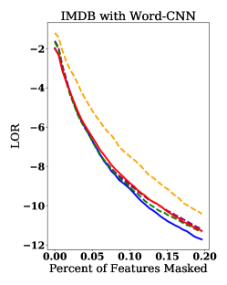
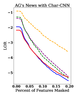
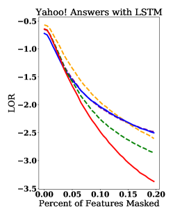
Figure 2: The above plots show the change in log odds ratio of the predicted class as a function of the percent of masked features, on the three text data sets. Lower log odds ratios are better.

Method	Explanation
Shapley	It is not heartwarming or entertaining. It just sucks.
C-Shapley	It is not heartwarming or entertaining. It just sucks.
L-Shapley	It is not heartwarming or entertaining. It just sucks.
KernelSHAP	It is not heartwarming or entertaining. It just sucks.
SampleShapley	It is not heartwarming or entertaining. It just sucks.

Table 2: Each word is highlighted with the RGB color as a linear function of its importance score. The background colors of words with positive and negative scores are linearly interpolated between blue and white, red and white respectively.

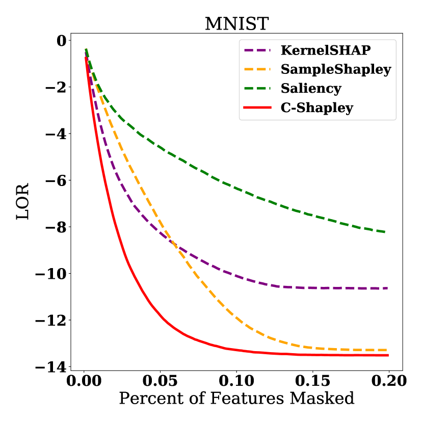
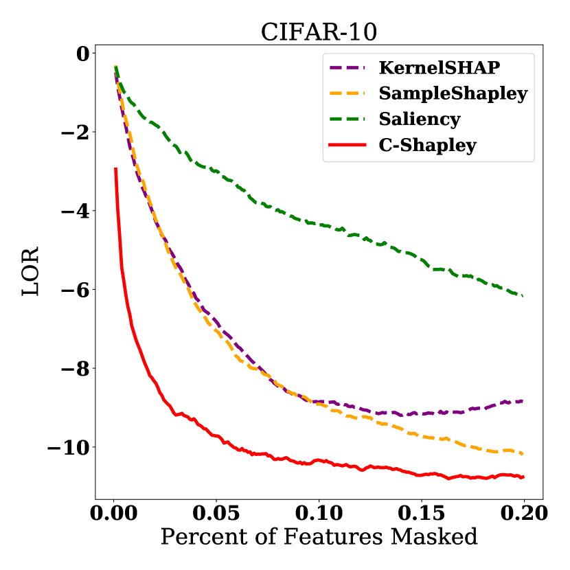
Figure 3: Left and Middle: change in log-odds ratio vs. the percent of pixels masked on MNIST and CIFAR10. Right: top pixels ranked by C-Shapley for a “$3$” and an “$8$” misclassified into “$8$” and “$3$” respectively. The masked pixels are colored with red if activated (white) and blue otherwise.

On IMDB with Word-CNN, the simplest model among the three, L-Shapley, achieves the best performance while LIME, KernelSHAP and C-Shapley achieve slightly worse performance. On AG’s news with Char-CNN, L-Shapley and C-Shapley both outperform other algorithms. On Yahoo! Answers with LSTM, C-Shapley outperforms the rest of the algorithms by a large margin, followed by LIME. L-Shapley with order $1$, SampleShapley, and KernelSHAP do not perform well for LSTM model, probably because some of the signals captured by LSTM are relatively long $n$-grams.

We also visualize the importance scores produced by different Shapley-based methods on Example ($\star$ ‣ 2.2), which is part of a negative movie review taken from IMDB. The result is shown in Table 2. More visualizations by our methods are available online.

5.2 Image Classification

We carry out experiments in image classification on the MNIST and CIFAR10 data sets:

• MNIST: The MNIST data set contains $28\times 28$ images of handwritten digits with ten categories $0-9$ [12]. A subset of MNIST data set composed of digits $3$ and $8$ is used for better visualization, with $12,000$ images for training and $1,000$ images for testing. A simple CNN model achieves $99.7\%$ accuracy on the test data set.

• CIFAR10: The CIFAR10 data set [10] contains $32\times 32$ images in ten classes. A subset of CIFAR10 data set composed of deers and horses is used for better visualization, with $10,000$ images for training and $2,000$ images for testing. A convolutional neural network modified from AlexNet [11] achieves $96.1\%$ accuracy on the test data set.

We take each pixel as a single feature for both MNIST and CIFAR10. We choose the average pixel strength as the reference point for all methods, and make $4\times d$ model evaluations, where $d$ is the number of pixels for each input image, which keeps the number of model evaluations under $4,000$.

LIME and L-Shapley are not used for comparison because LIME takes “superpixels” instead of raw pixels segmented by segmentation algorithms as single features, and L-Shapley requires nearly sixteen thousand model evaluations when applied to raw pixels. For C-Shapley, the budget allows the regression-based version to evaluate all $n\times n$ image patches with $n\leq 4$.

Figure 3 shows the decrease in log-odds scores before and after masking the top pixels ranked by importance scores as the percentage of masked pixels over the total number of pixels increases on $1,000$ test samples on MNIST and CIFAR10 data sets. C-Shapley consistently outperforms other methods on both data sets.

Figure 4 and Figure 5 provide additional visualization of the results. By masking the top pixels ranked by various methods, we find that the pixels picked by C-Shapley concentrate around and inside the digits in MNIST. The C-Shapley and Saliency methods yield the most interpretable results in CIFAR10. In particular, C-Shapley tends to mask the parts of head and body that distinguish deers and horses, and the human riding the horse. Figure 3 shows two misclassified digits by the CNN model. Interestingly, the top pixels chosen by C-Shapley visualize the “reasoning” of the model: more specifically, the important pixels to the model are exactly those which could form a digit from the opposite class.

Figure 4: Some examples of explanations obtained for the MNIST data set. The first row corresponds to the original images, with the rows below showing images masked based on scores produced by C-Shapley, KernelSHAP, SampleShapley and Saliency respectively. For best visualization results, 15% and 20% of the pixels are masked for each image. The masked pixels are colored with red if activated (white) and blue otherwise.

Figure 5: Some examples of explanations obtained for the CIFAR10 data set. The first row corresponds to the original images, with the rows below showing images masked based on scores produced by C-Shapley, KernelSHAP, SampleShapley and Saliency respectively. For best visualization results, 20% of the pixels are masked for each image.

6 Discussion

We have proposed L-Shapley and C-Shapley for instancewise feature importance scoring, making use of a graphical representation of the data. We have shown the superior performance of the proposed algorithms compared to other methods for instancewise feature importance scoring in text and image classification.

Appendix A Model structure

IMDB Review with Word-CNN

The word-based CNN model is composed of a $50$-dimensional word embedding, a $1$-D convolutional layer of 250 filters and kernel size three, a max-pooling and a $250$-dimensional dense layer as hidden layers. Both the convolutional and the dense layers are followed by ReLU as nonlinearity, and Dropout [21] as regularization. The model is trained with rmsprop [6]. The model achieves an accuracy of $90.1\%$ on the test data set.

AG’s news with Char-CNN

The character-based CNN has the same structure as the one proposed in Zhang et al. [25], composed of six convolutional layers, three max-pooling layers, and two dense layers. The model is trained with SGD with momentum 0.9 and decreasing step size initialized at $0.01$. (Details can be found in Zhang et al. [25].) The model reaches accuracy of $90.09\%$ on the test data set.

Yahoo! Answers with LSTM

The network consists of a $300$-dimensional randomly-initialized word embedding, a bidirectional LSTM, each LSTM unit of dimension $256$, and a dropout layer as hidden layers. The model is trained with rmsprop [6]. The model reaches accuracy of $70.84\%$ on the test data set, close to the state-of-the-art accuracy of $71.2\%$ obtained by character-based CNN [25].

MNIST

A simple CNN model is trained on the data set, which achieves $99.7\%$ accuracy on the test data set. It is composed of two convolutional layers of kernel size $5\times 5$ and a dense linear layer at last. The two convolutional layers contain 8 and 16 filters respectively, and both are followed by a max-pooling layer of pool size two.

CIFAR10

A convolutional neural network modified from AlexNet [11] is trained on the subset. It is composed of six convolutional layers of kernel size $3\times 3$ and two dense linear layers of dimension 512 and 256 at last. The six convolutional layers contain 48,48,96,96,192,192 filters respectively, and every two convolutional layers are followed by a max-pooling layer of pool size two and a dropout layer. The CNN model is trained with the Adam optimizer [9] and achieves $96.1\%$ accuracy on the test data set.

Appendix B Proof of Theorems

In this appendix, we collect the proofs of Theorems 1 and 2.

B.1 Proof of Theorem 1

We state an elementary combinatorial equality required for the proof of the main theorem:

Lemma 1 (A combinatorial equality).

For any positive integer $n$, and any pair of non-negative integers with $s\geq t$, we have

$$\sum_{j=0}^{n}\frac{1}{\binom{n+s}{j+t}}\binom{n}{j}=\frac{s+1+n}{(s+1)\binom{s}{t}}$$ (13)

Proof.

By the binomial theorem for negative integer exponents, we have

$$\frac{1}{(1-x)^{t+1}}=\sum_{j=0}^{\infty}\binom{j+t}{j}x^{j}.$$

The identity can be found by examination of the coefficient of $x^{n}$ in the expansion of

$$\frac{1}{(1-x)^{t+1}}\cdot\frac{1}{(1-x)^{s-t+1}}=\frac{1}{(1-x)^{s+1+1}}.$$ (14)

In fact, equating the coefficients of $x^{n}$ in the left and the right hand sides, we get

$$\sum_{j=0}^{n}\binom{j+t}{j}\binom{(n-j)+(s-t)}{n-j}=\binom{n+s+1}{n}=\frac{n+s+1}{s+1}\binom{n+s}{n}.$$ (15)

Moving $\binom{n+s}{n}$ to the right hand side and expanding the binomial coefficients, we have

$$\sum_{j=0}^{n}\frac{(j+t)!}{j!t!}\cdot\frac{(n-j+s-t)!}{(n-j)!(s-t)!}\cdot\frac{n!s!}{(n+s)!}=\frac{n+s+1}{s+1},$$ (16)

which implies

$$\sum_{j=0}^{n}\binom{n}{j}\binom{s}{t}\bigg{/}\binom{n+s}{j+t} =\sum_{j=0}^{n}\frac{n!}{(n-j)!j!}\cdot\frac{s!}{t!(s-t)!}\cdot\frac{((n+s)-(j+t))!(j+t)!}{(n+s)!}$$

$$=\sum_{j=0}^{n}\frac{(j+t)!}{j!t!}\cdot\frac{(n-j+s-t)!}{(n-j)!(s-t)!}\cdot\frac{n!s!}{(n+s)!}=\frac{n+s+1}{s+1}.$$

∎

Taking this lemma, we now prove the theorem. We split our analysis into two cases, namely $S=\mathcal{N}_{k}(i)$ versus $S\subset\mathcal{N}_{k}(i)$. For notational convenience, we extend the definition of L-Shapley estimate for feature $i$ to an arbitrary feature subset $S$ containing $i$. In particular, we define

$$\hat{\phi}_{x}^{S}(i) :\,=\frac{1}{|S|}\sum_{\begin{subarray}{c}T\ni i\\ T\subseteq S\end{subarray}}\frac{1}{\binom{|S|-1}{|T|-1}}m_{x}(T,i).$$ (17)

Case 1:

First, suppose that $S=\mathcal{N}_{k}(i)$. For any subset $A\subset[d]$, we introduce the shorthand notation $U_{S}(A):\,=A\cap S$ and $V_{S}(A):\,=A\cap S^{c}$, and note that $A=U_{S}(A)\cup V_{S}(A)$. Recalling the definition of the Shapley value, let us partition all the subsets $A$ based on $U_{S}(A)$, in particular writing

$$\phi_{X}(i) =\frac{1}{d}\sum_{\begin{subarray}{c}A\subseteq[d]\\ A\ni i\end{subarray}}\frac{1}{\binom{d-1}{|A|-1}}m_{X}(A,i)\;=\;\frac{1}{d}\sum_{\begin{subarray}{c}U\subseteq S\\ U\ni i\end{subarray}}\sum_{\begin{subarray}{c}A\subseteq[d]\\ U_{S}(A)=U\end{subarray}}\frac{1}{\binom{d-1}{|A|-1}}m_{X}(A,i).$$

Based on this partitioning, the expected error between $\hat{\phi}_{X}^{S}(i)$ and $\phi_{X}(i)$ can be written as

$$\mathbb{E}\left|\hat{\phi}_{X}^{S}(i)-\phi_{X}(i)\right| =\mathbb{E}\left|\frac{1}{|S|}\sum_{\begin{subarray}{c}U\subseteq S\\ U\ni i\end{subarray}}\frac{1}{\binom{|S|-1}{|U|-1}}m_{X}(U,i)-\frac{1}{d}\sum_{\begin{subarray}{c}U\subseteq S\\ U\ni i\end{subarray}}\sum_{\begin{subarray}{c}A\subseteq[d]\\ U_{S}(A)=U\end{subarray}}\frac{1}{\binom{d-1}{|A|-1}}m_{X}(A,i)\right|.$$ (18)

Partitioning the set $\{A:U_{S}(A)=U\}$ by the size of $V_{S}(A)=A\cap S^{c}$, we observe that

$$\sum_{\begin{subarray}{c}A\subseteq[d]\\ U_{S}(A)=U\end{subarray}}\frac{1}{\binom{d-1}{|A|-1}} =\sum_{i=0}^{d-|S|}\frac{1}{\binom{d-1}{i+|U|-1}}\binom{d-|S|}{i}$$

$$=\frac{(|S|-1)+1+(d-|S|)}{((|S|-1)+1)\binom{|S|-1}{|U|-1}}$$

$$=\frac{d}{|S|}\frac{1}{\binom{|S|-1}{|U|-1}},$$

where we have applied Lemma 1 with $n=d-|S|$, $s=|S|-1$, and $t=|U|-1$. Substituting this equivalence into equation (18), we find that the expected error can be upper bounded by

$$\mathbb{E}|\hat{\phi}_{X}^{S}(i)-\phi_{X}(i)| \leq\frac{1}{d}\sum_{\begin{subarray}{c}U\subseteq S\\ U\ni i\end{subarray}}\sum_{\begin{subarray}{c}A\subseteq[d]\\ U_{S}(A)=U\end{subarray}}\frac{1}{\binom{d-1}{|A|-1}}\mathbb{E}\left|m_{X}(U,i)-m_{X}(A,i)\right|,$$ (19)

where we recall that $A=U_{S}(A)\cup V_{S}(A)$.

Now omitting the dependence of $U_{S}(A),V_{S}(A)$ on $A$ for notational simplicity, we now write the difference as

$$m_{X}(A,i)-m_{X}(U,i) =\mathbb{E}_{m}\left[\log\frac{\mathbb{P}_{m}(Y|X_{U\cup V})}{\mathbb{P}_{m}(Y|X_{U\cup V\setminus\{i\}})}-\log\frac{\mathbb{P}_{m}(Y|X_{U})}{\mathbb{P}_{m}(Y|X_{U\setminus\{i\}})}\mid X\right]$$

$$=\mathbb{E}_{m}\left[\log\frac{\mathbb{P}(Y,X_{U\setminus\{i\}})\mathbb{P}(X_{U})P(X_{U\cup V\setminus\{i\}})P(X_{U\cup V},Y)}{\mathbb{P}(Y,X_{U})\mathbb{P}(X_{U\setminus\{i\}})P(X_{U\cup V})P(X_{U\cup V\setminus\{i\}},Y)}\mid X\right]$$

$$=\mathbb{E}_{m}\left[\log\frac{\mathbb{P}(X_{i},X_{V}\mid X_{U\setminus\{i\}},Y)}{\mathbb{P}(X_{i}\mid X_{U\setminus\{i\}},Y)\mathbb{P}(X_{V}\mid X_{U\setminus\{i\}},Y)}-\log\frac{\mathbb{P}(X_{i},X_{V}|X_{U\setminus\{i\}})}{\mathbb{P}(X_{i}|X_{U\setminus\{i\}})\mathbb{P}(X_{V}\mid X_{U\setminus\{i\}})}\mid X\right].$$

Substituting this equivalence into our earlier bound (19) and taking an expectation over $X$ on both sides, we find that the expected error is upper bounded as

$$\mathbb{E}|\hat{\phi}_{X}^{S}(i)-\phi_{X}(i)|\leq\frac{1}{d}\sum_{\begin{subarray}{c}U\subseteq S\\ U\ni i\end{subarray}}\sum_{\begin{subarray}{c}A\subseteq[d]\\ U_{S}(A)=U\end{subarray}}\frac{1}{\binom{d-1}{|A|-1}}\Biggr{\{}\mathbb{E}\left|\log\frac{\mathbb{P}(X_{i},X_{V_{S}(A)}|X_{U\setminus\{i\}},Y)}{\mathbb{P}(X_{i}|X_{U\setminus\{i\}},Y)\mathbb{P}(X_{V_{S}(A)}|X_{U\setminus\{i\}},Y)}\right|\\ +\mathbb{E}\left|\log\frac{\mathbb{P}(X_{i},X_{V_{S}(A)}|X_{U\setminus\{i\}})}{\mathbb{P}(X_{i}\mid X_{U\setminus\{i\}})\mathbb{P}(X_{V_{S}(A)}|X_{U\setminus\{i\}})}\right|\Biggr{\}}.$$

Recalling the definition of the absolute mutual information, we see that

$$\mathbb{E}|\hat{\phi}_{X}^{S}(i)-\phi_{X}(i)| \leq\frac{1}{d}\sum_{\begin{subarray}{c}U\subseteq S\\ U\ni i\end{subarray}}\sum_{\begin{subarray}{c}A\subseteq[d]\\ U_{S}(A)=U\end{subarray}}\frac{1}{\binom{d-1}{|A|-1}}\Big{\{}I_{a}(X_{i};X_{V_{S}(A)}\mid X_{U\setminus\{i\}},Y)+I_{a}(X_{i};X_{V_{S}(A)}\mid X_{U\setminus\{i\}})\Big{\}}$$

$$\leq 2\varepsilon,$$

which completes the proof of the claimed bound.

Finally, in the special case that $X_{i}\mathchoice{\mathrel{\hbox to0.0pt{$\displaystyle\perp$\hss}\mkern 2.0mu{\displaystyle\perp}}}{\mathrel{\hbox to0.0pt{$\textstyle\perp$\hss}\mkern 2.0mu{\textstyle\perp}}}{\mathrel{\hbox to0.0pt{$\scriptstyle\perp$\hss}\mkern 2.0mu{\scriptstyle\perp}}}{\mathrel{\hbox to0.0pt{$\scriptscriptstyle\perp$\hss}\mkern 2.0mu{\scriptscriptstyle\perp}}}X_{[d]\setminus S}|X_{T}$ and $X_{i}\mathchoice{\mathrel{\hbox to0.0pt{$\displaystyle\perp$\hss}\mkern 2.0mu{\displaystyle\perp}}}{\mathrel{\hbox to0.0pt{$\textstyle\perp$\hss}\mkern 2.0mu{\textstyle\perp}}}{\mathrel{\hbox to0.0pt{$\scriptstyle\perp$\hss}\mkern 2.0mu{\scriptstyle\perp}}}{\mathrel{\hbox to0.0pt{$\scriptscriptstyle\perp$\hss}\mkern 2.0mu{\scriptscriptstyle\perp}}}X_{[d]\setminus S}|X_{T},Y$ for any $T\subset S$, then this inequality holds with $\varepsilon=0$, which implies $\mathbb{E}|\hat{\phi}_{X}^{S}(i)-\phi_{X}(i)|=0$. Therefore, we have $\hat{\phi}_{X}^{S}(i)=\phi_{X}(i)$ almost surely, as claimed.

Case 2:

We now consider the general case in which $S\subset\mathcal{N}_{k}(i)$. Using the previous arguments, we can show

$$\mathbb{E}|\hat{\phi}_{X}^{S}(i)-\phi_{X}^{k}(i)|\leq 2\varepsilon,\quad\mbox{and}\quad\mathbb{E}|\hat{\phi}_{X}^{S}(i)-\phi_{X}(i)|\leq 2\varepsilon.$$

Appylying the triangle inequality yields $\mathbb{E}|\hat{\phi}_{X}^{k}(i)-\phi_{X}(i)|\leq 4\varepsilon$, which establishes the claim.

B.2 Proof of Theorem 2

As in the previous proof, we divide our analysis into two cases.

Case 1:

First, suppose that $S=\mathcal{N}_{k}(i)=[d]$. For any subset $A\subset S$ with $i\in A$, we can partition $A$ into two components $U_{S}(A)$ and $V_{S}(A)$, such that $i\in U_{S}(A)$ and $U_{S}(A)$ is a connected subsequence. $V_{S}(A)$ is disconnected from $U_{S}(A)$. We also define

$$\mathcal{C}=\{U\mid i\in U,U\subset[d],U\text{ is a connected subsequence.}\}$$ (20)

We partition all the subsets $A\subset S$ based on $U_{S}(A)$ in the definition of the Shapley value:

$$\phi_{X}(i) =\frac{1}{d}\sum_{\begin{subarray}{c}A\subseteq S\\ A\ni i\end{subarray}}\frac{1}{\binom{d-1}{|A|-1}}m_{X}(A,i)$$

$$=\frac{1}{d}\sum_{U\in\mathcal{C}}\sum_{A:U_{S}(A)=U}\frac{1}{\binom{d-1}{|A|-1}}m_{X}(A,i).$$

The expected error between $\tilde{\phi}_{X}^{[d]}(i)$ and $\phi_{X}(i)$ is

$$\mathbb{E}|\tilde{\phi}_{X}^{[d]}(i)-\phi_{X}(i)|=\mathbb{E}\left|\frac{1}{d}\sum_{U\in\mathcal{C}}\frac{2d}{(|U|+2)(|U|+1)|U|}m_{X}(U,i)-\frac{1}{d}\sum_{U\in\mathcal{C}}\sum_{A:U_{S}(A)=U}\frac{1}{\binom{d-1}{|A|-1}}m_{X}(A,i)\right|.$$ (21)

Partitioning $\{A:U_{S}(A)=U\}$ by the size of $V_{S}(A)$, we observe that

$$\sum_{A:U_{S}(A)=U}\frac{1}{\binom{d-1}{|A|-1}} =\sum_{i=0}^{d-|U|-2}\frac{1}{\binom{d-1}{i+|U|-1}}\binom{d-|U|-2}{i}$$

$$=\frac{(|U|+1)+1+(d-|U|-2)}{((|U|+1)+1)\binom{|U|+1}{|U|-1}}$$

$$=\frac{2d}{(|U|+2)(|U|+1)|U|},$$

where we apply Lemma 1 with $n=d-|U|-2$, $s=|U|+1$ and $t=|U|-1$. From equation (21), the expected error can be upper bounded by

$$\mathbb{E}\left|\tilde{\phi}_{X}^{[d]}(i)-\phi_{X}(i)\right| \leq\frac{1}{d}\sum_{U\in\mathcal{C}}\sum_{A:U_{S}(A)=U}\frac{1}{\binom{d-1}{|A|-1}}\mathbb{E}\left|m_{X}(U,i)-m_{X}(A,i)\right|,$$

where $A=U_{S}(A)\cup V_{S}(A)$. We omit the dependence of $U_{S}(A)$ and $V_{S}(A)$ on the pair $(A,S)$ for notational simplicity, and observe that the difference between $m_{x}(A,i)$ and $m_{x}(U,i)$ is

$$m_{X}(A,i)-m_{X}(U,i) =\mathbb{E}_{m}\left[\log\frac{\mathbb{P}_{m}(Y|X_{U\cup V})}{\mathbb{P}_{m}(Y|X_{U\cup V\setminus\{i\}})}-\log\frac{\mathbb{P}_{m}(Y|X_{U})}{\mathbb{P}_{m}(Y|X_{U\setminus\{i\}})}\mid X\right]$$

$$=\mathbb{E}_{m}\left[\log\frac{\mathbb{P}(Y,X_{U\setminus\{i\}})\mathbb{P}(X_{U})P(X_{U\cup V\setminus\{i\}})P(X_{U\cup V},Y)}{\mathbb{P}(Y,X_{U})\mathbb{P}(X_{U\setminus\{i\}})P(X_{U\cup V})P(X_{U\cup V\setminus\{i\}},Y)}\mid X\right]$$

$$=\mathbb{E}_{m}\left[\log\frac{\mathbb{P}(X_{i},X_{V}|X_{U\setminus\{i\}},Y)}{\mathbb{P}(X_{i}|X_{U\setminus\{i\}},Y)\mathbb{P}(X_{V}|X_{U\setminus\{i\}},Y)}-\log\frac{\mathbb{P}(X_{i},X_{V}|X_{U\setminus\{i\}})}{\mathbb{P}(X_{i}|X_{U\setminus\{i\}})\mathbb{P}(X_{V}|X_{U\setminus\{i\}})}\mid X\right].$$

Taking an expectation over $X$ at both sides, we can upper bound the expected error by

$$\mathbb{E}|\tilde{\phi}_{X}^{[d]}(i)-\phi_{X}(i)| \leq\frac{1}{d}\sum_{U\in\mathcal{C}}\sum_{A:U_{S}(A)=U}\frac{1}{\binom{d-1}{|A|-1}}(\mathbb{E}\left|\log\frac{\mathbb{P}(X_{i},X_{V_{S}(A)}|X_{U\setminus\{i\}},Y)}{\mathbb{P}(X_{i}|X_{U\setminus\{i\}},Y)\mathbb{P}(X_{V_{S}(A)}|X_{U\setminus\{i\}},Y)}\right|$$

$$\qquad\qquad\qquad\qquad\qquad\quad+\mathbb{E}\left|\log\frac{\mathbb{P}(X_{i},X_{V_{S}(A)}|X_{U\setminus\{i\}})}{\mathbb{P}(X_{i}|X_{U\setminus\{i\}})\mathbb{P}(X_{V_{S}(A)}|X_{U\setminus\{i\}})}\right|)$$

$$=\frac{1}{d}\sum_{U\in\mathcal{C}}\sum_{A:U_{S}(A)=U}\frac{1}{\binom{d-1}{|A|-1}}(I_{a}(X_{i};X_{V_{S}(A)}|X_{U\setminus\{i\}},Y)+I_{a}(X_{i};X_{V_{S}(A)}|X_{U\setminus\{i\}}))$$

$$\leq 2\varepsilon.$$

Let $R(U):\,=[d]-U\cup\{\max(u-1,1),\min(u+l+1,d)\}$. If we have $X_{i}\mathchoice{\mathrel{\hbox to0.0pt{$\displaystyle\perp$\hss}\mkern 2.0mu{\displaystyle\perp}}}{\mathrel{\hbox to0.0pt{$\textstyle\perp$\hss}\mkern 2.0mu{\textstyle\perp}}}{\mathrel{\hbox to0.0pt{$\scriptstyle\perp$\hss}\mkern 2.0mu{\scriptstyle\perp}}}{\mathrel{\hbox to0.0pt{$\scriptscriptstyle\perp$\hss}\mkern 2.0mu{\scriptscriptstyle\perp}}}X_{R(U)}|X_{U\setminus\{i\}}$ and $X_{i}\mathchoice{\mathrel{\hbox to0.0pt{$\displaystyle\perp$\hss}\mkern 2.0mu{\displaystyle\perp}}}{\mathrel{\hbox to0.0pt{$\textstyle\perp$\hss}\mkern 2.0mu{\textstyle\perp}}}{\mathrel{\hbox to0.0pt{$\scriptstyle\perp$\hss}\mkern 2.0mu{\scriptstyle\perp}}}{\mathrel{\hbox to0.0pt{$\scriptscriptstyle\perp$\hss}\mkern 2.0mu{\scriptscriptstyle\perp}}}X_{R(U)}|X_{U\setminus\{i\}},Y$ for any $U\subset[d]$, then $\varepsilon=0$, which implies $\mathbb{E}|\tilde{\phi}_{X}^{[d]}(i)-\phi_{X}(i)|=0$. Therefore, we have $\tilde{\phi}_{X}^{[d]}(i)=\phi_{X}(i)$ almost surely.

Case 2:

We now turn to the general case $S\subset\mathcal{N}_{k}(i)\subset[d]$. Similar as above, we can show

$$\mathbb{E}|\tilde{\phi}_{X}^{k}(i)-\hat{\phi}_{X}^{k}(i)|\leq 2\varepsilon.$$

Based on Theorem 1, we have

$$\mathbb{E}|\hat{\phi}_{X}^{k}(i)-\phi_{X}(i)| \leq 4\varepsilon.$$

Applying the triangle yields $\mathbb{E}|\tilde{\phi}_{X}^{k}(i)-\phi_{X}(i)|\leq 6\varepsilon$, which establishes the claim.

References

- Bach et al. [2015] Sebastian Bach, Alexander Binder, Grégoire Montavon, Frederick Klauschen, Klaus-Robert Müller, and Wojciech Samek. On pixel-wise explanations for non-linear classifier decisions by layer-wise relevance propagation. PloS One, 10(7):e0130140, 2015.
- Baehrens et al. [2010] David Baehrens, Timon Schroeter, Stefan Harmeling, Motoaki Kawanabe, Katja Hansen, and Klaus-Robert Müller. How to explain individual classification decisions. Journal of Machine Learning Research, 11:1803–1831, 2010.
- Chen et al. [2018] Jianbo Chen, Le Song, Martin J Wainwright, and Michael I Jordan. Learning to explain: An information-theoretic perspective on model interpretation. arXiv preprint arXiv:1802.07814, 2018.
- Cover and Thomas [2012] Thomas M Cover and Joy A Thomas. Elements of Information Theory. John Wiley & Sons, 2012.
- Datta et al. [2016] Anupam Datta, Shayak Sen, and Yair Zick. Algorithmic transparency via quantitative input influence: Theory and experiments with learning systems. In Security and Privacy (SP), 2016 IEEE Symposium on, pages 598–617. IEEE, 2016.
- [6] Geoffrey Hinton, Nitish Srivastava, and Kevin Swersky. Neural networks for machine learning-lecture 6a-overview of mini-batch gradient descent.
- Hochreiter and Schmidhuber [1997] Sepp Hochreiter and Jürgen Schmidhuber. Long short-term memory. Neural Computation, 9(8):1735–1780, 1997.
- Kim [2014] Yoon Kim. Convolutional neural networks for sentence classification. In Proceedings of the 2014 Conference on Empirical Methods in Natural Language Processing (EMNLP), pages 1746–1751, 2014.
- Kingma and Ba [2015] Diederik P Kingma and Jimmy Ba. Adam: A method for stochastic optimization. In Proceedings of the International Conference on Learning Representations (ICLR), 2015.
- Krizhevsky [2009] Alex Krizhevsky. Learning multiple layers of features from tiny images. 2009.
- Krizhevsky et al. [2012] Alex Krizhevsky, Ilya Sutskever, and Geoffrey E Hinton. Imagenet classification with deep convolutional neural networks. In Advances in Neural Information Processing Systems, pages 1097–1105, 2012.
- LeCun et al. [1998] Yann LeCun, Léon Bottou, Yoshua Bengio, and Patrick Haffner. Gradient-based learning applied to document recognition. Proceedings of the IEEE, 86(11):2278–2324, 1998.
- Lipton [2016] Zachary C Lipton. The mythos of model interpretability. arXiv preprint arXiv:1606.03490, 2016.
- Lundberg and Lee [2017] Scott M Lundberg and Su-In Lee. A unified approach to interpreting model predictions. In I. Guyon, U. V. Luxburg, S. Bengio, H. Wallach, R. Fergus, S. Vishwanathan, and R. Garnett, editors, Advances in Neural Information Processing Systems 30, pages 4765–4774. Curran Associates, Inc., 2017. URL http://papers.nips.cc/paper/7062-a-unified-approach-to-interpreting-model-predictions.pdf.
- Maas et al. [2011] Andrew L Maas, Raymond E Daly, Peter T Pham, Dan Huang, Andrew Y Ng, and Christopher Potts. Learning word vectors for sentiment analysis. In Proceedings of the 49th Annual Meeting of the Association for Computational Linguistics, pages 142–150. Association for Computational Linguistics, 2011.
- Myerson [1977] Roger B Myerson. Graphs and cooperation in games. Mathematics of Operations Research, 2(3):225–229, 1977.
- Ribeiro et al. [2016] Marco Tulio Ribeiro, Sameer Singh, and Carlos Guestrin. Why should I trust you?: Explaining the predictions of any classifier. In Proceedings of the 22nd ACM SIGKDD International Conference on Knowledge Discovery and Data Mining, pages 1135–1144. ACM, 2016.
- Shapley [1953] Lloyd S Shapley. A value for n-person games. Contributions to the Theory of Games, 2(28):307–317, 1953.
- Shrikumar et al. [2017] Avanti Shrikumar, Peyton Greenside, and Anshul Kundaje. Learning important features through propagating activation differences. In ICML, volume 70 of Proceedings of Machine Learning Research, pages 3145–3153. PMLR, 06–11 Aug 2017.
- Simonyan et al. [2014] K. Simonyan, A. Vedaldi, and A. Zisserman. Deep inside convolutional networks: Visualising image classification models and saliency maps. In Proceedings of the International Conference on Learning Representations (ICLR), 2014.
- Srivastava et al. [2014] Nitish Srivastava, Geoffrey Hinton, Alex Krizhevsky, Ilya Sutskever, and Ruslan Salakhutdinov. Dropout: A simple way to prevent neural networks from overfitting. The Journal of Machine Learning Research, 15(1):1929–1958, 2014.
- Štrumbelj and Kononenko [2010] Erik Štrumbelj and Igor Kononenko. An efficient explanation of individual classifications using game theory. Journal of Machine Learning Research, 11:1–18, 2010.
- Sundararajan et al. [2017] Mukund Sundararajan, Ankur Taly, and Qiqi Yan. Axiomatic attribution for deep networks. In International Conference on Machine Learning, pages 3319–3328, 2017.
- Young [1985] H Peyton Young. Monotonic solutions of cooperative games. International Journal of Game Theory, 14(2):65–72, 1985.
- Zhang et al. [2015] Xiang Zhang, Junbo Zhao, and Yann LeCun. Character-level convolutional networks for text classification. In Advances in Neural Information Processing Systems, pages 649–657, 2015.