Short distance asymptotics for a generalized two-point scaling function in the two-dimensional Ising model

Abstract.

In the 1977 paper [21] of B. McCoy, C. Tracy and T. Wu it was shown that the limiting two-point correlation function in the two-dimensional Ising model is related to a second order nonlinear Painlevé function. This result identified the scaling function as a tau-function and the corresponding connection problem was solved by C. Tracy in 1991 [27], see also the works by C. Tracy and H. Widom in 1998 [28]. Here we present the solution to a certain generalized version of the above connection problem which is obtained through a refinement of the techniques chosen in [3].

1. Introduction and statement of results

This note is concerned with the solution of a generalized connection problem for a distinguished tau-function of the $\nu$-modified radial sinh-Gordon equation.

1.1. Modified sinh-Gordon equation and connection problem

In 1977, B. McCoy, C. Tracy and T. Wu derived the following result.

Theorem 1.1 (McCoy, Tracy, Wu [21], 1977).

Let

$$f_{2n}(t;\nu):=\frac{(-1)^{n}}{n}\int_{1}^{\infty}\cdots\int_{1}^{\infty}\left[\prod_{j=1}^{2n}\frac{\mathrm{e}^{-ty_{j}}}{\sqrt{y_{j}^{2}-1}}\left(\frac{y_{j}-1}{y_{j}+1}\right)^{\nu}\frac{1}{y_{j}+y_{j+1}}\right]\prod_{j=1}^{n}\big{(}y_{2j}^{2}-1\big{)}\prod_{j=1}^{2n}{\mathrm{d}}y_{j},\ \ n\in\mathbb{Z}_{\geq 1},$$

with $y_{2n+1}\equiv y_{1},t>0$ and $\nu>-\frac{1}{2}$. Then for any $\lambda\in[0,\frac{1}{\pi}]$,

$$\exp\left[-\sum_{n=1}^{\infty}\lambda^{2n}f_{2n}(t;\nu)\right]=\exp\bigg{\{}\frac{1}{4}\int_{t}^{\infty}\left[\sinh^{2}\psi-\left(\frac{{\mathrm{d}}\psi}{{\mathrm{d}}s}\right)^{2}+\frac{4\nu}{s}\sinh^{2}\left(\frac{\psi}{2}\right)\right]s\,{\mathrm{d}}s\bigg{\}}\cosh\left(\frac{\psi}{2}\right),$$ (1.1)

where $\psi=\psi(t;\nu,\lambda)\in\mathbb{R}$ solves the second order nonlinear ODE

$$\frac{{\mathrm{d}}^{2}\psi}{{\mathrm{d}}t^{2}}+\frac{1}{t}\frac{{\mathrm{d}}\psi}{{\mathrm{d}}t}=\frac{1}{2}\sinh(2\psi)+\frac{2\nu}{t}\sinh\psi,$$ (1.2)

subject to the boundary condition

$$\psi(t;\nu,\lambda)\sim 2\lambda\int_{1}^{\infty}\frac{\mathrm{e}^{-ty}}{\sqrt{y^{2}-1}}\left(\frac{y-1}{y+1}\right)^{\nu}\,{\mathrm{d}}y\ \ \ \ \textnormal{as}\ \ t\rightarrow+\infty.$$ (1.3)

The right-hand side in (1.1), which we shall abbreviate as $\tau(t;\nu,\lambda)$ below, appeared first in the Wu, McCoy, Tracy, Barouch analysis [31] of the scaling limit of the spin-spin correlation function in the 2D Ising model. In a nutshell (cf. [22, 24] for more details), if $\xi=\xi(T)$ is the temperature dependent correlation length (which diverges as $|T-T_{c}|^{-1}$ near the critical temperature $T_{c}$) and $\langle\sigma_{00}\sigma_{MN}\rangle$ the 2-point function on an isotropic Onsager lattice after the thermodynamic limit, then

$$R^{\frac{1}{4}}\langle\sigma_{00}\sigma_{MN}\rangle\rightarrow F_{\pm}(t),$$ (1.4)

holds true in the massive scaling limit $\xi\rightarrow\infty,R=\sqrt{M^{2}+N^{2}}\rightarrow\infty$ such that $t=R/\xi>0$ is fixed. The $\pm$ choice refers to the scaling limit taken either above or below the critical temperature $T_{c}$ and $F_{\pm}(t)$ are the so-called scaling functions given by

$$F_{-}(t)=2^{\frac{3}{8}}t^{\frac{1}{4}}\tau\left(t,0,\frac{1}{\pi}\right)\ \ \ \ \ \ \ \ \textnormal{and}\ \ \ \ \ \ \ \ F_{+}(t)=F_{-}(t)\tanh\left[\frac{1}{2}\psi\left(t;0,\frac{1}{\pi}\right)\right].$$ (1.5)

The nonlinear equation (1.2), coined $\nu$-modified radial sinh-Gordon equation, is intimately related to Painlevé special function theory since $u(t;\nu,\lambda):=\mathrm{e}^{-\psi(2t;\nu,\lambda)}$ solves

$$\frac{{\mathrm{d}}^{2}u}{{\mathrm{d}}t^{2}}=\frac{1}{u}\left(\frac{{\mathrm{d}}u}{{\mathrm{d}}t}\right)^{2}-\frac{1}{t}\frac{{\mathrm{d}}u}{{\mathrm{d}}t}+\frac{2\nu}{t}\big{(}u^{2}-1\big{)}+u^{3}-\frac{1}{u},$$ (1.6)

which, cf. [23, $32.2.3$], is Painlevé-III with constants $(\alpha,\beta,\gamma,\delta)=(2\nu,-2\nu,1,-1)$. Historically, (1.2), resp. (1.6), was the very first appearance of a Painlevé function in a problem of mathematical physics - predating various field theoretic or nonlinear wave theoretic applications and in particular predating their numerous appearances in quantum gravity, enumerative toplogy, random matrix theory, combinatorics, integrable probability, etc. It is known that $\psi(t;\nu,\lambda)$, uniquely determined by the above specified $+\infty$ behavior, is a highly transcendental function which cannot be expressed in terms of known classical special functions (i.e. not in terms of a finite number of contour integrals of elementary, or elliptic or finite genus algebraic functions). This fact turns the underlying connection problem, i.e. the problem of computing the $t\downarrow 0$ behavior of $\psi(t;\nu,\lambda)$ from its known $t\rightarrow+\infty$ asymptotics (or vice versa), into a challenging and foremost nonstandard task. Nowadays powerful analytical techniques of inverse scattering, isomonodromy or Riemann-Hilbert theory allow us to derive the underlying connection formulæ  in a systematic fashion. Again, [21] predates these approaches and McCoy, Tracy and Wu had, for the very first time, derived a complete connection formula in case of (1.2), resp. (1.6). In detail, they showed in [21, $1.10$] that for fixed $\lambda\in[0,\frac{1}{\pi})$ the small $t$-expansion of $u(t;\nu,\lambda)$ is given by

$$u\Big{(}\frac{t}{2};\nu,\lambda\Big{)}=Bt^{\sigma}\left(1-\frac{\nu}{B}(1-\sigma)^{-2}t^{1-\sigma}+B\nu(1+\sigma)^{-2}t^{1+\sigma}+\mathcal{O}\big{(}t^{2(1-\sigma)}\big{)}\right),$$ (1.7)

with $(t,\nu,\lambda)$-differentiable error terms and where $(\sigma,B)$ are the following functions of $(\nu,\lambda)$,

$$\sigma=\frac{2}{\pi}\arcsin(\pi\lambda)\in[0,1);\ \ \ \ B=2^{-3\sigma}\frac{\Gamma^{2}(\frac{1}{2}(1-\sigma))}{\Gamma^{2}(\frac{1}{2}(1+\sigma))}\frac{\Gamma(\nu+\frac{1}{2}(1+\sigma))}{\Gamma(\nu+\frac{1}{2}(1-\sigma))},$$ (1.8)

in terms of Euler’s Gamma function $\Gamma(z)$, cf. [23, $5.2.1$]. Note that $B=B(\nu,\sigma)$ might vanish for $\nu<0$, thus expansion (1.7) holds uniformly in $(\sigma,\nu)\in[0,1)\times(-\frac{1}{2},+\infty)\setminus\{\sigma=1+2\nu\}$ chosen from compact subsets. Also, $B=B(\nu,\sigma)$ is negative iff $\sigma>1+2\nu$, compare Figure 1 below. Hence, given our connection of $u(t;\nu,\lambda)=\mathrm{e}^{-\psi(2t;\nu,\lambda)}\geq 0$ to the real-valued scaling functions in the 2D Ising model (1.1), we shall in the following restrict ourselves, whenever working with (1.7) and (1.8), to the values $(\sigma,\nu)\in[0,1)\times(-\frac{1}{2},+\infty)$ for which $\sigma<1+2\nu$.

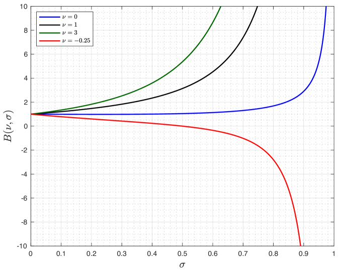
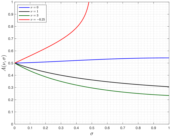
Figure 1. The coefficient $B=B(\nu,\sigma)$ as function of $\sigma\in[0,1]$ for varying $\nu>-\frac{1}{2}$ on the left. On the right we display $A=A(\nu,\sigma)$ as computed in Theorem 1.2 below for $\sigma\in[0,1]$ with varying $\nu>-\frac{1}{2}$ such that $\nu+\frac{1}{2}(1-\sigma)>0$.

In addition to (1.7), [21, $4.119$] also investigated the behavior of $u(t;\nu,\lambda)$ in the limit $\sigma\uparrow 1$ ($\lambda\uparrow\frac{1}{\pi}$) for small enough $t$ and obtained

$$u\Big{(}\frac{t}{2};\nu,\frac{1}{\pi}\Big{)}=\frac{t}{2}\left\{\nu\ln^{2}t-c(\nu)\ln t+\frac{1}{4\nu}\big{(}c^{2}(\nu)-1\big{)}\right\}+o(1),$$ (1.9)

where $c(\nu)=1+2\nu\big{(}3\ln 2-2\gamma_{E}-\psi_{0}(1+\nu)\big{)}$ which is defined in terms of the digamma function $\psi_{0}(z)$, cf. [23, $5.2.2$], and Euler’s constant $\gamma_{E}$, cf. [23, $5.2.3$].

1.2. Hamiltonian structure

Equation (1.2) is expressible as the Hamiltonian system

$$\frac{{\mathrm{d}}q}{{\mathrm{d}}t}=\frac{\partial H}{\partial p},\ \ \ \frac{{\mathrm{d}}p}{{\mathrm{d}}t}=-\frac{\partial H}{\partial q},\ \ \ \ \ \ \ H=H(q,p,t,\nu)=\frac{t}{2}\sinh^{2}q-\frac{p^{2}}{2t}+4\nu\sinh^{2}\left(\frac{q}{2}\right)$$ (1.10)

with the identification $q=q(t;\nu,\lambda)\equiv\psi(t;\nu,\lambda)$ so that in turn from (1.1),

$$\tau(t;\nu,\lambda)=\exp\left[\frac{1}{2}\int_{t}^{\infty}H(q,p,s,\nu)\,{\mathrm{d}}s-\nu\int_{t}^{\infty}\sinh^{2}\left(\frac{q}{2}\right)\,{\mathrm{d}}s\right]\cosh\left(\frac{q}{2}\right).$$ (1.11)

This equality identifies $\tau(t;0,\lambda)$ (modulo the $\cosh$ factor) as a tau-function for (1.2) and the associated transcendent $\psi(t;0,\lambda)$, cf. [16]. For $\nu\neq 0$ a similar statement does not appear to be true, however if we allow Painlevé-III (1.6) to re-enter at this point, then [3, $3.12$] showed that $\tau(t;\nu,\lambda)$ for $\nu>-\frac{1}{2}$ is expressible as a product of two Painlevé-III tau-functions. Still, since this interpretation won’t play any further role below, we shall simply address (1.11) as generalized tau-function for (1.2) and continue with the discussion of the associated tau-function connection problem:

Standard asymptotic techniques based on (1.3), (1.7), (1.8) and (1.9) show that

$$\tau(t;\nu,\lambda)\sim 1-\frac{\lambda^{2}}{2}\frac{\Gamma^{2}(\nu+\frac{1}{2})}{(2t)^{2\nu+1}}\mathrm{e}^{-2t}\left\{\nu-\left(\nu+\frac{1}{2}\right)\left(\nu^{2}+\frac{3\nu}{2}+1\right)\frac{1}{t}\right\},\ t\rightarrow+\infty,\ \ \lambda\pi\in[0,1],\ \ \nu>-\frac{1}{2},$$

as well as

$$\tau(t;\nu,\lambda)\sim A(\nu,\lambda)t^{\frac{\sigma}{4}(\sigma-2)},\ \ \ t\downarrow 0,\ \ \lambda\pi\in(0,1],\ \ \ \ \sigma<1+2\nu,$$ (1.12)

with some $t$-independent coefficient $A(\nu,\lambda)$. It is straightforward to write down a total integral formula for $A(\nu,\lambda)$ in terms of $\psi(t;\nu,\lambda)$ using (1.1), however a simple closed form expression for it cannot be obtained in this elementary way. The explicit computation of $A(\nu,\lambda)$ is known as tau-function connection problem and a special case of it was solved by Tracy [27], see also Tracy and Widom [28]. In detail, he computed $A(\nu,\lambda)$ for $\nu=0$,

$$A(0,\lambda)=\mathrm{e}^{3\zeta^{\prime}(-1)-(3s^{2}+\frac{1}{6})\ln 2}\big{(}G(1+s)G(1-s)\big{)}^{-1},\ \ \ \ s=\frac{1}{2}(1-\sigma)\in\left[0,\frac{1}{2}\right),$$ (1.13)

in terms of the Riemann zeta function $\zeta(z)$, see [23, $25.2.1$], and Barnes G-function $G(z)$, see [23, $5.17.3$]. In this note we prove the following general formula for $A(\nu,\lambda)$.

Theorem 1.2.

Let $s=\frac{1}{2}(1-\sigma)\in[0,\frac{1}{2}),\nu>-\frac{1}{2}$ where $\sigma=\frac{2}{\pi}\arcsin(\pi\lambda)\in(0,1]$ such that $s+\nu>0$. Then,

$$A(\nu,\lambda)= \,\,\mathrm{e}^{3\zeta^{\prime}(-1)-(3s^{2}+\frac{1}{6})\ln 2}\left(\frac{G^{2}(1+s)G^{2}(1-s)}{G(1+s+\nu)G(1-s+\nu)}\right)^{-1}\frac{G^{2}(\frac{1}{2})\Gamma(\frac{1}{2})}{G^{2}(\nu+\frac{1}{2})\Gamma(\nu+\frac{1}{2})}\times$$

$$\times\exp\left[-\frac{\nu}{2}\ln\left(\frac{\Gamma(1-s+\nu)\Gamma(1+s+\nu)}{\Gamma^{2}(\nu+\frac{1}{2})}\right)\right](s+\nu)^{\frac{\nu}{2}}.$$ (1.14)

We choose not to simplify the special values $G(\frac{1}{2})$ and $\Gamma(\frac{1}{2})$ in (1.14) any further since (1.14) now quite obviously degenerates to Tracy’s result (1.13) for fixed $s\in[0,\frac{1}{2})$ as $\nu\rightarrow 0$. The importance of (1.13) and its generalization (1.14) stems from the following application to the scaling hypothesis of spin-spin functions in the analysis of Wu, McCoy, Tracy and Barouch [31]: As shown by Wu in [30, $5.7$] the critical correlation $S_{N}:=\langle\sigma_{00}\sigma_{NN}\rangle_{T=T_{c}}$ along the diagonal satisfies

$$S_{N}\sim G\left(\frac{1}{2}\right)G\left(\frac{3}{2}\right)(1+\tanh^{2}(\beta_{c}J_{1}))^{\frac{1}{4}}(1-\tanh^{2}(\beta_{c}J_{1}))^{-\frac{1}{4}}N^{-\frac{1}{4}},\ \ \ N\rightarrow\infty,$$ (1.15)

where, compare for instance (3.7) below,

$$G\left(\frac{1}{2}\right)G\left(\frac{3}{2}\right)=\mathrm{e}^{3\zeta^{\prime}(-1)+\frac{1}{12}\ln 2}.$$

In order to prove that the limiting scaling functions $F_{\pm}(t)$ connect to the critical result (1.15) one must then derive the small $t$-expansions of $F_{\pm}(t)$ and confirm that the above numerical constant $G(\frac{1}{2})G(\frac{3}{2})$ is precisely equal to

$$\lim_{\begin{subarray}{c}T\downarrow\uparrow T_{c}\\ N\rightarrow\infty\end{subarray}}N^{\frac{1}{4}}\langle\sigma_{00}\sigma_{NN}\rangle\bigg{|}_{t=0}=2^{-\frac{1}{8}}\lim_{t\downarrow 0}F_{\pm}(t).$$

But this is now an easy task once (1.14) is available: indeed, from (1.5), (1.9), (1.12) and (1.14) we find at once

$$2^{-\frac{1}{8}}\lim_{t\downarrow 0}F_{\pm}(t)=2^{\frac{1}{4}}A\left(0,\frac{1}{\pi}\right)=\mathrm{e}^{3\zeta^{\prime}(-1)+\frac{1}{12}\ln 2},$$

and the connection to (1.15) is therefore rigorously established.

1.3. Further generalizations

It is also worthwhile to mention that other generalizations of the 2D-Ising $\tau$-function $\tau(t;0,\frac{1}{\pi})$ have been studied in the literature. For instance, in the Jimbo, Miwa, and Sato [26] analysis of holonomic quantum fields one considers instead of (1.1) the following

$$\widehat{\tau}(t;\theta,\lambda):=\exp\left\{\frac{1}{2}\int_{t}^{\infty}\left[\sinh^{2}\phi-\left(\frac{{\mathrm{d}}\phi}{{\mathrm{d}}s}\right)^{2}+\frac{\theta^{2}}{s^{2}}\tanh^{2}\phi\right]\,s\,{\mathrm{d}}s\right\},\ \ \ \theta\in(-1,1),$$

where $\phi=\phi(t;\theta,\lambda)$ satisfies the differential equation

$$\frac{{\mathrm{d}}^{2}\phi}{{\mathrm{d}}t^{2}}+\frac{1}{t}\frac{{\mathrm{d}}\phi}{{\mathrm{d}}t}=\frac{1}{2}\sinh(2\phi)+\frac{\theta^{2}}{t^{2}}(1-\tanh^{2}\phi)\tanh\phi,$$ (1.16)

with boundary condition

$$\phi(t;\theta,\lambda)\sim 2\lambda K_{\theta}(t),\ \ \ t\rightarrow+\infty,\ \ \lambda\pi\in[0,1],$$

in terms of the modified Bessel function $K_{\theta}(z)$, cf. [23, $10.25.3$]. The ODE (1.16) is a special version of Painlevé-V after changing variables and Jimbo [17] subsequently solved part of the $\widehat{\tau}$-function connection problem in 1982, while working on the connection problem for Painlevé-V functions. The full solution (which is the analogue of our (1.14) for the small distance expansion of $\widehat{\tau}$) was given by Basor and Tracy [2, Theorem $3$] in 1992 as

$$\widehat{\tau}(t;\theta,\lambda)\sim\tau_{0}(\theta,\lambda)t^{\frac{1}{2}(\sigma^{2}-\theta^{2})},\ \ t\downarrow 0,\ \ \sigma\in[0,1):\ \pi^{2}\lambda^{2}=\sin\left(\frac{\pi}{2}(\sigma+\theta)\right)\sin\left(\frac{\pi}{2}(\sigma-\theta)\right),$$

with connection coefficient

$$\tau_{0}(\theta,\lambda)=2^{-2(\alpha^{2}-\beta^{2})}\frac{G(1+\alpha+\beta)G(1+\alpha-\beta)G(1-\alpha+\beta)G(1-\alpha-\beta)}{G(1+2\alpha)G(1-2\alpha)},\ \ 2\alpha=\sigma,\ 2\beta=\theta.$$

Yet another occurrence of $\widehat{\tau}$ can be traced to Federbush’s quantum field theory model [10]: there the two point function is expressible in terms of $\widehat{\tau}(t;2\beta,\frac{\mathrm{i}}{\beta}\sin\pi\beta)$, cf. [25], with coupling constant $\beta$. In the same paper [25], Ruijsenaars also provided a partial treatment of the connection problem for the Federbush two point function and he derived a series representation for the connection coefficient later on. Still, the series was not summed and the full connection problem only solved by the above mentioned later work of Basor and Tracy [2].

Remark 1.3.

Several other $\tau$-function connection problems in statistical mechanics and field theories were solved in the past. Without going into details, or claiming completeness of the following list, we mention the works of Lenard and Jimbo on impenetrable bosons [20, 18], the analysis of Wu and Wu, McCoy, Tracy, Barouch on Ising correlations [30, 31] and the ever growing random matrix theory themed literature, for instance Widom and Dyson [29, 7], Ehrhardt and Krasovsky [8, 9, 19], Deift, Its, Krasovsky [5], Deift, Its, Krasovsky and Zhou [6] as well as Baik, Buckingham and DiFranco [1].

1.4. Methodology and outline of paper

As indicated in the abstract our derivation of (1.14) will rely on a refinement of the techniques chosen in [3], that is solely on the Hamiltonian structure (1.10), (1.11) and the known solution of the connection problem for (1.6), i.e. the boundary data (1.7), (1.8), (1.9). This is in sharp contrast to all the above mentioned connection problems for $\tau$-functions. There, one relied almost always on a deep connection of the underlying $\tau$-function to the theory of Toeplitz (or Hankel) determinants with possible singular generating functions. In this context powerful operator theoretical or in more recent years Riemann-Hilbert nonlinear steepest descent techniques are readily available in the derivation of asymptotics. Still, these techniques are fairly advanced and their implementation often a technical challenge. The most significant aspect of the present paper is the fact that a quicker and less technical way is available for (1.1). In detail we will rewrite the Hamiltonian integral in (1.11) as action integral plus explicit terms without any integrals. This strategy for asymptotic analysis was first suggested, though not executed, for a generic Sine-Gordon tau-function in [13, Appendix A.$1$]. The first successful implementation appeared then in the paper [4] on tau-function asymptotics in random matrix theory and in [3] where our (1.11) was analyzed asymptotically for $\nu=0$. Additionally, the last reference provides in [3, Section $4$] further discussions on recent advances on Painlevé $\tau$-function connection problems, most importantly a short discussion of the important works of Gamayun, Iorgov, Lisovyy, Tykhyy, Its and Prokhorov [11, 12, 15] (the interested reader is also invited to find more information on Hamiltonian aspects of Painlevé tau-functions in [14]).

Regarding the organization of the remaining sections, we will generalize the above discussed action integral method to $\nu\neq 0$ in (1.1) when $\tau(t;\nu,\lambda)$ is no longer a classical $\tau$-function for $\psi$. In detail, in Section 2 we rewrite (1.11) in terms of classical action integrals and $\nu$-derivatives thereof (the last part is the main difference to [3]). After that standard special function manipulations based on (1.7) and (1.8) yield our final result (1.14) in Section 3.

2. Proof of Theorem 1.2 - exact identities

Our starting point is the following generalization of [3, $(2.1)$] for $\nu\neq 0$.

Proposition 2.1.

Suppose $q=q(t;\nu,\lambda)$ and $p=p(t;\nu,\lambda)$ solve (1.10) with boundary condition (1.3) for any fixed $t>0,\lambda\pi\in[0,1]$ and $\nu>-\frac{1}{2}$. Then

$$\int_{t}^{\infty}H(q,p,s,\nu)\,{\mathrm{d}}s=-tH(q,p,t,\nu)+S(t;\nu,\lambda)+4\nu\int_{t}^{\infty}\sinh^{2}\left(\frac{q}{2}\right)\,{\mathrm{d}}s,$$ (2.1)

where $S=S(t;\nu,\lambda)$ denotes the action integral

$$S(t;\nu,\lambda):=\int_{t}^{\infty}\left(p\frac{{\mathrm{d}}q}{{\mathrm{d}}s}-H(q,p,s,\nu)\right)\,{\mathrm{d}}s.$$

Proof.

Simply $t$-differentiate the right-hand side in (2.1),

$$\frac{{\mathrm{d}}}{{\mathrm{d}}t}\bigg{[}-tH(q,p,t)+S(t;\nu,\lambda) +4\nu\int_{t}^{\infty}\sinh^{2}\left(\frac{q}{2}\right)\,{\mathrm{d}}s\bigg{]}=-H-t\frac{\partial H}{\partial t}-p\frac{{\mathrm{d}}q}{{\mathrm{d}}t}+H-4\nu\sinh^{2}\left(\frac{q}{2}\right)$$

$$=-\frac{t}{2}\sinh^{2}q+\frac{p^{2}}{2t}-4\nu\sinh^{2}\left(\frac{q}{2}\right)=-H,$$

i.e. both sides in (2.1) have to match, modulo a possible $t$-independent additive term. However, from (1.3),

$$q(t;\nu,\lambda)\sim\frac{2\lambda}{(2t)^{\nu+\frac{1}{2}}}\Gamma\Big{(}\nu+\frac{1}{2}\Big{)}\mathrm{e}^{-t},\ \ t\rightarrow+\infty,$$

which implies that both sides in (2.1) decay exponentially fast at $t=+\infty$. Thus the potential additive term is in fact vanishing and (2.1) therefore established. ∎

The presence of the action integral $S(t;\nu,\lambda)$ is the main advantage of identity (2.1); namely we can first shift $t$-integration to $\lambda$-integration (this step already appeared in [3, Corollary $2.3$]).

Corollary 2.2.

For any fixed $t>0,\lambda\pi\in[0,1]$ and $\nu>-\frac{1}{2}$,

$$S(t;\nu,\lambda)=-\int_{0}^{\lambda}p\frac{\partial q}{\partial\lambda^{\prime}}\,{\mathrm{d}}\lambda^{\prime}.$$ (2.2)

Proof.

Compare the proof of [3, Corollary $2.3$], here subject to (1.3) and $q(t;\nu,0)\equiv 0$. ∎

Secondly, the remaining integral $\int_{t}^{\infty}\sinh^{2}(\frac{q}{2})\,{\mathrm{d}}s$ in (2.1) can also be computed in terms of $S(t;\nu,\lambda)$.

Corollary 2.3.

For any fixed $t>0,\lambda\pi\in[0,1]$ and $\nu>-\frac{1}{2}$,

$$\int_{t}^{\infty}\sinh^{2}\left(\frac{q}{2}\right)\,{\mathrm{d}}s=-\frac{1}{4}\left(p\frac{\partial q}{\partial\nu}+\frac{\partial S}{\partial\nu}\right).$$ (2.3)

Proof.

We have

$$\frac{\partial S}{\partial\nu} = \int_{t}^{\infty}\left[\frac{\partial p}{\partial\nu}\frac{{\mathrm{d}}q}{{\mathrm{d}}s}+p\frac{\partial}{\partial\nu}\Big{(}\frac{{\mathrm{d}}q}{{\mathrm{d}}s}\Big{)}-\frac{\partial H}{\partial q}\frac{\partial q}{\partial\nu}-\frac{\partial H}{\partial p}\frac{\partial p}{\partial\nu}-4\sinh^{2}\left(\frac{q}{2}\right)\right]\,{\mathrm{d}}s$$

$$\stackrel{{\scriptstyle\eqref{Hami}}}{{=}} \int_{t}^{\infty}\left[p\frac{\partial}{\partial\nu}\Big{(}\frac{{\mathrm{d}}q}{{\mathrm{d}}s}\Big{)}+\frac{{\mathrm{d}}p}{{\mathrm{d}}s}\frac{\partial q}{\partial\nu}-4\sinh^{2}\left(\frac{q}{2}\right)\right]\,{\mathrm{d}}s=-p\frac{\partial q}{\partial\nu}-4\int_{t}^{\infty}\sinh^{2}\left(\frac{q}{2}\right)\,{\mathrm{d}}s,$$

where we integrated by parts in the last equality and used the $\nu$-differentiable asymptotics (1.3). ∎

Merging (2.1), (2.2) and (2.3) with (1.11) we arrive at the following exact identity: for any fixed $t>0,\lambda\pi\in[0,1]$ and $\nu>-\frac{1}{2}$,

$$\tau(t;\nu,\lambda)=\exp\left[-\frac{t}{2}H(q,p,t,\nu)+\frac{1}{2}S(t;\nu,\lambda)-\frac{\nu}{4}\left(p\frac{\partial q}{\partial\nu}+\frac{\partial S}{\partial\nu}\right)\right]\cosh\Big{(}\frac{q}{2}\Big{)},$$ (2.4)

where the action $S$ is given by the $\lambda$-integral in (2.2). This completes our collection of exact formulæ  and we will now derive the small $t$-expansions of $S(t;\nu,\lambda)$ and $H(q,p,t,\nu)$.

3. Proof of Theorem 1.2 - asymptotic identities

Fix $\lambda\pi\in(0,1),\nu>-\frac{1}{2}$ throughout such that $0<\sigma<1+2\nu$ (this is sufficient since (1.12) holds true for all $\lambda\pi\in(0,1]$ and $\nu>-\frac{1}{2}$ such that $0<\sigma<1+2\nu$). From (1.10) and (1.7), as $t\downarrow 0$,

$$\frac{\partial q}{\partial\lambda}=-\frac{\partial\sigma}{\partial\lambda}\ln t-\frac{1}{B}\frac{\partial B}{\partial\lambda}+\mathcal{O}\big{(}t^{1-\sigma}\ln t\big{)};\ \ \ \ \ \ p=\sigma+\mathcal{O}\big{(}t^{1-\sigma}\big{)};$$

so that with (2.2) and $\sigma(0)=0$,

$$S(t;\nu,\lambda)=\frac{\sigma^{2}}{2}\ln t+\int_{0}^{\lambda}\frac{\sigma(\lambda^{\prime})}{B(\nu,\lambda^{\prime})}\frac{\partial B}{\partial\lambda^{\prime}}(\nu,\lambda^{\prime})\,{\mathrm{d}}\lambda^{\prime}+\mathcal{O}\big{(}t^{1-\sigma}\big{)},\ \ t\downarrow 0.$$ (3.1)

The last expansion can be further broken down by recalling (1.8),

$$S(t;\nu,\lambda)=\frac{\sigma^{2}}{2}\ln t-\frac{3\sigma^{2}}{2}\ln 2+J_{+}(\lambda,\nu)-J_{-}(\lambda,\nu)-2J_{+}(\lambda,0)+2J_{-}(\lambda,0)+\mathcal{O}\big{(}t^{1-\sigma}\big{)},$$ (3.2)

where

$$J_{\pm}(\nu,\lambda):=\int_{0}^{\lambda}\sigma(\lambda^{\prime})\frac{\partial}{\partial\lambda^{\prime}}\ln\Gamma\big{(}\nu+\frac{1}{2}(1\pm\sigma(\lambda^{\prime}))\big{)}\,{\mathrm{d}}\lambda^{\prime}.$$

Proposition 3.1.

For any $\lambda\pi\in(0,1),\nu>-\frac{1}{2}$ such that $\sigma<1+2\nu$,

$$J_{+}(\nu,\lambda)-J_{-}(\nu,\lambda)= \,\frac{\sigma^{2}}{2}+2\ln\left[\frac{G(1-s+\nu)G(1+s+\nu)}{G^{2}(\frac{1}{2}+\nu)}\right]+(1-2\nu)\ln\left[\frac{\Gamma(1-s+\nu)\Gamma(1+s+\nu)}{\Gamma^{2}(\frac{1}{2}+\nu)}\right]$$

$$-2\ln\Gamma(1+s+\nu)+(1+2\nu)\ln(s+\nu),\ \ \ s=\frac{1}{2}(1-\sigma).$$

Proof.

Set $s=\frac{1}{2}(1-\sigma)\in(0,\frac{1}{2})$ so that $1-s=\frac{1}{2}(1+\sigma)\in(\frac{1}{2},1)$ and

$$J_{+}(\nu,\lambda)=\int_{0}^{\lambda}\sigma(\lambda^{\prime})\frac{\partial}{\partial\lambda^{\prime}}\ln\Gamma\big{(}1-s(\lambda^{\prime})+\nu\big{)}\,{\mathrm{d}}\lambda^{\prime},$$

as well as

$$J_{-}(\nu,\lambda)=\int_{0}^{\lambda}\sigma(\lambda^{\prime})\frac{\partial}{\partial\lambda^{\prime}}\Gamma\big{(}1+s(\lambda^{\prime})+\nu\big{)}\,{\mathrm{d}}\lambda^{\prime}-\int_{0}^{\lambda}\sigma(\lambda^{\prime})\frac{\partial}{\partial\lambda^{\prime}}\ln\big{(}s(\lambda)^{\prime}+\nu\big{)}\,{\mathrm{d}}\lambda^{\prime}.$$

Integrating by parts, we have thus

$$J_{+}(\nu,\lambda)-J_{-}(\nu,\lambda)=\sigma\ln\left\{\frac{\Gamma(1-s+\nu)}{\Gamma(1+s+\nu)}\right\} -\int_{0}^{\lambda}\left[\frac{{\mathrm{d}}\sigma}{{\mathrm{d}}\lambda^{\prime}}(\lambda^{\prime})\right]\ln\left\{\frac{\Gamma(1-s(\lambda^{\prime})+\nu)}{\Gamma(1+s(\lambda^{\prime})+\nu)}\right\}\,{\mathrm{d}}\lambda^{\prime}$$

$$+\sigma\ln(s+\nu)-\int_{0}^{\lambda}\left[\frac{{\mathrm{d}}\sigma}{{\mathrm{d}}\lambda^{\prime}}(\lambda^{\prime})\right]\ln\big{(}s(\lambda^{\prime})+\nu\big{)}\,{\mathrm{d}}\lambda^{\prime}.$$ (3.3)

Next,

$$\int_{0}^{\lambda}\left[\frac{{\mathrm{d}}\sigma}{{\mathrm{d}}\lambda^{\prime}}(\lambda^{\prime})\right]\ln\big{(}s(\lambda^{\prime})+\nu\big{)}\,{\mathrm{d}}\lambda^{\prime}=2\int_{\nu+s}^{\nu+\frac{1}{2}}\ln x\,{\mathrm{d}}x=2\Big{[}x\ln x-x\Big{]}\bigg{|}_{x=\nu+s}^{\nu+\frac{1}{2}},$$ (3.4)

and

$$\int_{0}^{\lambda}\left[\frac{{\mathrm{d}}\sigma}{{\mathrm{d}}\lambda^{\prime}}(\lambda^{\prime})\right]\ln\left\{\frac{\Gamma(1-s(\lambda^{\prime})+\nu)}{\Gamma(1+s(\lambda^{\prime})+\nu)}\right\}\,{\mathrm{d}}\lambda^{\prime}=2\int_{\nu-\frac{1}{2}}^{\nu-s}\ln\Gamma(1+x)\,{\mathrm{d}}x+2\int_{\nu+\frac{1}{2}}^{\nu+s}\ln\Gamma(1+x)\,{\mathrm{d}}x.$$ (3.5)

At this point the Barnes G-function enters our computation via the formula

$$\int_{0}^{z}\ln\Gamma(1+x)\,{\mathrm{d}}x=\frac{z}{2}\ln(2\pi)-\frac{z}{2}(z+1)+z\ln\Gamma(1+z)-\ln G(1+z),\ \ z\in\mathbb{C}:\ \Re z>-1,$$ (3.6)

and, combining (3.3), (3.4) with (3.5) and (3.6), after straightforward simplifications,

$$J_{+}(\nu,\lambda)-J_{-}(\nu,\lambda)= \,\frac{\sigma^{2}}{2}+2\ln\left[\frac{G(1-s+\nu)G(1+s+\nu)}{G^{2}(\frac{1}{2}+\nu)}\right]+(1-2\nu)\ln\left[\frac{\Gamma(1-s+\nu)\Gamma(1+s+\nu)}{\Gamma^{2}(\frac{1}{2}+\nu)}\right]$$

$$-2\ln\Gamma(1+s+\nu)+(1+2\nu)\ln(s+\nu),$$

which proves the Proposition. ∎

Next, we use Proposition 3.1 back in (3.2), combine it with the well-known special values

$$\Gamma\left(\frac{1}{2}\right)=\sqrt{\pi},\ \ \ \ 2\ln G\left(\frac{1}{2}\right)=3\zeta^{\prime}(-1)-\frac{1}{2}\ln\pi+\frac{1}{12}\ln 2$$ (3.7)

and arrive at the following small $t$-expansion for the action integral.

Proposition 3.2.

For any $\lambda\pi\in(0,1),\nu>-\frac{1}{2}$, as $t\downarrow 0$, with $s+\nu>0$,

$$S(t;\nu,\lambda)= \frac{\sigma^{2}}{2}\ln t-\frac{3\sigma^{2}}{2}\ln 2-\frac{\sigma^{2}}{2}+6\zeta^{\prime}(-1)+\frac{1}{6}\ln 2+2\ln\left[\frac{G(1-s+\nu)G(1+s+\nu)}{G^{2}(1-s)G^{2}(1+s)}\right]$$

$$+2\ln\left[\frac{G^{2}(\frac{1}{2})\Gamma(\frac{1}{2})}{G^{2}(\frac{1}{2}+\nu)\Gamma(\frac{1}{2}+\nu)}\right]+\ln\left[\frac{\Gamma^{2}(s)}{\Gamma^{2}(1-s)}\frac{\Gamma(1-s+\nu)}{\Gamma(1+s+\nu)}\right]-2\nu\ln\left[\frac{\Gamma(1-s+\nu)\Gamma(1+s+\nu)}{\Gamma^{2}(\frac{1}{2}+\nu)}\right]$$

$$+(1+2\nu)\ln(s+\nu)+\mathcal{O}\big{(}t^{1-\sigma}\big{)},$$ (3.8)

and the error term is $(t,\nu,\lambda)$-differentiable.

Note that all logarithms above are well-defined and real-valued since $\Gamma(x)>0,G(x)>0$ for $x>0$ and by our assumption $s+\nu>0$. After the action integral, the small $t$-behavior of the Hamiltonian is much easier, see (1.10) and (1.7),

Proposition 3.3.

For any $\lambda\pi\in(0,1),\nu>-\frac{1}{2}$, as $t\downarrow 0$, with $s+\nu>0$,

$$H(q,p,t,\nu)=-\frac{\sigma^{2}}{2t}+\mathcal{O}\big{(}t^{-\sigma}\big{)}.$$

Next, we merge (2.3), (3.8) and compute the outstanding integral $\int_{t}^{\infty}\sinh^{2}(\frac{q}{2})\,{\mathrm{d}}s$ in the $t\downarrow 0$ limit.

Proposition 3.4.

For any $\lambda\pi\in(0,1),\nu>-\frac{1}{2}$, as $t\downarrow 0$, with $s+\nu>0$,

$$p\frac{\partial q}{\partial\nu}+\frac{\partial S}{\partial\nu}=-2\ln\left[\frac{\Gamma(1-s+\nu)\Gamma(1+s+\nu)}{\Gamma^{2}(\frac{1}{2}+\nu)}\right]+2\ln(s+\nu)+\mathcal{O}\big{(}t^{1-\sigma}\big{)}.$$ (3.9)

Proof.

By definition, the digamma function [23, $5.2.2$] equals $\psi_{0}(z):=\Gamma^{\prime}(z)/\Gamma(z)$ for $z\notin\mathbb{Z}_{\leq 0}$. Moreover

$$G^{\prime}(z)=G(z)\left[(z-1)\psi_{0}(z)-z+\frac{1}{2}\ln(2\pi)+\frac{1}{2}\right],\ \ z\notin\mathbb{Z}_{\leq 0}$$

which follows from (3.6) by differentiation. Thus, $\nu$-differentiating (3.8), we find

$$\frac{\partial S}{\partial\nu}=\sigma\left[\psi_{0}\left(\nu+\frac{1}{2}(1+\sigma)\right)-\psi_{0}\left(\nu+\frac{1}{2}(1-\sigma)\right)\right] \,-2\ln\left[\frac{\Gamma(1-s+\nu)\Gamma(1+s+\nu)}{\Gamma^{2}(\frac{1}{2}+\nu)}\right]+2\ln(s+\nu)$$

$$+\mathcal{O}\big{(}t^{1-\sigma}\big{)},\ \ \ t\downarrow 0.$$ (3.10)

Since also

$$p\frac{\partial q}{\partial\nu}=-\frac{\sigma}{B}\frac{\partial B}{\partial\nu}+\mathcal{O}\big{(}t^{1-\sigma}\big{)}=-\sigma\left[\psi_{0}\left(\nu+\frac{1}{2}(1+\sigma)\right)-\psi_{0}\left(\nu+\frac{1}{2}(1-\sigma)\right)\right]+\mathcal{O}\big{(}t^{1-\sigma}\big{)},\ \ t\downarrow 0,$$ (3.11)

expansion (3.9) follows now from (3) and (3.11). ∎

Towards the end of our derivation we are now left with combining our result: first by Propositions 3.2, 3.3 and 3.4,

$$\exp\bigg{[}- \frac{t}{2}H(q,p,t,\nu)+\frac{1}{2}S(t;\nu,\lambda)-\frac{\nu}{4}\left(p\frac{\partial q}{\partial\nu}+\frac{\partial S}{\partial\nu}\right)\bigg{]}=t^{\frac{1}{4}\sigma^{2}}\mathrm{e}^{3\zeta^{\prime}(-1)-\frac{3}{4}\sigma^{2}\ln 2+\frac{1}{12}\ln 2}\times$$

$$\times\,\left(\frac{G^{2}(1-s)G^{2}(1+s)}{G(1-s+\nu)G(1+s+\nu)}\right)^{-1}\frac{G^{2}(\frac{1}{2})\Gamma(\frac{1}{2})}{G^{2}(\frac{1}{2}+\nu)\Gamma(\frac{1}{2}+\nu)}\exp\left[-\frac{\nu}{2}\ln\left(\frac{\Gamma(1-s+\nu)\Gamma(1+s+\nu)}{\Gamma^{2}(\nu+\frac{1}{2})}\right)\right]\times$$

$$\times(s+\nu)^{\frac{\nu}{2}}\exp\left[\frac{1}{2}\ln\left(\frac{\Gamma^{2}(s)}{\Gamma^{2}(1-s)}\frac{\Gamma(1-s+\nu)(s+\nu)}{\Gamma(1+s+\nu)}\right)\right]\left(1+\mathcal{O}\big{(}t^{1-\sigma}\big{)}\right),\ \ t\downarrow 0,\ \ s+\nu>0.$$

On the other hand, see (1.7), (1.8), as $t\downarrow 0$ with $s+\nu>0$,

$$\cosh\left(\frac{q}{2}\right)=t^{-\frac{1}{2}\sigma}\mathrm{e}^{(\frac{3}{2}\sigma-1)\ln 2}\exp\left[-\frac{1}{2}\ln\left(\frac{\Gamma^{2}(s)}{\Gamma^{2}(1-s)}\frac{\Gamma(1-s+\nu)}{\Gamma(s+\nu)}\right)\right]\left(1+\mathcal{O}\big{(}\max\{t^{1-\sigma},t^{\sigma}\}\big{)}\right)$$

so that all together,

$$\tau(t;\nu,\lambda)= \,\mathrm{e}^{3\zeta^{\prime}(-1)-(\frac{3}{4}\sigma^{2}-\frac{3}{2}\sigma+\frac{11}{12})\ln 2}\left(\frac{G^{2}(1-s)G^{2}(1+s)}{G(1-s+\nu)G(1+s+\nu)}\right)^{-1}\frac{G^{2}(\frac{1}{2})\Gamma(\frac{1}{2})}{G^{2}(\frac{1}{2}+\nu)\Gamma(\frac{1}{2}+\nu)}\times$$

$$\times\exp\left[-\frac{\nu}{2}\ln\left(\frac{\Gamma(1-s+\nu)\Gamma(1+s+\nu)}{\Gamma^{2}(\nu+\frac{1}{2})}\right)\right](s+\nu)^{\frac{\nu}{2}}\,t^{\frac{\sigma}{4}(\sigma-2)}\left(1+\mathcal{O}\big{(}\max\{t^{1-\sigma},t^{\sigma}\}\big{)}\right),$$

as $t\downarrow 0$, uniformly in $(s,\nu)\in(0,\frac{1}{2})\times(-\frac{1}{2},+\infty)$ chosen from compact subsets such that $s+\nu>0$. The last expansion matches to leading order precisely (1.12) and thus completes the proof of Theorem 1.2.

References

- [1] J. Baik, R. Buckingham, and J. DiFranco, Asymptotics of Tracy-Widom distributions and the total integral of a Painlevé II function, Commun. Math. Phys. 280, 463-497 (2008).
- [2] E. Basor, C. Tracy, Asymptotics of a tau-function and Toeplitz determinants with singular generating functions, International J. of Mod. Phys. A 7, Suppl. 1A (1992), 83-107
- [3] T. Bothner, A short note on the scaling function constant problem in the two-dimensional Ising model, J. Stat. Phys. (2018) 170:672-683
- [4] T. Bothner, A. Its, A. Prokhorov, On the analysis of incomplete spectra in random matrix theory through an extension of the Jimbo-Miwa-Ueno differential, preprint arXiv:1708.06480
- [5] P. Deift, A. Its, and I. Krasovsky, Asymptotics of the Airy-kernel determinant, Commun. Math. Phys. 278, 643-678 (2008).
- [6] P. Deift, A. Its, I. Krasovsky, X. Zhou. The Widom-Dyson constant and related questions of the asymptotic analysis of Toeplitz determinants. Proceedings of the AMS meeting, Atlanta 2005. J. Comput. Appl. Math. 202 (2007), 26-47
- [7] F. Dyson, Fredholm determinants and inverse scattering problems Commun. Math. Phys. 47 (1976) 171-183
- [8] T. Ehrhardt, Dyson’s constant in the asymptotics of the Fredholm determinant of the sine kernel. Commun. Math. Phys. 262, 317-341 (2006)
- [9] T. Ehrhardt, The asymptotics of a Bessel-kernel determinant which arises in Random Matrix Theory, Advances in Mathematics 225, 3088-3133 (2010)
- [10] P. Federbush, A two-dimensional relativistic field theory, Phys. Rev. 121, 1247-1249 (1961)
- [11] O. Gamayun, N. Iorgov, O. Lisovyy, How instanton combinatorics solves Painlevé VI, V and III’s, Journal of Physics A 46 (2013): 335203.
- [12] A. Its, O. Lisovyy, Y. Tykhyy, Connection Problem for the Sine-Gordon/Painlevé III Tau-Function and Irregular Conformal Blocks. International Mathematics Research Notices, 22 pages, 2014.
- [13] A. Its, A. Prokhorov, Connection problem for the tau-function of the sine-gordon reduction of Painlevé-III equation via the Riemann-Hilbert approach, International Mathematics Research Notice, 22 pages, 2016.
- [14] A. Its, A. Prokhorov, On some Hamiltonian properties of the isomonodromic tau functions, Reviews in Mathematical Physics, Vol. 30, No. 07, 1840008 (2018)
- [15] A. Its, O. Liovyy, A. Prokhorov, Monodromy dependence and connection formulae for isomonodromic tau functions, Duke Math. J., Vol. 167, No. 7 (2018), 1347-1432
- [16] M. Jimbo, T. Miwa, K. Ueno, Monodromy preserving deformation of linear ordinary differential equations with rational coefficients. I, Physica D2, 306-352 (1981)
- [17] M. Jimbo, Monodromy problem and the boundary condition for some Painlevé equations, Publ. RIMS, Kyoto Univ. 18 (1982) 1137-1161.
- [18] M. Jimbo, T. Miwa, Y. Mori, M. Sato, Density matrix of an impenetrable Bose gas and the fifth Painlevé transcendent, Physica 1D (1980) 80-158
- [19] I. Krasovsky, Gap probability in the spectrum of random matrices and asymptotics of polynomials orthogonal on an arc of the unit circle, Int. Math. Res. Not. 2004 (2004), 1249-1272
- [20] A. Lenard, Some remarks on large Toeplitz determinants, Pacific J. Math 42 (1972) 137
- [21] B. McCoy, C. Tracy, T. Wu, Painlevé functions of the third kind, J. Math. Phys. 18 (1977), 1058-1092.
- [22] B. McCoy, T. Wu, The Two-Dimensional Ising model, second edition Dover Publications, 2014.
- [23] NIST Digital Library of Mathematical Functions, http://dlmf.nist.gov
- [24] J. Palmer, Planar Ising correlations, Progress in Mathematical Physics, 49. Birkäuser Boston, Inc., Boston, MA, 2007
- [25] S. Ruijsenaars, On the two-point functions of some integrable relativistic quantum field theories, Journal of Mathematical Physics 24, 922 (1983)
- [26] M. Sato, T. Miwa, M. Jimbo, Holonomic quantum fields III and IV, Publ. RIMS, Kyoto Univ. 15 (1979) 577, 15 (1979) 871.
- [27] C. Tracy, Asymptotics of a -function arising in the two-dimensional Ising model, Commun. Math. Phys. 142 (1991), 297-311.
- [28] C. Tracy, H. Widom, Asymptotics of a class of solutions to the cylindrical Toda equations, Commun. Math. Phys. 190 (1998), 697-721.
- [29] H. Widom, The strong Szegö limit theorem for circular arcs, Indiana Univ. Math. J. 21 (1971) 277-283
- [30] T.-T. Wu, Theory of Toeplitz determinants and the spin correlations of the two-dimensional Ising model, I. Phys. Rev. 149, 380-401 (1966)
- [31] T. Wu, B. McCoy, C. Tracy, E. Barouch, Spin-spin correlation functions for the two-dimensional Ising model: exact theory in the scaling region, Phys. Rev. 13 (1976), 316-374.