claimClaim remarkRemark hypothesisHypothesis

Guide to Using SIAM’S LaTeX StyleDianne Doe, Paul T. Frank, and Jane E. Smith











Guide to Using SIAM’s LaTeX Style



Dianne Doe
Imagination Corp., Chicago, IL ().
ddoe@imag.com

  
Paul T. Frank
Department of Applied Math, Fictional University, Boise, ID (, ).
ptfrank@fictional.edu

jesmith@fictional.edu

  
Jane E. Smith

  
Li Dexin
Fujian Zhangzhou No.1 High School ().
1171000806@stu.hit.edu.cn



A practical Single Source Shortest Path algorithm for random directed graphs with arbitrary weight in expecting linear time


Dianne Doe
Imagination Corp., Chicago, IL ().
ddoe@imag.com

  
Paul T. Frank
Department of Applied Math, Fictional University, Boise, ID (, ).
ptfrank@fictional.edu

jesmith@fictional.edu

  
Jane E. Smith

  
Li Dexin
Fujian Zhangzhou No.1 High School ().
1171000806@stu.hit.edu.cn




Abstract


In this paper, I present an algorithm called Raffica algorithm for Single-Source Shortest Path(SSSP). On random graph, this algorithm has linear time complexity(in expect). More precisely, the random graph uses configuration model, and the weights are distributed mostly positively. It is also linear for random grid graphs. Despite I made an assumption on the weights of the random graph, this algorithm is able to solve SSSP with arbitrary weights; when a negative cycle exists, this algorithm can find it out once traversed. The algorithm has a lot of appliances. 


Keywords:
Time complexity; Negative cycles; Single Source Shortest Path; Raffica algorithm; Random Graph. 



1 Introduction


Single Source Shortest Path problem(SSSP) is the most basic problem in graph optimization studied in computer science. It is widely used in mathematical modeling, such as traffic regulation, Systems of Difference Constraints, and so on.


Prior work Dijkstra gave the nonnegetive-weight problem a $\Theta(N^{2})$ solution[11]. This algorithm sorts the distance of the vertices. Based on Dijkstra’s algorithm, using priority queues can make a new approach $\Theta(M\lg N)$. Using Fibonacci Heap will make it only cost $\Theta(M+N\lg N)$, which is almost linear. We can also use a bucket to solve it in $\Theta(M+W)$ [10], where $W$ is the max weight of the graph. We can even use the characteristic of RAM to solve it in $\Theta(M\lg N\lg N)$ or $\Theta(M+N(\lg N)^{1/3+\epsilon})$[10]. Using multi-level bucket[18], it can solve SSSP on graph with edge lengths satisfy nature distribution in expecting linear time. But $Dijkstra^{\prime}sAlgorithm$ can only handle nonnegative-weight graphs.


Thorup’s algorithm[27] can solve SSSP on undirected graph in linear time complexity. It is a very important algorithm theoretically. However, it is so complex that it runs actually extremely slow in real life.


Sometimes, we need to solve this problem with arbitrary weights, like solving Systems of Difference Constraints. Negative cycles may appear, so the negative cycle detecting problem is also an important problem. Bellman-Ford Algorithm[4] is a basic method to solve it. The queue optimized Bellman-Ford AlgorithmciteGilsinn1973A, which had a complexity of $\Theta(MN)$ as we considered, is an effective improvement. Duan[12] claimed that the complexity of queue optimized Bellman-Ford Algorithm is $O(M)$, and gave the algorithm a name Shortest Path Faster Algorithm(SPFA). Later the claim was proved wrong. SPFA does run fast, when the graph is not specially constructed and no negative cycles are included. But it runs as slow as $O(MN)$ on graphs with negative cycles in expect. It also runs as slow as $O(MN)$ in grid graph, which means it cannot fit a lot of status in real life.


My contribution I found a simple but effective method to improve SPFA. The improved algorithm is so-called Raffica algorithm. Considering that the single source shortest path forms a tree, I denote it as an Auxiliary Tree and use a breadth-first-like search to maintain it. The relaxing operation in priority-queue-based Dijkstra’s algorithm only happens once on each vertex. But it may happen a lot of times on every vertex in Raffica algorithm. Fortunately, using Auxiliary Tree and my optimization, it can cut down so many trivial relaxing that each vertex is relaxed expecting $\Theta(1)$ times in random graph. The operation that cuts the relaxing down is called ‘Raffica‘. Predicting the average count of x-depth node, I can control the density of Raffica operation. When Auxiliary Tree fails to maintain, it turns out to be a cycle on the tree. It means there exists a negative cycle, therefore the problem has no solution.


The configuration model[bender1978the][bollobas1980a] is a random graph model based on half-edge matching. Define a random multi-graph $G^{*}(N,(d_{i})_{1}^{N})$ with a given degree sequence $(d_{i})_{1}^{N}$. $d_{i}$ half-edges are associated to each node $i$. All the half-edges are matched uniformly to become an edge. Therefore, a multi-graph allowing self-loops was created. The weights of the edges are given by a weight sequence. The Raffica algorithm can solve the arbitrary-weight SSSP, however, I have to assume the weight is mostly non-negative, else the negative cycle will be found in sublinear time. Except this constraint, the distribution of the weights can be arbitrary.


Negative cycle detecting is also a common model. System of Difference Constraints is an example. Comparing with SPFA, Raffica algorithm can find the negative cycle once traversed.


Raffica algorithm is $O(MN)$ in worst case scenario, while SPFA is $O(MN)$ too. However, the worst case scenario of Raffica algorithm will hardly appear in traffic problems(in other words, a random near-grid graph), while SPFA will easily fall into the worst case scenario by grid graph. The method to improve the worst case of my algorithm is only to reconstruct the graph, or to change the method of searching instead of a breadth first search. However, the common reconstruct method is still an open problem. Though, my algorithm is still practical in traffic problems and random graphs.


Following these conclusions, we can solve the All-Pairs Shortest Path(APSP) problem in $O(MN)$ on random graphs in expect, which is better than Floyd Algorithm[15]. We can solve the minimum average weight cycle problem by simply using dichotomy and Raffica algorithm, therefore we get a $O(M\lg W)$ solution in expect, where $W$ stands the maximum weight of the graph.



2 Preliminaries


The following graph is a directed weighted graph $G=\left(V,E,W\right)$, $W\in\mathbb{N}$. As an SSSP problem, we denote the source vertex as $S$. $M$ is the count of edges while $N$ is the count of vertices.


Auxiliary Tree $T=\left(V,F\right)$ is a tree used in Raffica algorithm.


The hop-diameter of the graph is defined as the maximum count of vertices on the shortest path $u\to v$ on each $u,v\in V$. It is denoted as $D$. On a sparse random graph, $D=\log N$ in expect[CornellThe].


SP Tree $T^{\prime}=\left(V,F\right)$ is the Shortest Path Tree of the SSSP. Auxiliary Tree is convergent during the Raffica algorithm. Finally, it will be the same as SP Tree.


$F_{i}$ stands the father node of $i$ on any tree.


The depth of a vertex indexed $x$ is denoted as $d_{x}$ or $depth_{x}$. It stands the count of vertices on the path from source $S$ to $x$. $d_{S}=1$.


Both Auxiliary Tree and SP Tree are rooted by $S$;


$Inqueue$ is an array saving the label whether the vertex should be in queue, $Inqueue_{i}$ denotes whether the vertex $i$ is in queue.


$dis_{x}$ is the distance $S\to x$ of the SSSP problem.


Relaxing is an operation on an edge from Bellman-Ford Algorithm and Dijkstra’s Algorithm. When an edge $E=(u\to v,w)$ is relax-able, it means $dis_{u}+w<dis_{v}$.


Denote the iteration count of a vertex $X$ is how many vertices it visited from the source vertex $S$ to $x$, in other words, the depth on the Auxiliary Tree. An iteration of a BFS-like algorithm(i.e. the following SPFA and Raffica algorithm) is a series of relaxing where the iteration counts are equal.


During the iteration, I call the vertex in queue as the Dark Point.















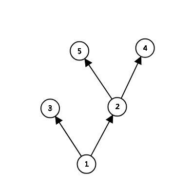
Figure 1: Example Graph


For example, if the vertex 1 is the source $S$, then the iteration count of vertex 1 is 1, the count of vertex 2 and 3 is 2, the count of vertex 4 and 5 is 3.


The random graph uses the configuration model described in [bollobas1980a] and [bender1978the]. For the node indexed $i\in[1,N]$, the degree sequence $d_{i}$ describe the count of the half-edges to be associated. Two half-edges will be paired uniformly to form an undirected edge. Though, it is assumed the performance on undirected random graph is similar to directed one. The degree sequence is given by $(d_{i})_{1}^{N}={\frac{M}{N}}$. For $W\in\mathbb{N}$, without loss of generality, the weights satisfy i.i.d.(identically distributed) distribution in $(-1,1)$. We assume the expectation of the weight is higher than 0, and the non-negative weights should occur with high probability(w.h.p.), because the often appearing negative weights will make it exist some negative cycles in averagely a constant neighborhood from $S$, making Raffica Algorithm solve in sublinear time complexity.



2.1 Bellman-Ford Algorithm


Bellman-Ford Algorithm[4] is a classic algorithm solving the SSSP on arbitrary weighted graph. It uses relaxing to iterate and after $N-1$ times iteration, we get the answer. If in the $N$th iteration there is any vertex relaxed, those vertices form negative cycle(s).


0:  Edges $E={u\to v,weight}$, Source $S$, Vertex count $N$, Edge count $M$



0:  Distance $dis$


  for $i=1\to N$ do




     $dis_{i}\leftarrow\infty$


  end for

  for $i=1\to N-1$ do




     for $i=1\to M$ do




        if $dis_{Edge_{i}.u}+Edge_{i}.w<dis_{Edge_{i}.v}$ then




           $dis_{Edge_{i}.v}\leftarrow dis_{Edge_{i}.u}+Edge_{i}.w$


        end if

     end for

  end for


The time complexity is obviously $O(MN)$. There are many kinds of improving methods like Yen’s, and so on. The following SPFA is also a kind of improving.




2.2 SPFA


SPFA is the queue optimized Bellman-Ford Algorithm.


SPFA uses a queue to keep the vertices, a little bit like BFS. SPFA uses Adjacency table. During the SPFA, we search and relax, pushing the relax-able vertices into the queue and update the distance.


The following pseudocode describes how SPFA works.





0:  Edges $E={u\to v,weight}$, Source $S$, Vertex count $N$, Edge count $M$



0:  Distance $dis$


  $queue\leftarrow S$


  for $i=1\to N$ do




     $dis_{i}\leftarrow\infty$


     $inqueue_{i}\leftarrow false$


     $dis_{S}\leftarrow 0,inqueue_{i}\leftarrow true$


  end for

  while queue is not empty do




     $x\leftarrow queue.front$


     queue.pop


     $inqueue_{x}\leftarrow false$


     for each E adjacent by x do




        if $dis_{E.u}+E.weight<dis_{E.v}$ then




           $dis_{E.v}\leftarrow dis_{E.u}+E.weight$


           if ($inqueue_{E.v}=false$) then




              $inqueue_{E.v}\leftarrow true$


              $queue\leftarrow E.v$


           end if

        end if

     end for

  end while





3 Raffica algorithm


Raffica algorithm is an improved SPFA.
Raffica algorithm is based on this theorem:



Theorem.


The solution of the SSSP forms a tree.




Proof.

Obviously the solution includes all the vertices reachable. Suppose the solution of the SSSP includes a cycle, and $X$ is a vertex on the cycle. It means if we go through the cycle from $X$ to $X$, the distance does not increase. If the sum of the weight of the whole cycle is positive, it will not be the SSSP, because going through this cycle will get a worse answer. If the weight of the cycle is zero, we need not go through this cycle. If negative, we will go through the cycle for infinite times, so that the answer does not exist. So the solution of SSSP does not include any cycles.




The method is pretty simple. Maintain the Auxiliary Tree. When relaxing an edge $E:u\to v$, we set $v$ as $u$’s son on the Auxiliary Tree $T$. If $v$ already has a father, we break the edge $v.father\to v$ on the Auxiliary Tree and reset $v.father$ as $u$. This operation is called ‘$Raffica\left(u,v\right)$‘. Then we successfully maintain a tree, except that $v$ is an ancestor of $u$ on the tree.


If $v$ is an ancestor of $u$ on the tree, this SSSP has a negative cycle $u\to...\to u$. When we can relax $E:u\to v$, it means $dis_{u}+E.w<dis_{v}$. If this inequality comes to a cycle during the iteration, it only means that there is a negative cycle. Therefore, the SSSP problem has no solutions. So what we maintain is absolutely a tree.


For the BFS can traverse all these vertices reachable, if there is a negative cycle reachable, we can absolutely find it.


So finding a cycle on the Auxiliary Tree is the necessary and sufficient condition of existing a reachable negative cycle.



Theorem.


Shortest Path(SP) can be divided into smaller SP. 



i.e. If SP $u\to v$ includes vertex $a$, we can conclude that $u\to a$ and $a\to v$ on the SP $u\to v$ are also SP in smaller problems.




During the iteration, suppose there is a vertex $u$ in the queue, and its ancestor $v$ is just Raffica-ed. Before Raffica-ed, $dis_{v}+\left(dis_{u}-dis_{v}\right)=dis_{u}$. $\left(dis_{u}-dis_{v}\right)$ means the length of the shortest path from $v$ to $u$. After Raffica-ed, $dis_{v}$ become lower, so $dis_{u}$ should become lower too, due to the Theorem 2nd.


For the vertex $u$ is still in queue, it uses an earlier distance data, so we can remove $u$ from the queue, else there will be redundant relaxing. So we clear the in-queue label of $v$’s subtree when $Raffica\left(u,v\right)$.





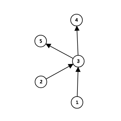
Figure 2: Example Graph 2


Consider the status of the picture. In a relaxation $1\to 3$, supposing 2 is the earlier father of 3. After $Raffica\left(1,3\right)$, 2 no longer has a child 3. Vertex 1 obtains a child 3.


Suppose that 4 and 5 are in queue at this time, we consider the updating $dis_{4}$ and $dis_{5}$. It is still using the old data. In other words, it still believe the best path is $2\to 3\to 4$ and $2\to 3\to 5$. But we have already known $1\to 3$ is better than $2\to 3$, so we should let 4 and 5 out of the queue, while 3 is in the queue, using the newest result, considering $1\to 3$ is the best. In the next iteration, 4 and 5 will consider $1\to 3\to 4$ and $1\to 3\to 5$ as the shortest path.


If we did not do this Raffica(i.e. SPFA), we will update 4’s son and 5’s son using $2\to 3\to 4$ and $2\to 3\to 5$ in the first iteration, and using $1\to 3\to 4$ and $1\to 3\to 5$ in the second iteration. If we would Raffica a lot in Raffica algorithm, and the SP Tree is tall, $SPFA$ will be very slow, because the new data will override the old data during every iteration. Although there is a lot of Rafficas, Raffica algorithm would not update all the subtree of SP Tree in average. It will update the subtree of Auxiliary Tree, which is not very tall.


In fact, it is common that a graph is done many Rafficas while having a tall SP Tree: a grid graph is one of the example, where SPFA runs slow and Raffica algorithm runs fast.


If we need to find out a negative cycle, we consider if v is the ancestor of v. If yes, there exists a negative cycle. We would simply use a DFS to check it, because DFS costs the same time as Raffica.


For random graphs, I use a different approach to make sure it is linear. It will be shown on Section 5.2.





0:  Edges $E={u\to v,weight}$, Source $S$, Vertex count $N$, Edge count $M$



0:  Distance $dis$


  $queue\leftarrow S$


  $T\leftarrow S$


  for $i=1\to N$ do




     $dis_{i}\leftarrow\infty$


     $inqueue_{i}\leftarrow false$


     $dis_{S}\leftarrow 0,inqueue_{S}\leftarrow true$


  end for

  while queue is not empty do




     $x\leftarrow queue.front()$


     queue.pop


     if $inqueue_{x}=false$ then




        continue


     end if

     $inqueue_{x}\leftarrow false$


     for each E adjacent by x do




        if $dis_{E.u}+E.weight<dis_{E.v}$ then




           $dis_{E.v}\leftarrow dis_{E.u}+E.weight$


           use a DFS to check if E.v is the ancestor of x


           if E.v is the ancestor of x then




              return  Exist a negative cycle


           end if

           Set it as false that the inqueue label on the vertices on the subtree rooted by E.v


           Clear the father-son relationship of all the vertices on the subtree rooted by E.v


           $T_{v}.father$ remove child $v$


           $T_{v}.fa\leftarrow x$


           if $inqueue_{E.v}=false$ then




              $inqueue_{E.v}\leftarrow true$


              $queue\leftarrow E.v$


           end if

        end if

     end for

  end while





4 Correctness


Raffica algorithm



Theorem.


For Raffica algorithm, the Auxiliary Tree is always a SP Tree of ‘the graph consist of all the vertices in Auxiliary Tree and the traversed edges‘. 



Proof.

I use a Mathematical Induction to prove it will return a correct answer.
Firstly, a tree consisted of a vertex obviously meets the condition.
Considering a relax, if it causes no Raffica, obviously it meets the condition. If it causes a $Raffica(u,v)$, the subtree of v is cut, it also meets the condition.




And now I am going to prove this algorithm will come to an end. Fist I prove a vertex cannot be Rafficaed more than N-2 times.
Consider a vertex $X$. Except the first time visited, because Raffica algorithm goes through the SP Tree, BFS costs $N-1$ iterations, which is the maximum possible height of SP Tree. For every iteration, only a vertex can Raffica $X$, because in a path from $S$ to a leaf, there is no more than one vertex in the queue.


After the Rafficas for every vertices, it remains a BFS. So absolutely the algorithm will come to an end.



5 Time Complexity



5.1 Worst Case


The worst case scenario of the Raffica algorithm is shown on the following picture:





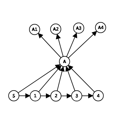
Figure 3: Worst case


Point A has $O(M)$ output and will be Raffica-ed $O(N)$ times. We may reconstruct the graph by spliting the output or randomizing. The worst case scenario time complexity can be improved to $O(\dfrac{MN}{\log N})$, but it is trivial.


In real life, there may be little vertices with $O(N)$ output like the above figure. In Section 8, I will show that this case can be improved. The unimprovable worst case scenario appears in a desperately extreme status, unlike the worst case of SPFA.









5.2 Random Graph


Raffica algorithm
A BFS is obviously $O(M)$, we consider the extra complexity caused by Raffica.


Firstly, the count of Raffica is no more than $M$(due to the correctness proof).


On the Auxiliary Tree, one’s ancestor can not be in queue with it. Suppose there is a leaf vertex $X$. $S\to X$ is a series of edges from root to leaf.



Theorem.


When an edge $E=\left(u,v\right)$ in the final SP tree is accessed, $u$ and $v$ will not be Raffica-ed. 



Proof.

There will not be any path shorter than the final SP Tree. Once it is accessed, there are no solutions better than this solution. So both $u$ and $v$ will not be Raffica-ed.




Due to [3], there is a property on the neighborhoods from $S$:






$$W_{n}(u,v)
-\frac{2\log\log N}{|\log(\tau-2)|}$$





$$H_{n}(u,v)
-\frac{2\log\log N}{|\log(\tau-2)|}$$





$$D_{n}(u,v)
-\frac{2\log\log N}{|\log(\tau-2)|},\tau\in(2,3)$$




are all tight sequence of random variables, which means they are convergent to 0 w.h.p.

Here $W_{n}(u,v)$ stands for the distance between $u$ and $v$ on a graph consist of $n$ nodes, where $u$ and $v$ are uniformly chosen in [1, n]. $H_{n}(u,v)$ stands for the hop-distance between $u$ and $v$(hop-distance is defined by the count of edges on the shortest path). $D_{n}(u,v)$ stands for the distance between $u$ and $v$ without consideration of weight. It shows that the vertices are mainly distributed in a small interval on the hop-distance and distance.

Due to [2], the diameter is $O(\log N)$.





Consider each path from the root to the leaf.
Basically, the density of Raffica is defined by the count of iterations between 2 Rafficas. The extra cost of $Raffica(u,v)$ is the size of the subtree rooted by $v$. The total cost of the Raffica operation is the sum of all the extra costs.




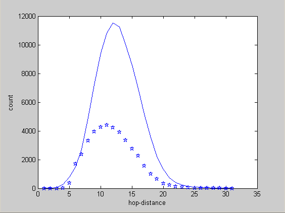
Figure 4: N = $10^{5}$, M = $10^{6}$


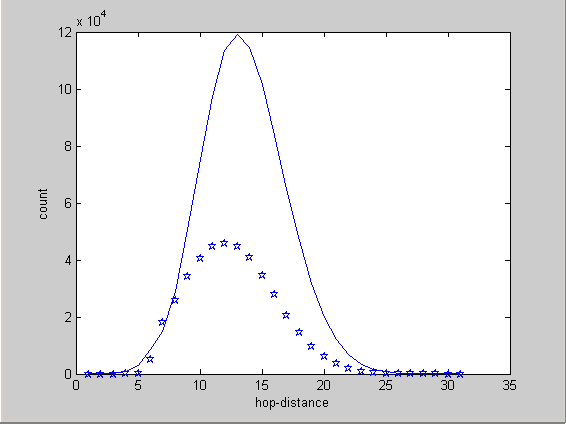
Figure 5: N = $10^{6}$, M = $10^{7}$


The figure 4 and 5 are my test cases. The solid curve is the count of x-depth vertices, while the dotted curve is the count of Raffica on x-depth.




Basically, the density of Raffica on a sparse graph is $O(\dfrac{1}{\log N})$ w.h.p. It is not very good for my algorithm. Now I introduce my improvement mentioned above.



Theorem R.


Suppose the density of Raffica is a constant w.h.p., our algorithm should be linear in expectation.




Therefore, the improvement is:


For it is a random graph, we can predict the average distribution of x-depth vertices and x-depth Raffica counts before the algorithm. We randomly add some Raffica due to the distribution, so that the density tends to 0.5 in probability. More precisely, we select some edges that cannot fit the triangle inequality during the iteration, and disassemble its subtree. The two vertices connected by the edge should be on the adjacent depth. Those chosen edges would be Rafficaed due to the selection of probability.


It seems that adding more Raffica will simply make the algorithm slower. However, it cuts down the average size of the subtree, making its total average time shorter.


Proof of Theorem R


Denote the count of vertices that is on the i-depth from S as $\Gamma_{i}(S)$, and $\Gamma^{\prime}_{i}(S)=\dfrac{\Gamma_{i}(S)}{\Gamma_{i-1}(S)}$. Easily, $\Gamma^{\prime}_{i}(S)$ is monotone decreasing with variable $i$.





Lemma 1.


$\mathbb{P}(\Gamma^{\prime}_{dis_{u}}(S)<\epsilon_{0})=1$, for any $\epsilon_{0}>1$ and $u$ uniformly chosen in $[1,N]$.




Proof.

Due to [Adriaans2017Weighted], $dis_{u}$ tends to infinity w.h.p.
$T_{a}(i)$ was defined by the radius of the ball centered by $S$ that contains $k$ vertices. More precisely,




$$T_{a}(i)=r|\{x\in[1,N]|dis_{x}<=r\}|=i$$



According to [CornellThe], for $\alpha_{N}=\lfloor\log^{3}N\rfloor$, $\beta_{N}=\lfloor\sqrt{\dfrac{\mu}{v-1}N\log N}\rfloor$(two balls of size at least $\beta_{N}$ intersect almost surely), $\alpha_{N}\leqslant i\leqslant\beta_{N}$, some constant number $v,\epsilon,\mu$, define $\rho=\dfrac{v-1}{1+\epsilon}$,




$$T_{a}(i+1)-T_{a}(i)
\leqslant e^{\frac{v-1}{1+\epsilon}i}$$






$$=i^{3\rho}$$



For $\Gamma^{\prime}_{i}(S)$ is monotone decreasing with $i$, $T_{a}(i)$ is monotone increasing with $i$. We would only consider $T_{a}(\alpha_{N})$, for the corresponding $\Gamma^{\prime}_{depth_{i}}$ is largest. Its inverse function is:




$$T_{a}^{-1}(i)=i^{\frac{1}{3\rho}}$$



The inverse function satisfies $T_{a}^{-1}(i)\propto\Gamma_{depth_{i}}$. Therefore,




$$i
=\alpha_{N}$$





$$\Gamma^{\prime}_{depth_{i}}
=\frac{\Gamma_{depth_{i}}}{\Gamma_{depth_{i}-1}}$$






$$=\frac{T_{a}^{-1}(i)}{T_{a}^{-1}(i-1)}$$





$$=\frac{i^{\frac{1}{3\rho}}}{(i-1)^{\frac{1}{3\rho}}}
=1$$




Meanwhile, $\mathbb{P}(dis_{u}<T_{a}(\alpha_{N}))=0$; when $dis_{u}>T_{a}(\beta_{N})$, $\Gamma^{\prime}_{depth_{i}}<1$. Q.E.D.






The expecting time of Raffica is:




$$T_{Raffica}(N)
=O(M/N*\sum_{i=1}^{N}\frac{\Gamma_{depth_{i}-2}(S)}{\Gamma_{depth_{i}}(S)})$$






$$\leqslant O(M/N*N*\max{\frac{\Gamma_{depth_{i}-2}(S)}{\Gamma_{depth_{i}}(S)}})$$





$$=O(M/N)*O(N)$$





$$=O(M)$$







It is worth mentioning that this optimization should not work better than the original one on small test cases. This optimization always makes the enter-queue count tend to $O(M)$, while the original one makes the enter-queue count tend to $O(M\log N)$. The factor under the signal $O$ causes this phenomenon.


Now we know that the total cost by Raffica is $O(M)$. The question turns out to be how much time does other operations cost. It looks like very slow to check and update a subtree of $E.v$, because each DFS may cost $O(M)$. However, the subtree to be maintained and to be checked, is the same size as Raffica operator, making the other operations using DFS the same cost as Raffica. The conclusion is, Raffica Algorithm has $\Theta(M)$ time complexity in expect on random graph.




SPFA For SPFA, I give an upper bound. The difference between $SPFA$ and Raffica algorithm is SPFA does not clear the in-queue label of the subtree of the Dark Point. According to [2], the diameter of a random graph is $D=O(\log N)$. The upper bound is $O(M\log N)$.


When SPFA deals with negative cycle, its expect time complexity is $\Theta(MN)$, while Raffica algorithm is $\Theta(M)$. Because SPFA judges a negative cycle by checking how many times any vertices be in queue. If one enters the queue $N$ times, there turns out to be a negative cycle. For each iteration, there are totally expecting $\Theta(N)$ vertices in queue. Raffica algorithm gets the existence of a negative cycle when it traverses a negative cycle. Therefore, the time complexity is $\Theta(M)$.









5.3 Traffic Problem or Grid Graph


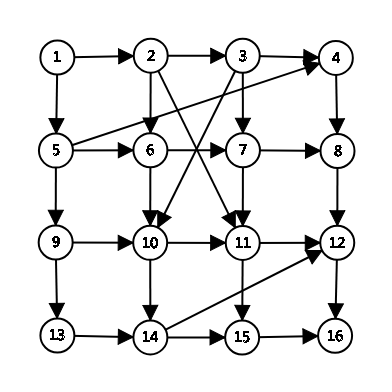
Figure 6: A grid graph


Now we consider a grid or a near-grid graph. The diameter of these graphs are $\Theta(N)$, and the counts of out degrees are $O(1)$. The weights of the edges satisfy the same distribution as the model of above random graph. A grid graph or near-grid graph is often seen in real life. I call it a traffic problem.


SPFA runs slow in this graph, while Raffica algorithm runs in linear complexity.


Using a similar way, when $N$ tends to infinity, the density of Raffica is made to be $0.5$. In the same way, the time is $\Theta(M)$.


Consider SPFA. The diameter of the grid graph is $\Theta(N)$, therefore the time of Raffica is $\Theta(N)$. The density of Raffica tends to $\widetilde{O}(1)$. The total cost is $\Theta(N)*\Theta(N)*\widetilde{O}(1)=\widetilde{\Theta}(N^{2})$ in expect.


In fact, SPFA’s time complexity depends on the height of the SP tree and the density of Raffica. Actually, the grid graph is not the only one of the graphs that SPFA runs slow. If both the height and the density are huge, SPFA also runs slow. This status often appears in traffic SSSP problems.



6 Comparison


Table 1: SSSP




Dijkstra(Fib Heap)
Bellman-Ford
SPFA
Raffica
Thorup[27]



Non-negative weighted Random Graph
$O(M+N\lg N)$
$O(MN)$
$O(MD)$
$O(M)$
$O(M)$


Worst Case
$O(M+N\lg N)$
$O(MN)$
$O(MN)$
$O(MN)$
$O(M)$


Negative Cycle
Random Graph
unable
$O(MN)$
$O(MN)$
$O(M)$
unable


Arbitrary Weight
Random Graph
unable
$O(MN)$
$O(MD)$
$O(M)$
unable


Traffic Problem

$O(M+N\lg N)$
$O(MN)$
$O(MN)$
$O(M)$
$O(M)$


Directed Graph
able
able
able
able
unable





Table 2: APSP




Hagerup[20]

Floyd
SPFA
Raffica
Thorup


Non-negative Weighted Random Graph
$O(MN+N^{2}\lg\lg N)$
$O(N^{3})$
$O(MND)$
$O(MN)$
$O(MN)$


Worst Case
$O(MN+N^{2}\lg\lg N)$
$O(N^{3})$
$O(N^{2}M)$
$O(N^{2}M)$
$O(MN)$


Arbitrary Weight
Random Graph
$O(MN+N^{2}\lg\lg N)$
$O(N^{3})$
$O(MND)$
$O(MN)$
unable


Directed Graph
able
able
able
able
unable





I use two tables to compare the performance of some classical algorithms and my algorithm on SSSP and APSP.


In random graph or traffic problem, Raffica algorithm has linear complexity, which is absolutely fastest. Thorup’s algorithm is also linear, which should be the fastest too. But it can only handle undirected graph, and it is very complex.



7 Applications



7.1 System of Difference Constraints


System of Difference Constraints is a problem handling a series of inequality $X_{i}-X_{j}<k$. It can be easily transformed to a SSSP problem. It is widely used to many applications, such as temporal reasoning.


Set a vertex S as the super source vertex. Transform the inequality $X_{i}-X_{j}<k$ to $X_{i}+\left(-k\right)<X_{j}$. For each inequality, add an edge $X_{i}\to X_{j}$ with weight $-k$. For each vertex X, add an edge $S\to X$ with weight 0. Then regard S as source, the solution of System of Difference Constraints is the solution of SSSP. If there exists any negative cycle, the solution does not exist.


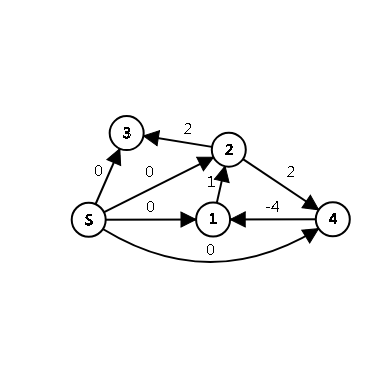
Figure 7: System of Difference Constraints


The above graph stands for these constraints:




$$x_{1}-x_{2}
<-1$$





$$x_{2}-x_{3}
<-2$$





$$x_{2}-x_{4}
<-2$$





$$x_{4}-x_{1}
<4$$








This system has no solutions because $1\to 2\to 4\to 1$ is a negative cycle.





We want to know if this problem has any solutions. Therefore we want to find if this SSSP problem has a negative cycle.


Bellman-Ford Algorithm and SPFA cannot solve the find-negative-cycle problem very fast. If the problem is random one, Raffica algorithm can solve it in linear time.




7.2 Detecting the minimum average weight cycle


An average weight of a cycle denotes the total sum of the weights of the cycle divided by the total count of the cycle. Karp’s algorithm[21] solves it in $O(MN)$. If the graph can be regarded as a random graph, Raffica algorithm can solve it in $O(M\lg W)$($W$ stands the max weight of the edges) by a simple dichotomy.



8 Open problem


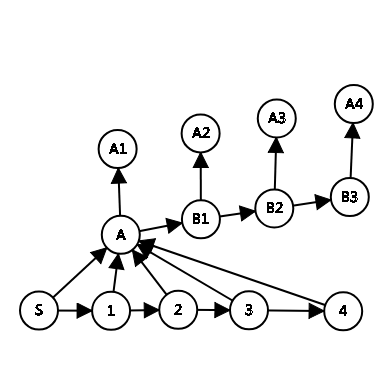
Figure 8: Reconstructed Worst case


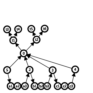
Figure 9: Worst case that can hardly be reconstructed


Figure 8 is the worst case scenario. This case may often appear in real life. We can easily transform it to the figure 6 scenario. For the vertex with many out degrees, we separate these edges into those vertices. It is easy to see the correctness of the transformation. And it is easier(linear) to solve by Raffica algorithm.





Figure 9 is another status. The 0 vertex has a subtree looked like a binary-tree. We cannot handle it like the upper one. But we can hardly see it in real life. What we can do is to change the method of searching: not BFS or DFS, but an IDFS. I cannot quantitative the effect of this optimization yet.


In conclusion, if there is a vertex with a subtree on the SP Tree having $O(N)$ vertices in a particular depth, and we visit it in a particular way, so that those $O(N)$ vertices updated many times. And that is the worst case.


Another feature of the worst case is: there are some vertices visited many times. But even if we separate the in-degree, the in-degree may also appear like a binary-tree.


In this way, we can separate the in-degree and out-degree, improving the worst case to $\Theta(MN/\log N)$. Reconstructing the graph remains an open problem.


We can also use priority queue to improve the worst case. Using an evaluation function, we can let it have a higher priority where the size of sub-tree is small. It can solve the binary-tree status, but it can not tackle all the statuses.



9 Acknowledgments


I would like to acknowledge Mr.Wang, Mr.Wen and anyone who has supported me, and those who used this algorithm to real problem settling, giving me priceless test cases and examples. Thanks to Prof.Andrew for informing me my algorithm is very similar to Tarjan’s unpublished algorithm, to Prof.Tarjan for pointing out my theoretical mistakes. Thanks to Mr.Zhou for checking language mistakes.

References

[1]
R. K. Ahuja, K. Mehlhorn, J. Orlin, and R. E. Tarjan.
Faster algorithms for the shortest path problem.
Journal of the ACM (JACM), 37(2):213–223, 1990.
[2]
H. Amini and M. Lelarge.
The diameter of weighted random graphs.
Annals of Applied Probability, 25(3):p gs. 1686–1727, 2012.
[3]
E. Baroni, R. van der Hofstad, and J. Komjathy.
Tight fluctuations of weight-distances in random graphs with
infinite-variance degrees.
2016.
[4]
R. Bellman.
On a routing problem.
Quarterly of Applied Mathematics, 16(1):87–90, 1958.
[5]
Y. Boykov, O. Veksler, and R. Zabih.
Fast approximate energy minimization via graph cuts.
IEEE Transactions on Pattern Analysis and Machine Intelligence,
23(11):1222–1239, 2002.
[6]
K. Chatterjee, M. Henzinger, S. Krinninger, V. Loitzenbauer, and M. A. Raskin.
Approximating the minimum cycle mean .
Theoretical Computer Science, 547(1):104–116, 2014.
[7]
B. V. Cherkassky, L. Georgiadis, A. V. Goldberg, R. E. Tarjan, and R. F.
Werneck.
Shortest-path feasibility algorithms:an experimental evaluation.
Journal of Experimental Algorithmics,
14(12):124312–124312–11, 2010.
[8]
B. V. Cherkassky and A. V. Goldberg.