Investigation of the orientation of galaxies in clusters: the importance, methods and results of research
Abstract
Various models of structure formation can account for various aspects of the galaxy formation process on different scales, as well as for various observational features of structures. Thus, the investigation of galaxies orientation constitute a standard test of galaxies formation scenarios since observed variations in angular momentum represent fundamental constraints for any model of galaxy formation. We have improved the method of analysis of the alignment of galaxies in clusters. Now, the method allows to analyze both position angles of galaxy major axes and two angles describing the spatial orientation of galaxies. The distributions of analyzed angles were tested for isotropy by applying different statistical tests. For sample of analyzed clusters we have computed the mean values of analyzed statistics, checking whether they are the same as expected ones in the case of random distribution of analyzed angles. The detailed discussion of this method has been performed. We have shown how to proceed in many particular cases in order to improve the statistical reasoning when analyzing the distribution of the angles in the observational data. Separately, we have compared these new results with those obtained from numerical simulations. We show how powerful is our method on the example of galaxy orientation analysis in 247 Abell rich galaxy clusters. We have found that the orientations of galaxies in analyzed clusters are not random. It means that we genuinely confirmed an existence of the alignment of galaxies in rich Abells’ galaxy clusters. This result is independent from the clusters of Bautz-Morgan types.
1 Introduction
Solving the problem of the structures formation is one of the most significant issue of modern extragalactic astronomy. Many authors investigated the scenarios of structures formation since Peebles (1969); Zeldovich (1970). New scenarios are mostly modifications and improvements of the older ones (Lee & Pen, 2000, 2001, 2002; Navarro at al., 2004; Mo et al., 2005; Bower et al., 2006; Trujillio et al., 2006; Brook et al., 2008; Paz at al., 2008; Shandarin et al., 2012; Codis et al., 2012; Varela et al., 2012; Giahi-Saravani & Schaefer, 2014; Blazek et al., 2015).
The final test of veracity in a given scenario is the convergence of its predictions with observations. One of the possibilities of such test is analysing the angular momenta of galaxies. Investigating the orientation of galaxy planes in space is of great importance since various scenarios of cosmic structures formation and evolution predict different distributions of galaxies angular momentum, (Peebles, 1969; Doroshkevich, 1973; Shandarin, 1974; Efstathiou & Silk, 1983; Catelan & Theuns, 1996; Li, 1998; Lee & Pen, 2000, 2001, 2002; Navarro at al., 2004; Trujillio et al., 2006; Zhang et al., 2013), i.e. provide distinct predictions concerning the orientation of objects at different levels of structure – in particular clusters and superclusters of galaxies. Our model assumes that normals to the planes of galaxies are their rotational axes, which seems to be quite reasonable, at least for the spiral galaxies. Various models can account for various aspects of the galaxy formation process on different scales, as well as for various observational features of structures. This provides us with a method for testing scenarios of galaxy formation. In other words, the observed variations in angular momentum give us simple but fundamental test for different models of galaxy formation (Romanowsky & Fall, 2012; Joachimi et al., 2015; Kiessling et al., 2015).
From the observational point of view it is not very difficult to investigate the distribution of the angular momenta for the luminous matter i.e. real galaxies and their structures. One should note however, that in real Universe, observed luminous matter of galaxies are surrounded by dark matter halos that are much more extended and massive. Direct observation of dark mater halos and theirs angular momentum is not so easy. Fortunately, there are the relation between luminous and dark mater (sub)structures. As a result we have a dependence between dark matter halos and luminous matter (real galaxies) orientation (Trujillio et al., 2006; Paz at al., 2008; Pereira et al., 2008; Bett et al., 2010; Paz et al., 2011; Kimm et al., 2011; Varela et al., 2012). Recently, the analysis of the Horizon-AGN simulation shows the similar dependence (Okabe et al., 2018; Codis et al., 2018). It means that the analysis of angular momentum of luminous matter gives us also information about angular momentum of the total structure hence the analysis of the angular momentum of real (luminous) galaxies is still useful as a test of galaxy formation. The investigation of the galaxies orientation in clusters are also very important with regard to investigation of weak gravitational lensing For more detailed discussion of the significance of this problem see Heavens et al. (2000); Heymans et al. (2004); Kiessling et al. (2015); Stephanovich & Godłowski (2015); Codis et al. (2016).
Since the angular momenta of galaxies and also the directions of galaxy spin are usually unknown, the orientations of galaxies are investigated instead. In order to acquire this, either the distributions of galaxy position angles only (Hawley & Peebles, 1975) or the distributions of the angles giving the orientation of galaxy planes (Jaaniste & Saar, 1978; Flin & Godłowski, 1986) are examined. Many authors investigated the orientation of galaxies in different scales. The review of the observational results on the problem of galaxies orientation and structures formation was presented both theoretically (Schaefer, 2009) and observationally (Godłowski, 2011a; Romanowsky & Fall, 2012).
One of the most meaningful aspects of the problem of the origin of galaxies involves the investigation of the orientation of galaxies in clusters. During the analysis of the angular momentum of a galaxy cluster, in principle we should take into account that total angular momentum of the cluster could come from both the angular momentum of each galaxy member and from the rotation of the cluster itself. However, one should note that there is no evidence for rotation of the groups and clusters of galaxies themselves. So, it is commonly agreed that such structures do not rotate (for example Regos & Geller (1989); Diaferio & Geller (1997); Diaferio (1999); Rines et al. (2003); Hwang & Lee (2007); Tovmassian (2015), see however Kalinkov et al. (2005) for the opposite opinion). An especially important result is obtained by Hwang & Lee (2007). They have examined the dispersions and velocity gradients in 899 Abell clusters and have found a possible evidence for rotation in only six of them. This allowed us to conclude that any non-zero angular momentum in groups and clusters of galaxies should arise only from possible alignment of galaxy spins. Moreover, the stronger alignment means the larger angular momentum of such structures.
For many years, astrophysisicts payed a lot of attention to the orientation of galaxies in clusters. It was investigated both theoretically (see for example (Ciotti & Dutta, 1994; Ciotti & Giampieri, 2008)) and observationally. Generally, summarizing the research results provided by various authors, it can be stated that we have no satisfactory evidence for the alignment of galaxies in groups and poor clusters of galaxies, while there is an ample evidence of this kind for rich clusters of galaxies (Godlowski et al., 2005) (see also Godłowski (2011a) for an improved analysis and Stephanovich & Godłowski (2015) for review).
Thus, an interesting problem arises if there are any dependence on the alignment to the mass of the structure. Godlowski et al. (2005) suggested that the alignment of galaxies in clusters should increase with the mass of the cluter. Thus, Godlowski et al. (2005) hinted that the alignment should increase with the number of objects (richness) in a particular cluster, too. These suggestions were later confirmed by Aryal (2007). These autors analyzed a total of 32 clusters of different richness and BM types. They confirmed that the alignment is changing with the richness and moreover that they change with BM type of the clusters. However, one should note that both Godlowski et al. (2005) and Aryal (2007) investigations were qualitative only. The next step is to test this hypothesis also quantitatively.
This was the reason why Godłowski et al. (2010) examined the orientation of galaxies in clusters both qualitatively and quantitatively. In this paper it was found that the alignment of galaxy orientation increased with numerousness of the cluster. However, the problem that we may obtain is whether we found a significant alignment in analyzed sample of 247 rich Abell clusters, or increasing alignment with cluster richness only. For this reason Godłowski (2012) analyzed the distribution of position angles using test, Fourier test and autocorrelation test as well as Kolmogorov test, showing that it is not random.
In the present paper, following the ideas of Godłowski (2012) and Panko et al. (2013), we improved method allows us to analyze the distributions both of the position angles and distribution of two angles giving spatial orientation of galaxies. We denote angle (the polar angle between the normal to the galaxy plane and the main plane of the coordinate system) and the angle (the azimuth angle between the projection of this normal onto the main plane and the direction towards the zero initial meridian), see Figure 1 for geometry of the angles. The main idea of our method is to analyze the distributions of these angles using statistical tests. We have analyzed in more details and improved the statistical tests used in (Godłowski, 2012) as well as introduce new statistical tests into the method. We analyzed how the tests changes if expected values of galaxies in particlular bins varies (as in the case of analysis of the angle). It slightly changes for autocorelation test but it is very important for Fourier test and Kolmogorov-Smirnov test. We also introduced to our improved method of investigation of galaxy alignment in clusters, the ”control tests” that neglects a possible asymmetry of the distribution according to main coordinate plane. The idea of such tests is to analyze only the difference between more ”parallel” or more ”perpendicular” orientation according to the coordinate system main plane (or main direction towards the zero initial meridian in the case angle). We have checked how the Kolmogorov-Smirnov test behaves in the investigation of the orientation of galaxies in cluters. We have introduced alternative tests, namely Crámer-von Mises and Watson that showed more explicitly that the allignment truly exists.
Usually the effect of aligment of galaxies in structures is not very strong and its analysis requires precise statistical considerations. In such a case it is very important to verify that no other observational systematics can affect. To avoid a problem with the possible impact on the obtained results by data systematics, we think it is necessary to test the method on a well-tested sample of galaxy clusters. We have decided to use a sample of the galaxy clusters selected on the basis of the PF catalog (Panko & Flin, 2006). Hence, on the example of analysis of position angles in 247 rich Abell clusters we show how the method works in case of observational data. For our sample of 247 clusters, we computed the mean values of the analyzed statistics. Our null hypothesis is that the mean value of the analyzed statistics is as expected in the case of random distribution of analyzed angles. At first, we have compared the theoretical prediction with the results obtained from numerical simulations. Later, they are compared with the results obtained from the real sample of the 247 Abell clusters. Separately, we analyzed the sample when only galaxies brighter than were considered. Moreover, we decided to analyze if there are any differences in alignment of galaxies in the clusters belonging to different Bautz-Morgan (BM) types. In order to exclude the case that the obtained results comes from errors in observational measurements, we have used two separate methods. We have analyzed the sample assuming random errors in position angles and additionaly we have used jackknife method especially to investigate the possible influence of background objects.
The novelty of our approach is to gather many methods of analysis of statistics of all angles , and not only for some particular galaxy clusters but also for big samples of clusters. Unfortunately, such approach inevitably turns to the analysis on a case by case basis. That is why in each case, we point out possible difficulties and show which method has to be used. At first glance, most cases looks very similar, but one has to be careful not to omit the crucial differences. The advantage of the approach is that by analysing much more data at once, we are able to draw more general conclusions.
2 Observational data
In the present paper we have analyzed the sample of 247 rich Abell clusters containing at least 100 members galaxies each (Godłowski et al., 2010; Godłowski, 2012). The sample was selected on the basis of the PF catalogue (Panko & Flin, 2006). The structures in the Panko & Flin (2006) catalogue were extracted from the Muenster Red Sky Survey (MRSS hereafter) (MRSS, 2003) using the 2D Voronoi tessellation technique (Ramella et al., 2001), see Panko et al. (2009) for details. Note that the confidence level for cluster search was (Ramella et al., 2001) and the list of clusters is reliable.
During analysis of the orientation of galaxies in structures the curcial point is to remove the non-galactic objects - mostly stars and artifacts. The advantage of MRSS list of galaxies is that the author of the catalogue very carefully analyzed the classification of all objects in the survey. Basic data for MRSS are 217 ESO Southern Sky Atlas R Schmidt plates covering an area of about 5000 square degrees in the southern hemisphere, with . All plates were digitized with the two PDS 2020GMPlus microdensitometers of the Astronomisches Institut Münster with a step width of 15 microns (1600 dpi), corresponding to arcseconds per pixel. Objects search in digitized plates was made using the program SEARCH based on FOCAS algorithm (Jarvis & Tyson, 1981), see also Ungruhe (1997); MRSS (2003) for detailed aplication to MRSS catalogue. The analysis of variations of background densities, in particular vignetting of the telescope, and the influence of threshold of the background for the objects detection were made carefully. The influence of nearest objects was minimized due to final analysis inside the small frame including the object. Final galaxy search based on 6 parameters allows to select only galaxies. More than 2700000 uncertain objects were checked visually; they were faint objects mainly (MRSS, 2003). So, all selected objects are galaxies.
Resulting list of MRSS galaxies contains more than 5 millions ones till to detected on the best plates. However, the limit of completeness of MRSS is (MRSS, 2003). This short list contains 1200000 galaxies with reliable definitions parameters. The ellipticity and position angle for each galaxy were calculated using the covariance ellipse method ((Carter & Metcalf, 1980)). The ellipticities and positional angles of galaxy images were calculated using both intensities and coordinates, so inside intensity distribution was accounted (MRSS, 2003). The problem of possible systematic effects was analyzed by Ungruhe (1997); MRSS (2003) while the detailed study of uncertainties on the position angles, including vary with galactocentric distance, was executed in Biernacka & Flin (2011). They confirmed the results of Nilson (1974). Following the results, we supposed the uncertainties on the position angles of galaxies on the level for galaxies elongated images of galaxies, in the worst case the uncertainties were on the level . Obviously the uncertainties quickly increase for rounded images.
The PF Catalogue was created using only MRSS galaxies inside the completeness limit . The PF Catalogue defines a cluster as a structure which contains at least ten galaxies in the magnitude range between and , where is the magnitude of the third brightest galaxy located in the considered structure region. The criterion of is a well known criterion to galaxy membership for the cluster if, as in the case MRSS (2003) we have no information about radial velocities of particular galaxies. Panko et al. (2009) checked the correctness of this limit using statistical completed sample contained 547 PF structures.
The full PF (Panko & Flin, 2006) catalogue includes 6188 galaxy clusters and groups and contains positions of the clusters, their radii, areas, the number of all galaxies in the field of structure, number of galaxies within the magnitude range and , as well as an estimated number of background galaxies, ellipticity and position angles for each structure, magnitudes of the first, the third and the tenth galaxy in a structure (taken from the MRSS). The full PF catalogue contains not only the list of the clusters but also the lists of galaxies belonging to each structures, where the data for each galaxy member were taken from the MRSS. This data includes: the equatorial coordinates of galaxies (, ), the diameters of major and minor axes of the galaxy image ( and respectively) and the position angle of the major axis (see also Godłowski (2012)). Because the position angles in MRSS serve in clockwise system, we recomputed original position angles from MRSS clockwise system to standard counterclockwise system. We performed our computation in Equatorial and Supergalactic Coordinate System defined in Flin & Godłowski (1986). In the case of Supergalactic Coordinate System position angles were recomputed to supergalactic position angles . The photometrical redshifts were calculated for each cluster using the relation (Biernacka et al. (2009)) and rich PF clusters have redshifts while median z=0.08. The positions of PF and APM (Dalton at al., 1997) galaxy clusters are in good agreement (Biernacka et al., 2009).
In the present paper, as in Godłowski et al. (2010) and Godłowski (2012) we have analyzed the sample of rich clusters that have at least 100 members and belong to ACO clusters (Abell et al., 1989). The advantage of such sample is that they have the Bautz–Morgan morphological types (BM types). There are 239 such objects in the PF catalogue. Moreover, 9 objects can be identified with two ACO clusters. We decide to include them in our investigation and increased our sample to 248 objects. We excluded the structure A3822, which potentially has substructures (Biviano et al., 1997, 2002). Therefore, finally our analyzed sample contains 247 clusters. Because all analyzed clusters have ACO identification, the distances can be found from literatures or extrapolated from 10th brightest galaxy in clusters (Panko & Flin, 2006; Biernacka et al., 2009). The numbers of clusers with particular BM types are from (BM I) till (BM II).
In our investigation we have decided to analyze two subsamples of data. The first one contains all galaxies lying in the region regarded as cluster. In the second one, for avoiding possible role of background object, only galaxies brighter than were taken into account.
3 The method of investigation
The analysis of the orientation of galaxies has usually been examined by two main methods. In the first one (Hawley & Peebles, 1975) the distribution of the position angles of the major axis of galaxies is performed. During the analysis of position angles, we exclude from examination all galaxies with axial ratio , because for the face–on galaxies position angles give only marginal information connected with the orientation of galaxy. In the second method based on the de–projection of the galaxy images, we have analyzed spatial orientation of galaxies. This idea was introduced by Oepik (1970), applied by Jaaniste & Saar (1978) and significantly modified by Flin & Godłowski (1986); Godłowski (1993a, 1994a). In this method, we take into account both galactic position angles and another important parameter – the galaxy inclination with respect to the observers’ line of sight . Using these two angles we have determined two possible orientations of the galaxy plane in space, which gave two possible directions perpendicular to the galaxy plane. As was discussed in the introduction, it is expected that one of these normal corresponds to the direction of galactic rotation axis. One should note however, that de–projection of galaxy images on the celestial sphere gives four solutions for the angular momentum vector. Usually we consider only two distinguishable solutions since we do not know the direction of galaxy rotation.
The inclination angle has been computed from the galaxy image according to the formula: , where the observed axial ratio and is ”true” axial ratio. This formula is valid for oblate spheroids (Holmberg, 1946). The value is used in the case when we have no information about morphological types of galaxies (as in MRSS catalog). For each galaxy we determined two angles and . Following Godłowski (2012) we performed our computation both in Equatorial and Supergalactic coordinate systems (Flin & Godłowski (1986) based on Sandage & Tammann (1976)). The relations between angles (, ) and (, ) in the Supergalactic coordinate system (, ) (Figure 1) are the following ones (similar formulae may be obtained for Equatorial coordinate system)
| (1) |
| (2) |
| (3) |
where . As a result of the reduction of our analysis into two solutions only, it is necessary to consider the sign of the expression: and for we should reverse the sign of respectively (see Godłowski et al. (2010)). Please note the usualy the researchers use the simplified version of the method, taking into account only Equations 1 and 2, which however caused serious problems in the interpertation of the results of the analysis of the spatial orientation of galaxies.
The essential progress of the investigation of galaxy alignment was made by Hawley & Peebles (1975). Their method of investigation of galaxies orientation is based on statistical analysis of the distribution of galaxies position angles. The essence of the method was to use three type of statistical tests: -test, Fourier and First Autocorrelation. It was shown later that this methodology can also be used to study the spatial orientation of galaxies planes (Flin & Godłowski, 1986; Kindl, 1987; Aryal & Saurer, 2000; Godłowski et al., 2010; Panko et al., 2013; Yadav et al., 2016).
The main idea of the paper is to show how to make the statistical methods more reliable and to interpret the obtained results. We show how the methods work in particular cases and apply it to the analysis of the distribution of position angles of observational sample of 247 rich Abell clusters. In particular we determine if the orientations of galaxies in clusters are isotropic or not.
The essence of the method Godłowski (2012) is to compute the mean values of analyzed statistics for the whole sample of analyzed cluster and compare them with that obtained from numerical simulations. Our null hypothesis is that the mean value of the analyzed statistics is as expected in the case of random distribution of analyzed angles. In all tests, the range of the angle (where for one can put , , (or ) respectively) is divided into bins of equal width. We have used bins. As a check, we repeated the division for other values of , but generally we have not found any significant difference. There is one exception, namely is Kolmogorov-Smirnov test and we discuss this in detail in the section ”Numerical Simulations and Results”.
In the whole paper we denote as the total number of galaxies in analyzed clusters while is the number of galaxies with orientations within the -th angular bin and is the expected number of galaxies in the k-th bin. In the case of the analysis of the position angles or and angles all are equal to , which is also the mean number of galaxies per bin. In the case of the analysis of the angles of course are not equal and are obtained from the cosine distribution. The case when not all are equal was not analyzed in the paper of Godłowski (2012), so adding such analysis significantly improves the method of analyzing the alignment of galaxies in clusters. This improvement means that the method is now valid also in the case when some (or even all) bins have not equal width.
The first group of tests is based on the test:
| (4) |
where is the probability that a chosen galaxy falls into -th bin. Because we have bins, the number of degrees of freedom of the test is . This causes that the mean value and the variance . For this leads to the values and . When we analyzed the sample of clusters and computed the mean value of statistic, then , but decreased by the factor and equaled . For and this gives and .
In the basic investigation the range of angle is from to . The idea of the control test is to restrict our analysis only to the case of the absolute value of angle (Flin & Godłowski, 1986; Aryal, 2004; Aryal & Saurer, 2005a; Aryal, 2006, 2007). Then, we neglected a possible asymmetry of the distribution according to main coordinate plane and analyzed only the differences between more ”parallel” or more ”perpendicular” orientation according to the coordinate system main plane. So the range of angle is from to and we divided the entire range of a angle into instead of bins. During the analysis of clusters the mean value of statistic is of course while and . Analogically, during analysis of the position and azimuthal and angles, we also reduced ranges of analyzed angles from to , so we divided the entire range of a angle into instead of bins. Of course in the case of angle, the idea of the control test is to analyze the asymmetry between more ”parallel” or more ”perpendicular” projection to the normal to the galaxy plane according to the main direction towards the zero initial meridian of the coordinate system.
The second group of our tests is based on the first auto-correlation test (Hawley & Peebles, 1975). Probably the best test for autocorrelation is the von-Neumann-Durbin-Watson test. However, in our paper we do not analyse full autocorrelation. Our idea is, as noted above, to obtain the average value for analysed statistic (and later to check if the mean value of the analysed statistics is as expected in the case of random distribution of analysed angles). Although, the Hawley & Peebles (1975) first autocorrelation test may not work as well as the von-Neumann-Durbin-Watson test, the idea presented there is also widely used (see for example Percival & Walden (1993)- especially Chapter 6 of the book). So, it seems that the use of this test works well enough. However, we analyzed its properties in more detail than Hawley & Peebles (1975) before we used it.
The first auto-correlation test quantifies the correlations between galaxy numbers in neighboring angle bins. This correlation is measured by the statistic :
| (5) |
where . According to the original paper Hawley & Peebles (1975), in the case of an isotropic distribution, the expected value of is with the standard deviation .
In the paper Godłowski (2012), it was shown that original Hawley & Peebles (1975) result was an approximation only that is not correct in our case, since they assumed that are independent from each other. Therefore, in the formula for is present an additional term connected with the covariance between and :
| (6) |
When all and hence are equal (), as it was in the case of position angles, then . Moreover, contains a term which is the variance of the products of and which are not independent. As a result, the correct value of is only approximately equal to and the correct value must be computed using numerical simulations. Moreover, for one cluster the difference between the results in expected values of (0 or -1) is relatively small compared to . However, when we analyse the sample of clusters, the situation is different because the variance is decreased by the factor . As a result, in the case of sample clusters, is significantly smaller than (which is the difference between expected values) (Godłowski, 2012).
In the case of analysis of the angles the situation is more complicated because of course and as results all are not equal and they are obtained from cosine distribution. As a result in our case , . Similarly as in the case of test we introduced the control first auto-correlation test. Also in this case, we restricted our analysis only to the case of the absolute value of angle, so the range of angle is from to . We divided entire range of a angle into instead of bins. . As in the case of the basic test we could approximate standard deviation of , even if correct value must be obtained from numerical simulations. For the case of the position angles and clusters and is again significantly smaller than the difference in expected values (which is again equal to ). Analogically as in the case of control test, during analysis the and angles, we also reduced ranges of analyzed angles from to , so we divided entire range of a angle into instead of bins.
The most popular test used for analysis of galaxy alignment is the Fourier Test (Hawley & Peebles, 1975) and its modifications, even if doubts are sometimes raised (we will discuss them separately below), as to the adequacy and the scope of applicability of this type of tests. The idea of this test is, that if the deviation from isotropy is a slow varying function of the angle then the expected number of galaxies with orientations within the -th angular bin is in the most general form given by formulae Godłowski (1994a):
| (7) |
In Fourier test the crucial is the amplitude and probability that the amplitude is greater than a fixed value. Using maximum-likelihood method we obtain the expressions for the coefficients. Usually only first or maximum two first modes are used in the investigation.
For that, Equation 7 could be rewritten in the form:
| (8) |
If we define vector as:
| (9) |
then the solution for is given by Brandt (1997) equation (9.2.26):
| (10) |
where: is the vector of particular :
| (11) |
is the inverse matrix to the covariance matrix of particular i.e weight matrix:
| (12) |
and matrix of coefficients with particular has form:
| (13) |
while matrix (see (Brandt, 1997) equation (9.2.27)) where covariance matrix . For detailed form of solutions for coefficients and their covariance matrix as well as the formulae for probability that the amplitude is greater than a fixed value in the particular cases of the analysis see Appendix.
During analysis of alignment of galaxies, it is important not only the power of the deviation from isotropy, but also its direction. The sign of the coefficient gives us the information about direction of such departure from isotropy. If , then the excess of the galaxies with angle near is observed, while means the excess for angle near (for detailed discussion see Appendix)
In the paper Godłowski (2012) it was discussed the properties of statistics , and the , in the case of the distributions of the position angles. It was showed, that Equation 59 (Hawley & Peebles (1975) Equation 26) is obtained as a result of the theorem of propagation of errors what is not good approximation because the theorem of propagation errors is obtained in the linear model whereas is strictly nonlinear (see Equations 64 and 57). Hence, the notation means only that elements of should be divided by elements of covariance matrix . Consequently, the notation does not mean that coefficient is divided by its error. Such an interpretation is only a rough approximation based on linear model (Godłowski, 2012). As a results, the correct values are the folowing: , , and . Moreover, , and . The last results are obtained again from theorem of propagation errors, however in the paper Godłowski (2012) it was showed that in presently analyzed case it works quite well, even if the correct values must be obtained from numerical simulations.
Because , we get
| (14) |
and
| (15) |
One should note that our sample contain 247 clusters. So and are equal while standard deviations of and are equal .
The case of the analysis of the distribution of the angles is similar to the case of position angles. One should note however that the analysis of the distribution of the angles is more complicated. At first, it is because not all are equal. It is the reason that now and are not exactly but only approximately equal (see Equations 54 and 55) and what is crucial, when we analyze both and Fourier modes together, not all coefficients are independent of each other. Also the case of the control test for Fourier test is more complicated than in the case of and autocorrelation test.
The simplest situation is the statistics of . There are the cases of one dimensional () Gaussian distribution. In these cases the situation is not changing with comparison of Godłowski (2012) and it is very clear. Variables and are still normalized gausian variables with expected value equal and variance equal . Of course and .
Unfortunately, when we consider and variablesthe situation is much more complex. In the general case, the notation or should be substituted by the use of auxiliary value (see Equations 43 and 50). The advantage of the extended notation is that it is valid also in the situation when the covariance matrix is not the diagonal matrix (i.e. not all are independent of each other). In such a case, even if we take into account only first Fourier mode i.e coefficients and which are not independent to each other, then (see Equation 46) the auxiliary value J has the form:
| (16) |
In the present case and are not independent but it could be very easy transformed to the form where they are independent (Johnson and Wichern, 1992). In the present case the transformation: and (where , and are given by Equation 47 and as a result the correlation ratio gives the variables and independent to each other. It leads to situation when has the standard bivariate normal distribution and consequently
| (17) |
where of course . Because is the sum of where are independent to each other, then it is distributed. As a result the value (i.e. in our ”old” notation, where ) given by formulae:
| (18) |
has distribution with degrees of freedom. So again , and . Consequently, the result obtained in Equation 14 is still valid and , where using our ”new” notation, should be noted as , which means . Because then above results are valid for original and so in analyzed case . Of course the above approximation (for the sample 247 clusters) , written now as and , now are still valid.
If we take into account the and Fourier modes together, the situation are complicating further. When not all are equal as it is in the case of the analysis of the distribution of the angles, then even in the situation when theoretical distribution of are symmetric with respect to value (i.e ) not all coefficients are independent (see Equation 52). Now, is given by Equation 42 and has the form:
| (19) |
Amplitude (see equation 43) is described by Gaussian distribution. Fortunately, also in this case we could transform the vector of variables (i.e vector described by formulae 42) to the form in which variables give a vector of independent random variables ech with standard normal distribution. Let denote vector constructed from the
| (20) |
the transformation between and has a form (Johnson and Wichern, 1992):
| (21) |
where lower triangular matrix is obtained from Choleski decomposition of the covariance matrix and is a vector expected value of . In our case the covariance matrix is given by equation 52 while because all expected values of are equal . It means that Equation 21 has in fact simple form .
The above result means that again is the sum of standard normalized independent variables over theirs errors
| (22) |
(where now all ) and has distribution with degrees of freedom. As a result , and . Consequently, the result obtained in Equation 15 is still valid and , where using our ”new” notation, should be noted as , hence . Because it leads to the conclusion that above results are valid for original and so in the present case . Analogically as in the case of approximation the approximation for and are also still valid. Of course all above results will be valid also when the theoretical distribution is not symmetric according to the value of presented by formulae (41 - 42).
Similarly, as in the case of and auto-correlation tests we introduce a control Fourier test. The Fourier test requires the range of the angle . Because the original idea of control test is to restrict our analysis only to the case of the absolute value of angle then it is natural to do it in the following way. In the control test, the bins are equidistant located oppositely to the zero value of angle. So (for ). Analogically, we repeat this procedure during analysis of the position and azimuthal angles. One should note, that in the case of the Fourier test the number of bins in the basic and the control test is the same and it is equal to .
However, if we restrict our analysis only to the case of the absolute value of angle, it is clear that we are able to neglect and coefficients, because they are equal to zero (see also (Flin & Godłowski, 1986; Aryal, 2004; Aryal & Saurer, 2005a; Aryal, 2006, 2007; Godłowski et al., 2010)). In that case is reduced to , while , now denoted as , is the function of coefficients and only (Godłowski et al., 2010). The above-mentioned observation is still correct in the case of the analysis of the position and azimuthal angles.
Now, we compute the expected value of . Because the auxiliary variable has the standard normal distribution then the expected value of can be obtained from the following formulae:
| (23) |
Now, the variance of is given by formulae: . Because has the standard normal distribution (i.e. ; ) then what means that
| (24) |
From the above formulae it is easy to see that the expected value of must by equal to the expected value of i.e. . So the variance of is equal
| (25) |
So, the error of . Of course because our sample has clusters then and
Fortunately, the case of is much easier to solve. It is because the coefficients and are equal to so the Equation 19 is reduced to the form
| (26) |
It is very easy to see that this equation is analogical to Equation 16 with only differences that is substituted by and consequently (see equations 7 and 7) in Equation 26 instead of coefficients we have and instead of we have . It means that the reasoning carried for the cases when we take into account only first Fourier mode with coefficients and which are not independent to each other, (see equations from 16 to 18) are still valid. As a result we obtain that
| (27) |
has distribution with degrees of freedom and , while . Consequently , (using our ”new” notation, ) and (for the sample 247 clusters) again the approximation , now and , now are still valid.
As in Godłowski (2012), we investigate the isotropy of the resultant distributions of angles with the help of Kolmogorov- Smirnov test (K-S test). We assume that the theoretical random distribution contains the same number of objects as the observed one. In such studies the key is statistics :
| (28) |
which is given as the limit of the Kolmogorov distribution, where
| (29) |
is number of investigated points and F(x) and S(x) are theoretical and observational distributions of . Now, our interest is to compute the expected value and the standard deviation of the statistic for the real sample (247 rich Abell clusters). As in the previous case (especially test) we introduce the K-S control test. Again, the range of , and angles is from 0 to and we divided the entire range of a , and angles into 18 instead of 36 bins. Because of the reason discussed in the next section, in all cases of the basic and control K-S tests, the expected values of , as well as their standard deviations are obtained from numerical simulations.
4 Numerical Simulations and Results
In the beginning, we would like to check whether the statistical methods used in our investigation lead to reliable statistical tests that are suitable to solve investigated problems. Since the statistics described by Equation 4 has only limit chi-squared distribution (Chernoff & Lehmann, 1954; Snedecor & Cochran, 1967; Domański, 1979; Krysicki et al., 1998), the first question is whether the approximation of the resulting distribution by chi-squared distribution is acceptable. Secondly, does the statistic described by Equation 5 have normal distribution with standard deviation approximated by equation ? Thirdly, we want to check if the Fourier transform (Hawley & Peebles, 1975) works well, what in practice means to check if exponential formulae (65) are valid in the investigated case. This problem has been tested by 1000 simulations of the sample of 2227 galaxies in Godłowski (1992) using build-in Fortran Lahey generator (the quality ot this generator was tested in Godłowski (2012)), but the answers to above questions were never discussed in referred journals.
In Godłowski (1992) it was found that the answers for all above questions are yes, although this thesis is available only in Polish and the answers are only quantitatively. In the present paper, in more detail, this is checked with the help of Kolmogorov- Smirnov test. We have checked if we could reject the hypothesis that the distributions obtained from the simulations are the same as those approximated. They should be, in the case of statistics presented by equation 4, the distribution (with 35 degrees of freedom), in the case statistic described by equation 5, normal distribution with mean value and standard deviation , while in the case of (equation 53) the normal distribution with mean value equal 0 and standard deviation given by formulae 55. The results of these tests for analysis and as well as for position angles is presented in Table 1. We present in the Table 1 value of statistics (see equation 28). At the significance level the value . In any case, the obtained value of statistic has not exceded the critical value. It means, that the result of Kolmogorov- Smirnov test has not excluded, on the assumed level of significance, the hypothesis, that analyzed distribution are as expected. Moreover, only in one case ( statistic for angle) obtaining value of is grater than critical value at the significance level . Above results mean that our approximations work well in the case of analysis of the distribution of the and angles while in the case of analysis of position angles the approximations work perfectly well.
In our analysis we have tests. We have analyzed , , , , , , , , , and statistics. For most of them we have theoretical prediction given in the previous section. The exception are variances of and statistics, where we only have approximation statistics and statistics and describing Kolmogorov- Smirnov test. Moreover, the standard deviation of the , and statistics are obtained from theorem of propagation errors. As a result, (see equations 14 and 15) theoretically we have good prediction for means of the , and statistics, hence in reality we should obtain them also from numerical simulations. However, in all cases it is possible to perform the simulations and obtain Cumulative Distribution Function (CDF) and Probability Density Function (PDF).
The basic problem in numerical simulations is the choice of a random number generator. Unfortunately, many of the popular generators fail to give correct results in multidimensional simulations (Luescher, 1994). This problem, with respect to analysis of alignment of galaxies, was analyzed in detail in Godłowski (2012). In the paper it was shown that most suitable is RANLUX (level 4) generator (Luescher, 1994; James, 1994; Luescher, 2010) and this generator has been chosen as our base generator. The detailed discussion of different types of Random Generator showing the superiority of RANLUX was carried also for example by Shchur & Butera (1998).
At first, using Monte-Carlo simulations, we simulated 247 fictitious clusters, each with 2360 random oriented members of galaxies. The details of our procedure are the following. For each galaxy we simulated the position angle (assuming uniform distribution) and inclination angle (cosine distribution). We have performed this procedure twice, first with galaxies in the clusters with coordinates distributed as in the real clusters and second independently for galaxies randomly distributed around the whole celestial sphere. Now, we obtain from Equations 1, 2 and 3 the value of and angles. We performed 1000 simulations and on that basis we obtained PDF and CDF of analyzed angles.
Please note that instead of uniform and cosine distribution we could take any theoretically motivated distribution as for example von Mises circular distribution, which is useful during testing the effects of theoretical model of galactic formations (Godłowski, 1992, 1993b, 1994b). Instead of simulating distribution of position and inclination angles and then computing the value of and angles, it is possible, if necessary, simulate directly and angles according distribution motivated theoreticaly, for example from Horizon-AGN simulation (Okabe et al., 2018; Codis et al., 2018).
On the basis of obtained PDF, now it is possible to compute the mean values of analyzed statistics and its standard deviations. We compute the standard deviation of the mean (denoted as ) and estimate denoted in the tables as , that is the estimator of the standard deviation in the sample as well as the standard deviation of which is equal to (Brandt, 1997). We repeated these simulations again with 247 fictitious clusters each with number of member galaxies the same as in the real cluster. The reason of this is that the number of galaxies in our real clusters is small in some cases what could influence the results of statistical tests. In Tables 2 - 4 we present mean values of the analyzed statistics, its standard deviation, standard deviation in the sample as well as its standard deviation for the sample of 247 clusters each with 2360 galaxies in the case of the analysis of the angles , and respectively. First of all, we have analyzed how results of the simulation for angles in Table 2 are in agreement with theoretical predictions. Our first test is the test. The theoretical value is while we have obtained the value 34.9978. It means that the difference is less than . Because we analyzed clusters then for the theoretical variance is equal and standard deviation equals . The simulations have given , so the differences are again less than the value of . The similar situation is in the case of the control test, however differences between theoretical and simulated values of standard deviation is on the level. In the case of autocorrelation test, in both basic and control tests, the simulated and theoretical mean values of agree. The obtained value of standard deviation of also is not significantly deviated from value going from approximation . One should note however that in the case of control test the difference is bigger (more than ). When we analyzed the statistics we have again obtained that simulations and theoretical mean () and standard deviation () values agree. Also in the case of analyzed statistics we obtained a perfect agreement between values obtained from simulations and theoretical computations predicted by formulae 23, 25.
In the case of , and statistics the situation is a little bit more complicated. It is because for obtaining the theoretical mean values we need to know their variance (see formulae 14, 15 and 27). Unfortunately, we have the theoretical prediction in relation to the squares of statistics only, and variances of analyzed statistics are obtained by theorem of propagation of errors. Moreover, the function is non linear so the results obtained by theorem of propagation of errors is only an approximation. According to this approximation . In our cases for 247 clusters it leads to the value . From the inspection of Table 2 it is easy to see that only for statistics the differences between theoretical and observed values of is on the level, while for remaining two statistics the differences are a little bit more than . Consequently the mean values of all three statistics varies from theoretical predictions and only for statistic the difference is not very high ( instead of with ). It clearly indicates that the correct values of , and statistics must be obtained from numerical simulations.
The more difficult is the problem when we analyzed the distribution of angle (the easiest one), using Kolmogorov- Smirnov test. The investigated statistic are and . The original Kolmogorov- Smirnow test is a nonparametric test of the equality of continuous, one-dimensional probability distributions. The test could also be adapted for discrete variables and also for the case when theoretical distribution depends on the estimated parameters. One should note that distribution of statistics and consequently and (see equation 28) depend both on bining process as well as on theoretical distributions and on true (but unknown) value of estimated parameters. The limiting form for the distribution function of Kolmogorov’s was analyzed by Wang et al. (2003). They showed that the mean and variance of are and what led to the value . However, because the distribution depends on binning process the Monte Carlo or other methods of the simulations are required. In our cases we simulated the sample of 247 cluster each with 2360 galaxies and performed 1000 simulations. In the case of analysis of the position angle , the range of analyzed angle is divided into bins of equal width. In the basic test the number of bins while in the case of control test it is reduced to . In analyzed case we have obtained the expected value and . Of course for different binning the value of galaxies in clusters, the number of clusters and number of simulations we will obtain different values. For example for 1000 simulations of the sample of 500 clusters each with 10000 galaxies having axial ratio , binned on , the expected value . For the case of simulated sample of 247 clusters each with 2360 galaxies and bins the standard deviation of and equals , what is in perfect agreement with the result of Wang et al. (2003) i.e. . Unfortunately, during analysis of and angles the agreement is not so good (see Tables 2 - 4). The above analysis clearly shows that expected value of as well as their standard deviation, although valid in particular cases, must be obtained from numerical simulations.
For investigation of the uniformity on a circle, the alternative to the Kolmogorov–Smirnov test are Cramér–von Mises test (Cramer, 1928; von Mises, 1928) and Watson test (Watson, 1962; Domański, 1979) based on the staistics:
| (30) |
where again is the theoretical distribution and is the empirically observed distribution. The asymptotic form of above distribution was analyzed by Watson (1961).
In Cramér–von Mises test one uses statistics:
| (31) |
while in the advanced modification, called Watson test (Watson, 1962; Domański, 1979), one uses statistics:
| (32) |
where the average value .
However, because such tests are based on diferences between observed and theoretical distribution like Kolmogorov–Smirnov test in power two, it should be checked the dependence of the distribution on binning process, as in the case of the Kolmogorov–Smirnov test. Again, as in the case Kolmogorov–Smirnov test, we simulated the sample of 247 cluster each with 2360 galaxies and performed 1000 simulations and compute the average values and . In the case of test with the number of bins of equal width we have obtained the expected value and with standard deviation and respectively. Unfortunately, again for different binning of the value of galaxies in clusters, the number of clusters and number of simulations we have obtained different values. For example for 1000 simulations of the sample of 500 clusters each with 10000 galaxies with axial ratio , binned on , the expected value and with standard deviation and . The above analysis clearly shows that the expected value of statistics and as well as their standard deviations must be obtained from numerical simulations. Unfortunately, this means that the use of Cramér–von Mises and Watson tests instead of the Kolmogorov–Smirnov test do not give significant progress in our method.
In contrary to analysis of the position angles where for each galaxy we have one solution, during the analysis of spatial orientation of galaxies we have two solutions for each galaxy i.e we have two possible values of angles and for each galaxy. It should be pointed out, that till now, nobody assumed that there could be any difference between the values of analyzed statistics in the case of the , and angles. However the analysis of the Tables 2 - 4 (as well as Figures 2 - 5) indicates the presence of such difference.
The significance of the above observation can be investigated using Kolmogorov - Smirnov test. We have chosen for testing the statistics because we have a good theoretical predictions about both the mean values and variances of this statistics. The analysis of Godłowski (2012), caried in the case of analysis of the position angles , showed that the statistics were normal distributed (even though the statistics was not normal distributed) with the mean and standard deviation as expected from theoretical analysis i.e. and . In order to reject the hypothesis that the distribution is Gaussian with the mean value and variance as assumed, the value of observed statistics should be greater than . At the significance level the value = 1.358. In the case of analysis of position angles the obtained values of statistic was less than critical one, what means that we can not exclude the hyphothesis (Godłowski, 2012). Now, the similar analysis for and angles shows the opposite result because the obtained values of are greater than critical ones. As a result we were able to exclude the hypothesis that distributions are Gaussian with theoretical parameter as noted above.
The next step is to test the new hypothesis that the analyzed statistics are normally distributed with parameters as obtained from simulations. During such an investigation the problem that usually arise is, as shown by Massey (1951) and Lilliefors (1967), that the standard tables used for the Kolmogorov-Smirnov test are valid only in the case of analysis a completely specified continuous distribution. When we test if the distribution is normal, but parameters of the distribution are estimated from the sample, the modification of the classical Kolmogorov-Smirnov test, known as Kolmogorov - Lilliefors test, should be used instead (Lilliefors, 1967). The significance of this problem for investigation of the galaxy alignment was discused in detail in Godłowski (2012).
In the present analysis we conclude that in the case of all analyzed statistics the values of are significantly less than critical values (for our case i.e. and the significance level , , Godłowski (2012)) which means that we can not exclude our hypothesis. Summarizing, we conclude that the obtained results are not in conflict with our prediction that the statistics is normally distributed with parameters as obtained from simulations.
Because of relatively small numbers of galaxies in some clusters, we repeated our analysis with 1000 simulations of 247 fictitious clusters, each cluster with the number of member galaxies the same as in the real clusters (Figures 2 - 5). It is easy to see the differences between distributions of analyzed statistics for , and angles. One could observe that usually the analysis of the angles gives the higher values of observed statistics as in other cases. The exception is the analysis of statistics, where for all analyzed angles PDF and CDF are very similar.
One should note that we have performed this procedure twice, first with galaxies in the clusters with coordinates distributed as in the real clusters and second independently for galaxies randomly distributed around the whole celestial sphere. Firstly, we have compared the distribution of the position angles and the results are presented in the Table 5. When we analyzed the sample of 2360 galaxies the difference between the case of galaxies in clusters distributed as in the real clusters and the case of galaxies randomly distributed around the whole celestial sphere is in all cases less than and usually is on level. For the sample of clusters with real number of galaxies the situation is similar, but the differences are a little bit higher, up to . The exception is only for and for statistics. The reason is (as it is noted above) that the variance of is obtained from linear approximation hence the mean value of is only approximated, while the simulated value of depends on the binning process. When we compared the results of the statistics obtained for cluster with the real number of galaxies with that obtained for fictitious cluster 2360 galaxies each, the differences between statistics are typically on the level, but in any case are less than . The above results have clearly showed that during analysis of the alignment of galaxies in clusters, we had to compare the observational distribution of the analyzed angles with the results of numerical simulations based on catalogues that contain the clusters populated the same as real ones, but could not base only on pure theoretical predictions. Of course, a good simulated catalog should also have the same possible systematic effect as the real one.
Result of analogous analysis for angles giving the spatial orientation of galaxies i.e angles and are presented in Tables 6 - 7 and in Figures 6 - 9. Again we have observed the differences between the cases when we analyzed a huge populated cluster and the cluster with the real number of galaxies in clusters as well as in the case of cluster with galaxies distributed around the whole celestial sphere and the case when the galaxies are distributed as in the real clusters only with the exception of statistic. The crucial observation is that the differences in the latter cases are much higher than in the former one. The presence of the above differences shows that the results of analysis of alignment in real clusters should be rather compared with the numerical simulations instead of pure theoretical predictions. In our opinion the reason for such differences is mostly caused by the fact that during the process of deprojection of the spatial orientation of galaxies from its optical images we obtain two possible orientations - see Equations 1 - 3. From analysis of these equations it is easy to see that solutions are not independent and as a result the distribution of analyzed statistics is modified and must be obtained from numerical simulations.
For the investigation of alignment we are able to analyze the distribution of the , and angles. Unfortunately, if we want to analyze the distribution of the real values, the following problem of and angles arises. If we do not know the morphological types of galaxies, we have to assume the real axial ratio. This is usually done by assuming, during calculation the inclination angle, the average value , but then the effect of deprojection masks any possible alignment as it is shown in Godłowski & Ostrowski (1999); Godłowski (2011a, b); Pajowska (2012). In the above papers it was shown that this problem can be solved when we know the morphological type of individual galaxies and use true values depending on the morphological type (according to (Heidmann et al., 1972) with the help of (Fouque & Paturel, 1985) corrections of to standard photometrical axial ratios) of axial ratio instead of the average value . Unfortunately MRSS (MRSS, 2003) does not provide information about morphological type of individual galaxies. Therefore in the present paper we have analyzed, like in Godłowski (2012), only the distribution of the position angles in the sample () of 247 rich Abell clusters both in Equatorial and Supergalactic coordinate systems. Moreover we have analyzed the restricted sample () in which only galaxies brighter than are taken into account. The results are presented in Table 8.
Our null hypothesis is that the mean value of the analyzed statistics is as expected in the cases of a random distribution of the position angles, against hypothesis that the analyzed values are different than predicted in the case of random distribution. For nearly all performed tests the result are significant on at least level. In all cases there are no significant differences when we analyzed the distribution of Equatorial position angles and Supergalactic position angles . One can see from PDF and CDF presented in the Figures 2 - 5 that the probability that such results are coming from random distributions is less than . The exception is only where the effect is on level and for statistic where we have seen no effect.
Moreover, we have checked our result using Watson test. The teoretical simulations show that for the sample of 247 clusters each with numbers of galaxies as in real clusters the expected mean value of statistic is with standard deviation equal . For the real sample of 247 cluster we have obtained the value with , hence this test rejects hypothesis on the level.
The statistics of shows the direction of deviation from isotropy with respect to the assumed coordinate system main plane. Our results show that in the case of test we can not exclude our null hypothesis that the mean value of statistic is the same as predicted for the case of random distribution. We have obtained the results for both Equatorial and Supergalactic coordinate systems. Of course, there should be no physical reason that the detected alignment could be connected with equatorial plane. Moreover, since we have analyzed the sample of clusters with redshift up to , which is much more distant than the Local Supercluster, there is also no reason to expect the special meaning of the Local Supercluster equator. Because in both cases the obtained values of statistic are close to zero, it increases the probability that the observed alignment is related not to a particular global plane, but with the alignment with respect to galaxy cluster or cluser’s parent supercluser planes. Therefore, our result confirms the prediction that the detected alignment is not connected with equatorial plane nor with Supergalactic plane. The final interpretation of this phenomenon, especially in the context of the evolution of galaxies and their structures needs a detailed future study.
We separately analyzed the sample (only with galaxies brighter than ). Our investigation confirms the conclusion obtained by (Godłowski, 2012) that the observational alignment is weaker than in the case of sample A where all galaxy cluster members were analyzed, but still significant. As above, is close to zero which is in agreement with the predictions of our null hypothesis . For test the result is significant at level while for remaining tests the results are very significant i.e. on level. This result is important because, for avoiding possible role of background object, the restricted sample took into account only galaxies brighter than . This leads to the conclusion that the presence of background objects has no significant effect for all our results.
It is also necessary to investigate possible influence of errors in measurement of the position angles. For that, we repeat our analysis presented above in Table 8 adding uncertainties in measurements of the position angles. We assumed standard error . It means that even on the level, the deviation will be , what is more than in the worst case of the uncertainties (). One notes that for real data, the uncertainties quickly increase for rounded images. However, this is not important in our analysis because face-on galaxies with axial ratio are excluded from the analysis. From Table 9 it is easy to conclude that uncertainty in determining position angles does not significantly affect the results we have received.
The alternative method to investigate the impact of errors and possible influence of background object is to use the jackknife method (Efron, 1979; Hawkins et al., 2002). The jackknife technique is based on drawing all possible samples of values from the data points and repeating the test of statistic calculations on them, which allows us to calculate the standard deviations in the analyzed values of , . The best estimator for the standard errors in the value of is then just (Hawkins et al., 2002).
Now, we can use the jackknife technique for the analyzed galaxy clusters and see if the errors are as predicted by the theory. Please note that now contrary to the analysis presented in Tables 8 and 9, statistics errors for individual clusters are not the same. In such a case average value of statistic should be obtained by weighted arithmetic mean (see for example Brandt (1997) i.e . Respectively, the weighted average uncertainty is given by formulae: . We present obtained results in Table 10 where additionaly we present diferences between obtained weighted arithmetic mean and values expected from simulations (presented in the Tables 5, column , values divided by the weighted average uncertainty. From Table 10 it is easy to conclude that again is close to zero which is in agreement with the predictions of our null hypothesis . Generally, the recieved weighted average uncertainties are similar, but a little greater than errors presented in Table 8. Only the test does not survive jacknife procedure while for other tests the results are still deviating from prediction of hypothesis. One could observe that again effects for sample are weaker than in the case of sample A, but is still significant. These results confirm above conclusion that that uncertainty in determining position angles does not significantly affect our results and moreover lead to conclusion that the influence of background objects is not significant for our results.
Finally we have analyzed the differences between clusters with different BM types (Table 11). For this, we have used the means and standard deviations for all subsamples and compare the mean values of the statistic using the following well know statistical test. When comparing the mean values from subsamples with standard deviations known, we use the following statistics:
| (33) |
where and are the mean values of samples (subsamples) and and are the samples size. Under the assumption of the new null hypothesis that the real mean values of and of are equal, the statistic has standard normal distribution. One should note however, that in the real case the standard deviation is not a’priori known and is estimated from the samples. Hence the crucial check is if both standard deviations are equal to each other. We do it by using a very well known Fisher test. In this test we make use of the statistic :
| (34) |
where the variance estimators are: . Under hypothesis that the analyzed variances are equal to each other, the statistics has Snedecor distribution with degrees of freedom. In Table 11 we presented the estimator of the standard deviation for the mean values, i.e. . Our analysis shows that in majority cases we can not exclude that .
Then, for testing the significance of the differences of the mean values in subsamples we should use the well know Student test. The statistics
| (35) |
has Student distribution with degrees of freedom under the assumption of hypothesis that the real mean values of and of are equal. Please note that this test is valid only in the case when standard deviations are equal.
In the few cases, when standard deviations in subsamples do not fulfill this condition, as for the comparison BM II-III subsample with B II and BI-II subsamples in the case of control tests (with exception of test) for the comparison of the mean values of the statistics we have to use the full Cochrane-Cox test (Satterthwaite, 1946; Cochran & Cox, 1957; Toutenburg, 1995; Krysicki et al., 1998). The statistics is given by the formula:
| (36) |
with approximated critical value
| (37) |
where are critical values (quantiles) of Student test.
Our analysis shows that in majority cases we cannot exclude the hypothesis that mean values of analyzed statistics for different BM types are equal. One should note that only for cluster type BM II-III the mean deviates from the case when cluster have other morphological type. The value of statistics for this type is higher than for other ones. In some cases these differences are significant, but only when we compare BM II and BM II-III statistics more then a half (i.e. ) tests show that the differences is significant.
Finally, we have been able to check if the value of statistics for subsamples of cluster belonging to particular BM types deviates from the mean values obtained for the whole population. The possible difference is observed only in the case BM II-III type, while for other subsamples at most one test shows possible differences.
Similarly as in the case of the whole sample, also in the case of clusters with different BM types, we have investigated possible influence of errors in measurement of the position angles. The result are presented in Table 12. One should note that also in this case, the uncertainty in determining position angles does not significantly affect the results we have received.
5 Discussion
Any statistical study involving orientations must take into account that directional variables are cyclic (Feigelson & Babu, 2012); i.e. is close to or if the analyzed range is (as in the case of positional angles) that is close to . It is one of the reason to include the procedure considered with the sign of the expression for (equations 1, 2, 3 and the paragraph below them). Fourier transform (see equation 7) and Peeble’s first auto-correlation test (equation 5) take it into account (the exception is the auto-correlation control test but the correct values and Cumulative Distribution Functions are obtained from simulations.
Another aspect of the problem is that when we study the distribution of cyclic variables, then it becomes important to determine the analogy of the Gaussian distribution. Usually, such a role is fulfilled by the von Mises circular distribution because it is a close approximation to the wrapped normal distribution (i.e. a wrapped probability distribution that results from the ”wrapping” of the normal distribution around the unit circle) which is the circular analogue of the normal distribution (Fisher, 1993). In the context of research of the galaxy orientation, von Mises circular distribution was used for example during testing the effects of theoretical model of galactic formations (Godłowski, 1992, 1993b, 1994b).
The most important claim raised against the use of the Fourier test (Hawley & Peebles, 1975) is that from theoretical point of view the Fourier transform does not lead to reliable statistics tests because the conditions under which the exponential formulae (eq 65) are rarely valid in practice (see Chpt 5 of Percival & Walden (1993)). This problem is well known and has been discussed many times in the literature in context of usability of power spectrum analysis (PSA) (Yu & Peebles, 1969; Webster, 1976; Guthrie & Napier, 1990; Lake & Roeder, 1972; Newman et al., 1994; Hawkins et al., 2002; Godłowski et al., 2006), together with the Rayleigh test (Mardia, 1972; Batschelet, 1981). For a given frequency, the Rayleigh power spectrum corresponds to the Fourier power spectrum. Newman et al. (1994) pointed out that Yu & Peebles (1969) version of Power Spectrum Analysis can be applied correctly only when a uniform distribution function is tested. In other cases, test statistics is significantly modified (Percival & Walden, 1993; Newman et al., 1994) and must be obtained from simulations (see also Godłowski et al. (2006)). Fortunately, in case of position angles the theoretical distribution is uniform, hence the Fourier transform (Hawley & Peebles, 1975) should work well in this case and therefore the exponential formulae (Equation 65) are valid in practice.
In the papers (Godłowski et al., 2010; Godłowski, 2011a; Flin et al., 2011) it was shown the alignment of galaxies in clusters increases with their richness. It allowed to conclude that the angular momentum of the cluster increases with the the numbers of galaxies in clusters i.e. with the mass of the structure. With such dependency it is expected that in the sample of rich clusters we should observe the significant alignment. The result of the present paper confirmed such predictions. One should note that the increase of alignment of bright galaxy members (central galaxies) with the clusters richness has recently been found by Huang et al. (2016). They state that alignment of central galaxies may originate from the filamentary accretion processes, but also possibly affected by the tidal field.
If the alignment is increasing with the richness of the cluster the question which arises is what is its shape and reason. The relation between the angular momentum and the mass of the structure has been discussed since a long time and usually is presented as (Wesson, 1979, 1983; Carrasco, 1982; Brosche, 1986). The explanation of this phenomenon in the light of the structure formation scenarios is not clear but it could be explained by the Li model (Li, 1998; Godlowski et al., 2003, 2005) in which galaxies form in the rotating universe or by tidal torque scenario in hierarchical clustering model as suggested by Heavens & Peacock (1988) and Catelan & Theuns (1996) (see also Noh & Lee (2006a, b)). For that, extending the idea of Heavens & Peacock (1988) and Catelan & Theuns (1996) we use a novel theoretical approach Stephanovich & Godłowski (2015, 2017) in which the distribution function of dynamic characteristics of galaxies ensembles is calculated via tidal (shape-distorting) quadrupolar (and also higher multipolar) interaction between the galaxies. This function, among other things, may be used to a better statistical treatment of observational data, which permits to discriminate observationally the relevance of available theories of galaxies formation. The calculation of the average galaxies angular momenta with the help of the above distribution function permits to study theoretically their orientations. In the papers Stephanovich & Godłowski (2015, 2017) it was shown that with a reasonable assumption given, the angular momentum of galaxy structures increases with their richness, however the final form of the dependence (not necessary ) depends on the assumption about cluster morphology. The preliminary results given in Stephanovich & Godłowski (2017) shows that the present data does not allow to discriminate between different dependence between angular momentum and mass. The results of this paper are in agreement with such theoretical predictions. In particular, this shows that the relation between alignment of galaxies in clusters and their mass is more complicated than simple increasing according to formulae .
We also should note that during the studies of the angular momentum of galaxy cluster we have some complications that make analysis not so easy. Recall that generally clusters do not rotate (Hwang & Lee, 2007), so the angular momentum of such structures is connected with galaxy members alignment, but there are small number of clusters with intrinsic rotation. A sample of six Hwang & Lee (2007) rotating clusters was analyzed by Aryal et al. (2013) who did not found any alignment for that cluster, so the angular momentum of such structures is coming from orbital movement, not from alignment. Finally we should note that recently Yadav et al. (2017) analyzed the sample of dynamically unstable Abell clusters founding a random orientation of galaxies inside these clusters. One should note that recently was found that the alignment of galaxies evolves in time (Stephanovich & Godłowski, 2015, 2017; Schmitz et al., 2018). In the papers Stephanovich & Godłowski (2015, 2017) it was shown that angular momentum of galaxies in cluster increases with time. This could explain the result of Hao et al. (2011) who found that alignment of Brightest Cluster Galaxies decreases with redshift. This could also potentially explain Yadav et al. (2017) result because it seems to be reasonable to assume that the dynamically unstable Yadav et al. (2017) clusters are young, hence their angular momenta are still small. Such predictions could also explain the results of (Song & Lee, 2012) paper, who found that the alignment profile of cluster galaxies drops faster at higher redshifts. Our results shows that although the exceptions exist, they do not significantly influence the statistics of the whole sample analyzed in this paper.
During the investigation of alignment in clusters, the important problem is the influence of environmental effects to the origin of galaxy angular momenta. Godłowski et al. (2011) shows possible impact of the membership clusters on the superclusters. Also Huang et al. (2016, 2018); Wang et al. (2018) indicates possible role of environmental effects on central galaxy and radial alignments. Moreover, Huang et al. (2016, 2018) pointed out the role of central dominating galaxies in cluster and merger process events which tend to destroy alignment.
In particular, the discussion shows that even though the tidal torque theory is at the moment supported by observations, it is still a significant simplification. There exist rich clusters that undergone many mergers and accretion events in history and cannot be well modeled by this theory. In this way, numerical simulations of structure formation which capture some of the complexity may be more compelling.
One should note however, that even now, the investigation of the spatial orientation of galaxies in clusters would be possible with the use of information about frequency of galaxy occurrence in clusters with particular morphological types, since galaxy proportions with different spectral types can be estimated on the basis of density profiles in cluster, even if we do not have the information about morphological types for each particular galaxy (Dressler, 1980; Calvi et al., 2012; Coenda et al., 2012; Hoyle et al., 2012). In clusters, we may be able to estimate the fraction of galaxies having the particular morphological type. In numerical simulations, it will be taken into consideration the information about the frequency of occurrence of galaxies with particular morphological types in each cluster. Galaxy proportions with different spectral types in various cluster areas would be estimated on the basis of density profiles in cluster Dressler (1980); Calvi et al. (2012); Coenda et al. (2012); Hoyle et al. (2012). Subsequently, from the formula: the observed value of could be calculated for each galaxy. Using this value generated on the assumption of isotropy and , the new values , as well as and angles would be enumerated. In such way we will obtain a new theoretical isotropic distributions for and angles in which the information about frequency of appearing galaxies with individual morphological types in clusters will be already included. Only with these corrected theoretical isotropic distributions we will be able to apply for testing the isotropy of galaxy orientations hypothesis when morphological types of particular galaxies are unknown. In this way we will compare obtained ”theoretical isotropic distribution”, which will take into consideration both the information about galaxy proportions of occurrence of different morphological types in cluster and the value of average galactic axial ratio with the observational distributions obtained as well with the assumption
Although such alternative solution exists, it requires precise and complicated numerical simulations and has never been used in practice before. For the above reason we decide to postpone it to future investigation and in the present paper we have analyzed, like in Godłowski (2012), only the distribution of the position angles in the sample () of 247 rich Abell clusters both in Equatorial and Supergalactic coordinate systems.
6 Conclusions
The motivating theoretical goal of the project has been to give an improvement in the discrimination among different models of galaxy formation. A general idea has been to anylyze the angular momentum of galaxies in clusters and check if the results agree with scenarios predictions. That is why, in this paper we have focused on how we perform the analysis of the alignment of galaxies in clusters. In the original method presented in Godłowski (2012) the distributions of the position angles for galaxies in each cluster were analyzed using statistical tests: test, Fourier tests, Autocorrelation test and Kolmogorov test. The mean value of the analyzed statistics was compared with theoretical predictions as well as with results obtained from numerical simulations. The method allows to check if the mean value of analyzed statistics is the same as expected in the case of random distribution of the position angles of galaxies.
In the present paper we have analyzed this method in detail, giving proposal of some significant improvements and introducing new statistical tests into the method. We have considered how the tests changes if we assume various expected values of galaxies in bins. In particular, in the autocorrelation test, the values of statistics slightly changes. However, in the Fourier test, not only the formulas for coefficients changes but also the coefficients need not be independent and we consider this in the analysis. We have also analyzed the properties of the Kolmogorov-Smirnov test applied to the analysis of the alignment of galaxies in clusters and finally we introduced control tests to all considered tests. In all cases the theoretical predictions have been compared with the numerical simulations.
The second major advantage of the present paper in comparison to the previous investigation is that our analysis allowed us to expand the investigation of alignment of galaxies in cluster from the analysis of position angles only to the angles giving spatial orientation of galaxy planes, that has never been done before. The main difference is that the analysis of the position angles gives the information about orientation of galaxies only for edge-on galaxies. The analysis of the spatial orientation has allowed us to include all galaxies especially face-on galaxies. The difficulty that arises is that during the process of deprojection of the spatial orientation of galaxies from its optical images we obtain two possible orientations, and because we are able to find which solution is correct only in the small number of galaxies, both solutions must be taken into account during further analysis.
Another crucial problem during analysis of the angles giving spatial orientation of galaxies is that if for any reason we exclude from analysis any type of galaxies (for example face-on galaxies), then the theoretical distribution of analyzed angles will be modified, even in the case when the distribution of galaxy planes is random and isotropic. In this case, a random distribution of analyzed angles which is the base of comparison with the real one must be, in practice, obtained from numerical simulations. This problem was analyzed for example by Godłowski (1993a); Aryal & Saurer (2000) (for modern analysis see for example Flin et al. (2011)). However, we have noticed that nobody took care of the fact that both obtained solutions for orientations are not independent of each other (only Panko et al. (2013) made a remark that such problem could arise). Consequently, nobody analyzed if statistical test gives, even for ”random” distributions, the same values of statistics as it is predicted in the case of the position angles. Our results have clearly showed that the expected mean values of the statistics for and angles varied from that obtained during analysis of the position angles. It means that ”theoretical random distribution” must be modified this time. This is very easy to be observed in the example of nearly face-on galaxies, when both possible orientations are similar, which leads to the situation that both obtained values for and angles are similar. As a result in this case the first solution strongly affects the second. This phenomenon is also responsible for the results that during analysis of the spatial orientation of galaxies, we found the significant difference between the case when we assumed the real coordinates for galaxies in clusters and the case of the analysis of the fictitious clusters with coordinates distributed around the whole celestial sphere. In the paper we have analyzed this problem theoretically as well as show using numerical simulations how it affects the real data.
In this paper we have analyzed the sample of 247 rich Abell clusters containing at least 100 members using a significantly improved method of the investigation of the orientation of galaxies in clusters. We found that the mean values of tested statistics, obtained on the base of the analyzed sample, significantly deviated from the expected in the case of the random distributions. As a result, we could conclude that the orientations of galaxies in analyzed clusters are not random. It means that we genuinely confirmed an existence of the alignment of galaxies in rich Abells’ galaxy clusters, suggested by (Godłowski, 2012), especially by results of Crámer-von Mises and Watson tests. Moreover, we have shown that the above results are not due to errors in measurement of position angles nor influence of background objects (also done by jackknife method).
The results that the aligmnent is increasing with richness and is observed in rich clusters supports the scenarios that predict such a thing (Li model, tidal torque scenario in the hierarchical clustering model). The other scenarios like Zeldovich pancakes (Zeldovich, 1970) and primordial turbulence (Efstathiou & Silk, 1983) cannot explain such alignment and hence are not supported by our results.
It was natural to expect that observed alignment could not be connected with equatorial plane. Indeed, the obtained values of statistics does not show any deviation from zero, as predicted in such cases. This result was obtained both in the case of the analysis in Equatorial and Supergalactic coordinate systems, what means that observed alignment is also not connected with Local Supercluster plane.
This result is generally independent from the clusters Bautz-Morgan types. Only cluster type BM II-III shows possible deviation from results obtained for other morphological types especially if we compare BM II-III with BM II type clusters. Our result clearly confirmed Godłowski et al. (2010) opinion that, contrary to the suggestions of Aryal (2004); Aryal & Saurer (2005b, c); Aryal (2006, 2007), the alignment of the orientation of galaxies is only weakly correlated with their morphological types according to the classification of Bautz-Morgan (BM). One should note that in the paper Biernacka et al. (2015), during the analysis of the Binggeli effect for sample of 6188 galaxy clusters also selected from Panko & Flin (2006) catalogue, the differences was found with the Binggeli effect for BM type II clusters. It sugests that both of this observations could be connected with different morphological populations of the clusters i.e. the late type clusters (BM II-III and BM III) are spiral-rich clusters.
It is important to note that the present observational results obtained for the sample of rich Abell clusters is based only on the analysis of the positions angles. It is due to the fact that we have no information connected with morphological type of members galaxies, hence the process of deprojection of the spatial orientation of galaxies from its optical images is a source of errors that are difficult to be controlled. Therefore, during the comparison of the real data with theoretical predictions and numerical simulations, we have concentrated on the analysis of the position angles only and postponed the spatial analysis of the real clusters to future studies. We should point out that our method of analysing the spatial angles is now well developed theoretically.
In the future studies, we will investigate the real samples also with the analysis of the distribution of the angles and giving spatial orientation of galaxies. The future investigation will be possible with the use of information about frequency of galaxy occurrence in clusters with particular morphological types, since galaxy proportions with different spectral types can be estimated on the basis of density profiles in cluster Dressler (1980); Calvi et al. (2012); Coenda et al. (2012); Hoyle et al. (2012). We are also planning to extend our research to fewer galaxy clusters.
Finally, we would like to conclude that now we have a well-tested method of studying the orientation of galaxies in clusters that can be used for research on other data sets, such as these from the new Kilo-Degree Survey.
Acknowledgments
The authors thanks anonymous referee for detailed remarks which helped to improve the original manuscript.
7 Appendix
If we denote:
| (38) |
and moreover
| (39) |
then, in the most general general case, we obtain the folowing solution of Equation 10. The inverse matrix to the covariance matrix of (i.e. cooeficients ) has a form:
| (40) |
While we introduce auxiliary vector :
| (41) |
then the resulting vector is equal:
| (42) |
The amplitude is described by Gaussian distribution and expression for the required probability is the folowing:
| (43) |
Even if we, like (Hawley & Peebles, 1975) take into account only first Fourier mode (i.e. only coefficients affiliated with and ) situation is not simple. In such a case the resulting vector (Equation 9) is reduced to the form:
| (44) |
while auxiliary vector for:
| (45) |
In this case matrix has form:
| (46) |
while responsible covariance matrix is equal:
| (47) |
and we obtain the following expression for the coefficients:
| (48) |
| (49) |
One should remember that then we take into account only first Fourier mode, then during computation of the probability, we have again D not D Gaussian distribution. So now the expression for the required probability is:
| (50) |
Such general situation as discussed above is rather unusual in practical applications and corresponds to the theoretical situation when theoretical distribution of is not symmetric i.e . In the case of the analysis of the angle () it answers the situation when theoretical distribution is not symmetric according to the value of . Such theoretical models seem a bit strange, but an example could be a model with angular momentum pointed out directly to the Local Supercluster Center (Virgo Cluster center) i.e. hedgehog model. During analysis of such a model, we could take into account the fact that our Galaxy is not directly lying in the Local Supercluster plane and as a result the coordinates of the Virgo Cluster center in this supergalactic coordinate system are not but (Flin & Godłowski, 1986).
The case that are symmetric i.e (what means that for angle theoretical distribution is symmetric according value of ) was analysed in details by Godłowski (1994a) 111However please note that there are printed errors in Godłowski (1994). Most important is that Eq. 18 should have form In such a case the most important simplifications is that all auxiliary values given in formulae 7 (i.e. Y, V, X, Z) are equal zero. As a result, if we analyze first and second Fourier mods together, solutions for coefficiences have a form:
| (51) |
with covariance matrix :
| (52) |
Please note when we analyzed first and second Fourier modes seperately solutions are reduced to the explicit form Godłowski (1994a):
| (53) |
and
| (54) |
with the standard deviation
| (55) |
and
| (56) |
while the probability that the amplitude
| (57) |
is greater than a fixed value is now given by the formula:
| (58) |
with standard deviation being approximately:
| (59) |
.
Finally the case then all are equal was analyzed in details by Godłowski (2012). Please note that in such a case formulae for coefficients are reduced to the explicit form
| (60) |
and
| (61) |
while formulae for probability (43) are reduced to the explicit form
| (62) |
where amplitude :
| (63) |
One should note that in the case when we analysed only first Fourier mode the formulae (60 and 61) for are exactly the same as originaly obtained by Hawley & Peebles (1975). Also the formulae for probability that the amplitude
| (64) |
is greater than a fixed value:
| (65) |
are exactly the same as obtained by Hawley & Peebles (1975).
During analysis of the distribution of position angles () means an excess of galaxies with position angles near - parallel to main plane of the coordinate system (equatorial or supergalactic in our case). It indicates the rotation axis tends to be perpendicular to the main plane. If , then the excess of objects with position angles perpendicular to the main plane of the coordinate system is observed. Therefore, for the rotation axis tends to be parallel to the main plane.
We could do similar analysis for the angles giving information on the spatial orientation of galaxies. For , the positive sign () means that projection of rotation axis for that plane tends to be directed toward . Therefore, for the projection of rotation axes tends to be perpendicular to zero point, respectively.
One can also deduce the direction of the departure from isotropy from the sign of for distribution of angle (). If , then an excess of galaxies with rotation axes parallel to the coordinate system main plane is observed, while for rotation axes tend to be perpendicular to the coordinate system main plane.
One should note that alternatively the direction of deviation from isotropy could be also obtained by computaion of Directional Mean and Rayleigh’s Z statistics (Mardia, 1972; Batschelet, 1981). It was proposed to use it for analysis of the orientation by Kindl (1987) who proposed to use phase angle for any preferred orientation given by formulae: . Although the parameter is statistically interesting, it is not used in practice in the investigation of alignment of galaxies.
References
- Abell et al. (1989) Abell, G.O., Corwin, H.G., Olowin, R.P., 1989, ApJS, 70, 1
- Aryal et al. (2013) Aryal, B.; Bhattarai, H.; Dhakal, S.; Rajbahak, C.; Saurer, W. 2013, MNRAS, 434,1939
- Aryal et al. (2008) Aryal, B., Kafle P. R., Saurer, W., 2006, MNRAS, 389, 471
- Aryal (2007) Aryal, B., Paudel, S., Saurer, W., 2007,MNRAS, 379, 1011
- Aryal & Saurer (2000) Aryal, B., Saurer, W., 2000, A&A, 364, L97
- Aryal (2004) Aryal, B., Saurer, W., 2004, A&A, 425, 871
- Aryal & Saurer (2005a) Aryal, B., Saurer, W., 2005, A&A, 432, 431
- Aryal & Saurer (2005b) Aryal, B., Saurer, W., 2005, A&A, 432, 841
- Aryal & Saurer (2005c) Aryal, B., Saurer, W., 2005, MNRAS, 360, L25
- Aryal (2006) Aryal, B., Saurer, W. 2006,MNRAS, 336, 438
- Baier, Godłowski & MacGillivray (2003) Baier, F. W., Godłowski, W., MacGillivray, H. T., 2003, A&A, 403,847
- Batschelet (1981) Batschelet, E., 1981. Circular Statistics in Biology, Academic Press, London
- Bett et al. (2010) Bett, P., Eke, V., Frenk, C. S., Jenkins, A., Okamoto, T. 2010, MNRAS,404, 1137
- Biernacka et al. (2009) Biernacka, M., Flin, P., Panko, E., 2009, ApJ, 696, 1689
- Biernacka & Flin (2011) Biernacka, M., Flin, P., 2011, AN,332, 537
- Biernacka et al. (2015) Biernacka, M., Panko, E., Bajan, K., Godłowski, W., Flin, P., 2015, ApJ 813,20
- Biviano et al. (1997) Biviano, A., Katgert, P., Mazure, A., 1997, A&A, 321, 84
- Biviano et al. (2002) Biviano, A., Katgert, P., Tomas, T., Adami, C., 2002, A&A, 387, 8
- Blazek et al. (2015) Blazek, J., Vlah, Z., Seljak, U. 2015, JCAP, 8,15
- Brandt (1997) Brandt, S., 1997 Statistical and Computational Methods in Data Analisis Ed.3 Springer Verlag, New York
- Brosche (1986) Brosche, P., 1986, Comm. Astroph., 11, 213
- Bower et al. (2006) Bower, R. G., Benson, A. J., Malbon, R., Helly, J., Frenk, C. S., Baugh, C. M., Cole, S., Lacey, C. G., 2006, MNRAS, 370, 645
- Brook et al. (2008) Brook, C., Governato F., Quinn T., et al., 2008, ApJ, 689, 678
- Carrasco (1982) Carrasco, L., Roth, M., Serrano, A., 1982, A&A, 106, 89
- Carter & Metcalf (1980) Carter, D., Metcalf, N., 1980, MNRAS, 191, 325
- Catelan & Theuns (1996) Catelan, P., Theuns, T., 1996, MNRAS, 282, 436
- Calvi et al. (2012) Calvi, R., Poggianti, B. M., Fasano, G., Vulcani, B., 2012, MNRAS, 19, L14
- Chernoff & Lehmann (1954) Chernoff, H., Lehmann, E. L., 1954, Ann. Math. Statist., 25, 579
- Codis et al. (2012) Codis, S., Pichon, C., Devriendt, J., Slyz A. et al., 2012, MNRAS, 427, 3320
- Codis et al. (2016) Codis, S.; Dubois, Y., Pichon, C., Devriendt, J., Slyz, A. 2016, in The Zeldovich Universe: Genesis and Growth of the Cosmic Web, eds. Rien van de Weygaert, Sergei Shandarin, Enn Saar, Jaan Einasto, Proceedings of the International Astronomical Union, IAU Symposium, Volume 308, p.437
- Codis et al. (2018) Codis, S.; Jindal, A.; Chisari, N. E.; Vibert, D.; Dubois, Y.; Pichon, C.; Devriendt, J. 2018 MNRAS, 481, 4753
- Cramer (1928) Cramér, H., 1928, Scandinavian Actuarial Journal. (1), 13
- Coenda et al. (2012) Coenda, V., Muriel, H., Martinez, H. J. 2012, A&A, 543, 119
- Cochran & Cox (1957) Cochran W.G. and Cox G.M. 1957, Experimental designs (2nd 4.). New York: John Wiley and Sons.
- Ciotti & Dutta (1994) Ciotti, L., Dutta, S. N., 1994, MNRAS, 270, 390
- Ciotti & Giampieri (2008) Ciotti, L., Giampieri, G., 1998, Cel. Mec., 68, 313
- Dalton at al. (1997) Dalton, G. B., Maddox, S. J., Sutherland, W. J., Efstathiou, G., 1997, MNRAS, 289, 263
- Diaferio & Geller (1997) Diaferio A., Geller M. J., , 1997, ApJ, 481, 633
- Diaferio (1999) Diaferio A., 1999, MNRAS, 309, 610
- Domański (1979) Domanski, C., 1979, Statistical nonparametric tests, Statystyczne testy nieparametryczne, PWE, Warszawa (in Polish)
- Doroshkevich (1973) Doroshkevich, A. G., 1973, Astroph. Letters, 14, 11
- Dressler (1980) Dressler, A., 1980, ApJSS, 42, 565
- Efron (1979) Efron B., 1979, Ann. Stat., 7, 1
- Efstathiou & Silk (1983) Efstathiou, G. A., Silk, J., 1983, The Formation of Galaxies, Fundamentals of Cosm. Phys. 9, 1
- Feigelson & Babu (2012) Feigelson, E. D., Babu, G, J., 201,2 Modern Statistical Methods for Astronomy with R Applications, Cambridge University Press
- Fisher (1993) Fisher, N. I., 1993 Statistical Analysis of Circular Data, Cambridge University Press, Cambridge
- Flin et al. (2011) Flin, P., Biernacka, M., Godłowski, W., Panko, E., Piwowarska, P., 2011, Baltic Astron., 20, 251
- Flin & Godłowski (1986) Flin, P., Godłowski, W., 1986, MNRAS, 222, 525 eds. M. Caffo, R. Fanti, G. G. Giacomelli, A. Renzini, Kluwer Academic Press, Dordrecht p.418
- Fouque & Paturel (1985) Fouque, P., G. Paturel, G., 1985, A&A,150, 192
- Giahi-Saravani & Schaefer (2014) Giahi-Saravani, A., Schaefer, B. M., 2014, MNRAS, 437, 1847
- Godłowski (1992) Godłowski, W., 1992, PHD Thesis Pewne cechy strukturalne Lokalnej Suprgromady, Uniwersytet Mikołaja Kopernika, Toruń (in Polish)
- Godłowski (1993a) Godłowski, W., 1993a, MNRASS, 265, 874
- Godłowski (1993b) Godłowski, W., 1993b, in Proceedings of the 3rd DAEC Workshop eds. D.Alloin, G.Stasińska, Publications de l’Observatoire de Paris p.350
- Godłowski (1994a) Godłowski, W., 1994a, MNRAS, 271, 19
- Godłowski (1994b) Godłowski, W., 1994b, in ”1993 Violent Star Formation - From 30 Doradus to QSO”, eds. G.Tenorio-Tagle Cambridge University Press p.274
- Godłowski (2011a) Godłowski, W., 2011a, IJMPD 20, 1643
- Godłowski (2011b) Godłowski, W., 2011b, Acta Physica Polonica B, 42, 2323
- Godłowski (2012) Godłowski, W., 2012, ApJ, 747, 7
- Godlowski et al. (1998) Godłowski, W., Baier, F. W., Mac Gillivray, H. T., 1998, A&A, 339, 709
- Godłowski et al. (2006) Godłowski, W.; Bajan, K.; Flin, P. 2006 AN 327, 103
- Godłowski & Ostrowski (1999) Godłowski, W., Ostrowski, M., 1999, MNRAS, 303, 50
- Godłowski et al. (2011) Godłowski, W., Panko, E., Flin, P., 2011, Acta Physica Polonica B, 42, 2313
- Godłowski et al. (2010) Godłowski, W., Piwowarska, P., Panko, E., Flin, P., 2010, ApJ, 723, 985
- Godlowski et al. (2003) Godłowski, W., Szydłowski, M., Flin, P., Biernacka, M., 2003, Gen. Rel. Grav. 35, (5) 907
- Godlowski et al. (2005) Godłowski, W., Szydłowski, M., Flin, P., 2005, Gen. Rel. Grav. 37, (3) 615
- Guthrie & Napier (1990) Guthrie, B.N.G., Napier, V.M., 1990, MNRAS 243, 431
- Hao et al. (2011) Hao, J., Kubo, J. M., Feldmann, R., Annis, J., Johnston, D. E., Lin, H., McKay, T. A., 2011, APJ, 740, 39
- Hawkins et al. (2002) Hawkins, E., Maddox, S.J., Merrifield M, R., 2002, MNRAS, 336, L13
- Hawley & Peebles (1975) Hawley, D. I., Peebles P. J. E., 1975, AJ, 80, 477
- Heavens & Peacock (1988) Heavens, A., Peacock, J. 1988, MNRAS, 232, 339
- Heavens et al. (2000) Heavens, A., Refregier A., Heymans, C., 2000, MNRAS, 232, 339.
- Heidmann et al. (1972) Heidmann, J., N. Heidmann, N., G. de Vaucouleurs, G., 1972, MNRAS, 75, 85
- Heymans et al. (2004) Heymans, C., et al., 2004, MNRAS, 347, 895
- Hirv et al. (2017) Hirv, A., Pelt, J., Saar, E., Tago, E., Tamm, A., Tempel, E., Einasto, M., 2017, A&A, 599, 31
- Hoyle et al. (2012) Hoyle, B., et al., 2012, MNRAS, 423, 3478
- Holmberg (1946) Holmberg, E., 1946, Medd. Lund. Astron. Obs. Ser. VI, Nr. 117
- Huang et al. (2016) Huang, H-J., Mandelbaum, R., Freeman, P. E., Chen, Y-C., Rozo, E., Rykoff, E., Baxter, E. J. 2016, MNRAS, 463, 222
- Huang et al. (2018) Huang, H-J., Mandelbaum, R., Freeman, P. E., Chen, Y-C., Rozo, E., Rykoff, E., Baxter, E. J. 2018, MNRAS, 474, 4772
- Hwang & Lee (2007) Hwang, H. S., Lee M. G., 2007, ApJ,662, 236
- Jaaniste & Saar (1978) Jaaniste, J., Saar, E., 1978, in: The large scale structures of the Universe., eds. M. S. Longair and J. Einasto, D. Reidel, Dordrecht (IAU Symp. 79), p.488
- James (1994) James, F. 1994, Computer Physics Communications, 79, 111
- Jarvis & Tyson (1981) Jarvis, J. F.,Tyson, J. A., 1981, AJ, 86, 476
- Joachimi et al. (2015) Joachimi, B., et al. 2015, Space Science Reviews 193, 1
- Johnson and Wichern (1992) Johnson, R., Wichern, D., 1992, Applied Multivariate Statistical Analysis ed.3 Prentice Hall
- Kalinkov et al. (2005) Kalinkov, M., Valchanov, T., Valtchanov, I., Kuneva, I., Dissanska, M., 2005,MNRAS, 359, 1491
- Kiessling et al. (2015) Kiessling, A., Cacciato, M., Joachimi, B., Kirk, D., Kitching, T. D., Leonard, A., Mandelbaum, R., Schaefer, B. M., et al., 2015, Space Science Reviews 193, 67
- Kimm et al. (2011) Kimm, T., Devriendt, J., Slyz, A., Pichon, C., Kassin, S. A., Dubois, Y. 2011, astro-ph/1106.0538
- Kindl (1987) Kindl, A., 1987, AJ, 93, 1024
- Krysicki et al. (1998) Krysicki, W., Bartos, J., Dyczka, W., Królikowska, K., Wasilewski, M., 1998 The probability calculus and mathematical statistics in exercises (in Polish Rachunek Prawdopodobieństwa i Statystyka Matematyczna w Zadaniach II, Warszawa PWN)
- Lake & Roeder (1972) Lake, R.G., Roeder, R.C., 1972, Jour. RASC, 66, 111
- Lee & Pen (2000) Lee, J., Pen, U., 2000, ApJ, 532, L5
- Lee & Pen (2001) Lee, J., Pen, U., 2001, ApJ, 555, 106
- Lee & Pen (2002) Lee, J., Pen, U., 2002, ApJ, 567, L111
- Li (1998) Li-Xin, Li., 1998, Gen. rel. Grav., 30, 497
- Lilliefors (1967) Lilliefors, H., W., 1967, J. of the American Statistical Association, 62, 399
- Luescher (1994) Luescher, M. 1994, Computer Physics Comunications 79, 100
- Luescher (2010) Luescher, M. 2010, http://luscher.web.cern.ch/luscher/ranlux/
- Mardia (1972) Mardia, K,V. 1972. Statistics of Directional Data, Academic Press, London
- Massey (1951) Massey, F. J., 1951, J. of the American Statistical Association, 46, 68
- Mo et al. (2005) Mo, H. J., Yang, X., van den Bosch, F. C., Katz, N., 2005, MNRAS, 363, 1155
- Navarro at al. (2004) Navarro, J. F., Abadi, M. G., Steinmetz, M., 2004, ApJ, 613, L41
- Newman et al. (1994) Newman, W.I., Haynes, M.P., Terzian, Y., 1994, Ap, 431, 147
- Noh & Lee (2006a) Noh, Y., Lee, J., 2006, astro-ph/0602575
- Noh & Lee (2006b) Noh, Y., Lee, J., 2006, ApJL, 652, l71
- Nilson (1974) Nilson,P., 1974, Uppsala Astr. Observatory Report No 3
- Oepik (1970) Oepik, E. J., 1970, Irish AJ, 9, 211
- Okabe et al. (2018) Okabe, T., Nishimichi, T., Oguri, M., Peirani, S., Kitayama, T., Sasaki, S., Suto, Y., 2018, MNRAS, 478, 1141
- Pajowska (2012) Pajowska, P., Godłowski, Panko, E., Flin, P., 2012, J. of Physical Studies, 16, 4901
- Panko & Flin (2006) Panko, E., Flin, P., 2006, J. of Astronomical Data, 12, 1
- Panko et al. (2009) Panko, E., Juszczyk, T., Flin, P., 2009, AJ, 138, 1709
- Panko et al. (2013) Panko, E., Piwowarska, P., Godłowska, J., Godłowski, W., Flin, P., 2013, Astrophysics, 56, 322, (2013 Astrofizyka, 56, 349)
- Paz at al. (2008) Paz, D. J, Stasyszyn, F., Padilla, N. D., 2008, MNRAS, 389, 1127
- Paz et al. (2011) Paz, D. J., Sgró, M. A., Merchan, M., Padill, N., 2011, MNRAS, 414, 2029
- Peebles (1969) Peebles, P. J. E., 1969, ApJ, 155, 393
- Pelgrims & Hutsemekers (2015) Pelgrims, V., Hutsemekers, D., 2015, MNRAS, 450, 4161
- Percival & Walden (1993) Percival, B. D., Walden, A. T., 1993, Spectral Analysis for Physical Applications Cambridge University Press, Cambridge
- Pereira et al. (2008) Pereira, M. J., Bryan, G. L., Gill, S. P. D., 2008, ApJ, 672, 825
- Ramella et al. (2001) Ramella, M., Boschin, W., Fadda, D., Nonino, M., 2001, A&A, 368, 776
- Rines et al. (2003) Rines, K., Geller, M. J., Kurtz, M. J., Diaferio, A., 2003, AJ, 126, 2152,
- Regos & Geller (1989) Regos, E., Geller, M. J., 1989, AJ, 98, 755
- Romanowsky & Fall (2012) Romanowsky, A. J., Fall, S. M., 2012, ApJS, 203, 107
- Sandage & Tammann (1976) Sandage, A., Tammann, G. A., 1976, ApJ, 207, L1
- Satterthwaite (1946) Satterthwaite, F., E., 1946, An approximate distribution of estimates of variance components. Biometrics Bulletin, 2, 1 10-1 14
- Schaefer (2009) Schaefer, B. M., 2009, Int. J. Mod. Phys., 18, 173
- Shandarin (1974) Shandarin, S. F., 1974, Sov. Astr. 18, 392
- Shandarin et al. (2012) Shandarin, S. F., Habib, Sa., Heitmann, K., 2012, Phys. Rev. D. 85, 3005
- Shchur & Butera (1998) Shchur, L., Butera, P. 1998, IJMPC, 9, 607
- Schmitz et al. (2018) Schmitz, D. M., Hirata, C. M., Blazek, J., Krause, E., 2018, arXiv:1805.02649
- Snedecor & Cochran (1967) Snedecor, G. W., Cochran, W. G., 1967, Statistical Methods, Iowa Univ. Press
- Song & Lee (2012) Song, H., Lee, J. 2012, ApJ, 748, 98
- Stephanovich & Godłowski (2015) Stephanovich, V. A., Godłowski, W., 2015, ApJ. 810, 167
- Stephanovich & Godłowski (2017) Stephanovich, V. A., Godłowski, W., 2017, Research in Astronomy and Astrophysics 17, 119
- Toutenburg (1995) Toutenburg, H., 1995 Experimental Design and Model Choice : The Planning and Analysis of Experiments with Continuous or Categorical Response, Springer Verlag, Berlin Heidelberg GmbH
- Tovmassian et al. (2002) Tovmassian, H.M., Chavushian, V., Martinez, O., Tiersch, H., Yam, O., 2002, in: Galaxies: The third dimension eds M.Rosado et al. ASP Conf. Ser 285, p.262
- Tovmassian (2015) Tovmassian, H. M., 2015, Astrophysics, 58, 471
- Trujillio et al. (2006) Trujillo, I., Carretero C., Patri, G., 2006, ApJ, 640, L111
- Ungruhe (1997) Ungruhe R. Ph. D. thesis, ”The Munster Red Sky Survey – Large Scale Structures in the Universe” 1999 Astronomisches Institut der Universität Munster. Munster, Germany.
- MRSS (2003) Ungruhe, R., Saitter, W. C., Durbeck, H. W., 2003, J. of Astronomical Data, 9, 1 eds. Plionis, M., Lopez-Cruz, O., Hughes D. Springer: Dordrecht, 335 eds. Plionis, M., Lopez-Cruz, O., Hughes D. Springer: Dordrecht, 409
- von Mises (1928) von Mises, R. E. 1928, Wahrscheinlichkeit, Statistik und Wahrheit. Julius Springer.
- Varela et al. (2012) Varela, J., Betancort-Rijo, J., Trujillo, I., Ricciardelli, E., 2012, ApJ 744, 82
- Wang et al. (2003) Wang, J., Tsang, W.W., Marsaglia, G. 2003, J. of Statistical Software, 8 (18), 1
- Wang et al. (2018) Wang, P., Luo, Y., Kang, X., Libeskind, N. I., Wang, L., Zhang, Y., Tempel, E., Guo, Q. 2018, arxiv: astro-ph/1802.10105
- Watson (1961) Watson, G. S., 1961, Biometrika, 48 , 109
- Watson (1962) Watson, G. S., 1962, Biometrika, 49 , 57
- Webster (1976) Webster, A., 1976, MNRAS 175, 61
- Wesson (1979) Wesson, P. S., 1979, AA, 80, 269
- Wesson (1983) Wesson, P. S., 1983, AA, 119, 313
- Yadav et al. (2016) Yadav, S. N.,, Y., Aryal, B., Saurer, W., 2016, arxiv: astro-ph/1606.02881
- Yadav et al. (2017) Yadav, S. N.,, Y., Aryal, B., Saurer, W., 2017, Research in Astronomy and Astrophysics 17, 44
- Yu & Peebles (1969) Yu, J.T., Peebles, P.J.E., 1969, ApJ, 158, 103
- Zeldovich (1970) Zeldovich, B. Ya., 1970, AA, 5, 84
- Zhang et al. (2013) Zhang, Y., Yang, X., Wang, H., Wang, L., Mo, H., van den Bosch, F., 2013, ApJ, 779, 160
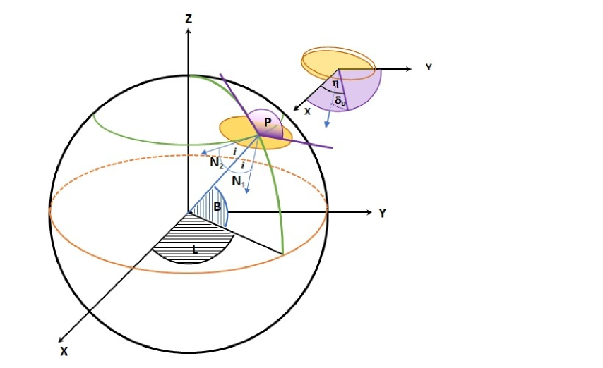


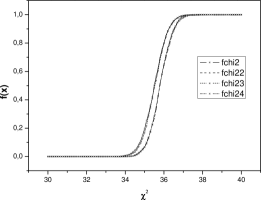

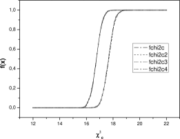

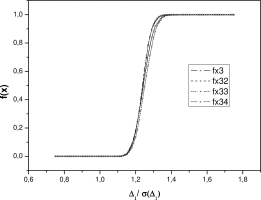
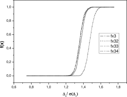
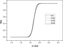


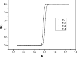


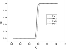
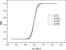

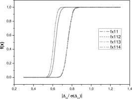

| Test | |||
|---|---|---|---|
| Test | ||||
|---|---|---|---|---|
| angle | ||||
| Test | ||||
|---|---|---|---|---|
| angle | ||||
| Test | ||||
|---|---|---|---|---|
| angle | ||||
| Test | Galaxies | |||||||
|---|---|---|---|---|---|---|---|---|
| Test | ||||||||
| angle | ||||||||
| Test | Galaxies | |||||||
|---|---|---|---|---|---|---|---|---|
| Test | ||||||||
| angle | ||||||||
| Test | Galaxies | |||||||
|---|---|---|---|---|---|---|---|---|
| Test | ||||||||
| angle | ||||||||
| Equatorial coordinates | Supergalactic coordinates | ||||
|---|---|---|---|---|---|
| Sample | Test | ||||
| A | |||||
| — | |||||
| B | |||||
| — | |||||
| Equatorial coordinates | Supergalactic coordinates | ||||
|---|---|---|---|---|---|
| Sample | Test | ||||
| A | |||||
| — | |||||
| B | |||||
| — | |||||
| Sample A | Sample B | |||||
|---|---|---|---|---|---|---|
| Test | ||||||
| BM I | BM I-II | BM II | BM II-III | BM III | ||||||
|---|---|---|---|---|---|---|---|---|---|---|
| Members | 35 | 53 | 59 | 53 | 47 | |||||
| Test | ||||||||||
| BM I | BM I-II | BM II | BM II-III | BM III | ||||||
|---|---|---|---|---|---|---|---|---|---|---|
| Members | 35 | 53 | 59 | 53 | 47 | |||||
| Test | ||||||||||