On-Sky Operations with the ALES Integral Field Spectrograph

Abstract

The integral field spectrograph configuration of the LMIRCam science camera within the Large Binocular Telescope Interferometer (LBTI) facilitates 2 to 5 $\mu$m spectroscopy of directly imaged gas-giant exoplanets. The mode, dubbed ALES, comprises magnification optics, a lenslet array, and direct-vision prisms, all of which are included within filter wheels in LMIRCam. Our observing approach includes manual adjustments to filter wheel positions to optimize alignment, on/off nodding to track sky-background variations, and wavelength calibration using narrow band filters in series with ALES optics. For planets with separations outside our 1”x1” field of view, we use a three-point nod pattern to visit the primary, secondary and sky. To minimize overheads we select the longest exposure times and nod periods given observing conditions, especially sky brightness and variability. Using this strategy we collected several datasets of low-mass companions to nearby stars.

1 INTRODUCTION

At low temperatures gas-giant atmospheres transition from relatively warm, cloudy, and CO-rich (L-types) to relatively cool, and cloud free with CH₄ not CO as the dominant carrier of atmospheric carbon (T-types). This transition is not completely understood especially because it is so abrupt and dramatic. For example, the field brown dwarf population transition beginning at $T_{\mathrm{eff}}$$\sim 1300$ K and ending by $T_{\mathrm{eff}}\sim 1100$ K (e.g., Ref. 1).

The temperature of the L-to-T transition is a function of gravity, with low-gravity objects observed to loft photospheric clouds and maintain atmospheric CO down to much lower temperatures than their higher-gravity counterparts (e.g., Ref. 2). Thus, degeneracies between surface gravity, effective temperature, cloudiness, and chemistry make interpreting spectra of substellar objects challenging. Thermal-infrared (3–5$\mu$m) measurements are essential for breaking these degeneracies because they probe the peak of the emission spectra for cool ($T_{\mathrm{eff}}\lesssim 1000$ K) atmospheres and because they probe the fundamental transitions of the CH₄ and CO molecules. Thus, 3–5 $\mu$m spectral energy distributions are sensitive indicators for understanding carbon chemistry in substellar objects[3].

While essential for a complete understanding of planetary atmospheres, thermal-infrared characterization of exoplanets has received relatively little attention, partly because of the challenging nature of ground-based observations at these wavelengths. The LBTI instrument at the LBT was specifically designed to provide low thermal background for the study of exoplanetary systems [4]. The instrument takes advantage of the observatory’s twin deformable mirror adaptive optics systems to observe at very-high spatial resolution using the minimum number of warm optics.

To facilitate thermal-infrared spectroscopic observations of exoplanets, our team has built the world’s only thermal infrared integral field spectrograph [5]. Integral field spectrographs (IFS) facilitate exoplanet spectroscopy because the techniques of high-contrast imaging can be used to separate planet light from starlight at each wavelength. The instrument, named the Arizona Lenslets for Exoplanet Spectroscopy (ALES), has recently been commissioned and is now producing high-spatial resolution L-band spectra in high-contrast environments.

The ALES IFS was built into the existing LMIRCam module [6] of LBTI. To accomplish this, all the ALES optics, including magnifiers, a lenslet array, and direct-vision prisms, are located within LMIRCam filter wheels. This architecture requires a careful set-up and calibration approach that accommodates the number of moving parts.

In this manuscript, we document our ALES observing strategy which we developed over three semesters while using ALES to observe multiple systems including exoplanets, brown dwarfs and solar system objects. This summer, ALES will undergo a significant upgrade that will improve our usable field of view, spectral resolution, and overall optical quality. New Magnification optics will also make imaging interferometry possible with ALES. (See Hinz et al., and Skemer et al., in these proceedings for more specifics.) After the upgrade, some of the details of our observing strategy may change, but the overall process and general steps of our approach will remain unchanged.

2 Aligning Optics

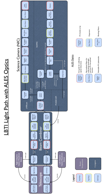
Figure 1: Block diagram of LBTI showing the full ALES light path. All of the ALES optics are inserted by filter wheels, making the design completely modular. We use the NOMIC science camera in parallel with ALES when we implement a three-point nod script to observe widely separated companions. Not shown: four flat mirrors, a ZnSe window between the beam combiner and the science camera, and a fixed pupil stop in the NOMIC light path.

In the following subsections we will refer to elements indicated in Figure 1 in order to describe the set-up and alignment of ALES. In some cases the elements are named different than indicated within the LBTI control software actually used to set up the instrument. In these cases, we list the alternative name in parentheses.

The unique architecture of the LBT telescope, with its two 8.4 diameter mirrors separated by 6.2 meters, facilitates multiple observing modes including co-phased imaging interferometry as well as separated imaging where two images of a target star are made on the detector. In its preliminary configuration ALES is used in single-aperture mode with LBTI as the current magnification optics do not deliver an ALES plate scale that can Nyquist sample the interferometric point spread function (34 milliarcseconds at 3.8 $\mu$m). The ALES field of view is too narrow to make use of dual-sided but spatially separated imaging. An alternative option, overlapped but not co-phased imaging with LBTI, is possible with ALES in principle, but in practice, added operational overheads associated with overlapping the two sides make this mode sub-optimal. A planned ALES upgrade will include new magnification optics that will allow ALES to be used in imaging interferometry mode (Skemer et al., these proceedings).

Single-sided imaging with LBTI/LMIRCam is typically done using a combination of the dual-sided cold stop in LMIRCam Filter Wheel 1 (lmir FW1) and an opaque semi-circle “half moon” in LMIRCam Filter Wheel 2 (lmir FW2). The “half moon” stops the light from the unused side of the telescope in order to reduce the background on the detector. This approach is preferred for most programs requiring only one side with LMIRCam because it is fast to move the “half moon” in and out when switching between programs with different instrument requirements. However, the ALES wavelength calibration filters are also located in Filter Wheel 2 (lmir FW2), so the dual-sided cold stop plus “half moon” approach cannot be used with ALES. Instead, we use a single-sided cold stop in Filter Wheel 1 (lmir FW1). This adds $\sim 5$ mins to the set-up overheads for ALES compared to other single-sided modes, and another $\sim 5$ mins at the end of an ALES observing sequence to replace the dual-sided cold stop for use with other programs.

2.1 Align the Single-Sided Cold Stop

The process for aligning the single-sided cold stop begins by entering pupil-imaging mode. This entails:

• Camera Selector (NIC BEAMDIVT) goes to Trichroic,

• Combined Focal Plane Wheel (NIL NICNAC) goes to 5mm pinhole,

• Filter Wheel 2 (lmir FW2) goes to Open,

• Filter Wheel 2.5 (lmir FW25) goes to Open,

• Filter Wheel 3 (lmir FW3) goes to narrowband 3.9 $\mu$m filter,

• Filter Wheel 4 (lmir FW4) goes to pupil imaging lens.

The next step is to decide which side of the telescope to use. Typically which side is chosen is unimportant, but during intervals of telescope technical difficulties it may be that one side is better suited to ensure stable system performance for science operations. Then the corresponding cold stop, either single-sided left (SXAperture) or single-sided right (DXAperture) should be selected for Filter Wheel 1 (lmir FW1). The position of the stop should be optimized to limit thermal background. Gross vertical alignment is made using small adjustments ( 1000 steps) to Filter Wheel 1 (lmir FW1). Fine adjustments and horizontal adjustments are made using the corresponding right or left side Pupil Alignment Mirrors (roof mirrors). The configured maximum single movement for the roof mirrors is 10,000 steps, and this results in a relatively small motion of the pupil.

2.2 Align the Target with ALES Sweetspot

Once the cold stop is aligned, LMIRCam should be returned to L^′ imaging mode:

• Combined Focal Plane Wheel (NIL NICNAC) goes to Open,

• Filter Wheel 3 (lmir FW3) goes to Open,

• Filter Wheel 4 (lmir FW4) goes to std-L.

The next step is to choose a bright star to facilitate ALES alignment. Stars with m${}_{\mathrm{L}^{\prime}}\lesssim 7$ will allow all alignment steps to be carried out with minimum exposure times. Typically a telluric calibrator or nearby pointing star is used if the science object is fainter than this.

In imaging mode, the image of the target needs to be offset to be coincident with the ALES sweetspot—the portion of the LMIRCam field-of-view that is seen when the ALES magnifier is used. In its current set up the sweet spot is centered on LMIRCam pixel (1388,996). Before offsets can be made, the adaptive-optics loop for the relevant side needs to be locked. After verifying that the AO loop is closed, the required offset in detector coordinates can be calculated using the LMIRCam plate scale, 10.07 milliarcseconds/pixel[7].

The current version of ALES (before an upgrade this summer), suffers from off-axis astigmatism. The best image quality is centered around pixel (900, 1040) in the magnified field of view. To optimize the position of the target, we put in the magnifier and make small telescope offsets, keeping in mind that the magnified field is 180^∘ rotated with respect to the unmagnified image because the refractive magnifier sends the light through focus [5]. To make this step easier, it is helpful to first save a dark image and then subtract it from subsequent frames before displaying on the graphical interface. The process is:

• Filter Wheel 4 (lmir FW4) goes to Blank,

• take an image and use it as a background on the display,

• Filter Wheel 4 (lmir FW4) goes to std-L,

• Magnifier Wheel (Mag Wheel) goes to Refractive Magnifier,

• make small adjustments to the target position with telescope offsets, keeping in mind the field is rotated.

Once the star is positioned as desired, the AO config file should be updated with the corresponding bayside stage positions so that new pointings are acquired with the star at the same location. The offsets should also be “absorbed” by the telescope Pointing Control System so that an absolute (0, 0) offset will return the star to it’s optimal position.

2.3 Align ALES Optics

The ALES configuration includes a magnifier, a lenslet array, a prism and a blocking filter. After following the steps above, the magnifier should already be in place in the Mag Wheel. To complete the set-up we align the lenslet array in the Focal Plane Wheel (lmir APERWHL) and the prism in Filter Wheel 3 (lmir FW3).

First, select the lenslet array in the Focal Plane Wheel (lmir APERWHL). It is important to verify that the lenslet array is properly positioned, meaning that the lenslet spots are parallel to the pixels on the LMIRCam detector. Using a 2-second exposure time is helpful for this step and grabbing a corresponding dark frame for background subtraction in the graphical interface is also helpful. Currently the displayed image in our graphical interface is binned to $512\times 512$ pixels. This can make analyzing the lenslet spots challenging. Our solution is to zoom in on the $512\times 512$ pixel region including the highest optical quality spots. The correct way to zoom is done by selecting the appropriate subframe for the detector and using LMIRCam “slow mode”. In this context, slow-mode does not imply any change in the detector read-out. Rather, the whole $2048\times 2048$ detector is read and saved but only the pixels within the chosen subframe are displayed. This is peculiar to our graphical interface implementation, and allows us to save full ALES frames while viewing full resolution images of a smaller subframe. Once zoomed in, small nudges to the Focal Plane Wheel (lmir APERWHL) can be used to adjust the lenslet array for optical positioning.

Next, the prism and blocking filter should be positioned. Currently ALES has only one spectral mode covering 2.8 through 4.2 $\mu$m at R$\sim 40$. In the future, a wider variety of passbands and spectral resolutions will be available (Skemer et al., these proceedings). Prisms are in Filter Wheel 3 (lmir FW3), and blocking filters are in Filter Wheel 2.5 (lmir FW25). Once positioned the dispersion direction of the spectral traces should be inspected. The optimal dispersion direction results in minimal overlap of neighboring spectra. If spectra appear to collide, the best recourse is to home Filter Wheel 3 (lmir FW3) and then re-select the prism.

In list form the above sequence is:

• Focal Plane Wheel (lmir APERWHL) goes to lenslet array,

• choose $512\times 512$ subframe and set to slow mode,

• Filter Wheel 4 (lmir FW4) goes to Blank,

• save a dark frame for background subtraction,

• Filter Wheel 4 (lmir FW4) goes to Open,

• adjust lenslet array position if needed,

• Filter Wheel 3 (lmir FW3) goes to IFU-prism,

• Filter Wheel 2.5 (lmir FW25) goes to Lspec,

• home and re-position Filter Wheel 3 (lmir FW3) if needed.

Once aligned, it is very important not to touch any of the ALES-specific optics (magnifier, lenslet, prism) before obtaining wavelength calibration frames because the wavelength solution depends on the specific position of all of these elements.

3 Observing

Since LBT is and Alt/Az telescope and the LBTI instrument does not include a derotator, all objects appear to rotate with the parallactic angle on the LMIRCam detector. In closed-loop adaptive optics mode, the AO-guidestar is the axis of rotation. This paradigm requires two ALES observing scenarios, depending on whether or not the object of interest can be seen within the narrow ALES field of view together with the guide star.

3.1 Two-point Nod Sequence

For self-guided targets, including telluric calibrators and solar-system objects (e.g., comets and planetary moons), and for close-in directly imaged exoplanets such as HR 8799 c,d,e (with the primary as the AO-guidestar), we observe with a two-point nod script periodically pointing to the sky in order to track variable background emission. Exposure times for the camera are chosen to be as long as possible without detector saturation. For close-in planets this requirement is relaxed so that pixels covering the core of the stellar PSF are often saturated, though it is important to ensure that pixels at the separation of interest are still linear. With the current LMIRCam set-up, significant non-linearity occurs above 50,000 counts (i.e., ADUs). Typically exposure times are 2 to 3 seconds long. The number of images per nod position is selected so that the telescope is offset every 2 mins.

In order to track and flag highly variable pixels that complicate the extraction and analysis of ALES data, we collect pseudo-dark frames simultaneously with telescope nods. To do this, we spin Filter Wheel 2 (lmir FW2) by 25,000 steps (half a position) and save two or three frames (depending on the exposure time) while the telescope is in motion, thus there are no additional overheads associated with saving these frames.

Exposing science and sky-background frames, nodding, and saving darks while the telescope is in motion are all performed within a script for efficiency. The script coordinates with the adaptive-optics system and begins collecting science and sky data only after AO loops are closed following a telescope move. To facilitate the organization and analysis of ALES data, the script automatically updates the fits headers of each file, setting the FLAG keyword to SCI, DRK, or SKY, for on-source, pseudo-dark, and sky-background frames, respectively.

3.2 Three-point Nod Sequence

Our alternate observing scenario applies to targets more widely separated from their guidestar. This is the case for HR 8799 b, $\kappa$ And b, GJ 504 b, and HD 130948 BC for example. In these cases we must nod the telescope to track rotation of the parallactic angle to ensure that our target of interest remains in the ALES field of view. To achieve this we use a three-point nodding script that alternates pointing at the guide-star, the science target, and a blank sky position to track variable background. Exposure times are selected as above with the added constraint that they should be short enough that the science target does not smear due to rotation within an integration. This typically applies only to the widest separation most quickly rotating objects. We spend two minutes on the science target and two minutes in the sky position for each nod cycle. Since the guide-star is observed only to help anchor our coordinate system we save far fewer frames in this position, usually 4. As in the two-point scenario, our script saves pseudo-darks while the telescope is in motion and automatically updates fits headers for organization. In this case the FLAG keyword is set to PRI, SEC, SKY, or DRK for the guide-star, science target, sky-background, and pseudo-dark frames, respectively.

For our three-point nod script, we use RA and Dec-coordinate absolute (not relative) nods within the script in order to offset to the science position. We use these nod parameters because in this system the guidestar-science object separation vector ($\Delta$RA, $\Delta$Dec) is not a function of time (unlike detector coordinate or relative offsets which change as the field rotates). In this mode, it is particularly important to make sure that any adjustments to the position of the AO-guidestar are ”absorbed” by the telescope pointing control system before executing the script.

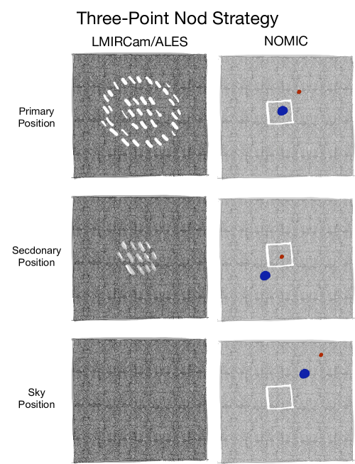
Figure 2: A cartoon illustration of our three-point nod script approach to observing widely separated companions with ALES. The left column represents the sky-subtracted images seen by ALES. The right column represents the field as seen by NOMIC. Using the NOMIC frames we can empirically measure the LBT nods, and use this information to shift and stack faint secondary frames when the secondary is too faint to see in an individual 2-minute nod.

3.2.1 Using NOMIC to Track Nods

We found that imprecise nods prohibited the naive stacking of faint science target data collected with our three-point approach. To circumvent this limitation, we use the NOMIC camera [8] which is positioned within LBTI on the opposite side of a trichroic beam splitter from ALES. The beam splitter sends 1–2.5 $\mu$m and 8–13 $\mu$m light toward NOMIC and 3 to 5 $\mu$m light toward LMIRCam (and ALES). Usually, NOMIC is used as a 10 $\mu$m nulling interferometer, but for our purposes we use it in H-band (1.65 $\mu$m) imaging mode to observe our fields in parallel with ALES. In this way, we can precisely measure the telescope nod-vector using the image of the guidestar on NOMIC, and then use the information to solve for the appropriate image shifts needed to stack our faint-star data. This requires some additional set-up time for three-point nod observations to get NOMIC ready.

First, NOMIC should be put into imaging mode:

• Imaging Dichroic (NIL DICROIC) goes to Imaging,

• Nulling Mirror Slide (NOMIC MSSLIDE) goes to Imaging.

Next, NOMIC should be put into pupil imaging mode:

• NOMIC Filter Wheel 1 (NOMIC FW1) goes to Pupil-imaging-lens,

• NOMIC Filter Wheel 2 (NOMIC FW2) goes to broad N-band (W-10145-9),

• Combined Focal Plane Wheel (NIL NICNAC) goes to 5mm pinhole,

• NOMIC Detector goes to low gain.

Since the Pupil Alignment Mirrors (roof mirrors) are positioned to align the LMIRCam cold stop, we will align the NOMIC cold stop as best we can without touching them:

• NOMIC Pupil Wheel (NOMIC PW) goes to Dual2.54, a double-sided cold stop,

• small adjustments to NOMIC Pupil Wheel (NOMIC PW) move the stop left-right.

NOMIC does not have a single-sided stop like LMIRCam, so to stop light from the side not in use, we send the appropriate Aperture Wheel in the beam combiner to Closed. Lastly, we put NOMIC into H-band imaging mode:

• NOMIC Filter Wheel 1 (NOMIC FW1) goes to Open,

• NOMIC Filter Wheel 2 (NOMIC FW2) goes to H-band (W0164-6),

• Combined Focal Plane Wheel (NIL NICNAC) goes to Open,

• NOMIC Detector goes to High gain.

We adjust the NOMIC exposure time to make sure the guidestar does not saturate, and within our script we set the number of images per nod position such that NOMIC always takes less time gathering images than ALES.

4 Calibrations

To properly interpret ALES images some ALES-specific calibration data is required. These include wavelength calibration frames, lenslet flats, and telluric calibrators.

Wavelength calibration is currently done using a set of four narrow-band photometric filters in series with the ALES optics, upstream of the lenslet array. These R$\sim 100$ filters are unresolved by the ALES prisms and provide single-wavelength spots on the LMIRCam detector. We have have cryogenic traces of our filters and the central wavelengths from short to long are: 2.9, 3.3, 3.5, and 3.9 $\mu$m. For each ALES trace, a second-order polynomial is fit to the position of the four spots to derive the wavelength solution. This approach allows us to identify changes in the wavelength solution as a function of position as the optical quality degrades off axis. Typically $\gtrsim 100$ seconds of exposure time is needed for high S/N in the 2.9 $\mu$m filter, much less is necessary for the 3.9 $\mu$m filter because the background increases dramatically between these two wavelengths.

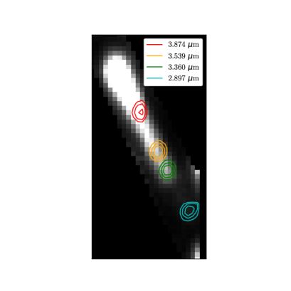
Figure 3: ALES wavelength calibration strategy. Four unresolved narrow-band filters are used in parallel with ALES optics to measure the wavelength solution. A single ALES trace is shown in gray scale. Contours of the narrow-band+ALES images are overlaid.

Since ALES is composed of so many moving parts, it is essential to collect wavelength calibration data before moving any of the ALES optics (to move on to a non-ALES observing program for example). If necessary in a time crunch, observations through the 3.9 $mu$m filter can be made on-sky and then during closed-dome time in the morning a full four-filter set can be collected. In this case, we solve for the rotation and shift necessary to overlap the dome 3.9 $\mu$m frames on top of the sky 3.9 $\mu$m frames. We then apply these corrections to the frames from all four filters before performing the wavelength calibration. This approach is not perfect, since slight mis-alignments of the lenslet array will put a given lens at a different location in the intermediate focal plane, where aberrations are a function of position.

In the future we will have a dedicated wavelength calibration unit for ALES that will include a light-source and monochrometer (Briesemeister et al., these proceedings). In addition to helping wavelength calibrate our data, this unit will facilitate a new spectral extraction mode that will increase our signal to noise and decrease our susceptibility to spaxel crosstalk [9].

A lenslet flat is a flat-field that quantifies the through put of each lenslet in our lenslet array. We do not typically spend time specifically to obtain data for a lenslet flat. Instead, we use the sky-images observed while collecting science data since the background is typically bright enough and very flat across our 1” field of view.

Telluric calibrations for ALES are similar to telluric calibrations for other spectrographs. We typically choose to observe A-type stars to calibrate our 2.8 to 4.2 $\mu$m spectra. In the future, when our Brackett-$\gamma$ mode is implemented, calibrators without strong photospheric hydrogen lines, such as G-type stars, should be selected. In order to not saturate the LMIRCam detector, a calibrator fainter than m${}_{L^{\prime}}\sim 4$ should be chosen. For efficiency a calibrator brighter then m${}_{L^{\prime}}\sim 7$ should be identified. One important and unique requirement for ALES telluric calibration is to make sure that the calibrator overlaps similar spaxels as the science object because the spectral resolution changes with position. Howerver, it is not necessary to get this precise as the resolution is very-low in general and it changes very slowly across the field. For science targets too faint to see in individual frames, it is important to step the calibrator about in the ALES field to ensure that appropriate data is collected.

5 Initial Results

Below we show three example ALES datasets demonstrating our ability to work in the high-contrast environment and to measure spectra of low-mass companions over a variety of separations. In Figure 4 we show the three inner-most directly imaged planets in the HR 8799 system [10]. The image is a sum over the wavelength dimension since the dataset did not include adequate exposure time to attain high signal to noise in each spectral slice. The closest-in planet, separated by $\lesssim 0.4^{\prime\prime}$, is easily separated from the central star, which has been removed using principle component analysis [11, 12] on each spectral slice before stacking. This dataset was collected using the two-point nod script described above and demonstrates our ability to work in the high-contrast environment.

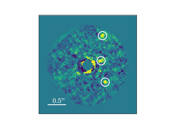
Figure 4: Three planets within $\sim 1^{\prime\prime}$ of the star HR 8799 detected with ALES (highlighted with white circles, Stone et al., in prep). This image shows a sum over the wavelength direction of our ALES spectral cube. The image of the central star has been removed using principle component analysis based angular differential imaging. The inner-most planet is separated by $0.4^{\prime\prime}$ and is 9.5 magnitudes fainter than the primary. These data were collected using a two-point nod sequence.

We also show two datasets obtained using our three-point nod script. In Figure 5 we show the $\kappa$ And system that includes a $\sim 20~{}M_{\mathrm{Jup}}$ companion orbiting a B-type star separated by $1.1^{\prime\prime}$ [13]. We have not made any attempt to remove the image of the star via post-processing, yet the companion is easily visible at high signal-to-noise in each spectral slice owing to the high-strehl and raw-contrast delivered by the LBTI-AO system [14]. In this case, both the star and the companion just fit into the ALES field of view. We used the three-point nod script instead of the two-point nod pattern in order to position the companion where ALES delivers the best optical quality (and highest spectral resolution and minimal spaxel crosstalk).

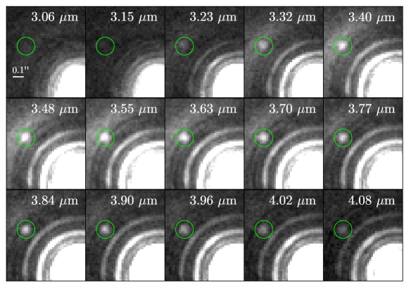
Figure 5: ALES spectral cube of the $\kappa$ And system from Stone et al., in prep. The star is saturated in the lower right corner, and the diffraction pattern expands with wavelength. No attempt to remove the stellar image has been made with these data. The low-mass companion is highlighted with a green circle. These data were taken with a three-point nod pattern to center the companion on the position of the best image quality in the ALES field of view.

In Figure 6 we show an ALES data cube of the brown dwarf binary HD 130948 BC [15]. These two brown dwarfs, separated by $\sim 0.1^{\prime\prime}$, are part of a hierarchical triple system and are in orbit about a main sequence G star separated by $2.6^{\prime\prime}$. ALES facilitates resolved spectroscopy of the brown dwarfs. Since dynamical masses and age constraints exist for this system, these ALES data can be used to ground truth atmospheric models for substellar objects at the wavelengths where JWST will operate. For these observations we used our three-point nod script to observe the brown dwarfs with ALES while guiding the AO using the G star.

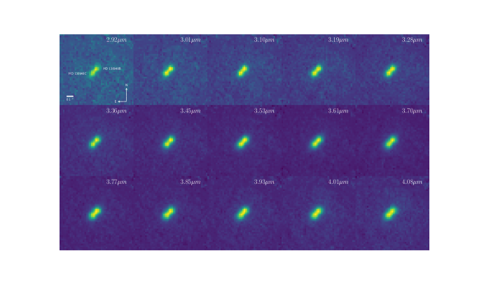
Figure 6: ALES spectral cube of HD130948 BC from Briesemeister et al., in prep. These twin brown dwarfs orbit a main-sequence star as part of a hierarchical triple system. The star, separated by $2.6^{\prime\prime}$, was used as the adaptive optics reference source. These data were taken using our three-point nod script.

- [1] Kirkpatrick, J. D., “New Spectral Types L and T,” Annual Review of Astronomy and Astrophysics 43, 195–245 (Sept. 2005).
- [2] Stephens, D. C., Leggett, S. K., Cushing, M. C., Marley, M. S., Saumon, D., Geballe, T. R., Golimowski, D. A., Fan, X., and Noll, K. S., “The 0.8-14.5 m Spectra of Mid-L to Mid-T Dwarfs: Diagnostics of Effective Temperature, Grain Sedimentation, Gas Transport, and Surface Gravity,” ApJ 702, 154–170 (Sept. 2009).
- [3] Noll, K. S., Geballe, T. R., Leggett, S. K., and Marley, M. S., “The Onset of Methane in L Dwarfs,” ApJ 541, L75–L78 (Oct. 2000).
- [4] Hinz, P. M., Defrère, D., Skemer, A., Bailey, V., Stone, J., Spalding, E., Vaz, A., Pinna, E., Puglisi, A., Esposito, S., Montoya, M., Downey, E., Leisenring, J., Durney, O., Hoffmann, W., Hill, J., Millan-Gabet, R., Mennesson, B., Danchi, W., Morzinski, K., Grenz, P., Skrutskie, M., and Ertel, S., “Overview of LBTI: a multipurpose facility for high spatial resolution observations,” in [Optical and Infrared Interferometry and Imaging V ], 9907, 990704 (Aug. 2016).
- [5] Skemer, A. J., Hinz, P., Montoya, M., Skrutskie, M. F., Leisenring, J., Durney, O., Woodward, C. E., Wilson, J., Nelson, M., Bailey, V., Defrere, D., and Stone, J., “First light with ALES: A 2-5 micron adaptive optics Integral Field Spectrograph for the LBT,” in [Techniques and Instrumentation for Detection of Exoplanets VII ], 9605, 96051D (Sept. 2015).
- [6] Skrutskie, M. F., Jones, T., Hinz, P., Garnavich, P., Wilson, J., Nelson, M., Solheid, E., Durney, O., Hoffmann, W., Vaitheeswaran, V., McMahon, T., Leisenring, J., and Wong, A., “The Large Binocular Telescope mid-infrared camera (LMIRcam): final design and status,” in [Ground-based and Airborne Instrumentation for Astronomy III ], 7735, 77353H (July 2010).
- [7] Maire, A. L., Skemer, A. J., Hinz, P. M., Desidera, S., Esposito, S., Gratton, R., Marzari, F., Skrutskie, M. F., Biller, B. A., Defrère, D., Bailey, V. P., Leisenring, J. M., Apai, D., Bonnefoy, M., Brandner, W., Buenzli, E., Claudi, R. U., Close, L. M., Crepp, J. R., De Rosa, R. J., Eisner, J. A., Fortney, J. J., Henning, T., Hofmann, K. H., Kopytova, T. G., Males, J. R., Mesa, D., Morzinski, K. M., Oza, A., Patience, J., Pinna, E., Rajan, A., Schertl, D., Schlieder, J. E., Su, K. Y. L., Vaz, A., Ward-Duong, K., Weigelt, G., and Woodward, C. E., “The LEECH Exoplanet Imaging Survey. Further constraints on the planet architecture of the HR 8799 system,” A&A 576, A133 (Apr. 2015).
- [8] Hoffmann, W. F., Hinz, P. M., Defrère, D., Leisenring, J. M., Skemer, A. J., Arbo, P. A., Montoya, M., and Mennesson, B., “Operation and performance of the mid-infrared camera, NOMIC, on the Large Binocular Telescope,” in [Ground-based and Airborne Instrumentation for Astronomy V ], 9147, 91471O (July 2014).
- [9] Brandt, T. D., Rizzo, M., Groff, T., Chilcote, J., Greco, J. P., Kasdin, N. J., Limbach, M. A., Galvin, M., Loomis, C., Knapp, G., McElwain, M. W., Jovanovic, N., Currie, T., Mede, K., Tamura, M., Takato, N., and Hayashi, M., “Data reduction pipeline for the CHARIS integral-field spectrograph I: detector readout calibration and data cube extraction,” Journal of Astronomical Telescopes, Instruments, and Systems 3, 048002 (Oct. 2017).
- [10] Marois, C., Zuckerman, B., Konopacky, Q. M., Macintosh, B., and Barman, T., “Images of a fourth planet orbiting HR 8799,” Nature 468, 1080–1083 (Dec. 2010).
- [11] Soummer, R., Pueyo, L., and Larkin, J., “Detection and Characterization of Exoplanets and Disks Using Projections on Karhunen-Loève Eigenimages,” ApJL 755, L28 (Aug. 2012).
- [12] Amara, A. and Quanz, S. P., “PYNPOINT: an image processing package for finding exoplanets,” MNRAS 427, 948–955 (Dec. 2012).
- [13] Carson, J., Thalmann, C., Janson, M., Kozakis, T., Bonnefoy, M., Biller, B., Schlieder, J., Currie, T., McElwain, M., Goto, M., Henning, T., Brandner, W., Feldt, M., Kandori, R., Kuzuhara, M., Stevens, L., Wong, P., Gainey, K., Fukagawa, M., Kuwada, Y., Brandt, T., Kwon, J., Abe, L., Egner, S., Grady, C., Guyon, O., Hashimoto, J., Hayano, Y., Hayashi, M., Hayashi, S., Hodapp, K., Ishii, M., Iye, M., Knapp, G., Kudo, T., Kusakabe, N., Matsuo, T., Miyama, S., Morino, J., Moro-Martin, A., Nishimura, T., Pyo, T., Serabyn, E., Suto, H., Suzuki, R., Takami, M., Takato, N., Terada, H., Tomono, D., Turner, E., Watanabe, M., Wisniewski, J., Yamada, T., Takami, H., Usuda, T., and Tamura, M., “Direct Imaging Discovery of a ”Super-Jupiter” around the Late B-type Star And,” ApJ 763, L32 (Feb. 2013).
- [14] Bailey, V. P., Hinz, P. M., Puglisi, A. T., Esposito, S., Vaitheeswaran, V., Skemer, A. J., Defrère, D., Vaz, A., and Leisenring, J. M., “Large binocular telescope interferometer adaptive optics: on-sky performance and lessons learned,” in [Adaptive Optics Systems IV ], 9148, 914803 (July 2014).
- [15] Potter, D., Martín, E. L., Cushing, M. C., Baudoz, P., Brandner, W., Guyon, O., and Neuhäuser, R., “Hokupa’a-Gemini Discovery of Two Ultracool Companions to the Young Star HD 130948,” ApJ 567, L133–L136 (Mar. 2002).