Belief likelihood function for generalised logistic regression
Abstract
The notion of belief likelihood function of repeated trials is introduced, whenever the uncertainty for individual trials is encoded by a belief measure (a finite random set). This generalises the traditional likelihood function, and provides a natural setting for belief inference from statistical data. Factorisation results are proven for the case in which conjunctive or disjunctive combination are employed, leading to analytical expressions for the lower and upper likelihoods of ‘sharp’ samples in the case of Bernoulli trials, and to the formulation of a generalised logistic regression framework.
1 Introduction
Logistic regression [4] is a popular statistical method for modelling data in which one or more independent observed variables determine an outcome, represented by a binary variable. The framework can also be extended to the multinomial case, and is widely used in various fields, including machine learning, medical diagnosis, and social sciences, to cite a few. Despite its successes, the method has serious limitations. In particular, it has been shown to consistently and sharply underestimate the probability of ‘rare’ events [19]. The term [25] denotes cases in which the training data are of insufficient quality, in the sense that they do not represent well enough the underlying distribution. As a result, scientists are forced to infer probability distributions using information captured in ‘normal’ times (e.g. while a nuclear power plant is working nominally), whereas these distributions are later used to extrapolate results at the ‘tail’ of the curve.
Although corrections to logistic regression have been proposed [19], the root cause of the problem, in our view, our very models of uncertainty are themselves affected by uncertainty: a phenomenon often called ‘Knightian’ uncertainty. The latter can be explicitly modelled by considering convex sets of probability distributions, or ‘credal sets [24, 23]. Random sets [26, 27, 29, 15], in particular, are a sub-class of credal sets induced by probability distributions on the collection of all subsets of the sample space. In the finite case random sets are often called belief functions, a term introduced by Glenn Shafer [28] from a subjective probability perspective.
As we show here, the logistic regression framework can indeed be generalised to the case of belief functions, which themselves generalise classical discrete probability measures. Given a sample space , the traditional likelihood function is equal to the conditional probability of the data given a parameter , i.e., a family of probability distribution functions (PDFs) over parameterised by : , As originally proposed by Shafer and Wasserman [28, 32, 33], belief functions can indeed be built from traditional likelihood functions. However, as we argue here, one can directly define a belief likelihood function, mapping a sample observation to a real number, as a natural set-valued generalisation of the conventional likelihood. It is natural to define such a belief likelihood function as family of belief functions on , , parameterised by . As the latter take values on sets of outcomes, , of which singleton outcomes are mere special cases, they provide a natural setting for computing likelihoods of set-valued observations, in accordance with the random set philosophy.
When applied to samples generated by series of independent trials, under a generalisation of stochastic independence, belief likelihoods factorise into simple products. The resulting lower and upper likelihoods can be easily computed for series of Bernoulli trials, and allows us to formulate a generalised logistic regression framework, in which the mass values of individual trials are constrained to follow a logistic dependence on scalar parameters. The values of the parameters which optimise the lower and upper likelihoods induce a pair of ‘lower’ and ‘upper’ belief functions on the parameter space, whose interval effectively encodes the uncertainty associated with the amount of data at our disposal. Every new observation, possibly in areas of the sample space not previously explored, is mapped to a pair of lower and upper logistic belief functions, which together provide lower and upper estimates for the belief values of each event.
1.1 Contributions
The contributions of the paper are thus as follows:
(1) a belief likelihood function for repeated trials is defined, whenever the uncertainty on individual trials is assumed to be encoded by a belief measure;
(2) elegant factorisation properties are proven for events that are Cartesian products, whenever belief measures are combined by conjunctive rule, leading to the notions of lower and upper likelihoods;
(3) factorisation results are also provided in the case in which the dual, disjunctive combination is used to compute belief and plausibility likelihoods;
(4) analitical expressions of lower and upper likelihoods are provided for the case of Bernoulli trials;
(4) finally, a generalised logistic regression based on lower and upper likelihoods is formulated and analysed, as an alternative inference mechanism to generate belief functions from statistical data.
1.2 Paper outline
After reviewing in Section 2 the logistic regression framework, we recall in Section 3 the necessary notions of the theory of belief functions. In Section 4 the belief likelihood function of repeated trials is defined. In Section 5, the belief likelihood of a series of binary trials is analysed in the conjunctive case. Factorisation results are shown which reduce upper and lower likelihoods of ‘sharp’ samples to products of belief values of individual binary observations, and can be generalised to arbitrary Cartesian products of focal elements. In Section 6 an analysis of the belief likelihood function in the disjunctive case is conducted. General factorisation results holding for series of observations from arbitrary sample spaces are illustrated in Section 7, while analytical expressions for the Bernoulli case are given in Section 8. Finally, a generalised logistic regression framework is outlined (Section 9) in which the masses of the two outcomes are constrained to have a logistic dependency, and dual optimisation problems lead to a pair of lower and upper estimates for the belief measure of the outcomes. Section 10 concludes the paper and points at future work.
2 Logistic regression
Logistic regression allows us, given a sample , where is a binary outcome at time and is the corresponding observed measurement, to learn the parameters of a conditional probability relation between the two, of the form:
| (1) |
where and are two scalar parameters. Given a new observation , (1) delivers the probability of a positive outcome . Logistic regression generalises deterministic linear regression, as it is a function of the linear combination . The trials are assumed independent but not equally distributed, for varies with the time instant of collection. The two scalar parameters in (1) are estimated by maximum likelihood of the sample. After denoting by
| (2) |
the conditional probabilities of the two outcomes, the likelihood of the sample can be expressed as:
where and is a function of . Maximising yields a conditional PDF .
Unfortunately, logistic regression shows clear limitations when the number of samples is insufficient or when there are too few positive outcomes (1s) [19].
Moreover, inference by logistic regression tends to underestimate the probability of a positive outcome [19].
3 Belief functions
3.1 Belief and plausibility measures
Definition 1.
The quantity is called the basic probability number or ‘mass’ [22, 21] assigned to . The elements of the power set associated with non-zero values of are called the focal elements of .
Definition 2.
The belief function (BF) associated with a basic probability assignment is the set function defined as:
| (3) |
The domain on which a belief function is defined is usually interpreted as the set of possible answers to a given problem, exactly one of which is the correct one. For each subset (‘event’) the quantity takes on the meaning of degree of belief that the truth lies in , and represents the total belief committed to a set of possible outcomes by the available evidence .
Another mathematical expression of the evidence generating a belief function is the upper probability or plausibility of an event : , as opposed to its lower probability [6]. The corresponding plausibility function conveys the same information as , and can be expressed as:
3.2 Evidence combination
The issue of combining the belief function representing our current knowledge state with a new one encoding the new evidence is central in belief theory. After an initial proposal by Dempster, several other aggregation operators have been proposed, based on different assumptions on the nature of the sources of evidence to combine.
Definition 3.
The orthogonal sum or Dempster’s combination of two belief functions , defined on the same domain is the unique BF on with as focal elements all the non-empty intersections of focal elements of and , and basic probability assignment:
| (4) |
where denotes the BPA of the input BF , and:
Rather than normalising (as in (4)), Smets’ conjunctive rule leaves the conflicting mass with the empty set:
| (5) |
and is thus applicable to ‘unnormalised’ beliefs [31].
In Dempster’s rule, consensus between two sources is expressed by the intersection of the supported events. When the union is taken to express consensus we obtain the disjunctive rule of combination [20, 34]:
| (6) |
which yields more cautious inferences than conjunctive rules, by producing belief functions that are less ‘committed’, i.e., have larger focal sets. Under disjunctive combination: , input belief values are simply multiplied.
3.3 Conditioning
Belief functions can also be conditioned, rather than combined, whenever we are presented hard evidence of the form ‘ is true’ [3, 12, 18, 14, 9, 35, 17].
In particular, Dempster’s combination naturally induces a conditioning operator. Given a conditioning event , the ‘logical’ (or ‘categorical’, in Smets’ terminology) belief function such that is combined via Dempster’s rule with the a-priori belief function . The resulting BF is the conditional belief function given a la Dempster, denoted by .
3.4 Multivariate analysis
In many applications, we need to express uncertain information about a number of distinct variables (e.g., and ) taking values in different domains ( and , respectively). The reasoning process needs then to take place in the Cartesian product of the domains associated with each individual variable.
Let then and be two sample spaces associated with two distinct variables, and let be a mass function on . The latter can be expressed in the coarser domain by transferring each mass to the projection of on . We obtain a marginal mass function on , denoted by:
Conversely, a mass function on can be expressed in by transferring each mass to the cylindrical extension of . The vacuous extension of onto will then be:
| (7) |
The associated BF is denoted by .
4 Belief likelihood of repeated trials
Let , for be a parameterised family of belief functions on , the space of quantities that can be observed at time , depending on a parameter . A series of repeated trials then assumes values in , whose elements are tuples of the form . We call such tuples ‘sharp’ samples, as opposed to arbitrary subsets of the space of trials. Note that we are not assuming the trials to be equally distributed at this stage, nor we assume that they come from the same sample space.
Definition 4.
The belief likelihood function of a series of repeated trials is defined as:
| (8) |
where is the vacuous extension (7) of to the Cartesian product where the observed tuples live, and is an arbitrary combination rule.
In particular, when the subset reduces to a sharp sample, , we can define the following generalisations of the notion of likelihood.
Definition 5.
We call the quantities
| (9) |
lower likelihood and upper likelihood, respectively, of .
5 Binary trials: the conjunctive case
Belief likelihoods factorise into simple products, whenever conjuctive combination is employed (as a generalisation of classical stochastic independence) in Definition 4, and trials with binary outcomes are considered.
5.1 Focal elements of the belief likelihood
Let us first analyse the case . We seek the Dempster’s sum , where .
Figure 1 is a diagram of all the intersections of focal elements of the two input BF on .
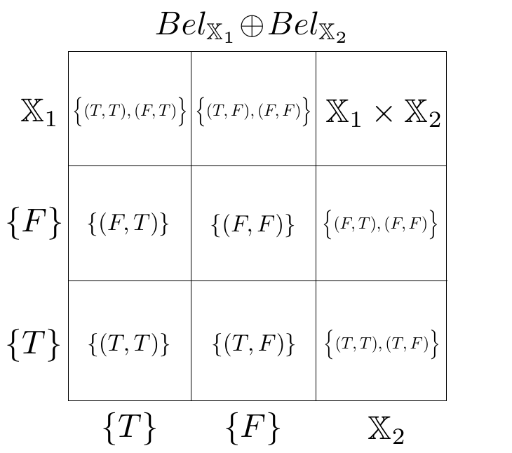
There are distinct, non-empty intersections, which correspond to the focal elements of . According to Equation (4), the mass of focal element , , , is then:
| (10) |
Note that the result holds when using the conjunctive rule as well (5), for none of the intersections is empty, hence no normalisation is required. Nothing is assumed about the mass assignment of and .
We can now prove the following Lemma.
Lemma 1.
For any the belief function , where , has focal elements, namely all possible Cartesian products of non-empty subsets of , with BPA:
Proof.
The proof is by induction. The thesis was shown to be true for in Equation (10). In the induction step, we assume that the thesis is true for , and prove it for . If , defined on , has as focal elements the -products with for all , its vacuous extension to will have as focal elements the -products of the form: , with for all .
The belief function is defined on , with three focal elements: , and . Its vacuous extension to thus has the following three focal elements:
,
and
.
When computing on the common refinement we need to compute the intersection of their focal elements, namely:
for all , . All such intersections are distinct for distinct focal elements of the two belief functions to combine, and there are no empty intersection. By Dempster’s rule (4) their mass is equal to the product of the original masses, i.e.:
Since we assumed that the factorisation holds for , the thesis easily follows. ∎
As no normalisation is involved in the combination , Dempster’s rule coincides with the conjunctive rule and Lemma 1 holds for as well.
5.2 Factorisation for ‘sharp’ tuples
The following becomes then a simple corollary.
Theorem 1.
When using either or as a combination rule in the definition of belief likelihood function, the following decomposition holds for tuples , , which are the singletons elements of , with :
| (11) |
Proof.
There is evidence to support the following as well.
Conjecture 1.
When using either $\scriptstyle{\cap}$⃝ or as a combination rule in the definition of belief likelihood function, the following decomposition holds for the associated plausibility values on tuples , , which are the singletons elements of , with :
| (12) |
Indeed we can write:
| (13) |
By Lemma 1 all the subsets with non-zero mass are Cartesian products of the form , . We then need understand the nature of the focal elements of which are subsets of an arbitrary singleton complement .
For binary spaces , by definition of Cartesian product, each such is obtained by replacing a number of components of the tuple with a different subset of (either or ). There are such sets of components in a list of . Of these components, in general will be replaced by , while the other will be replaced by . Note that not all components can be replaced by , since the resulting focal element would contain the tuple .
The following argument can be proved for , under the additional assumption that are equally distributed with , and .
If this is the case, for fixed values of and all the resulting focal elements have the same mass value, namely: , where , and . As there are exactly such focal elements, (13) can be written as:
which can be rewritten as:
A change of variable , where when , when , allows us to write it as:
since , . Now, as
we obtain: By Newton’s binomial, the latter is equal to since . Again, by Newton’s binomial, we get:
5.3 Factorisation for Cartesian products
Decomposition (11) is equivalent to what Smets calls conditional conjunctive independence [30]. In fact, for binary spaces factorisation (11) generalises to all subsets of samples which are Cartesian products of subsets of , respectively: , for all .
Corollary 1.
Whenever , , under conjunctive combination we have that:
| (14) |
Proof.
As by Lemma 1 all the focal elements of are Cartesian products of the form , , it follows that is equal to:
But since if for some the resulting Cartesian product would not be a subset of . Thus,
| (15) |
For all ’s, that are singletons of , necessarily and we can write (15) as:
If the frames are binary, , those ’s that are not singletons coincide with , so that we have:
The quantity is, according to the definition of conjunctive combination, the sum of the masses of all the possible intersections of (cylindrical extensions of) focal elements of , , thus they add up to 1. In conclusion (forgetting the conditioning on in the derivation for sake of readability): and we have (14). ∎
Corollary 1 states that conditional conjunctive independence always holds for events that are Cartesian products, whenever the involved frames are binary.
6 Binary trials: the disjunctive case
Similar factorisation results hold when using the (more cautious) disjunctive combination .
6.1 Structure of the focal elements
As in the conjunctive case, we first analyse the case . We seek the disjunctive combination , where each has as focal elements , and . Figure 2 is a diagram of all the unions of focal elements of the two input BFs on their common refinement .
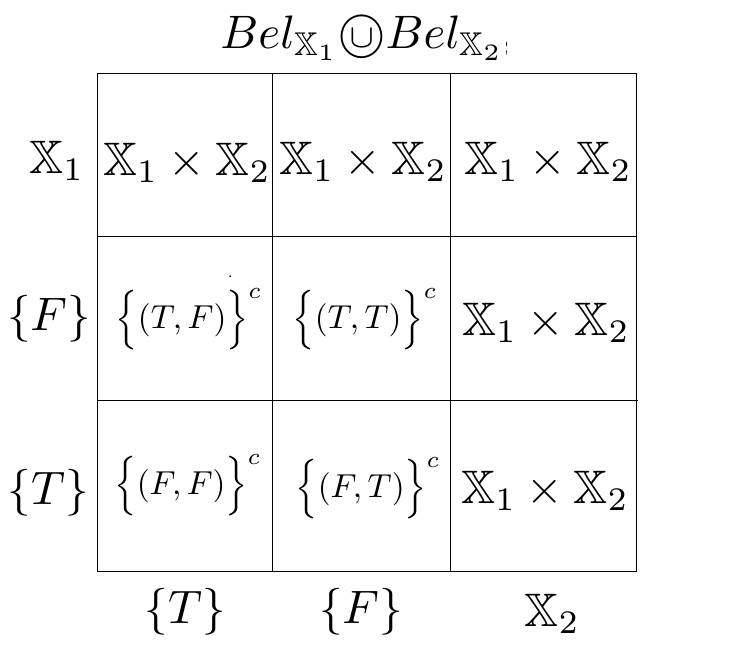
There are distinct such unions, the focal elements of , with masses:
We can now prove the following Lemma.
Lemma 2.
The belief function , where , has focal elements, namely all the complements of the -tuples of singleton elements , with BPA:
| (16) |
plus the Cartesian product itself, with mass value given by normalisation.
Proof.
The proof is by induction. The case was proven above. In the induction step, we assume that the thesis is true for , namely that the focal elements of have the form:
| (17) |
where . We need to prove it true for .
The vacuous extension of (17) has trivially the form:
Note that only singletons of are not in , for any given tuple .
The vacuous extension to of a focal element of is instead:
Now, all the elements of , except for , are also elements of . Hence, the union reduces to the union of and . The only singleton element of not in is therefore , , for it is neither in nor in . All such unions are distinct. Thus, by definition of , their mass is which by inductive hypothesis is equal to (16). Unions involving either or are equal to by the property of the union operator. ∎
6.2 Factorisation
Theorem 2.
In the hypotheses of Lemma 2, when using disjunctive combination $\scriptstyle{\cup}$⃝ in the definition of belief likelihood function, the following decomposition holds:
| (18) |
Proof.
Note that for all tuples , as the set has non-empty intersection with all the focal elements of .
7 General factorisation results
The argument of Lemma 1 is in fact valid for the conjunctive combination of belief functions defined on an arbitrary collection of finite spaces.
Theorem 3.
For any the belief function , where are finite spaces, has as focal elements all the Cartesian products of focal elements , with BPA:
The proof is similar to that of Lemma 1, and is omitted for lack of space. It follows that:
Corollary 2.
When using either $\scriptstyle{\cap}$⃝ or as a combination rule in the definition of belief likelihood function, the following decomposition holds for tuples , , which are the singletons elements of , with any finite frames of discernment:
| (19) |
8 Lower and upper likelihoods of Bernoulli trials
In the case of Bernoulli trials, where not only there is a single binary sample space, and conditional independence holds, but the random variables are assumed equally distributed, the conventional likelihood reads as , where , is the number of successes () and the total number of trials.
Let us then compute the lower likelihood function for a series of Bernoulli trials, under the assumption that all the BFs , , coincide (the analogous of equidistribution), with parameterised by , (where, this time, ).
Corollary 3.
Under the above assumptions, the lower and upper likelihoods of the sample are:
| (20) |
The above decomposition for , in particular, is valid under the assumption that Conjecture 1 holds, at least for Bernoulli trials, as the evidence seems to suggest.
After normalisation, these can be seen as probability distribution functions (PDFs) over the (belief) space of all belief functions definable on [5, 7, 8].
Having observes a series of trials, , , one may then seek the belief function on which best describes the observed sample, i.e., the optimal values of the two parameters and .
 |
|
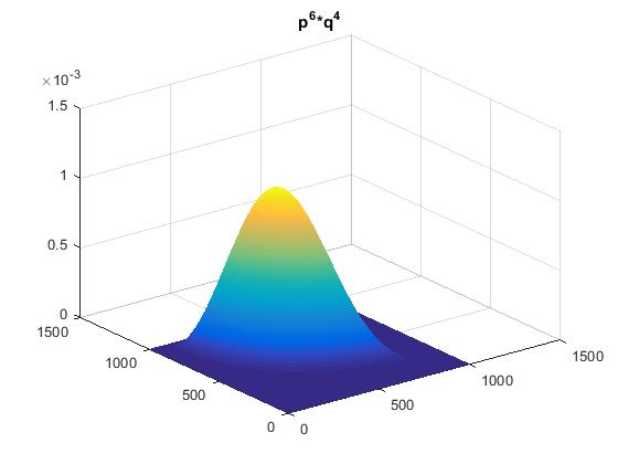
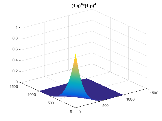
Figure 3 plots the both lower and upper likelihoods (20) for the case of successes over trials.
Both subsume the traditional likelihood , as their section for , although this is particularly visible for the lower likelihood (top). In particular, the maximum of the lower likelihood is the traditional ML estimate , .
This makes sense, for the lower likelihood is highest for the most committed belief functions (i.e., for probability measures).
The upper likelihood (bottom) has a unique maximum in : this is the vacuous belief function on , with .
The interval of belief functions joining with is the set of belief functions such that , i.e., those which preserve the ratio between the observed empirical counts.
9 Generalising logistic regression
Based on Theorem 1 and Conjecture 1,
we can also generalise logistic regression (Section 2) to a belief function setting by replacing the conditional probability on with a belief function (, , ) on .
Note that, just as in a traditional logistic regression setting (Section 2), the belief functions associated with different input values are not equally distributed.
After writing , the lower and upper likelihoods can be expressed as:
The question becomes how to generalise the logit link between observations and outputs , in order to seek an analytical mapping between observations and belief functions over a binary frame. Just assuming:
| (21) |
as in the classical contraint (2), does not yield any analytical dependency for . To address this issue we can, for instance, add a parameter such that the following relationship holds:
| (22) |
We can then seek lower and upper optimal estimates for the parameter vector :
| (23) |
Plugging these optimal parameters into (21), (22) will then yield a lower and an upper family of conditional belief functions given (i.e., an interval of belief functions):
Given any new test observation , this generalised logistic regression method will then output a pair of lower and upper belief functions on , as opposed to a sharp probability value as in the classical framework. As each belief function itself provides a lower and an upper probability for each event, both the lower and the upper regressed BFs will provide an interval for the probability of success, whose width will reflect the uncertainty encoded by the training set of sample series.
9.1 Optimisation
The problems (23) are both constrained optimisation ones (contrarily to the classical case, where and the optimisation problem is unconstrained).
Indeed, the parameter vector must be such that:
Fortunately the number of constraints can be reduced by noticing that, if and have the analytical forms (21) and (22), respectively, then for all whenever .
The objective function can also be simplified by taking the logarithm. In the lower likelihood case we get111Derivations are omitted due to lack of space.:
We then need to analyse the Karush-Kuhn-Tucker (KKT) necessary conditions for the optimality of the solution of a nonlinear optimisation problem
subject to differentiable constraints: .
If is a local optimum, under some regularity conditions then there exist constants , , called KKT multipliers, such that the following conditions hold:
-
1.
(Stationarity);
-
2.
Primal feasibility: for all ;
-
3.
Dual feasibility: for all ;
-
4.
Complementary slackness: for all .
In our case the constraints are:
, and the Lagrangian becomes:
The stationarity conditions thus read as , i.e.:
| (24) |
where, as usual, is as in (21).
Complementary slackness reads instead as follows:
| (25) |
Standard gradient descent methods can be applied to the above systems of equations to get the optimal parameters of our generalised logistic regressor. Similar calculations hold for the upper likelihood problem. A multi-objective optimisation setting in which the lower likelihood is minimised as the upper likelihood is maximised can be envisaged, to generate the most cautious interval of estimates.
10 Conclusions
In this paper, stimulated by the inability of logistic regression to encode uncertainty induced by scarcity of samples in certain areas of the sample space, and inference mechanisms for belief measures which take the classical likelihood function at face value, we defined a belief likelihood function for repeated trials, as an inference methodology both more in line with the random set philosophy of inherently set-valued observations, and capable of allowing a promising generalisation of logistic regression. We analysed the factorisation properties of the belief likelihood function when either conjunctive or disjunctive combination is applied, in particular for the case of binary spaces, and computed the lower and upper likelihoods of series of Bernoulli trials. Eventually, we proposed a generalised logistic regression framework which leads to a pair of dual constrained optimisation problems, which can be solved by standard methods.
A number of interesting research lines lie ahead. Among others, a systematic comparison with other approaches to belief function inference, or the computation of belief and plausibility likelihood for other major combination rules. As far as generalised logistic regression is concerned, different parameterisations of the belief functions involved need to be explored. A comprehensive testing of the robustness of the generalised framework in standard estimation problems, including rare event analysis, needs to be conducted to validate this new procedure. The method, unlike traditional ones, can naturally cope with missing data (represented by vacuous observations ), therefore providing a robust framework for logistic regression which can deal with incomplete series of observations.
References
- [1] T. Augustin, Modeling weak information with generalized basic probability assignments, Data Analysis and Information Systems - Statistical and Conceptual Approaches Springer, 1996, pp. 101–113.
- [2] C. A. Bail, Lost in a random forest: Using big data to study rare events, Big Data & Society 2(2), 2015.
- [3] A. Chateauneuf and J.Y. Jaffray, Some characterization of lower probabilities and other monotone capacities through the use of Moebius inversion, Math. Soc. Sci. 17 (1989), 263–283.
- [4] D. R. Cox, The Regression Analysis of Binary Sequences, Journal of the Royal Statistical Society. Series B 20 (1958), no. 2, 215–242.
- [5] F. Cuzzolin, A geometric approach to the theory of evidence, IEEE Transactions on Systems, Man and Cybernetics part C 38(4), 522–534, 2008.
- [6] F. Cuzzolin, Three alternative combinatorial formulations of the theory of evidence, Intelligent Data Analysis 14 (2010), no. 4, 439–464.
- [7] F. Cuzzolin, Visions of a generalized probability theory, Lambert Academic Publishing, 2014.
- [8] F. Cuzzolin, The geometry of uncertainty, Springer-Verlag, 2018.
- [9] D. Denneberg, Conditioning (updating) non-additive probabilities, AOR 52, 21–42, 1994.
- [10] D. Denneberg and M. Grabisch, Interaction transform of set functions over a finite set, Information Sciences 121, 149–170, 1999.
- [11] D. Dubois & H. Prade, A set theoretical view of belief functions, Int. J. Intelligent Systems 12, 193–226, 1986.
- [12] R. Fagin and J.Y. Halpern, A new approach to updating beliefs, Proc. of UAI, 1991, pp. 347–374.
- [13] A. Gelman, N. Silver, and A. Edlin, What is the probability your vote will make a difference?, Economic Inquiry 50(2), 321–326, 2012.
- [14] I. Gilboa & D. Schmeidler, Updating ambiguous beliefs, J. of Economic Theory 59 (1993), 33–49.
- [15] H. T. Hestir, H. T. Nguyen, and G. S. Rogers, A random set formalism for evidential reasoning, Conditional Logic in Expert Systems, North Holland, 1991, pp. 309–344.
- [16] Y. T. Hsia, Characterizing belief functions with minimal commitment, Proceedings of IJCAI-91, 1991, pp. 1184–1189.
- [17] M. Itoh and T. Inagaki, A new conditioning rule for belief updating in the Dempster-Shafer theory of evidence, Transactions of the Society of Instrument and Control Engineers 31(12), 2011–17, 1995.
- [18] J. Y. Jaffray, Bayesian updating and belief functions, IEEE Tr. SMC 22 (1992), 1144–1152.
- [19] G. King and L. Zeng, Logistic regression in rare events data, Political Analysis 9 (2001), 137–163.
- [20] I. Kramosil, Probabilistic analysis of belief functions, Springer, 2001.
- [21] R. Kruse, D. Nauck, and F. Klawonn, Reasoning with mass, Proc. of UAI, 1991, pp. 182–187.
- [22] R. Kruse, E. Schwecke, and F. Klawonn, On a tool for reasoning with mass distribution, Proc. of IJCAI, vol. 2, 1991, pp. 1190–1195.
- [23] H. Kyburg, Bayesian and non-Bayesian evidential updating, AIJ 31(3), 271–294, 1987.
- [24] I. Levi, The enterprise of knowledge, 1980.
- [25] J. Husler M. Falk and R-D. Reiss, Laws of small numbers: Extremes and rare events, 2004.
- [26] G. Matheron, Random sets and integral geometry, John Wiley & Sons, 1974.
- [27] H. T. Nguyen, On random sets and belief functions, J. Math. Anal. Appl. 65 (1978), 531–542.
- [28] G. Shafer, A mathematical theory of evidence, Princeton University Press, 1976.
- [29] G. Shafer, P. P. Shenoy, and K. Mellouli, Propagating belief functions in qualitative Markov trees, IJAR 1(4), 349–400,1987.
- [30] Ph. Smets, Belief functions : The disjunctive rule of combination and the generalized Bayesian theorem, IJAR 9, 1–35, 1993.
- [31] Ph. Smets, The nature of the unnormalized beliefs encountered in the transferable belief model, Proc. of UAI, 1992, pp. 292–29.
- [32] L. Wasserman, Some applications of belief functions to statistical inference, PhD thesis, 1987.
- [33] , Belief functions and statistical inference, Canadian Journal of Statistics 18, 183–196, 1990.
- [34] Koichi Yamada, A new combination of evidence based on compromise, Fuzzy Sets and Systems 159(13), 1689 – 1708, 2008.
- [35] C. Yu and F. Arasta, On conditional belief functions, IJAR 10, 155–172, 1994.