Asynchronous Variance-reduced Block Schemes for Composite Nonconvex Stochastic Optimization: Block-specific Steplengths and Adapted Batch-sizes

Abstract

This work considers the minimization of a sum of an expectation-valued coordinate-wise $L_{i}$-smooth nonconvex function and a nonsmooth block-separable convex regularizer where $i$ denotes the block index. We propose an asynchronous variance-reduced algorithm, where in each iteration, a single block is randomly chosen to update its estimates by a proximal variable sample-size stochastic gradient scheme, while the remaining blocks are kept invariant. Notably, each block employs a steplength that is in accordance with its block-specific Lipschitz constant while block-specific batch-sizes are random variables updated at a rate that grows either at a geometric or a polynomial rate with the (random) number of times that block is selected. We show that every limit point for almost every sample path is a stationary point and establish the ergodic non-asymptotic rate of $\mathcal{O}(1/K)$ in terms of expected sub-optimality. Iteration and oracle complexity to obtain an $\epsilon$-stationary point are shown to be $\mathcal{O}(1/\epsilon)$ and $\mathcal{O}(1/\epsilon^{2})$, respectively. Furthermore, under a $\mu$-proximal Polyak-Łojasiewicz condition with the batch size increasing at a geometric rate, we prove that the suboptimality diminishes at a geometric rate, the optimal deterministic rate while iteration and oracle complexity to obtain an $\epsilon$-optimal solution are proven to be $\mathcal{O}((L_{\rm max}/\mu)\ln(1/\epsilon))$ and $\mathcal{O}\left((L_{\rm ave}/\mu)(1/\epsilon)^{1+c}\right)$, respectively where $L_{\max}$ and $L_{ave}$ denote the maximum and average of the block-specific Lipschitz constants and $c\geq 0$. In the single block setting, we obtain the optimal oracle complexity $\mathcal{O}(1/\epsilon)$. In pursuit of less aggressive sampling rates, when the batch sizes increase at a polynomial rate, we show that the suboptimality decays at a corresponding polynomial rate and establish the iteration and oracle complexity as well. Finally, preliminary numerics support our theoretical findings, displaying significant improvements over schemes where steplengths are based on global Lipschitz constants.

1 Introduction

In this paper, we consider the following composite stochastic programming:

$$\vspace{-0.1in}\min_{x\in\mathbb{R}^{d}}\ F(x)\triangleq\bar{f}(x)+\sum_{i=1}^{n}r_{i}(x_{i}),$$ (1)

where $x_{i}\in\mathbb{R}^{d_{i}}$, $x\in\mathbb{R}^{d}$ is partitioned into $n$ blocks as $x=(x_{1},\cdots,x_{n})$ with $d\triangleq\sum_{i=1}^{n}d_{i}$, $r_{i}:\mathbb{R}^{d_{i}}\to\mathbb{R}$ is a convex nonsmooth function, $\bar{f}(x)\triangleq\mathbb{E}_{\xi}[f(x_{1},\cdots,x_{n},\xi)]$ is an expectation-valued smooth possibly nonconvex function with coordinate-wise $L_{i}$-Lipschitz continuous gradients, the random vector $\xi:{\Omega}\to\mathbb{R}^{m}$ is defined on the probability space $({\Omega},{\cal F},\mathbb{P})$, and $f:\mathbb{R}^{d}\times\mathbb{R}^{m}\to\mathbb{R}$ is a scalar-valued function. Suppose that problem (1) has at least one solution. Let $X^{*}$ and $F^{*}$ denote the set of optimal solutions and the optimal function value, respectively. Nonsmoothness may be addressed through the proximal operator [34, 25], defined as

$$\textrm{prox}_{\alpha r}(x)\ \triangleq\ \mathop{\rm argmin}_{y}\left(r(y)+{1\over 2\alpha}\|y-x\|^{2}\right),$$ (2)

where $r(\cdot)$ is a closed and convex function, $\alpha>0,$ and the argmin is uniquely defined. We will propose an asynchronous proximal variance-reduced block scheme for solving the problem (1).

1.1 Prior research.

We first review the literature on proximal, variance-reduced, and block methods.

(i) Proximal-gradient methods. Proximal-gradient methods and their accelerated variants are among the most important methods for solving composite convex problem $f(x)+r(x)$ (also see forward-backward splitting (FBS) methods [21, 6, 22]). While accelerated (or unaccelerated) schemes [2] display non-asymptotic convergence rates in function value of $\mathcal{O}(1/k^{2})$ (or $(\mathcal{O}(1/k))$), FBS methods [4, 38] display linear convergence when $\nabla f(x)$ is strongly monotone. Nonconvex extensions have been studied in [1, 12, 17], where the convergence to a stationary point is shown in [1] while rate statements are provided under both the Kurdyka-Łojasiewicz (KL) property [12] and the Polyak-Łojasiewicz (PL) condition [17] (where a linear rate is proven).

(ii) Variance-reduced schemes. A stochastic proximal gradient method was presented in [35] for solving composite convex stochastic optimization, where the a.s. convergence and a mean-squared convergence rate $\mathcal{O}(1/k)$ were developed in strongly convex regimes, in sharp contrast with the linear rate of convergence in deterministic settings. Variance reduction and variable sample-size schemes have gained increasing relevance in first-order methods for stochastic convex optimization [36, 15, 13, 14, 16]; in the class of variable sample-size schemes, the true gradient is replaced by the average of an increasing batch of sampled gradients, progressively reducing the variance of the sample-average. In strongly convex regimes, linear rates were shown for stochastic gradient methods [36, 16] and extragradient methods [15], while for merely convex optimization problems, accelerated rates of $\mathcal{O}(1/k^{2})$ and $\mathcal{O}(1/k)$ were proven for smooth [13, 16] and nonsmooth [15] regimes, respectively. Mini-batch stochastic approximation methods were developed in [14] for nonconvex stochastic composite optimization. Alternative variance reduction schemes like SAGA and SVRG, applied to finite-sum machine learning problems [29, 30, 42, 31], rely on periodic use of the exact gradient, leading to recovery of deterministic convergence rates. For example, geometric rates were provided by [31] for proximal SAGA and SVRG algorithms in nonconvex regimes under the proximal PL inequality. The variance reduced schemes have been widely applied to the data-driven applications, e.g., the phase retrieval problem [41, 40] that aims at reconstructing a general signal vector from magnitude-only measurements.

(iii) Block coordinate descent (BCD) schemes. BCD methods [10] have been widely used in machine learning and optimization, where variables are partitioned into manageable blocks and in each iteration, a single block is chosen to update while the remaining blocks remain fixed. Recently, in [26], coordinate-friendly operators were investigated that perform low-cost coordinate updates and it is shown that a variety of problems in machine learning can be efficiently resolved by such an update. The convergence properties of cyclic BCD methods has been extensively analyzed in [39, 28, 43]. Nesterov considered a randomized BCD method [23] and proved sublinear and linear convergence in terms of expected objective value for general convex and strongly convex cases, respectively. In [32], proximal (but unaccelerated) extensions were developed to contend with composite problems (also see [32, 9, 43, 45, 47]), while in [11], an accelerated proximal RBCD scheme was presented with a rate of $\mathcal{O}(1/k^{2}).$ In more recent work [7], diverse block selection rules are considered and linear statements are provided for deterministic nonconvex problems under the PL condition.

1.2 Motivations.

We consider a class of techniques that combine variance reduced and block-based schemes for solving the nonconvex nonsmooth stochastic programs, drawing inspiration from two seminal papers. Of these, the first by Xu and Yin [44] proposes a block stochastic gradient (BSG) method that cyclically updates blocks of variables. The second paper, by Dang and Lan [8], presents a stochastic block mirror-descent scheme reliant on randomly choosing and updating a single block by a mirror-descent stochastic approximation method. In [44] and [8], rates are provided in the convex setting while in nonconvex regimes, Dang and Lan [8] present non-asymptotic rates. Yet, there are several shortcomings that motivate the present research: (1) Centralized batch sizes. The schemes in  [44, 8] require a centrally specified batch-size across all blocks requiring global knowledge of the global clock, i.e. iteration $k$; (2) Shorter steps. Block-invariant steplengths utilize the global Lipschitz constant leading to significantly shorter steps and poorer performance; (3) No almost sure convergence guarantees. Almost sure convergence guarantees are unavailable for BCD schemes for general nonconvex problems; (4) Sub-optimal rate statements. Optimal deterministic rates via variance-reduced schemes are unavailable but have been alluded to in convex regimes [44, Rem. 7]; Refinements via the PL condition remain open questions.

SC,C,NC: Strongly convex, convex, nonconvex; p-PL: proximal P-L, $\delta\geq 0$
App. Metric Asym/Rate/complexity Comments [44] NC – $\mathbb{E}[d(0,\partial F(x(k))]\to 0$ C $\mathbb{E}[F(x(k))-F^{*}]$ $\mathcal{O}(1/\sqrt{k})$ (i) Centralized batch-size $N_{k}$; (ii) Central. step depend. on global $L$; (iii) No rate for nonconvex; SC $\mathbb{E}[\|x(k)-x^{*}\|^{2}]$ $\mathcal{O}(1/k)$ (iv) sub-linear rates for SC [8] NC $\mathbb{E}[\|G_{\alpha}(x_{\alpha,K})\|^{2}]$ rate: $\mathcal{O}(1/K)$ iteration: $\mathcal{O}\left(nL_{\max}/\epsilon\right)$ oracle: $\mathcal{O}\left(n^{2}\nu^{2}L_{\max}/\epsilon^{2}\right)$ (i) Centralized batch-size $N_{k}$ ; (ii) Central stepsize depend on $L_{\max}$; (iii) Inferior constants dependent on $L_{\rm\max}$; C $\mathbb{E}[F(\bar{x}_{K})-F^{*}]$ $\mathcal{O}(1/\sqrt{K})$, $\mathcal{O}(1/K)$ (SC) This work NC – a.s. conv. to stationary points (i) a.s. convergence (unavailable in [44, 8]) $\mathbb{E}[\|G_{\alpha}(x_{\alpha,K})\|^{2}]$ rate: $\mathcal{O}(1/K)$ iteration: $\mathcal{O}\left(nL_{\rm ave}/\epsilon\right)$ oracle: $\mathcal{O}\left(n^{2}\nu^{2}L_{\rm ave}/\epsilon^{2}\right)$ (ii) Block-specific stepsize depend on $L_{i}$ $\implies$ better empirical behavior; (iii) Optimal rates depend. on $L_{\rm ave}$ (Rather than $L$, $L_{\max}$ [44, 8]) p-PL $\mathbb{E}[F(x(k))-F^{*}]$ geometric batch-size: geometric rate iteration: $\mathcal{O}\left({nL_{\max}\over\mu}\ln(1/\epsilon)\right)$ oracle: $\mathcal{O}\Big{(}{nL_{\rm ave}\over\mu}(1/\epsilon)^{1+\delta}\Big{)}$ (iv) Block-specific random. batch-sizes $\implies$ no central coordination of clocks (v) Optimal geometric rate under p-PL poly. batch-size: deg. $v$: polynomial rate $\mathcal{O}(k^{-v})$ iteration: $\mathcal{O}((1/\epsilon)^{1/v})$ oracle: $\mathcal{O}\left((1/\epsilon)^{1+1/v}\right)$

Table 1: List of literature on block-structured stochastic optimization

1.3 Summary of Contributions.

We address the aforementioned gaps through designing a novel algorithm that combines a randomized BCD method with a proximal VSSG method, reliant on block-specific steplengths based on locally available $L_{i}$ without knowledge of the central Lipschitz constant, leading to larger steplengths and improved behavior, and on random block-specific batch-sizes (adapted to its block-selection history) without knowledge of the global clock, leading to lower informational coordination requirements. We make the following contributions supported by numerics in Section 5. Table 1 formalizes the distinctions in our scheme, while Table 2 compares our results with deterministic rates for nonconvex regimes.

(a) Iteration complexity in smooth case $(r(x)=0)$
block selection rule PL general nonconvex unif. deterministic [7] $\mathcal{O}\left({nL_{\max}\over\mu}\ln\left({F(x_{1})-F^{*}\over\epsilon}\right)\right)$ $\mathcal{O}\left({nL_{\max}\left(F(x(0))-F^{*}\right)\over\epsilon}\right)$ stoch. (This work) $\mathcal{O}\left({nL_{\max}\over\mu}\ln\left({F(x_{1})-F^{*}\over\epsilon}+{n\nu^{2}\over\epsilon}\right)\right)$ $\mathcal{O}\left({nL_{\max}\left(F(x(0))-F^{*}\right)\over\epsilon}\right)$ non-unif. deterministic [7] $\mathcal{O}\left({nL_{\rm ave}\over\mu}\ln\left({F(x_{1})-F^{*}\over\epsilon}\right)\right)$ $\mathcal{O}\left({nL_{\rm ave}\left(F(x(0))-F^{*}\right)\over\epsilon}\right)$ stoch. (This work) $\mathcal{O}\left({nL_{\rm ave}\over\mu}\ln\left({F(x_{1})-F^{*}\over\epsilon}+{n\nu^{2}\over\epsilon}\right)\right)$ $\mathcal{O}\left({nL_{\rm ave}\left(F(x(0))-F^{*}\right)\over\epsilon}\right)$ (b) Iteration complexity in nonsmooth case $(r(x)\neq 0)$
block selection rule PL general nonconvex unif. deterministic[7] $\mathcal{O}\left({nL_{\max}\over\mu}\ln\left({F(x_{1})-F^{*}\over\epsilon}\right)\right)$ $\mathcal{O}\left({nL_{\max}\left(F(x(0))-F^{*}\right)\over\epsilon}\right)$ stoch. (This work) $\mathcal{O}\left({nL_{\max}\over\mu}\ln\left({F(x_{1})-F^{*}\over\epsilon}+{n\nu^{2}\over\epsilon}\right)\right)$ $\mathcal{O}\left({nL_{\max}\left(F(x(0))-F^{*}\right)\over\epsilon}\right)$

Table 2: Comparison with deterministic rates for nonconvex block methods

(I) In Section 3, we prove that every limit point for almost every sample path is a stationary point under appropriately chosen batch sizes and show that the ergodic mean-squared error of the gradient mapping diminishes at a rate $\mathcal{O}(1/K)$. We then establish that for any given $\epsilon>0,$ the iteration complexity (no. of proximal evaluations) and oracle complexity (no. of sampled gradients) to obtain an $\epsilon$-stationary point are $\mathcal{O}(nL_{\max}/\epsilon)$ and $\mathcal{O}(n^{2}{\color[rgb]{0,0,0}\sigma}^{2}L_{\max}^{2}L_{\min}^{-1}\epsilon^{-2})$ with uniform block selection, where $L_{\max}\triangleq\max_{i}L_{i}$, $L_{\min}\triangleq\min_{i}L_{i}$, and $\sigma^{2}$ denotes a uniform bound on the variance of gradient noise. When the blocks are chosen as per a non-uniform distribution with probabilities $L_{i}\left(\sum_{i=1}^{n}L_{i}\right)^{-1}$ for each $i=1,\cdots,n$, the iteration and oracle complexity are improved to $\mathcal{O}(nL_{\rm ave}/\epsilon)$ and $\mathcal{O}(n^{2}{\color[rgb]{0,0,0}\sigma}^{2}L_{\rm ave}/\epsilon^{2})$ with $L_{\rm ave}\triangleq\sum_{i=1}^{n}L_{i}/n$. This represents a constant factor improvement in the rate from $L_{\max}$ (in [8]) to $L_{\rm ave}$. Preliminary numerics reveal that block-specific steplengths lead to significant improvements in empirical behavior (see Table 5). In addition, we show that if the batch-sizes increase at a quadratic rate with the number of times a particular block is chosen, the choice of batch-size sequences no longer relies on the knowledge of global Lipschitzian information.

(II) In Section 4, we consider a class of nonconvex functions satisfying the proximal PL condition with parameter $\mu$ (see Assumption 3) and prove that when the block-specific batch size is random and increases at a suitable geometric rate with the number of times the block is selected, the expectation-valued optimality gap diminishes at a geometric rate. In addition, with uniform block selection, the iteration and oracle complexity to obtain an $\epsilon$-optimal solution are $\mathcal{O}\left({(nL_{\max}/\mu)}\ln(1/\epsilon)\right)$ and $\mathcal{O}\Big{(}{nL_{\rm ave}\over\mu}(1/\epsilon)^{\big{(}1+{1\over n\kappa_{\min}-1}\big{)}{L_{\max}\over L_{\min}}}\Big{)}$ respectively, where $\kappa_{\min}\triangleq L_{\min}/\mu$. While in the smooth regimes with a non-uniform block selection, the iteration and oracle complexity bounds are improved to $\mathcal{O}\left({nL_{\rm ave}\over\mu}\ln\left({1\over\epsilon}\right)\right)$ and $\mathcal{O}\Big{(}{nL_{\rm ave}\over\mu}(1/\epsilon)^{\big{(}1+{1\over n\kappa_{\min}-1}\big{)}{L_{\rm ave}\over L_{\min}}}\Big{)}$, respectively. Specifically, when $n=1$, the optimal oracle complexity $\mathcal{O}\left({L\over\mu\epsilon}\right)$ is obtained. Notably, these rates match the deterministic versions in [7]. We further show that when the batch size increases at a polynomial rate of degree $v\geq 1$, the convergence rate is $\mathcal{O}(k^{-v})$ and the corresponding iteration and oracle complexity are respectively $\mathcal{O}(v(1/\epsilon)^{1/v})$ and $\mathcal{O}\left(e^{v}v^{2v+1}(1/\epsilon)^{1+1/v}\right)$.

2 Asynchronous Block Proximal Stochastic Gradient Algorithm

We assume access to a proximal oracle (PO) that outputs $\textrm{prox}_{\alpha r_{i}}(x_{i})$ at any point $x_{i}\in\mathbb{R}^{d_{i}}$ for any $\alpha>0.$ Since the exact gradient $\nabla\bar{f}(x)$ is unavailable in a closed form, we assume there exists a stochastic first-order oracle (SFO) such that for every $i\in\mathcal{N}\triangleq\{1,\cdots,n\}$ and for any given $x,\xi$, a sampled gradient $\nabla_{x_{i}}f(x,\xi)$ is returned, which is an unbiased estimator of $\nabla_{x_{i}}\bar{f}(x)$. We aim to develop efficient algorithms for obtaining an $\epsilon$-optimal solution, where the efficiency is measured by the iteration complexity (no. of PO calls) and the oracle complexity (no. of SFO calls). Time is slotted at $k=0,1,2,\dots$. Block $i$ at time $k$ holds a state $x_{i}(k)\in\mathbb{R}^{d_{i}}$ that is an estimate for the corresponding coordinates of the optimal solution. We propose an asynchronous variance-reduced block stochastic gradient scheme (Algorithm 1) where at time instant $k,$ a block $i\in\mathcal{N}$ is randomly chosen with probability $p_{i}$ to compute the proxima update (3), where $\alpha_{i}$ is the constant steplength and $N_{i}(k)$ is the number of sampled gradients utilized at block $i$, respectively. To be specific, the steplength $\alpha_{i}$ depends on its block-specific Lipschitz constant $L_{i}$ and the batch-size $N_{i}(k)$ is a function of the random number of times block $i$ is selected up to time $k.$ We will specify the selections of $\alpha_{i}$ and $N_{i}(k)$ upon the performance analysis in Sections 3 and 4.

Algorithm 1 Asynchronous variance-reduced block stochastic gradient algorithm

Let $k:=0$, $x_{i}(0)\in\mathbb{R}^{d_{i}}$ and $0<p_{i}<1$ for $i=1,\ldots,n$ such that $\sum_{i=1}^{n}p_{i}=1.$

1. Pick $i_{k}=i\in\mathcal{N}$ with probability $p_{i}$.

2. If $i_{k}=i$, then block $i$ updates its state $x_{i}(k+1)$ as follows:

   $$x_{i}(k+1)=\textrm{prox}_{\alpha_{i}r_{i}}\left(x_{i}(k)-\alpha_{i}{\sum_{j=1}^{N_{i}(k)}\nabla_{x_{i}}f(x(k),\xi_{j}(k))\over N_{i}(k)}\right),$$ (3)

   where $\alpha_{i}>0$ is the steplength of block $i$, $N_{i}(k)$ is the number of sampled gradients utilized at block $i$, and samples $\{\xi_{j}(k)\}_{j=1}^{N_{i}(k)}$ are randomly generated from the probability space $({\Omega},{\cal F},\mathbb{P})$. Otherwise, $x_{j}(k+1):=x_{j}(k)$ if $j\neq i_{k}$.

3. If $k>K$, stop and return $\{x(k)\}_{k=0}^{K}$; Else, $k:=k+1$ and return to (S.1).

Remark 1

In fact, Algorithm 1 does not require a global coordinator to coordinate the block selection. The block selection rule (S.1.) accommodates the Poisson model employed by [3] as a special case, where each block $i$ is activated according to a local Poisson clock that ticks according to a Poisson process with rate $\varrho_{i}>0$. Suppose that the local Poisson clocks are independent and there is a virtual global clock which ticks whenever any of the local Poisson clocks tick, then the global clock ticks according to a Poisson process with rate $\sum_{i=1}^{n}\varrho_{i}$. Let $Z_{k}$ denote the time of the $k$-th tick of the global clock. Since the local Poisson clocks are independent, with probability one, there is a single block whose Poisson clock ticks at time $Z_{k}$ with probability $\mathbb{P}(i_{k}=i)={\varrho_{i}\over\sum_{i=1}^{n}\varrho_{i}}\triangleq p_{i}.$ In addition, note by (S.2.) and the algorithmic parameter selection rule that each block $i$ maintains a local clock counting the number of its block updates, and that the update (3) does not necessitate knowledge of either the global Lipschitz constant or the virtual global clock. As such, Algorithm 1 is an asynchronous scheme with limited coordination across blocks. Thus, in practical applications, Algorithm 1 might be helpful for the decentralized implementations compared to those designed in [8] and [44].

If the observation noise $w_{i}(k)$ of the exact gradient is defined as

$$w_{i}(k+1)\triangleq\tfrac{\sum_{j=1}^{N_{i}(k)}\nabla_{x_{i}}f(x(k),\xi_{j}(k){\color[rgb]{0,0,0})}}{N_{i}(k)}-\nabla_{x_{i}}\bar{f}(x(k)),$$ (4)

then (3) may be rewritten as

$$x_{i}(k+1)=\textrm{prox}_{\alpha_{i}r_{i}}\big{(}x_{i}(k)-\alpha_{i}\left(\nabla_{x_{i}}\bar{f}(x(k))+w_{i}(k+1)\right)\big{)}.$$ (5)

By taking $r_{i}(x_{i})$ as an indicator function of a convex set $X_{i}$, i.e., $r_{i}(x_{i})=0$ if $x_{i}\in X_{i}$ and $r_{i}(x_{i})=+\infty$ otherwise, then the problem (1) reduces to the stochastic programming $\min_{x_{i}\in X_{i},i\in\mathcal{N}}\mathbb{E}\left[f(x_{1},\cdots,x_{n},\xi)\right].$ In this case, the update (3) reduces to the variable sample-size projected stochastic gradient method:

$$x_{i}(k+1)=\mathbf{P}_{X_{i}}\left(x_{i}(k)-\alpha_{i}\left(\nabla_{x_{i}}\bar{f}(x(k))+w_{i}(k+1)\right)\right),$$

where $\mathbf{P}_{X_{i}}(x_{i})$ denotes the projection of $x_{i}$ onto the set $X_{i}.$ This can be thought as a generalization of the schemes proposed in [36, 15] for solving constrained stochastic convex program.

We denote the $\sigma$-field of the entire information used by Algorithm 1 up to (and including) the update of $x(k)$ by $\mathcal{F}_{k}.$ Then $N_{i}(k)$ is adapted to $\mathcal{F}_{k}$ when $N_{i}(k)$ is a function of the random number of times block $i$ is selected up to time $k.$ We impose the following conditions on the objective functions and observation noises.

Assumption 1

(i) $r_{i}$ is a proper lower semicontinuous and convex function with effective domain $\mathcal{R}_{i}$ required to be compact. (ii) There exists a constant $L_{i}>0$ such that for any $x_{i}^{\prime}\in\mathcal{R}_{i}$ and any $x\in\Pi_{j=1}^{n}\mathcal{R}_{j}$, $\|\nabla_{x_{i}}\bar{f}(x)-\nabla_{x_{i}}\bar{f}(x_{1},\dots,x_{i-1},x_{i}^{\prime},x_{i+1},\dots,x_{n})\|\leq L_{i}\|x_{i}-x_{i}^{\prime}\|.$

Assumption 2

(i) There exists $\sigma>0$ such that for any $i\in\mathcal{N}$ and all $k\geq 1$, $\mathbb{E}[\|w_{i}(k+1)\|^{2}|\mathcal{F}_{k}]\leq{{\color[rgb]{0,0,0}\sigma^{2}}\over N_{i}(k)}~{}a.s.$; (ii) $i_{k}$ is independent of $\mathcal{F}_{k}$ for all $k\geq 1.$

Remark 2

Assumption 1(i) requires the effective domain of each block’s nonsmooth convex regularizer to be a compact set. For example, if $r_{i}(x_{i})$ is set to be an indicator function of a convex set $X_{i}$, then it is required that $X_{i}$ be a compact set. Such a condition guarantees that the iterate sequence $\{x(k)\}$ produced by Algorithm 1 is uniformly bounded. Assumption 1(ii) necessitates the gradient of the nonconvex smooth term $\bar{f}(x)$ to be block-wise Lipschitz continuous. Assumption 2(i) can be satisfied if the sampled gradients are independently generated and $\mathbb{E}[\|\nabla_{x_{i}}f(x,\xi)-\nabla_{x_{i}}\bar{f}(x)\|^{2}]$, the variance of the stochastic gradient noise, is uniformly bounded.

3 Convergence to Stationary Points

In this section, we will prove the almost sure convergence of iterates to a stationary point and establish the non-asymptotic rate of Algorithm 1.

3.1 Preliminary Lemmas

Before presenting the convergence results, we recall a preliminary result from [31, Lemma 2].

Lemma 1

Suppose $y\triangleq\textrm{prox}_{\alpha r}(x-\alpha g)$ for some $g\in\mathbb{R}^{d}.$ Then for any $z\in\mathbb{R}^{d},$

$$\bar{f}(y)+r(y) \leq\bar{f}(z)+r(z)+(y-z)^{T}(\nabla\bar{f}(x)-g)+\left(\frac{L}{2}-{1\over 2\alpha}\right)\|y-x\|^{2}$$

$$+\left(\frac{L}{2}+{1\over 2\alpha}\right)\|z-x\|^{2}-{1\over 2\alpha}\|y-z\|^{2}.$$

We now give a simple relation on the conditional expectation of the function value in the following lemma, for which the proof can be found in Appendix A. This is an important preliminary result because the convergence results to be presented are essentially obtained through a recursive application of this basic lemma.

Lemma 2

Suppose that Assumptions 1 and 2(ii) hold. Let $\{x(k)\}$ be generated by Algorithm 1, where $0<\alpha_{i}\leq{1\over L_{i}}$ for each $i=1,\cdots,n$. Define

$$\bar{x}_{i}(k+1)\triangleq\textrm{prox}_{\alpha_{i}r_{i}}\left(x_{i}(k)-\alpha_{i}\nabla_{x_{i}}\bar{f}(x(k))\right)$$ (6)

as the update if the true gradient is used. Then the following recursion holds almost surely (a.s.):

$$\begin{split}\mathbb{E}\big{[}F(x(k+1))|\mathcal{F}_{k}\big{]}&\leq F(x(k))-\sum_{i=1}^{n}p_{i}\left({1\over 2\alpha_{i}}-L_{i}\right)\|\bar{x}_{i}(k+1)-x_{i}(k)\|^{2}\\ &+{1\over 2}\mathbb{E}\left[\alpha_{i_{k}}\|w_{i_{k}}(k+1)||^{2}|\mathcal{F}_{k}\right],\quad\forall k\geq 1.\end{split}$$ (7)

Throughout the paper, all inequalities and equalities between random variables are assumed to hold a.s., but we often omit to write “a.s.” for simplicity.

3.2 Asymptotic Convergence

From Assumption 1(i) it is seen that the sequence of estimates $\{x(k)\}$ produced Algorithm 1 is bounded. We now establish the almost sure convergence by showing that for every limit point of almost every sample path $\{x(k)\}$ is a stationary point of problem (1).

Theorem 1

Let $\{x(k)\}$ be generated by Algorithm 1. Suppose Assumptions 1 and 2 hold, and that for each $i=1,\cdots,n$, $0<\alpha_{i}<{1\over 2L_{i}}$ and $\sum_{k=0}^{\infty}{1\over N_{i}(k)}<\infty~{}a.s.$ . Then every cluster point of almost every sample path $\{x(k)\}$ is a stationary point.

Proof. Note by Assumption 2(i) that

$$\mathbb{E}\left[\alpha_{i_{k}}\|w_{i_{k}}(k+1)||^{2}|\mathcal{F}_{k}\right]\leq\sum_{i=1}^{n}\mathbb{E}\left[\alpha_{i}\|w_{i}(k+1)||^{2}|\mathcal{F}_{k}\right]\leq\sum_{i=1}^{n}{\alpha_{i}\sigma^{2}\over N_{i}(k)}.$$

Note that ${1\over 2\alpha_{i}}-L_{i}>0$ by $0<\alpha_{i}<{1\over 2L_{i}}$. Then by recalling that $\sum_{k=0}^{\infty}{1\over N_{i}(k)}<\infty~{}a.s.$, we may then apply [33, Thm. 1] to inequality (7) and conclude that $F(x(k))$ converges almost surely and $\sum\limits_{k=1}^{\infty}\sum_{i=1}^{n}p_{i}\left({1\over 2\alpha_{i}}-L_{i}\right)\|\bar{x}_{i}(k+1)-x_{i}(k)\|^{2}<\infty~{}a.s.$ . This implies that

$$\sum\limits_{k=0}^{\infty}\|\bar{x}(k+1)-x(k)\|^{2}<\infty,~{}a.s.$$ (8)

Then for almost every sample path, we have that $\|\bar{x}(k+1)-x(k)\|\to 0$ as $k\to\infty.$ Let $\hat{x}$ be a cluster point of any such sequence $\{x(k)\}$. Then there exists a subsequence $\{x(k_{t})\}$ such that $\lim\limits_{t\to\infty}x(k_{t})=\hat{x}$ and hence $\lim\limits_{t\to\infty}\bar{x}(k_{t}+1)=\hat{x}$ by (8). For any $i=1,\cdots,n$, using the definitions (2) and (6), we obtain that

$$\bar{x}_{i}(k+1)=\mathop{\rm argmin}_{y\in\mathbb{R}^{d_{i}}}\Big{[}\nabla_{x_{i}}\bar{f}(x(k))^{T}(y-x_{i}(k))+{1\over 2\alpha_{i}}\|y-x_{i}(k)\|^{2}+r_{i}(y)\Big{]}.$$ (9)

Then by using the first-order optimality condition, we obtain for all $t:$

$$-{1\over\alpha_{i}}\left(\bar{x}_{i}(k_{{t}}+1)-{x_{i}(k_{t})}\right)\in\nabla_{x_{i}}\bar{f}\left({x(k_{t})}\right)+\partial r_{i}\left({\bar{x}_{i}(k_{t}+1)}\right).$$ (10)

By passing to the limit in (10), using $\|\bar{x}(k_{t}+1)-x(k_{t})\|\to 0~{}a.s.,$ by $\lim\limits_{t\to\infty}{x(k_{t})}=\lim\limits_{t\to\infty}{\bar{x}(k_{t}+1)}={\hat{x}}$, and the continuity of $\nabla_{x_{i}}\bar{f}{(\cdot)}$ and the closedness of $\partial r_{i}$, we obtain that $0\in\nabla_{x_{i}}\bar{f}(\hat{x})+\partial r_{i}(\hat{x}_{i})$ for each $i=1\dots,n.$ Thus, $0\in\nabla\bar{f}(\hat{x})+\partial r(\hat{x}),$ implying that $\hat{x}$ is a stationary point of (1). $\Box$

Remark 3

(i) For any $i\in\mathcal{N}$ and $k\geq 1$, define $\Gamma_{i}(k)\triangleq\sum_{p=0}^{k-1}I_{[i_{p}=i]}$ as the number of updates block $i$ has carried out up to time $k$, where $I_{[a=b]}=1$ if $a=b$, and $I_{[a=b]}=0$ otherwise. Thus, $\Gamma_{i}(k)$ is adapted to $\mathcal{F}_{k}$, and $\sum_{k=0}^{\infty}{1\over N_{i}(k)}<\infty$ holds almost surely by setting $N_{i}(k)\triangleq\lceil(\Gamma_{i}(k)+1)^{1+\delta}\rceil$ for some $\delta>0$. From [18, Lemma 7], it follows that for almost every $\omega\in\Omega$, there exists a sufficiently large $\tilde{k}$ possibly contingent on the sample path $\omega$ such that for any $k\geq\tilde{k},$ $\Gamma_{i}(k)\geq{kp_{i}\over 2},i=1,\cdots,n.$

(ii) If $\bar{f}(x)$ is convex, then Theorem 1 implies that $F(x(k))$ converges almost surely to the optimal function value $F^{*}$, and every cluster point of almost every sample path $\{x(k)\}$ is a global minimum to the problem (1).

3.3 Non-asymptotic Rate

Recall that for convex optimization, a frequently-used metric is the sub-optimality metric $F(x)-F^{*}$ or the distance to the optimal solution set $d(x,X^{*})$. However, in nonconvex optimization, the iterates might converge to stationary points that are not necessarily global minima, and as a consequence, the standard metric cannot be applied. Thus, one crucial problem in analyzing Algorithm 1 for nonconvex problems lies in the selection of the convergence criterion. In smooth regimes, it is typical to use $\|\nabla\bar{f}(x)\|$ while in nonsmooth settings, an appropriate alternative is the proximal gradient mapping [31]: $G_{\alpha}(x)={1\over\alpha}\Big{(}x-\textrm{prox}_{\alpha r}\big{(}x-\alpha\nabla\bar{f}(x)\big{)}\Big{)}$. Then $x^{0}\in\mathbb{R}^{d}$ satisfying $G_{\alpha}(x^{0})=0$ is a stationary point of (1). We now analyze the rate of convergence of Algorithm 1, and establish iteration and oracle complexity bounds to obtain an $\epsilon$-stationary point, by using the following metric to measure stationarity.

$$G_{i,\alpha_{i}}(x)={\frac{x_{i}-{\rm prox}_{\alpha_{i}r_{i}}\left(x_{i}-\alpha_{i}\nabla_{x_{i}}\bar{f}(x)\right)}{\alpha_{i}}},~{}\forall i\in\mathcal{N},~{}\mathbf{G}_{\bm{\alpha}}(x)\triangleq\left(G_{i,\alpha_{i}}(x)\right)_{i=1}^{n}.$$ (11)

It is seen that any zero of $\mathbf{G}_{\bm{\alpha}}(x)$ is a stationary point of (1). Next, we establish a result for Algorithm 1 when the block is chosen according to a uniform distribution.

Theorem 2

Suppose Assumptions 1 and 2 hold. Let $\{x(k)\}$ be generated by Algorithm 1, where $p_{i}={1\over n}$ and $\alpha_{i}={1\over 4L_{i}}$ for each $i=1,\cdots,n$. Let $x_{\alpha,K}$ be chosen from $\{x(k)\}_{k=0}^{K}$ as per a uniform distribution. We have the following bound on the mean-squared error:

$$\mathbb{E}\left[\|\mathbf{G}_{\bm{\alpha}}(x_{\alpha,K})\|^{2}\right]\leq{16nL_{\max}\left(\mathbb{E}[F(x(0))]-F^{*}\right)\over K+1}+{2\sigma^{2}L_{\max}\over K+1}\sum_{i=1}^{n}\sum_{k=0}^{K}L_{i}^{-1}\mathbb{E}[N_{i}(k)^{-1}].$$ (12)

Then for any given $\epsilon>0,$ by setting $K=\bar{K}_{1}(\epsilon)\triangleq{32nL_{\max}\left(\mathbb{E}[F(x(0))]-F^{*}\right)\over\epsilon}$ and $N_{i}(k)\equiv\bar{N}_{1}(\epsilon)\triangleq{4n\sigma^{2}L_{\max}\over\epsilon L_{\min}},$ the iteration and oracle complexity to obtain an $\epsilon$-stationary point such that $\mathbb{E}\left[\|\mathbf{G}_{\bm{\alpha}}(x_{\alpha,K})\|^{2}\right]\leq\epsilon$ are $\bar{K}_{1}(\epsilon)$ and $\bar{K}_{1}(\epsilon)\bar{N}_{1}(\epsilon)$, respectively.

Proof. Note by $\mathbb{P}(i_{k}=i)=p_{i}$ and Assumption 2(i), we obtain that

$$\mathbb{E}\left[\alpha_{i_{k}}\|w_{i_{k}}(k+1)||^{2}\right]=\sum_{i=1}^{n}p_{i}\alpha_{i}\mathbb{E}\left[\|w_{i}(k+1)||^{2}\right]\leq\sum_{i=1}^{n}{\alpha_{i}p_{i}\sigma^{2}}\mathbb{E}\left[N_{i}(k)^{-1}\right].$$

By taking unconditional expectations of (7) and rearranging the terms, the following holds.

$$\begin{split}&\mathbb{E}\left[\sum_{i=1}^{n}p_{i}\left({1\over 2\alpha_{i}}-L_{i}\right)\|\bar{x}_{i}(k+1)-x_{i}(k)\|^{2}\right]\\ &\leq\mathbb{E}\big{[}F(x(k))\big{]}-\mathbb{E}\big{[}F(x(k+1))\big{]}+{1\over 2}\sum_{i=1}^{n}{\alpha_{i}p_{i}\sigma^{2}}\mathbb{E}\left[N_{i}(k)^{-1}\right].\end{split}$$ (13)

Thus, by summing up (13) from $k=0$ to $K$, we have that

$$\begin{split}&\sum_{k=0}^{K}\mathbb{E}\left[\sum_{i=1}^{n}p_{i}\left({1\over 2\alpha_{i}}-L_{i}\right)\|\bar{x}_{i}(k+1)-x_{i}(k)\|^{2}\right]\\ &\leq\mathbb{E}[F(x(0))]-\mathbb{E}\left[F(x(K+1))\right]+{\sigma^{2}\over 2}\sum_{k=0}^{K}\sum_{i=1}^{n}\alpha_{i}p_{i}\mathbb{E}\left[N_{i}(k)^{-1}\right].\end{split}$$ (14)

By the definitions (6) and (11), $\alpha_{i}={1\over 4L_{i}}$,and $p_{i}={1\over n}$, we have that

$$p_{i}\left({1\over 2\alpha_{i}}-L_{i}\right)\|\bar{x}_{i}(k+1)-x_{i}(k)\|^{2}=p_{i}\alpha_{i}\left({1\over 2}-\alpha_{i}L_{i}\right)\left({\|\bar{x}_{i}(k+1)-x_{i}(k)\|\over\alpha_{i}}\right)^{2}$$

$$={1\over 16nL_{i}}\left\|G_{i,\alpha_{i}}(x(k))\right\|^{2}\geq{1\over 16nL_{\max}}\left\|G_{i,\alpha_{i}}(x(k))\right\|^{2}.$$

This combined with (14), $F(x_{K+1})\geq F^{*}$, and $p_{i}={1\over n}$ implies that

$${1\over 16nL_{\max}}\sum_{k=0}^{K}\mathbb{E}\left[\|\mathbf{G}_{\bm{\alpha}}(x(k))\|^{2}\right]\leq\mathbb{E}[F(x(0))]-F^{*}+{\sigma^{2}\over 8n}\sum_{i=1}^{n}{1\over L_{i}}\sum_{k=0}^{K}\mathbb{E}\left[N_{i}(k)^{-1}\right].$$

Therefore, by multiplying both sides of the above equation by ${16nL_{\max}\over K+1}$, by using

$$\mathbb{E}\left[\|\mathbf{G}_{\bm{\alpha}}(x_{\alpha,K})\|^{2}\right]={1\over K+1}\sum_{k=0}^{K}\mathbb{E}\left[\|\mathbf{G}_{\bm{\alpha}}(x(k))\|^{2}\right]$$

we obtain (12). Since $N_{i}(k)=\bar{N}_{1}(\epsilon)$, we have ${1\over K+1}\sum_{k=0}^{K}\mathbb{E}\left[N_{i}(k)^{-1}\right]={1\over\bar{N}_{1}(\epsilon)}.$ This combined with (12) produces the following bound.

$$\begin{split}\mathbb{E}\left[\|\mathbf{G}_{\bm{\alpha}}(x_{\alpha,K})\|^{2}\right]\leq{16nL_{\max}\left(\mathbb{E}[F(x(0))]-F^{*}\right)\over\bar{K}_{1}(\epsilon)+1}+{2n\sigma^{2}L_{\max}\over\bar{N}_{1}(\epsilon)L_{\min}}\leq\epsilon.\end{split}$$ (15)

Since a single block is chosen to be updated at each iteration, the total number of samples used to update $x(K)$ is $\sum_{k=0}^{K-1}\sum_{i=1}^{n}N_{i}(k)I_{[i_{k}=i]}=\bar{K}_{1}(\epsilon)\bar{N}_{1}(\epsilon).$ Then the number of PO and SFO calls required to ensure that $\mathbb{E}\left[\|\mathbf{G}_{\bm{\alpha}}(x_{\alpha,K})\|^{2}\right]\leq\epsilon$ are $\bar{K}_{1}(\epsilon)$ and $\bar{K}_{1}(\epsilon)\bar{N}_{1}(\epsilon)$, respectively. $\Box$

In the following, we analyze the rate of convergence of Algorithm 1 with the active block chosen via a non-uniform distribution constructed using block-specific Lipschitz constants.

Theorem 3

Suppose Assumptions 1 and 2 hold. Let $\{x(k)\}$ be generated by Algorithm 1, where $p_{i}={L_{i}\over\sum_{i=1}^{n}L_{i}}$ and $\alpha_{i}={1\over 4L_{i}}$ for each $i=1,\ldots,n$. Then

$$\mathbb{E}\left[\|\mathbf{G}_{\bm{\alpha}}(x_{\alpha,K})\|^{2}\right]\leq{16nL_{\rm ave}\left(\mathbb{E}[F(x(0))]-F^{*}\right)\over K+1}+{2\sigma^{2}\over K+1}\sum_{i=1}^{n}\sum_{k=0}^{K}\mathbb{E}\left[N_{i}(k)^{-1}\right].$$ (16)

Thus, for any given $\epsilon>0,$ by setting $K=\bar{K}_{2}(\epsilon)={32nL_{\rm ave}\left(\mathbb{E}[F(x(0))]-F^{*}\right)\over\epsilon}$ and $N_{i}(k)\equiv\bar{N}_{2}(\epsilon)={4n\sigma^{2}\over\epsilon}$, the iteration and oracle complexity to obtain an $\epsilon$-stationary point such that $\mathbb{E}[\|\mathbf{G}_{\bm{\alpha}}(x_{\alpha,K})\|^{2}]\leq\epsilon$ are $\bar{K}_{2}(\epsilon)$ and $\bar{K}_{2}(\epsilon)\bar{N}_{2}(\epsilon)$, respectively.

Proof. By definitions (6), $\alpha_{i}={1\over 4L_{i}},p_{i}={L_{i}\over nL_{\rm ave}}$, we have that

$$p_{i}\left({1\over 2\alpha_{i}}-L_{i}\right)\|\bar{x}_{i}(k+1)-x_{i}(k)\|^{2}$$

$$=p_{i}\alpha_{i}\left({1\over 2}-\alpha_{i}L_{i}\right)\left({\|\bar{x}_{i}(k+1)-x_{i}(k)\|\over\alpha_{i}}\right)^{2}={1\over 16nL_{\rm ave}}\left\|G_{i,\alpha_{i}}(x(k))\right\|^{2}.$$

Then using (14), the definition of $\mathbf{G}_{\bm{\alpha}}(x)$ and $\alpha_{i}p_{i}={1\over 4L_{\rm ave}}$, we have the following:

$$\begin{split}{\sum_{k=0}^{K}\mathbb{E}\left[\|\mathbf{G}_{\bm{\alpha}}(x(k))\|^{2}\right]\over 16nL_{\rm ave}}\leq\mathbb{E}[F(x(0))-F(x(K+1))]+{\sigma^{2}\over 8nL_{\rm ave}}\sum_{i=1}^{n}\sum_{k=0}^{K}\mathbb{E}\left[N_{i}(k)^{-1}\right].\end{split}$$

Then by using $F(x_{K+1})\geq F^{*}$ and multiplying both sides of the above equation with ${16nL_{\rm ave}\over K+1}$, we obtain (16). The rest of the proof is the same as that of Theorem 2. $\Box$

Remark 4

We observe the following regarding Theorems 2–3:
(i) Note that $\mathbf{G}_{\bm{\alpha}}(x)=\nabla\bar{f}(x)$ when $r(x)\equiv 0$. Suppose $\sum_{k=0}^{K}\mathbb{E}\left[N_{i}(k)^{-1}\right]$ is bounded for each $i=1,\cdots,n$. Then we attain the non-asymptotic rate $\mathbb{E}[\|\nabla f(x_{\alpha,K})\|^{2}]=\mathcal{O}(1/K)$, which is the best known rate for first-order methods for deterministic nonconvex programs [13].

(ii) Note that iteration and oracle complexity bounds of Algorithm 1 with uniform block selection are respectively $\mathcal{O}(nL_{\max}/\epsilon)$ and $\mathcal{O}(n^{2}\sigma^{2}L_{\max}^{2}/(L_{\min}\epsilon^{2}))$, while if the blocks are selected with a likelihood proportional to the block-specific Lipschitz constant, the bounds are respectively reduced to $\mathcal{O}(nL_{\rm ave}/\epsilon)$ and $\mathcal{O}(n^{2}\sigma^{2}L_{\rm ave}/\epsilon^{2})$. Therefore, the block-specific selection rule improves the constant in both the iteration and oracle complexity.

(iii) The iteration complexity (no. of partial proximal evaluations) is $\mathcal{O}(n/\epsilon)$. Since the variable is partitioned into $n$ blocks, the iteration complexity (no. full proximal evaluations) is $\mathcal{O}(1/\epsilon)$, which is optimal for deterministic gradient descent methods.

In Theorems 2 and 3, the parameters $N_{i}(k)$ and $p_{i}$ still require some sort of global information regarding the Lipschitz constants (namely $L_{\max},L_{\min},L_{\rm ave}$) to attain the optimal iteration complexity $\mathcal{O}(1/\epsilon)$ and oracle complexity $\mathcal{O}(1/\epsilon^{2})$. Such a parameter selection works effectively for the setting where the prior information about the Lipschitz constants is known to all blocks. To address the situation where the batch-size depends on neither $L_{\max}$ nor $L_{\min}$, we add an extra proposition to explore the convergence properties of Algorithm 1 when the batch-size $N_{i}(k)$ increases according to a quadratic function of the block update time $\Gamma_{i}(k)$.

Proposition 1

Suppose Assumptions 1 and 2 hold. Let $\{x(k)\}$ be generated by Algorithm 1, where $N_{i}(k)=(\Gamma_{i}(k)+1)(\Gamma_{i}(k)+2)$, $p_{i}={1\over n}$ and $\alpha_{i}={1\over 4L_{i}}$ for each $i=1,\cdots,n$. Then for any given $\epsilon>0,$ the iteration and oracle complexity required to obtain an $\epsilon$-stationary point such that $\mathbb{E}\left[\|\mathbf{G}_{\bm{\alpha}}(x_{\alpha,K})\|^{2}\right]\leq\epsilon$ are respectively $\mathcal{O}(1/\epsilon)$ and $\mathcal{O}(1/\epsilon^{3})$.

Proof. By definition, $\Gamma_{i}(k)\triangleq\sum_{p=0}^{k-1}I_{[i_{p}=i]}$ and $\mathbb{P}(i_{p}=i)=p_{i}$. Consequently, we have that

$$\mathbb{P}(\Gamma_{i}(k)=m)=\left({k\atop m}\right)p_{i}^{m}(1-p_{i})^{k-m}.$$ (17)

It is noticed from (17) that for all $i\in\cal{N}:$

$$\quad\mathbb{E}\left[\big{(}\Pi_{t=1}^{v}(\Gamma_{i}(k)+t)\big{)}^{-1}\right]=\sum_{m=0}^{k}\Pi_{t=1}^{v}(m+t)^{-1}\mathbb{P}(\Gamma_{i}(k)=m)=\sum_{m=0}^{k}{k!\ p_{i}^{m}(1-p_{i})^{k-m}\over m!(k-m)!\Pi_{t=1}^{v}(m+t)}$$

$$=\sum_{m=0}^{k}{k!\ p_{i}^{m}(1-p_{i})^{k-m}\over(m+v)!(k-m)!}=\Pi_{t=1}^{v}(k+t)^{-1}p_{i}^{-v}\underbrace{\sum_{m=0}^{k}{(k+v)!\ p_{i}^{m+v}(1-p_{i})^{k-m}\over(m+v)!(k-m)!}}_{\ \triangleq\ \mathbb{P}(\Gamma_{i}(k+v)\ \leq\ k)\ \leq\ 1}$$

$$\leq\Pi_{t=1}^{v}(k+t)^{-1}p_{i}^{-v}\leq(k+1)^{-v}p_{i}^{-v}.$$ (18)

Since $N_{i}(k)\triangleq\prod_{t=1}^{2}(\Gamma_{i}(k)+t)$, it follows that by setting $v=2$ and by recalling that $p_{i}^{-v}=n^{2}$, we have that $\mathbb{E}[N_{i}(k)^{-1}]\leq n^{2}\big{(}(k+1)(k+2)\big{)}^{-1}$. Incorporating this bound with (12) and noting that $\sum_{k=0}^{K}\big{(}(k+1)(k+2)\big{)}^{-1}=1-{1\over K+2}\leq 1$ leads to

$$\mathbb{E}\left[\|\mathbf{G}_{\bm{\alpha}}(x_{\alpha,K})\|^{2}\right]\leq{16nL_{\max}\left(\mathbb{E}[F(x(0))]-F^{*}\right)\over K+1}+{2n^{2}\sigma^{2}L_{\max}\sum_{i=1}^{n}L_{i}^{-1}\over K+1}.$$

Hence, the iteration complexity required for achieving $\mathbb{E}\left[\|\mathbf{G}_{\bm{\alpha}}(x_{\alpha,K})\|^{2}\right]\leq\epsilon$ is $K(\epsilon)=\mathcal{O}(1/\epsilon)$.

From [24, p.154] it follows that the $t$-th moment of the binomial distribution $\Gamma_{i}(k)$ equals the $t$-th derivative of $M_{i}(y)$ at $y=0$, where $M_{i}(y)=(p_{i}e^{y}+1-p_{i})^{k}$. Thus, we can show that $\mathbb{E}[\Gamma_{i}(k)^{t}]=\mathcal{O}(k^{t})$, and hence $\mathbb{E}\left[N_{i}(k)\right]=\mathbb{E}[\Gamma_{i}(k)^{2}]+3\mathbb{E}[\Gamma_{i}(k)^{2}]+2=\mathcal{O}(k^{2}).$ Then the expected number of sampled gradients required to obtain an $\epsilon-$stationary point is bounded by

$$\mathbb{E}\Big{[}\sum_{k=0}^{K(\epsilon)-1}\sum_{i=1}^{n}N_{i}(k)I_{[i_{k}=i]}\Big{]}=\sum_{k=0}^{K(\epsilon)-1}\sum_{i=1}^{n}p_{i}\mathbb{E}\left[N_{i}(k)\right]=\mathcal{O}(K^{3}(\epsilon))=\mathcal{O}(1/\epsilon^{3}).\qquad\qquad\qquad\Box$$

Proposition 1 demonstrates that for the general nonconvex problem, the batch-size $N_{i}(k)$ increases at a quadratic rate given by $(\Gamma_{i}(k)+1)(\Gamma_{i}(k)+2)$, where this function does not rely on any global information (including the Lipschitz constant $L$ or the global clock $k$). This unfortunately leads to poorer bounds on oracle complexity. In fact, such a parameter choice uses the local sampling costs to substitute the cost of global information. It can be similarly shown that when the batch-size is set as $N_{i}(k)\triangleq\lceil(\Gamma_{i}(k)+1)^{1+\delta}\rceil$ for some $\delta>0$, then the oracle complexity is $\mathcal{O}(1/\epsilon^{2+\delta})$.

Remark 5

This work does not consider the information delay for the simplicity of presentation so as to highlight the influence of the block-specific steplengths and batch-sizes on the convergence rate. There are some recent papers that study the asynchronous schemes with delays, e.g., asynchronous algorithms for the generalized Nash equilibrium problem [46] as well as for the stochastic potential game and nonconvex optimization [19]. However, neither [19] nor [46] analyze the convergence rate. We believe that the almost sure convergence might still be guaranteed by using the uniformly bounded delays, but possibly at the cost of a slower convergence rate; the simulation results displayed in Figure 6 validated this thought.

4 Global Linear Convergence under PL-Inequality

In this section, we will prove the global linear convergence of iterates and derive the complexity bounds when the proposed scheme is applied to a class of nonsmooth nonconvex composite functions satisfying the proximal PL inequality. The PL inequality $\|\nabla f(x)\|^{2}\geq 2\mu\big{(}f(x)-\min_{x}f(x)\big{)}$ requires the gradient norm to grow faster than a quadratic function when moving away from the optimal value. It was first proposed in [27] that the global linear convergence of the gradient descent method can be obtained under the PL condition. Its generalization, called the proximal PL inequality, was proposed in [17] for the composite function. It has been shown in [17] that several important classes of functions satisfy this proximal PL condition, e.g., (i) $\bar{f}$ is strongly convex; (ii) $\bar{f}$ has the form $\bar{f}(x)=h(Ax)$ for a strongly convex function $h$ and a matrix $A$ while $r$ is an indicator function for a polyhedral set; and (iii) $F$ is convex and satisfies the quadratic growth property. We impose the following condition on the problem (1).

Assumption 3

($\mu$-PL) There is a $\mu>0$ satisfying ${1\over 2}D_{r}(x,L_{\max})\geq\mu(F(x)-F^{*})$, where

$$D_{r}(x,L)\triangleq-{2L}\min_{y}\Big{[}\nabla\bar{f}(x)^{T}(y-x)+{L\over 2}\|y-x\|^{2}+r(y)-r(x)\Big{]}.\vspace{-0.3in}$$

4.1 Rate Analysis

We first present a preliminary lemma, based on which we show in Theorem 4 and Proposition 2 that $F(x(k))$ converges in mean to the optimal value $F^{*}$ at a geometric rate and a polynomial rate when the number of the sampled gradients increases at a geometric rate and a polynomial rate, respectively. The proof of the Lemma 3 can be found in Appendix B.

Lemma 3

Let $\{x(k)\}$ be generated by Algorithm 1. Suppose Assumptions 2 and 3 hold. Let $\beta\in({1\over 2},1)$ and $0<\alpha_{i}\leq{2\beta-1\over L_{i}(1+\beta)}$. Define $\alpha_{\min}=\min_{i\in\mathcal{N}}\alpha_{i}.$ Then for all $k\geq 1$,

$$\mathbb{E}\big{[}F(x(k+1))-F^{*}\big{]} \leq\big{(}1-{\alpha_{\min}(1-\beta)\mu p_{\min}}\big{)}\mathbb{E}\big{[}F(x(k))-F^{*}\big{]}+{\sigma^{2}\over 2}\sum_{i=1}^{n}\alpha_{i}p_{i}\mathbb{E}\left[N_{i}(k)^{-1}\right].$$ (19)

We now discuss the optimal selection of parameters $\alpha_{i}$ and $\beta.$ Define $\rho(\alpha,\beta)\triangleq 1-{\alpha(1-\beta)\mu p_{\min}}.$ Then by $0<\alpha_{i}\leq{2\beta-1\over L_{i}(1+\beta)}$ and $\beta\in({1\over 2},1)$, there holds $0<\alpha_{i}(1-\beta)\leq{(2\beta-1)(1-\beta)\over L_{i}(1+\beta)}.$ We set $\beta$ to be the maximizer of ${(2\beta-1)(1-\beta)\over 1+\beta}$, given by $\beta^{*}=\sqrt{3}-1$. Then by setting $\alpha_{i}^{*}={2\beta^{*}-1\over L_{i}(1+\beta^{*})}={2-\sqrt{3}\over L_{i}}$, we get $0<\rho(\alpha^{*}_{\min},\beta^{*})=1-{(2-\sqrt{3})^{2}\mu p_{\min}\over L_{\max}}<1.$ By setting $\alpha_{i}=\alpha_{i}^{*}$ and $\beta=\beta^{*}$ in Algorithm 1, we obtain the geometric rate under the proximal PL condition with the geometrically increasing sample-sizes.

Theorem 4

(Geometric rate of convergence) Suppose $p_{i}={1\over n}~{}\forall i\in\mathcal{N}$, Assumptions 2 and 3 hold. Consider Algorithm 1, where $\alpha_{i}={2-\sqrt{3}\over L_{i}}$ and $N_{i}(k)=\left\lceil(1-q_{i})^{-\Gamma_{i}(k)}\right\rceil$ for some $q_{i}\in(0,1)$ with $\Gamma_{i}(k)\triangleq\sum_{p=0}^{k-1}I_{[i_{p}=i]}$. Let $q_{\min}\triangleq\min_{i\in\mathcal{N}}q_{i}$ and $\rho^{*}\triangleq 1-{(2-\sqrt{3})^{2}\mu\over nL_{\max}}.$

(i) If $q_{\min}\neq{(2-\sqrt{3})^{2}\mu\over L_{\max}}$, then for all $k\geq 0:$

$$\mathbb{E}\big{[}F(x(k))-F^{*}\big{]}\leq \left(1-{1\over n}\min\left\{q_{\min},{(2-\sqrt{3})^{2}\mu\over L_{\max}}\right\}\right)^{k}\times$$

$$\Big{(}\mathbb{E}\big{[}F(x(0))-F^{*}\big{]}+{\sigma^{2}\sum_{i=1}^{n}\alpha_{i}\over 2\left|q_{\min}-{(2-\sqrt{3})^{2}\mu/L_{\max}}\right|}\Big{)}.$$ (20)

(ii) If $q_{\min}={(2-\sqrt{3})^{2}\mu\over L_{\max}}$, then the following holds for any $\tilde{\rho}\in\left(\rho^{*},1\right)$ and all $k\geq 0$:

$$\begin{split}\mathbb{E}\big{[}F(x(k))-F^{*}\big{]}&\leq\tilde{\rho}^{k}\left(\mathbb{E}\big{[}F(x(0))-F^{*}\big{]}+{\sigma^{2}\sum_{i=1}^{n}\alpha_{i}\over 2n\rho^{*}\ln\left(\left(\tilde{\rho}/\rho^{*}\right)^{e}\right)}\right).\end{split}$$ (21)

Proof. By using (17) and $p_{i}=1/n$, we obtain that for any $k\geq 1$ and $i\in\cal{N}$:

$$\begin{split}&\mathbb{E}\left[N_{i}(k)^{-1}\right]\leq\mathbb{E}\left[(1-q_{i})^{\Gamma_{i}(k)}\right]=\sum_{m=0}^{k}(1-q_{i})^{m}\mathbb{P}(\Gamma_{i}(k)=m)\\ &=\sum_{m=0}^{k}\left({k\atop m}\right)(p_{i}(1-q_{i}))^{m}(1-p_{i})^{k-m}=(p_{i}(1-q_{i})+1-p_{i})^{k}=\left(1-p_{i}q_{i}\right)^{k}.\end{split}$$ (22)

Since $\alpha_{i}=\alpha_{i}^{*}$ and $p_{i}={1\over n}$, by setting $\beta=\beta^{*}$, we obtain that $\rho(\alpha^{*}_{\min},\beta^{*})=1-{(2-\sqrt{3})^{2}\mu p_{\min}\over L_{\max}}=\rho^{*}$ with $\alpha^{*}_{\min}\triangleq\min_{i\in\mathcal{N}}\alpha_{i}.$ By combining (22) with (19) and by the definition $q_{\min}=\min_{i\in\mathcal{N}}q_{i}$, we have $v_{k+1}\leq\rho^{*}v_{k}+\sum_{i=1}^{n}{\alpha_{i}\sigma^{2}\over 2n}\left(1-{q_{\min}\over n}\right)^{k},$ where $v_{k}\triangleq\mathbb{E}\big{[}F(x(k))-F^{*}\big{]}.$ Then by defining $q^{*}\triangleq 1-{q_{\min}/n}$, we obtain that

$$\begin{split}v_{k+1}&\leq\left(\rho^{*}\right)^{k+1}v_{0}+\sum_{m=0}^{k}\left(\rho^{*}\right)^{m}\left(q^{*}\right)^{k-m}{\sum_{i=1}^{n}\alpha_{i}\sigma^{2}\over 2n}.\end{split}$$ (23)

(i) Suppose $q_{\min}>{(2-\sqrt{3})^{2}\mu\over L_{\max}}$, we then have $q^{*}=1-{q_{\min}\over n}<\rho^{*},$ and hence

$$\sum_{m=0}^{k}\left(\rho^{*}\right)^{m}\left(q^{*}\right)^{k-m}=\left(\rho^{*}\right)^{k}\sum_{m=0}^{k}\left(q^{*}/\rho^{*}\right)^{k-m}\leq\left(\rho^{*}\right)^{k}{1\over 1-q^{*}/\rho^{*}}=\left(\rho^{*}\right)^{k+1}{1\over\rho^{*}-q^{*}}.$$

Similarly, for the case where $0<q_{\min}<{(2-\sqrt{3})^{2}\mu\over L_{\max}}$, we have that $q^{*}>\rho^{*}$ and $\sum_{m=0}^{k}\left(\rho^{*}\right)^{m}\left(q^{*}\right)^{k-m}\leq\left(q^{*}\right)^{k+1}{1\over q^{*}-\rho^{*}}.$ As a result, by using (23) we obtain that

$$\mathbb{E}\big{[}F(x_{k+1})-F^{*}\big{]}\leq\max\left\{q^{*},\rho^{*}\right\}^{k+1}\left(\mathbb{E}\big{[}F(x(0))-F^{*}\big{]}+{\sum_{i=1}^{n}\alpha_{i}\sigma^{2}\over 2n\left|\rho^{*}-q^{*}\right|}\right),$$

and hence (4) holds by definitions of $\rho^{*}$ and $q^{*}.$

(ii) By $q_{\min}={(2-\sqrt{3})^{2}\mu\over L_{\max}}$, we have that $q^{*}=\rho^{*}.$ Then by (23), we have that $v_{k}\leq\left(\rho^{*}\right)^{k}v_{0}+k\left(\rho^{*}\right)^{k}{\sum_{i=1}^{n}\alpha_{i}\sigma^{2}\over 2n\rho^{*}}.$ By using $k\left(\rho^{*}\right)^{k}\leq\tilde{\rho}^{k}/\ln\left((\tilde{\rho}/\rho^{*})^{e}\right)$ (see [37, Lemma 2]) and $v_{0}\triangleq\mathbb{E}\big{[}F(x(0))-F^{*}\big{]}$, we obtain the result (ii). $\Box$

In some settings, the evaluation of sampled gradients might be costly. Hence it is unreasonable or impossible to increase the batch-size too fast at a geometric rate. As such, we try to explore the convergence rate of Algorithm 1 when the batch-size is increased at a slower polynomial rate. Next, we will investigate the rate of convergence of Algorithm 1 with polynomially increasing sample sizes based on a preliminary result from [20].

Lemma 4 ([Eq. (17) and Lemma 4 [20])

For any $q\in(0,1)$ and $v>0$, the following hold:

$$\sum_{m=1}^{k+1}q^{k+1-m}m^{-v}\leq q^{k+1}{e^{2v}q^{-1}-1\over 1-q}+{2(k+1)^{-v}\over q\ln(1/q)},\quad\forall k\geq 0,$$ (i)

$$q^{x}\leq c_{q,v}{x^{-v}}\mbox{ for all $x>0$ where }c_{q,v}\triangleq e^{-v}{\left(\tfrac{v}{\ln(1/q)}\right)^{v}}.$$ (ii)

Proposition 2 (Polynomial rate of convergence)

Let Assumptions 2 and 3 hold. Consider Algorithm 1, where $p_{i}={1\over n}$, $\alpha_{i}={2-\sqrt{3}\over L_{i}}$ and $N_{i}(k)=\Pi_{t=1}^{v}(\Gamma_{i}(k)+t)$ for some positive integer $v\geq 1$. Let $C_{v}\triangleq{(2-\sqrt{3})n^{v-1}\sigma^{2}\over 2}\sum_{i=1}^{n}L_{i}^{-1}$, $\rho^{*}\triangleq 1-{(2-\sqrt{3})^{2}\mu\over nL_{\max}}$, and $C_{f}\triangleq c_{\rho^{*},v}C_{v}{e^{2v}/\rho^{*}-1\over 1-\rho^{*}}+c_{\rho^{*},v}\mathbb{E}\big{[}F(x(0))-F^{*}\big{]}+{2C_{v}\over\rho^{*}\ln(1/\rho^{*})}$. Then

$$\mathbb{E}\big{[}F(x(k))-F^{*}\big{]}\leq C_{f}k^{-v},\quad\forall k\geq 1.$$ (24)

Proof. By setting $\beta=\sqrt{3}-1$, $\alpha_{i}={2-\sqrt{3}\over L_{i}}$, and $p_{i}={1\over n}$ in (19), and using $N_{i}(k)=\Pi_{t=1}^{v}(\Gamma_{i}(k)+t)$ and (3.3), we obtain the following recursion:

$$\mathbb{E}\big{[}F(x(k+1))-F^{*}\big{]} \leq\rho^{*}\mathbb{E}\big{[}F(x(k))-F^{*}\big{]}+(k+1)^{-v}{(2-\sqrt{3})\sigma^{2}n^{v-1}\over 2}\sum_{i=1}^{n}L_{i}^{-1}$$

$$\leq(\rho^{*})^{k+1}\mathbb{E}\big{[}F(x(0))-F^{*}\big{]}+C_{v}\sum_{m=1}^{k+1}(\rho^{*})^{k+1-m}m^{-v}.$$ (25)

This together with Lemma 4(i) produces the following inequality.

$$\mathbb{E}\big{[}F(x(k))-F^{*}\big{]}\leq(\rho^{*})^{k}\left(C_{v}{e^{2v}/\rho^{*}-1\over 1-\rho^{*}}+\mathbb{E}\big{[}F(x(0))-F^{*}\big{]}\right)+{\tfrac{2C_{v}k^{-v}}{\rho^{*}\ln(1/\rho^{*})}}.$$ (26)

Since $\rho^{*}\in(0,1)$ and $v\geq 1$, by Lemma 4(ii) we see that for any $k\geq 1:$ $(\rho^{*})^{k}\leq c_{\rho^{*},v}k^{-v}$ with $c_{\rho^{*},v}\triangleq e^{-v}{\left(\tfrac{v}{\ln(1/\rho^{*})}\right)^{v}}.$ This combined with (26) proves (24). $\Box$

4.2 Iteration and Oracle Complexity

Next, we derive the iteration complexity (measured by the number of proximal oracle) and oracle complexity (measured by the expected number of stochastic first-order oracle) bounds for obtaining an $\epsilon-$optimal solution such that $\mathbb{E}\left[F(x)\right]-F^{*}\leq\epsilon.$

Theorem 5

(Iteration Complexity) Suppose Assumptions 2 and 3 hold. Let $\{x(k)\}$ be generated by Algorithm 1, where $\alpha_{i}={2-\sqrt{3}\over L_{i}},p_{i}={1\over n}$ and $N_{i}(k)=\left\lceil(1-q_{i})^{-\Gamma_{i}(k)}\right\rceil$ for some $q_{i}\in(0,{(2-\sqrt{3})^{2}\mu\over L_{i}})$. Define $q_{\min}\triangleq\min_{i\in\mathcal{N}}q_{i}$, $q^{*}=1-{q_{\min}\over n}$, and $\eta_{i}\triangleq{q_{i}\over n(1-q_{i})}+1$. Then the iteration complexity and oracle complexity required to obtain an $\epsilon-$optimal solution are respectively $\frac{\ln(1/{\bar{\epsilon}})}{\ln\left(1/q^{*}\right)}$ and ${1\over n}\sum_{i=1}^{n}{\eta_{i}\over\ln(\eta_{i})}(1/{\bar{\epsilon}})^{\frac{\ln(\eta_{i})}{\ln\left(1/q^{*}\right)}}$ with $\bar{\epsilon}$ defined by

$$\bar{\epsilon}\triangleq\epsilon\Big{(}F(x(0))-F^{*}+{(1-\sqrt{3}/2)\sigma^{2}\sum_{i=1}^{n}L_{\max}/L_{i}\over{(2-\sqrt{3})^{2}\mu}-q_{\min}L_{\max}}\Big{)}^{-1}.$$ (27)

Proof. Note from $q_{i}<{(2-\sqrt{3})^{2}\mu\over L_{i}}$ for each $i\in\mathcal{N}$ that $q_{\min}<{(2-\sqrt{3})^{2}\mu\over L_{\max}}$. Define $K_{1}(\epsilon)\triangleq\left\lceil\frac{\ln(1/{\bar{\epsilon}})}{\ln\left(1/\rho^{*}\right)}\right\rceil$ with $\bar{\epsilon}$ defined by (27). Then by (4), $\alpha_{i}={2-\sqrt{3}\over L_{i}},p_{i}={1\over n},$ and $q^{*}=1-{q_{\min}\over n}$, there holds:

$$\mathbb{E}\big{[}F(x_{k})-F^{*}\big{]} \leq\left(1-{q_{\min}\over n}\right)^{k}\left(F(x(0))-F^{*}+{\sum_{i=1}^{n}\alpha_{i}\sigma^{2}/2\over{(2-\sqrt{3})^{2}\mu/L_{\max}}-q_{\min}}\right)$$

$$=(q^{*})^{k}\epsilon\bar{\epsilon}^{-1}\leq\epsilon\quad\forall k\geq K_{1}(\epsilon).$$

Then the number of PO to obtain an $\epsilon-$optimal solution is $K_{1}(\epsilon)$. By $p_{i}=1/n$ and (17),

$$\mathbb{E}\left[N_{i}(k)\right] \leq\mathbb{E}\left[(1-q_{i})^{-\Gamma_{i,k}}\right]+1=\sum_{m=0}^{k}\left({k\atop m}\right)\left(p_{i}(1-q_{i})^{-1}\right)^{m}(1-p_{i})^{k-m}+1$$

$$=(p_{i}(1-q_{i})^{-1}+1-p_{i})^{k}+1=\eta_{i}^{k}+1.$$ (28)

Note that for $\lambda>1$, $\sum_{k=0}^{K}\lambda^{k}\leq\int_{0}^{K+1}\lambda^{x}dx\leq\frac{\lambda^{K+1}}{\ln(\lambda)}.$ Since $i_{k}$ is independent of $N_{i}(k)$, by using (27) and (4.2), the expected number of SFO calls required to approximate an $\epsilon-$optimal solution is bounded as follows.

$$\mathbb{E}\left[\sum_{k=0}^{K_{1}(\epsilon)-1}\sum_{i=1}^{n}N_{i}(k)I_{[i_{k}=i]}\right]=\sum_{k=0}^{K_{1}(\epsilon)-1}\sum_{i=1}^{n}\mathbb{E}\left[N_{i}(k)\right]\mathbb{E}\left[I_{[i_{k}=i]}\right]$$

$$=\sum_{k=0}^{K_{1}(\epsilon)-1}\sum_{i=1}^{n}p_{i}\mathbb{E}\left[N_{i}(k)\right]\leq\sum_{k=0}^{K_{1}(\epsilon)-1}{1\over n}\sum_{i=1}^{n}\left(\eta_{i}^{k}+1\right)={1\over n}\sum_{i=1}^{n}\sum_{k=0}^{K_{1}(\epsilon)-1}\eta_{i}^{k}+K_{1}(\epsilon)$$

$$\leq{1\over n}\sum_{i=1}^{n}{\eta_{i}\over\ln(\eta_{i})}\eta_{i}^{\frac{\ln(1/{\bar{\epsilon}})}{\ln\left(1/q^{*}\right)}}+\left\lceil\frac{\ln(1/{\bar{\epsilon}})}{\ln\left(1/q^{*}\right)}\right\rceil.$$

Note that for any $0<\epsilon,q<1$, we have the following relations:

$$\eta^{\frac{\ln(1/\epsilon)}{\ln(1/q)}}=\left(e^{\ln(\eta)}\right)^{\frac{\ln(1/\epsilon)}{\ln(1/q)}}=e^{\ln(1/\epsilon)^{\frac{\ln(\eta)}{\ln(1/q)}}}={(1/\epsilon)^{\frac{\ln(\eta)}{\ln(1/q)}}}.$$

Thus, the expected number of SFO to obtain an $\epsilon-$optimal solution is bounded by

$${1\over n}\sum_{i=1}^{n}{\eta_{i}\over\ln(\eta_{i})}{(1/{\bar{\epsilon}})^{\frac{\ln(\eta_{i})}{\ln\left(1/q^{*}\right)}}}+\left\lceil\frac{\ln(1/{\bar{\epsilon}})}{\ln\left(1/q^{*}\right)}\right\rceil,$$ (29)

giving us the required oracle complexity. $\Box$

The following corollary emerges from Theorem 5 with $q_{i}$ taking a specific form. It shows how the number of blocks $n$, the Lipschitz constants, and the parameter $\mu$ in Assumption 3 collectively influence the constants as well as the order in the iteration and oracle complexity.

Corollary 1

Let $N_{i}(k)=\left\lceil(1-q_{i})^{-\Gamma_{i}(k)}\right\rceil$ with $q_{i}=\frac{\theta_{i}\mu}{L_{i}}$ for some $\theta_{i}\in(0,(2-\sqrt{3})^{2})$ in Algorithm 1, and the other conditions of Theorem 5 still hold. Define $\theta_{\min}\triangleq\min_{i}\theta_{i}$ and $\theta_{\max}\triangleq\max_{i}\theta_{i}$. Then the iteration and oracle complexity required to obtain an $\epsilon-$optimal solution are $\mathcal{O}\left(\frac{nL_{\max}}{\mu}\ln(1/\epsilon)\right)$ and $\mathcal{O}\Big{(}{nL_{\rm ave}\over\mu}(1/\epsilon)^{\big{(}1+{1\over n\kappa_{\min}-1}\big{)}\big{(}{L_{\max}\theta_{\max}\over L_{\min}\theta_{\min}}\big{)}}\Big{)}$, respectively.

Proof. We begin by deriving a bound on $K_{1}(\epsilon)$:

$$\frac{\ln(1/\bar{\epsilon})}{\ln(1/q^{*})}=\frac{\ln(1/\bar{\epsilon})}{-\ln(q^{*})}=\frac{\ln(1/\bar{\epsilon})}{-\ln(1-q_{\min}/n)}\leq\frac{\ln(1/\bar{\epsilon})}{q_{\min}/n}=\frac{nL_{\max}}{\theta_{\min}\mu}\ln(1/\bar{\epsilon}),$$

where $-\ln(1-\tfrac{q_{\min}}{n})\geq\tfrac{q_{\min}}{n}$ and $q_{\min}\geq\tfrac{\theta_{\min}\mu}{L_{\max}}$, implying that $K_{1}(\epsilon)=\mathcal{O}\left(\frac{nL_{\max}\ln(\tfrac{1}{\epsilon})}{\mu}\right).$ Next, we analyze the two terms necessary for bounding the oracle complexity.

$$\frac{\ln(\eta_{i})}{\ln(1/q^{*})}\leq\frac{nL_{\max}}{\theta_{\min}\mu}\ln(\eta_{i})=\frac{nL_{\max}}{\theta_{\min}\mu}\ln(1+q_{i}/(n-q_{i}))\leq\frac{nL_{\max}}{\theta_{\min}\mu}\frac{q_{i}}{n-q_{i}}$$

$$\leq\frac{nL_{\max}}{\theta_{\min}\mu}\frac{\mu\theta_{\max}}{L_{i}(n-\theta_{i}\mu/L_{i})}\leq\frac{nL_{\max}\theta_{\max}}{(n-\mu/L_{\min})L_{\min}\theta_{\min}}=\frac{nL_{\max}\theta_{\max}}{(n-1/\kappa_{\min})L_{\min}\theta_{\min}},$$

where the second inequality holds by $\ln(1+x)\leq x,\forall x\in[0,1),$ the fourth inequality follows from $\theta_{i}\leq 1$, and the last equality follows from $\kappa_{\min}=L_{\min}/\mu.$ In addition, we derive a bound on $\eta_{i}/\ln(\eta_{i})$ where $\eta_{i}=1+\tfrac{q_{i}}{n(1-q_{i})}$. Since $\ln(1+x)\geq x/(x+1)$ for any $x\geq 0$, we then have

$$\frac{\eta_{i}}{\ln(\eta_{i})} =\frac{1+q_{i}/(n(1-q_{i}))}{\ln(1+q_{i}/(n(1-q_{i})))}=\frac{(1+x^{0})}{\ln(1+x^{0})}\leq\frac{(x^{0}+1)^{2}}{x^{0}}$$

$$=x^{0}+2+{1\over x^{0}}=2+\frac{q_{i}}{n(1-q_{i})}+{n(1-q_{i})\over q_{i}}\leq 2+\frac{1}{n}+\frac{nL_{i}}{\theta_{i}\mu},$$

where $x^{0}=q_{i}/(n(1-q_{i}))$ and $q_{i}/(1-q_{i})\leq 1$ (since $q_{i}\leq(2-\sqrt{3})^{2}$). We prove the result by deriving a bound on the oracle complexity:

$$\quad{1\over n}\sum_{i=1}^{n}{\eta_{i}\over\ln(\eta_{i})}{(1/{\bar{\epsilon}})^{\frac{\ln(\eta_{i})}{\ln\left(1/\rho^{*}\right)}}}+\left\lceil\frac{\ln(1/{\bar{\epsilon}})}{\ln\left(1/\rho^{*}\right)}\right\rceil$$

$${{{\scriptstyle\eqref{def-epsilon}}\atop=}\mathcal{O}\Bigg{(}{\sum_{i=1}^{n}L_{i}\over\mu}\left({\mathbb{E}[F(x(0))]-F^{*}\over\epsilon}+{n\sigma^{2}\over\epsilon}\right)^{\frac{nL_{\max}\theta_{\max}}{(n-1/\kappa_{\min})L_{\min}\theta_{\min}}}\Bigg{)}}.\qquad\qquad\qquad\Box$$

It can be seen from the above corollary that if $\theta_{\max}=\theta_{\min}$ (by choosing $\theta_{i}=\theta$ for all $i$) and $L_{\max}=L_{\min}=L$, the oracle complexity becomes $\mathcal{O}({n\kappa}(1/\epsilon)^{1+{1\over n\kappa-1}})$ with $\kappa\triangleq{L\over\mu}$, which tends to the optimal oracle complexity of $\mathcal{O}\left({n\kappa\over\epsilon}\right)$ for large $n.$ From Theorem 5, we may obtain the optimal oracle complexity for $n=1$. This is because $\ln(\eta_{i})/\ln(1/\rho^{*})=\ln(1/(1-q))/\ln(1/(1-q))=1$ when $n=1.$

Corollary 2

Suppose $n=1$, Assumptions 2 and 3 hold. Consider Algorithm 1, where $\alpha={2-\sqrt{3}\over L}$ and $N(k)=\left\lfloor(1-q)^{-k}\right\rfloor$ with $q\in\left(0,{(2-\sqrt{3})^{2}\mu\over L}\right)$. Then the iteration and oracle complexity required to obtain an $\epsilon-$optimal solution are $\mathcal{O}({L\over\mu}\ln(1/\epsilon))$ and $\mathcal{O}\left({L\over\mu\epsilon}\right)$ , respectively.

In Theorems 4 and 5, we establish the rate as well as the iteration and oracle complexity bounds of Algorithm 1 when each block is randomly picked with equal probability. When blocks are chosen by a non-uniform distribution, we state a result in the smooth regime but omit the proof since it is similar to Theorems 4 and 5.

Corollary 3

Suppose $r(x)\equiv 0$ and $\bar{f}$ satisfies $\|\nabla\bar{f}(x)\|^{2}\geq 2\mu\big{(}\bar{f}(x)-F^{*}\big{)}$ with $\mu>0.$ Consider Algorithm 1, where $\alpha_{i}={2-\sqrt{3}\over L_{i}}$, $p_{i}={L_{i}\over\ \sum_{j=1}^{n}L_{j}}$, and $N_{i}(k)=\left\lceil(1-q_{i})^{-\Gamma_{i}(k)}\right\rceil$ with $q_{i}=\frac{\theta_{i}\mu}{L_{i}}$ for some $\theta_{i}\in(0,(2-\sqrt{3})^{2})$. Then the iteration and oracle complexity bounds for obtaining an $\epsilon-$optimal solution are $\mathcal{O}\left({nL_{\rm ave}\over\mu}\ln\left({1\over\epsilon}\right)\right)$ and $\mathcal{O}\Big{(}{nL_{\rm ave}\over\mu}(1/\epsilon)^{\big{(}1+{1\over n\kappa_{\min}-1}\big{)}\frac{L_{\rm ave}\theta_{\max}}{L_{\min}\theta_{\min}}}\Big{)}$, respectively.

This result shows that the non-uniform block selection rule can improve the constant in the iteration complexity when compared with the uniform block selection. Finally, we investigate the iteration and oracle complexity of Algorithm 1 when the number of the sampled gradients increases at a slower polynomial rate.

Proposition 3

Let Assumptions 2 and 3 hold. Consider Algorithm 1, where $p_{i}={1\over n}$, $\alpha_{i}={2-\sqrt{3}\over L_{i}}$, and $N_{i}(k)=\Pi_{t=1}^{v}(\Gamma_{i}(k)+t)$ for some integer $v\geq 1$. Define $\rho^{*}\triangleq 1-{(2-\sqrt{3})^{2}\mu\over nL_{\max}}$ and $C_{v}\triangleq{(2-\sqrt{3})n^{v-1}\sigma^{2}\over 2}\sum_{i=1}^{n}L_{i}^{-1}$. Then the iteration and oracle complexity bounds required to obtain an $\epsilon-$optimal solution are $\mathcal{O}(v(1/\epsilon)^{1/v})$ and $\mathcal{O}\left(e^{v}v^{2v+1}(1/\epsilon)^{1+1/v}\right)$, respectively.

Proof. From (24) it follows that for any $k\geq K(\epsilon)\triangleq\left({C_{f}\over\epsilon}\right)^{1/v}$, $\mathbb{E}\big{[}F(x(k))-F^{*}\big{]}\leq\epsilon.$ From the definition of $C_{f}$ in Proposition 2 it follows that $C_{f}=\mathcal{O}(e^{v}v^{v})$, hence the iteration complexity is $\mathcal{O}(v(1/\epsilon)^{1/v})$ . Note that $(m+v)^{v}=\sum_{t=0}^{v}\left({v\atop t}\right)m^{t}v^{v-t}.$ Then by $N_{i}(k)=\Pi_{t=1}^{v}(\Gamma_{i}(k)+t)\leq(\Gamma_{i}(k)+v)^{v}$ and using (22), we obtain that for each $i\in\cal{N}:$

$$\begin{split}&\mathbb{E}\left[N_{i}(k)\right]\leq\sum_{m=0}^{k}(m+v)^{v}\mathbb{P}(\Gamma_{i}(k)=m)\\ &=\sum_{t=0}^{v}\left({v\atop t}\right)v^{v-t}\sum_{m=0}^{k}m^{t}{k!\over m!(k-m)!}p_{i}^{m}(1-p_{i})^{k-m}=\sum_{t=0}^{v}\left({v\atop t}\right)v^{v-t}\mathbb{E}[\Gamma_{i}(k)^{t}].\end{split}$$ (30)

By [24, p.154] we know that the $t$-th moment of the binomial distribution $\Gamma_{i}(k)$ equals the $t$-th derivative of $M_{i}(y)$ at $y=0$, where $M_{i}(y)=(p_{i}e^{y}+1-p_{i})^{k}$. Thus, we can show that $\mathbb{E}[\Gamma_{i}(k)^{t}]=\mathcal{O}(k^{t})$, hence by (30) and $\left({v\atop t}\right)v^{v-t}=\mathcal{O}(v^{v})$ we obtain $\mathbb{E}\left[N_{i}(k)\right]={\color[rgb]{0,0,0}\mathcal{O}(v^{v+1}k^{v})}.$ Note by $C_{f}=\mathcal{O}(e^{v}v^{v})$ that

$$\sum_{k=0}^{K(\epsilon)-1}k^{v}\leq\int_{1}^{K(\epsilon)}t^{v}dt={t^{v+1}\over v+1}\Big{|}_{1}^{K(\epsilon)}\leq(v+1)^{-1}\left({C_{f}\over\epsilon}\right)^{1+{1\over v}}{\color[rgb]{0,0,0}=\mathcal{O}(v^{v}e^{v}(1/\epsilon)^{1+1/v})).}$$

This together with $\mathbb{E}\left[N_{i}(k)\right]=\mathcal{O}(v^{v+1}k^{v})$ implies that the expectation of the total number of sampled gradients required to obtain an $\epsilon-$optimal solution is bounded by

$$\mathbb{E}\Big{[}\sum_{k=0}^{K(\epsilon)-1}\sum_{i=1}^{n}N_{i}(k)I_{[i_{k}=i]}\Big{]}=\sum_{k=0}^{K(\epsilon)-1}\sum_{i=1}^{n}p_{i}\mathbb{E}\left[N_{i}(k)\right]={\color[rgb]{0,0,0}\mathcal{O}(v^{2v+1}e^{v}(1/\epsilon)^{1+1/v})}.\qquad\qquad\Box$$

Remark 6

Proposition 3 implies that as the polynomial degree $v$ is increased, the constant in the iteration and oracle complexity respectively grows at a linear and an exponential rate, respectively. Therefore, choosing an appropriate $v$ requires assessing both available computational resources and the impact of generating sample-average gradients with large sample-sizes.

5 Numerical Experiments

In this section, we will examine empirical algorithm performance on the sparse and nonlinear least squares problems to demonstrate the behavior of Algorithm 1. Throughout this section, the empirical mean error is based on averaging across 50 trajectories.

5.1 Sparse Least Squares

We apply Algorithm 1 to the following sparse least squares problem:

$$\min_{x\in\mathbb{R}^{d}}{1\over 2N}\sum_{i=1}^{N}(a_{i}^{T}x-b_{i})^{2}+\lambda\|x\|_{1},\quad\lambda>0.$$ (LASSO)

We first generate a sparse vector $x^{*}$ where only $10\%$ components of the vector is nonzero with nonzero ones independently generated from the standard normal distribution. We then generate $N$ samples $(a_{i},b_{i})$, where components of $a_{i}\in\mathbb{R}^{d}$ are generated from standard normal distribution while $b_{i}=a_{i}^{T}x^{*}+\hat{\epsilon}$, where $\hat{\epsilon}$ is normally distributed with zero mean and standard deviation $0.01$. We partition $x\in\mathbb{R}^{d}$ into $n=10$ blocks and set $\lambda=0.1$.

Sensitivity to sample-size policies: We now implement Algorithm 1 with $\alpha=0.01,~{}p_{i}={1\over n}$, the geometric batch-size $N_{i}(k)=\left\lceil q^{-\Gamma_{i}(k)}\right\rceil$, and investigate how the parameters $q,N,d$ influence the algorithm performance. We ran Algorithm 1 for 50 epochs where each epoch implies the usage of all samples. The results are displayed in Table 3 for the empirical relative error $\mathbb{E}[F(x)]-F^{*}\over F^{*}$, the number of proximal evaluations, and CPU times. The results suggest that for given a fixed simulation budget, slower geometric rates of growth of batch-sizes lead to better empirical error while requiring more CPU time since more proximal evaluations are needed. In addition, it is noticed that the running time increases approximately linearly with $N$ and $d$.

(a) $d=400$

$N$	$q$	emp.err	prox.eval	CPU(s)
$1000$	$0.85$	2.46e-02	86	4.22
	$0.9$	1.71e-02	105	4.7
	$\bf{0.95}$	5.00e-03	164	6.28
$2000$	$0.85$	3.71e-02	90	7.71
	$0.9$	2.49e-02	112	8.82
	$\bf{0.95}$	6.10e-03	178	11.48
$4000$	$0.85$	1.27e-02	94	16.15
	$0.9$	7.60e-03	119	18.27
	$\bf{0.95}$	1.90e-03	192	24.3

(b) $d=800$

$N$	$q$	emp.err	prox.eval	CPU(s)
$1000$	$0.85$	2.8e-02	86	8.57
	$0.9$	1.93e-02	105	9.69
	$\bf{0.95}$	7.10e-03	164	12.33
$2000$	$0.85$	1.62e-02	90	17.28
	$0.9$	1.10e-02	112	17.7
	$\bf{0.95}$	3.70e-03	178	25.9
$4000$	$0.85$	1.62e-02	94	34.2
	$0.9$	1.00e-02	119	38.6
	$\bf{0.95}$	2.6e-03	192	50.37

Table 3: Comparison of the different selections of batch-sizes

Comparison with BSG [44]: Let $N=2000$ and $d=200$ in (LASSO). We compare Algorithm 1 with BSG [44] by running both schemes for 50 epochs. We show the results in Table 4 and plot trajectories in Figures 2 and 2, where BSG-$m$ denotes the minibatch BSG that utilizes $m$ samples at each iteration while in Algorithm 1, we set $N_{i}(k)=\left\lceil q^{-\Gamma_{i,k}}\right\rceil$. The empirical rate of convergence in terms of proximal evaluations shown in Figure 2 implicitly supports the iteration complexity statements. We observe the following: (i) at first, minibatch BSG displays a faster decay in objective than Algorithm 1 since the batch-size in our scheme is relatively small at the outset; (ii) Algorithm 1 proceeds to catch up and outperform the minibatch BSG since the variance of the sampled gradient decreases with increasing batch-size; (iii) Both minibatch BSG with larger batch-sizes and Algorithm 1 with faster increasing batch-size display faster empirical rates with fewer proximal evaluations. The empirical algorithm performance in terms of epochs displayed in Figure 2 demonstrates the results of oracle complexity. By comparing the number of samples given the fixed relative error, Algorithm 1 with $N_{i}(k)=\left\lceil 0.98^{-\Gamma_{i}(k)}\right\rceil$ has the best performance, which can also be concluded from Table 4.

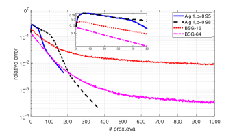
Figure 1: Iteration Complexity of Algorithm1 and BSG

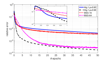
Figure 2: Oracle Complexity of Algorithm1 and BSG

	Algorithm 1, p=0.95	Algorithm 1, p=0.98	BSG-16	BSG-64
emp.err	4.30e-3	1.73e-4	2.60e-3	2.75e-4
prox.eval	178	375	6251	1563
CPU(s)	5.94	10.25	118.65	33.36

Table 4: Comparison of Algorithm 1 and BSG

Influence of block-specific steplengths: In this experiment, we set $N=1000,d=200$, and let the entries of $a_{i}\in\mathbb{R}^{d}$ corresponding to different blocks be generated from normal distributions with zero mean but with differing variances. Such data generation implies that the block-wise Lipschitz constants of ${1\over 2N}\sum_{i=1}^{N}(a_{i}^{T}x-b_{i})^{2}$ can vary. We implement Algorithm 1 with the non-uniform block selection as per a distribution $p_{i}={L_{i}\over\sum_{i=1}^{n}L_{i}}$ in two settings: (i) the same steplength $\alpha_{i}\equiv\alpha={1.28\over L}$ depending on the Lipschtiz constant of $\nabla\bar{f}(x)$, and (ii) the block-specific steplength $\alpha_{i}={1\over L_{i}}$ depending on the block-wise Lipschitz constant $L_{i}.$ Such a selection ensures that the steplengths in two settings are approximately the same when the block-wise Lipschitz constants are identical. For a particular set of realizations with the Lipschtiz constant satisfying $L_{\max}/L_{ave}=2.5$, the empirical iteration and oracle complexity of Algorithm 1 in the two settings are shown in Figures 4 and 4, respectively. These findings reinforce the point that block-specific steplengths, reliant on block-wise Lipschitz constant $L_{i}$, display better empirical behavior since less proximal evaluations (see Figure 4) and less sampled gradients (see Figure 4) are required for obtaining a solution with similar accuracy. In addition, we generate four sets of data, for which the global Lipschitz constant $L$ of the problem (LASSO) is the same while the ratio $L_{\max}/L_{ave}$ is different. We then run Algorithm 1 with the identical and block-specific steplengths on the four generated datasets up to 100 epochs and compare the empirical errors. The results are shown in Table 5, where $x^{I}(K)$ and $x^{B}(K)$ denote the estimates generated by Algorithm 1 with identical and block-specific steplengths, respectively. Since the ratio ${\mathbb{E}[F(x^{I}(K))]-F^{*}\over\mathbb{E}[F(x^{B}(K))]-F^{*}}$ is greater than one, we may conclude that the block-specific steplengths might lead to much better algorithm performance compared with identical steplength. We observe that empirical error can be $50$ times poorer when $L_{\max}/L_{ave}=1.47$.

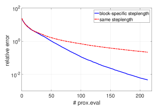
Figure 3: Iteration Complexity of Algorithm 1 with identical and block-specific steplengths

Figure 4: Oracle Complexity of Algorithm 1 with identical and block-specific steplengths

	${L_{\max}\over L_{ave}}=1.15$	${L_{\max}\over L_{ave}}=1.27$	${L_{\max}\over L_{ave}}=1.34$	${L_{\max}\over L_{ave}}=1.47$
${\mathbb{E}[F(x^{I}(K))]-F^{*}\over\mathbb{E}[F(x^{B}(K))]-F^{*}}$	15.3	27.5	31.9	52.4

Table 5: Comparison of Algorithm 1 with identical and block-specific steplengths

Uniform vs non-uniform block selection mechanism. We generate a particular set of realizations with Lipschitz constants of ${1\over 2N}\sum_{i=1}^{N}(a_{i}^{T}x-b_{i})^{2}$ satisfying $L_{\max}/L_{ave}=1.35$. We implement Algorithm 1 with the non-uniform and the uniform block selection probability, while keeping the other algorithm parameters the same. The empirical iteration and oracle complexities are displayed in Fig. 5, showing that non-uniform block selection leads to better performance than the uniform case and reduces the empirical error by approximately 50%.

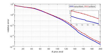
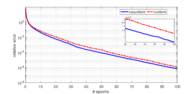
Figure 5: Algorithm 1 with Uniform and Non-uniform Block Selection for (LASSO) with $L_{\max}/L_{ave}=1.35$

Influence of delays. We now compare the empirical performance of Algorithm 1 with and without delays, where in the delayed case, we set the delay to be uniformly bounded by some positive integer. The iteration and oracle complexity bounds are displayed in Fig. 6, which shows that a larger delay leads to worse performance than the case with smaller delay or without delay.

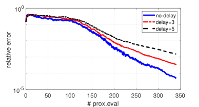
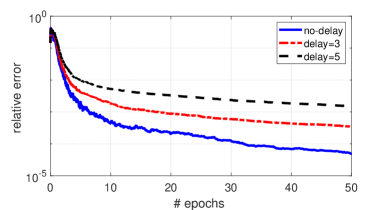
Figure 6: Performance of Algorithm1 with Delays and without Delays

5.2 Nonlinear least squares

We consider a binary classification problem on a data set $\{x_{i},y_{i}\}_{i=1}^{N}$, where $x_{i}\in\mathbb{R}^{d}$ and $y_{i}\in\{0,1\}$ are the $i$th feature vector and the corresponding label, respectively. We consider the minimization of empirical error: $\min\limits_{w,b}{1\over 2N}\sum_{i=1}^{N}\left(y_{i}-\phi(w^{T}x_{i}+b)\right)^{2},$ where $\phi(z)={1\over 1+e^{-z}}$ is the sigmoid function. We apply Algorithm  1 to gisette from LIBSVM library and investigate how batch-sizes influence the training loss and misclassification rate. We partition the vector $w\in\mathbb{R}^{d}$ into $n=10$ blocks. We implement Algorithm 1 with $\alpha=0.2$, where the batch-sizes are set to be the constant batch-sizes $N_{i}(k)\equiv 0.02N,0.05N$ and the increasing batch-sizes $N_{i}(k)=\Gamma_{i}(k),$ $(\Gamma_{i}(k))^{2}$. From Figure 7, we conclude that smaller batch-sizes would lead to better performance if we run the algorithm with a relatively small amount of samples (e.g, $N$); the mini-batch schemes may not perform well if the batch-size is not suitably selected, for instance, $0.05N$. Favorable behavior follows if the batch-size increases at a suitable rate, e.g., linearly.

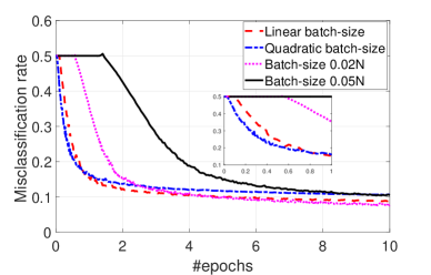
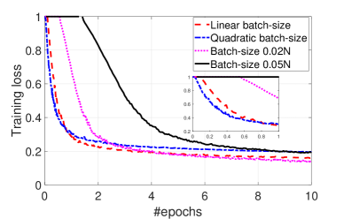
Figure 7: Performance of Algorithm 1 with different batchsizes applied to the classification problem

6 Concluding remarks

Existing block-based techniques for stochastic nonconvex optimization rely on centrally mandated batch-sizes and steplengths bounded by the global Lipschitz constant, leading to larger oracle complexities and poorer performance (because of shorter steps), as well as higher informational coordination requirements. We consider minimizing the sum of an expectation-valued smooth nonconvex function and a nonsmooth separable convex function through a limited coordination asynchronous variance-reduced method, reliant on block-specific steplengths and random decentralized batch-sizes. The almost sure convergence of the generated iterates is established. In addition, the scheme achieves the deterministic rate of $\mathcal{O}(1/K)$ with the rate and oracle complexities dependent on $L_{\rm ave}$ rather than $L_{\max}$. Furthermore, under the proximal PL requirement, the iterates provably converge linearly (polynomially) to the global optimum in a mean sense when batch-sizes grow geometrically (polynomially). Notably, despite using randomized batch-size sequences, we show that the deterministic iteration complexities may be achieved. Specifically, the schemes achieve the optimal oracle complexity when the considered problem admits a single block. Finally, numerical studies are carried out to support the theoretical findings and reveal that schemes leveraging block-specific Lipschitz constants lead to significantly superior empirical behavior.

Appendix A Proof of Lemma 2

Let $x_{-i}$ denote the coordinates of the variable $x$ except those correspond to block $i.$ By applying Lemma 1 to the function $\bar{f}\left(\cdot,x_{-i_{k}}(k)\right)$ and Eqn. (6) with $y=\bar{x}_{i_{k}}(k+1),z=x=x_{i_{k}}(k),$ and $g=\nabla_{x_{i_{k}}}\bar{f}(x(k))$, we obtain the following inequality:

$$\bar{f}\left(x_{-i_{k}}(k),\bar{x}_{i_{k}}(k+1)\right)+r_{i_{k}}(\bar{x}_{i_{k}}(k+1))$$

$$\leq\bar{f}(x(k))+r_{i_{k}}(x_{i_{k}}(k))+\left(\frac{L_{i_{k}}}{2}-{1\over\alpha_{i}}\right)\|\bar{x}_{i_{k}}(k+1)-x_{i_{k}}(k)\|^{2}.$$

Define $\tilde{x}(k+1)$ as follows:

$$\tilde{x}_{i_{k}}(k+1)\triangleq\bar{x}_{i_{k}}(k+1){\rm~{}~{}and~{}~{}}\tilde{x}_{j}(k+1)\triangleq x_{j}(k)~{}\forall j\neq i_{k}.$$ (31)

Then $r_{j}(\tilde{x}_{j}(k+1))=r_{j}(x_{j}(k))~{}\forall j\neq i_{k}$, and hence we obtain the following bound:

$$F\left(\tilde{x}(k+1)\right)\leq F\left(x(k)\right)+\left(\frac{L_{i_{k}}}{2}-{1\over\alpha_{i_{k}}}\right)\|\bar{x}_{i_{k}}(k+1)-x_{i_{k}}(k)\|^{2}.$$ (32)

By applying Lemma 1 to the function $\bar{f}\left(\cdot,x_{-i_{k}}(k)\right)$ and the update (5) with $y=x_{i_{k}}(k+1),z=\bar{x}_{i_{k}}(k+1),x=x_{i_{k}}(k),$ and $g=\nabla_{x_{i_{k}}}\bar{f}(x(k))+w_{i_{k}}(k+1)$, one obtains

$$\begin{split}&\bar{f}\left(x_{-i_{k}}(k),x_{i_{k}}(k+1)\right)+r_{i_{k}}(x_{i_{k}}(k+1))\leq\bar{f}\left(x_{-i_{k}}(k),\bar{x}_{i_{k}}(k+1)\right)+r_{i_{k}}(\bar{x}_{i_{k}}(k+1))\\ &-(x_{i_{k}}(k+1)-\bar{x}_{i_{k}}(k+1))^{T}w_{i_{k}}(k+1)+\left(\frac{L_{i_{k}}}{2}-{1\over 2\alpha_{i_{k}}}\right)\|x_{i_{k}}(k+1)-x_{i_{k}}(k)\|^{2}\\ &+\left(\frac{L_{i_{k}}}{2}+{1\over 2\alpha_{i_{k}}}\right)\|\bar{x}_{i_{k}}(k+1)-x_{i_{k}}(k)\|^{2}-{1\over 2\alpha_{i_{k}}}\|x_{i_{k}}(k+1)-\bar{x}_{i_{k}}(k+1)\|^{2}.\end{split}$$

Note that $\tilde{x}_{j}(k+1)=x_{j}(k)~{}\forall j\neq i_{k}$ and $\tilde{x}_{i_{k}}(k+1)=\bar{x}_{i_{k}}(k+1)$ by definition (31). Then by the definition of $F(\cdot)$, we have the following

$$\begin{split}&F(x(k+1))\leq F(\tilde{x}(k+1))-(x_{i_{k}}(k+1)-\bar{x}_{i_{k}}(k+1))^{T}w_{i_{k}}(k+1)\\ &+\left(\frac{L_{i_{k}}}{2}-{1\over 2\alpha_{i_{k}}}\right)\|x_{i_{k}}(k+1)-x_{i_{k}}(k)\|^{2}-{1\over 2\alpha_{i_{k}}}\|x_{i_{k}}(k+1)-\bar{x}_{i_{k}}(k+1)\|^{2}\\ &+\left(\frac{L_{i_{k}}}{2}+{1\over 2\alpha_{i_{k}}}\right)\|\bar{x}_{i_{k}}(k+1)-x_{i_{k}}(k)\|^{2}.\end{split}$$ (33)

By recalling that $-a^{T}b\leq{1\over 2\alpha}\|a\|^{2}+{\alpha\over 2}\|b\|^{2}$, the following holds:

$$\begin{split}&-(x_{i_{k}}(k+1)-\bar{x}_{i_{k}}(k+1))^{T}w_{i_{k}}(k+1)\\ &\leq{1\over 2\alpha_{i_{k}}}\|x_{i_{k}}(k+1)-\bar{x}_{i_{k}}(k+1)\|^{2}+{\alpha_{i_{k}}\over 2}\|w_{i_{k}}(k+1)||^{2}.\end{split}$$ (34)

Therefore, by substituting (34) into (33), we obtain the following bound:

$$\begin{split}F(x(k+1))&\leq F(\tilde{x}(k+1))+\left(\frac{L_{i_{k}}}{2}-{1\over 2\alpha_{i_{k}}}\right)\|x_{i_{k}}(k+1)-x_{i_{k}}(k)\|^{2}\\ &+\left(\frac{L_{i_{k}}}{2}+{1\over 2\alpha_{i_{k}}}\right)\|\bar{x}_{i_{k}}(k+1)-x_{i_{k}}(k)\|^{2}+{\alpha_{i_{k}}\over 2}\|w_{i_{k}}(k+1)||^{2}.\end{split}$$ (35)

By adding inequalities (32) and (35),

$$\begin{split}F(x(k+1))&\leq F\left(x(k)\right)+\left(\frac{L_{i_{k}}}{2}-{1\over 2\alpha_{i_{k}}}\right)\|x_{i_{k}}(k+1)-x_{i_{k}}(k)\|^{2}\\ &+{\alpha_{i_{k}}\over 2}\|w_{i_{k}}(k+1)||^{2}+\left(L_{i_{k}}-{1\over 2\alpha_{i_{k}}}\right)\|\bar{x}_{i_{k}}(k+1)-x_{i_{k}}(k)\|^{2}.\end{split}$$ (36)

Note that for all $i=1,\cdots,n,$ $\frac{L_{i}}{2}-{1\over 2\alpha_{i}}\leq 0$ by $\alpha_{i}\leq{1\over L_{i}}$. Then the second term on the right-hand side of Eqn. (36) is nonpositive, hence we can take out this term from the upper bound of $F(x(k+1))$. Since $x(k)$ is adapted to $\mathcal{F}_{k}$, by taking expectations conditioned on $\mathcal{F}_{k}$ on both sides of (36), we obtain that

$$\begin{split}\mathbb{E}\big{[}F(x(k+1))|\mathcal{F}_{k}\big{]}&\leq F(x(k))+\mathbb{E}\left[\left(L_{i_{k}}-{1\over 2\alpha_{i_{k}}}\right)\|\bar{x}_{i_{k}}(k+1)-x_{i_{k}}(k)\|^{2}|\mathcal{F}_{k}\right]\\ &+{1\over 2}\mathbb{E}\big{[}\alpha_{i_{k}}\|w_{i_{k}}(k+1)||^{2}|\mathcal{F}_{k}\big{]}.\end{split}$$ (37)

Note that for any $i\in\mathcal{N}$, $\bar{x}_{i}(k+1)$ is adapted to $\mathcal{F}_{k}$ by the definition (6), and $i_{k}$ is independent of $\mathcal{F}_{k}$ by Assumption 2(ii). Therefore, by [5, Corollary 7.1.2 ] and $\mathbb{P}(i_{k}=i)=p_{i}$, the following holds a.s.:

$$\mathbb{E}\left[\left(L_{i_{k}}-{1\over 2\alpha_{i_{k}}}\right)\|\bar{x}_{i_{k}}(k+1)-x_{i_{k}}(k)\|^{2}|\mathcal{F}_{k}\right]=\sum_{i=1}^{n}p_{i}\left(L_{i}-{1\over 2\alpha_{i}}\right)\|\bar{x}_{i}(k+1)-x_{i}(k)\|^{2}.$$ (38)

Then by substituting (38) into (37), we obtain Eqn. (7). $\Box$

Appendix B Proof of Lemma 3.

By recalling that the gradient map $\nabla_{x_{i}}\bar{f}(x)$ is $L_{i}$-Lipschitz continuous from Assumption 1(ii) and that $\tilde{x}_{j}(k+1)=x_{j}(k)~{}\forall j\neq i_{k}$ by definition (31), we have the following inequality:

$$\bar{f}(\tilde{x}(k+1))\leq\bar{f}(x(k))+(\tilde{x}_{i_{k}}(k+1)-x_{i_{k}}(k))^{T}\nabla_{x_{i_{k}}}\bar{f}(x(k))+{L_{i_{k}}\over 2}\|\tilde{x}_{i_{k}}(k+1)-x_{i_{k}}(k)\|^{2}.$$

Using the definition of $\tilde{x}_{k+1}$ in (31), we have that $r_{j}\left(\tilde{x}_{j}(k+1)\right)=r_{j}(x_{j}(k))~{}\forall j\neq i_{k}$, $\tilde{x}_{i_{k}}(k+1)=\bar{x}_{i_{k}}(k+1)$. Thus, the the following relation holds

$$F(\tilde{x}(k+1)) \leq F(x(k))+(\tilde{x}_{i_{k}}(k+1)-x_{i_{k}}(k))^{T}\nabla_{x_{i_{k}}}\bar{f}(x(k))+{L_{i_{k}}\over 2}\|\tilde{x}_{i_{k}}(k+1)-x_{i_{k}}(k)\|^{2}$$

$$\quad+r_{i_{k}}(\tilde{x}_{i_{k}}(k+1))-r_{i_{k}}(x_{i_{k}}(k))$$

$$\leq F(x(k))+(\bar{x}_{i_{k}}(k+1)-x_{i_{k}}(k))^{T}\nabla_{x_{i_{k}}}\bar{f}(x(k))$$

$$\quad+{1\over 2\alpha_{i_{k}}}\|\bar{x}_{i_{k}}(k+1)-x_{i_{k}}(k)\|^{2}+r_{i_{k}}(\bar{x}_{i_{k}}(k+1))-r_{i_{k}}(x_{i_{k}}(k)),$$ (39)

where the last inequality holds by $\alpha_{i}<1/L_{i}~{}\forall i\in\mathcal{N}.$ Since for any $i\in\mathcal{N},$ $\bar{x}_{i}(k+1)$ is adapted to $\mathcal{F}_{k}$ by its definition (6), and $i_{k}$ is independent of $\mathcal{F}_{k}$. Then, by [5, Corollary 7.1.2 ] and $\mathbb{P}(i_{k}=i)=p_{i}$, we have that

$$\mathbb{E}\Big{[}(\bar{x}_{i_{k}}(k+1)-x_{i_{k}}(k))^{T}\nabla_{x_{i_{k}}}\bar{f}(x(k))+{\|\bar{x}_{i_{k}}(k+1)-x_{i_{k}}(k)\|^{2}/(2\alpha_{i_{k}})}+r_{i_{k}}(\bar{x}_{i_{k}}(k+1))-r_{i_{k}}(x_{i_{k}}(k))\big{|}\mathcal{F}_{k}\Big{]}$$

$$=\sum_{i=1}^{n}p_{i}\Big{(}(\bar{x}_{i}(k+1)-x_{i}(k))^{T}\nabla_{x_{i}}\bar{f}(x(k))+{1\over 2\alpha_{i}}\|\bar{x}_{i}(k+1)-x_{i}(k)\|^{2}+r_{i}(\bar{x}_{i}(k+1))-r_{i}(x_{i}(k))\Big{)}$$

$${{\scriptstyle\eqref{def-xbar}}\atop=}\sum_{i=1}^{n}p_{i}\min_{y_{i}\in\mathbb{R}^{d_{i}}}\Big{[}\nabla_{x_{i}}\bar{f}(x(k))^{T}(y_{i}-x_{i}(k))+{1\over 2\alpha_{i}}\|y_{i}-x_{i}(k)\|^{2}+r_{i}(y_{i})-r_{i}(x_{i}(k))\Big{]}$$

$$\leq p_{\min}\sum_{i=1}^{n}\min_{y_{i}\in\mathbb{R}^{d_{i}}}\Big{[}\nabla_{x_{i}}\bar{f}(x(k))^{T}(y_{i}-x_{i}(k))+{1\over 2\alpha_{i}}\|y_{i}-x_{i}(k)\|^{2}+r_{i}(y_{i})-r_{i}(x_{i}(k))\Big{]},$$

where the last inequality follows by $\min_{y_{i}\in\mathbb{R}^{d_{i}}}[\nabla_{x_{i}}\bar{f}(x(k))^{T}(y_{i}-x_{i}(k))+{1\over 2\alpha_{i}}\|y_{i}-x_{i}(k)\|^{2}+r_{i}(y_{i})-r_{i}(x_{i}(k))]\leq 0$. Then by $\alpha_{i}^{-1}\leq\alpha_{\min}^{-1}$ and Assumption 3, the above equation is further bounded by

$$\begin{split}&p_{\min}\sum_{i=1}^{n}\min_{y_{i}\in\mathbb{R}^{d_{i}}}\Big{[}\nabla_{x_{i}}\bar{f}(x(k))^{T}(y_{i}-x_{i}(k))+{1\over 2\alpha_{\min}}\|y_{i}-x_{i}(k)\|^{2}+r_{i}(y_{i})-r_{i}(x_{i}(k))\Big{]}\\ &=-{p_{\min}\alpha_{\min}\over 2}D_{r}(x(k),\alpha_{\min}^{-1})\leq-{\alpha_{\min}p_{\min}\over 2}D_{r}(x(k),L_{\max})\\ &\leq-{\alpha_{\min}\mu p_{\min}}\big{(}F(x(k))-F^{*}\big{)},\end{split}$$ (40)

where the first inequality follows from [17, Lemma 1] since $D_{r}(x,\cdot)$ is nonnegative and nondecreasing in $(0,\infty)$ and $\alpha_{\min}^{-1}\geq L_{\max}$. Then by taking unconditional expectations on both sides of (B) and using (40), we obtain that

$$\begin{split}\mathbb{E}\big{[}F(\tilde{x}(k+1))\big{]}&\leq\mathbb{E}\big{[}F(x(k))\big{]}-\alpha_{\min}\mu p_{\min}\mathbb{E}\big{[}F(x(k))-F^{*}\big{]}.\end{split}$$ (41)

By taking unconditional expectations on both sides of (32) and using $\mathbb{P}(i_{k}=i)=p_{i}$, we obtain

$$\mathbb{E}\big{[}F\left(\tilde{x}(k+1)\right)\big{]}\leq\mathbb{E}\big{[}F(x(k))\big{]}+\sum_{i=1}^{n}p_{i}\left({L_{i}\over 2}-{1\over\alpha_{i}}\right)\|\bar{x}_{i}(k+1)-x_{i}(k)\|^{2}.$$ (42)

Adding $(1-\beta)\times$ (41) to $\beta\times$ (42) with $\beta\in(0.5,1)$, we obtain the following inequality:

$$\begin{split}\mathbb{E}\big{[}F(\tilde{x}(k+1))\big{]}&\leq\mathbb{E}\big{[}F(x(k))\big{]}+\beta\sum_{i=1}^{n}p_{i}\left({L_{i}\over 2}-{1\over\alpha_{i}}\right)\|\bar{x}_{i}(k+1)-x_{i}(k)\|^{2}\\ &-{\alpha_{\min}(1-\beta)\mu p_{\min}}\mathbb{E}\big{[}F(x(k))-F^{*}\big{]}.\end{split}$$ (43)

Using $\alpha_{i}<{1\over L_{i}},$ Assumption 2, and $\mathbb{P}(i_{k}=i)=p_{i}$, and by taking unconditional expectations on both sides of (35), the following holds:

$$\begin{split}\mathbb{E}\big{[}F(x_{k+1})\big{]}&\leq\mathbb{E}\big{[}F(\tilde{x}(k+1))\big{]}\\ &\quad+\sum_{i=1}^{n}p_{i}\left({L_{i}\over 2}+{1\over 2\alpha_{i}}\right)\|\bar{x}_{i}(k+1)-x_{i}(k)\|^{2}+{\sigma^{2}\over 2}\sum_{i=1}^{n}\alpha_{i}p_{i}\mathbb{E}\left[N_{i}(k)^{-1}\right].\end{split}$$ (44)

Therefore, by adding inequality (44) to (43) yields the following bound:

$$\mathbb{E}\big{[}F(x(k+1))\big{]} \leq\mathbb{E}\big{[}F(x(k))\big{]}+\sum_{i=1}^{n}p_{i}\left(\frac{L_{i}(1+\beta)}{2}-{2\beta-1\over 2\alpha_{i}}\right)\|\bar{x}_{i}(k+1)-x_{i}(k)\|^{2}$$

$$-{\alpha_{\min}(1-\beta)\mu p_{\min}}\mathbb{E}\big{[}F(x(k))-F^{*}\big{]}+{\sigma^{2}\over 2}\sum_{i=1}^{n}\alpha_{i}p_{i}\mathbb{E}\left[N_{i}(k)^{-1}\right].$$ (45)

By recalling that $0<\alpha_{i}\leq{2\beta-1\over L_{i}(1+\beta)}$, we get $\frac{L_{i}(1+\beta)}{2}-{2\beta-1\over 2\alpha_{i}}\leq 0.$ Thus, by subtracting $F^{*}$ from both sides of (B), we obtain (19). $\Box$

References

- [1] H. Attouch, J. Bolte, and B.F. Svaiter, Convergence of descent methods for semi-algebraic and tame problems: proximal algorithms, forward–backward splitting, and regularized Gauss–Seidel methods, Mathematical Programming 137 (2013), pp. 91–129.
- [2] A. Beck and M. Teboulle, A fast iterative shrinkage-thresholding algorithm for linear inverse problems, SIAM journal on imaging sciences 2 (2009), pp. 183–202.
- [3] S. Boyd, A. Ghosh, B. Prabhakar, and D. Shah, Randomized gossip algorithms, IEEE/ACM Transactions on Networking (TON) 14 (2006), pp. 2508–2530.
- [4] G.H. Chen and R.T. Rockafellar, Convergence rates in forward–backward splitting, SIAM Journal on Optimization 7 (1997), pp. 421–444.
- [5] Y.S. Chow and H. Teicher, Probability theory: independence, interchangeability, martingales, Springer Science & Business Media, 2012.
- [6] P.L. Combettes and J.C. Pesquet, Proximal splitting methods in signal processing, in Fixed-point algorithms for inverse problems in science and engineering, Springer, 2011, pp. 185–212.
- [7] D. Csiba and P. Richtárik, Global convergence of arbitrary-block gradient methods for generalized Polyak–Łojasiewicz functions, arXiv preprint arXiv:1709.03014 (2017).
- [8] C.D. Dang and G. Lan, Stochastic block mirror descent methods for nonsmooth and stochastic optimization, SIAM Journal on Optimization 25 (2015), pp. 856–881.
- [9] D. Davis, The asynchronous palm algorithm for nonsmooth nonconvex problems, arXiv preprint arXiv:1604.00526 (2016).
- [10] D. d’Esopo, A convex programming procedure, Naval Research Logistics Quarterly 6 (1959), pp. 33–42.
- [11] O. Fercoq and P. Richtárik, Accelerated, parallel, and proximal coordinate descent, SIAM Journal on Optimization 25 (2015), pp. 1997–2023.
- [12] P. Frankel, G. Garrigos, and J. Peypouquet, Splitting methods with variable metric for Kurdyka–Łojasiewicz functions and general convergence rates, Journal of Optimization Theory and Applications 165 (2015), pp. 874–900.
- [13] S. Ghadimi and G. Lan, Accelerated gradient methods for nonconvex nonlinear and stochastic programming, Math. Programming 156 (2016), pp. 59–99.
- [14] S. Ghadimi, G. Lan, and H. Zhang, Mini-batch stochastic approximation methods for nonconvex stochastic composite optimization, Math. Programming 155 (2016), pp. 267–305.
- [15] A. Jalilzadeh, U.V. Shanbhag, J.H. Blanchet, and P.W. Glynn, Optimal smoothed variable sample-size accelerated proximal methods for structured nonsmooth stochastic convex programs, arXiv preprint arXiv:1803.00718 (2018).
- [16] A. Jofré and P. Thompson, On variance reduction for stochastic smooth convex optimization with multiplicative noise, arXiv preprint arXiv:1705.02969 (2017).
- [17] H. Karimi, J. Nutini, and M. Schmidt, Linear convergence of gradient and proximal-gradient methods under the Polyak-Łojasiewicz condition, in Joint European Conference on Machine Learning and Knowledge Discovery in Databases. Springer, 2016, pp. 795–811.
- [18] J. Koshal, A. Nedić, and U.V. Shanbhag, Distributed algorithms for aggregative games on graphs, Operations Research 64 (2016), pp. 680–704.
- [19] J. Lei and U.V. Shanbhag, Asynchronous schemes for stochastic and misspecified potential games and nonconvex optimization, Accepted for publication at Operations Research, arXiv:1711.03963 (2019).
- [20] J. Lei and U. V. Shanbhag, Distributed variable sample-size gradient-response and best-response schemes for stochastic nash games over graphs, arXiv:1811.11246 (2018).
- [21] P.L. Lions and B. Mercier, Splitting algorithms for the sum of two nonlinear operators, SIAM Journal on Numerical Analysis 16 (1979), pp. 964–979.
- [22] H. Mine and M. Fukushima, A minimization method for the sum of a convex function and a continuously differentiable function, Journal of Optimization Theory and Applications 33 (1981), pp. 9–23.
- [23] Y. Nesterov, Efficiency of coordinate descent methods on huge-scale optimization problems, SIAM Journal on Optimization 22 (2012), pp. 341–362.
- [24] A. Papoulis, Probability, random variables and stochastic theory (1984).
- [25] N. Parikh, S. Boyd, et al., Proximal algorithms, Foundations and Trends® in Optimization 1 (2014), pp. 127–239.
- [26] Z. Peng, T. Wu, Y. Xu, M. Yan, and W. Yin, Coordinate friendly structures, algorithms and applications, arXiv preprint arXiv:1601.00863 (2016).
- [27] B.T. Polyak, Gradient methods for minimizing functionals, Zhurnal Vychislitel’noi Matematiki i Matematicheskoi Fiziki 3 (1963), pp. 643–653.
- [28] M. Razaviyayn, M. Hong, and Z.Q. Luo, A unified convergence analysis of block successive minimization methods for nonsmooth optimization, SIAM Journal on Optimization 23 (2013), pp. 1126–1153.
- [29] S.J. Reddi, A. Hefny, S. Sra, B. Póczos, and A. Smola, Stochastic variance reduction for nonconvex optimization, in International conference on machine learning. 2016, pp. 314–323.
- [30] S.J. Reddi, S. Sra, B. Póczos, and A. Smola, Fast incremental method for smooth nonconvex optimization, in Decision and Control (CDC), 2016 IEEE 55th Conference on. IEEE, 2016, pp. 1971–1977.
- [31] S.J. Reddi, S. Sra, B. Póczos, and A.J. Smola, Proximal stochastic methods for nonsmooth nonconvex finite-sum optimization, in Advances in Neural Information Processing Systems. 2016, pp. 1145–1153.
- [32] P. Richtárik and M. Takáč, Iteration complexity of randomized block-coordinate descent methods for minimizing a composite function, Math. Programming 144 (2014), pp. 1–38.
- [33] H. Robbins and D. Siegmund, A convergence theorem for nonnegative almost supermartingales and some applications, in H. Robbins Selected Papers, Springer, 1985, pp. 111–135.
- [34] R.T. Rockafellar, Monotone operators and the proximal point algorithm, SIAM journal on control and optimization 14 (1976), pp. 877–898.
- [35] L. Rosasco, S. Villa, and B.C. Vũ, Convergence of stochastic proximal gradient algorithm, arXiv preprint arXiv:1403.5074 (2014).
- [36] U.V. Shanbhag and J.H. Blanchet, Budget-constrained stochastic approximation, in Winter Simulation Conference (WSC), 2015. IEEE, 2015, pp. 368–379.
- [37] U.V. Shanbhag, J.S. Pang, and S. Sen, Inexact best-response schemes for stochastic Nash games: linear convergence and Iteration complexity analysis, in Decision and Control (CDC), 2016 IEEE 55th Conference on. IEEE, 2016, pp. 3591–3596.
- [38] P. Tseng, A modified forward-backward splitting method for maximal monotone mappings, SIAM Journal on Control and Optimization 38 (2000), pp. 431–446.
- [39] P. Tseng, Convergence of a block coordinate descent method for nondifferentiable minimization, Journal of optimization theory and applications 109 (2001), pp. 475–494.
- [40] G. Wang and G. Giannakis, Solving random systems of quadratic equations via truncated generalized gradient flow, in Advances in Neural Information Processing Systems. 2016, pp. 568–576.
- [41] G. Wang, G.B. Giannakis, and J. Chen, Scalable solvers of random quadratic equations via stochastic truncated amplitude flow, IEEE Transactions on Signal Processing 65 (2017), pp. 1961–1974.
- [42] L. Xiao and T. Zhang, A proximal stochastic gradient method with progressive variance reduction, SIAM Journal on Optimization 24 (2014), pp. 2057–2075.
- [43] Y. Xu and W. Yin, A block coordinate descent method for regularized multiconvex optimization with applications to nonnegative tensor factorization and completion, SIAM Journal on imaging sciences 6 (2013), pp. 1758–1789.
- [44] Y. Xu and W. Yin, Block stochastic gradient iteration for convex and nonconvex optimization, SIAM Journal on Optimization 25 (2015), pp. 1686–1716.
- [45] Y. Xu and W. Yin, A globally convergent algorithm for nonconvex optimization based on block coordinate update, Journal of Scientific Computing (2017), pp. 1–35.
- [46] P. Yi and L. Pavel, Asynchronous distributed algorithms for seeking generalized nash equilibria under full and partial-decision information, IEEE transactions on cybernetics (2019).
- [47] F. Yousefian, A. Nedić, and U.V. Shanbhag, On stochastic mirror-prox algorithms for stochastic Cartesian variational inequalities: Randomized block coordinate and optimal averaging schemes, Set-Valued and Variational Analysis (2018).