The Radio Ammonia Mid-plane Survey (RAMPS) Pilot Survey

Abstract

The Radio Ammonia Mid-Plane Survey (RAMPS) is a molecular line survey that aims to map a portion of the Galactic midplane in the first quadrant of the Galaxy ($l=10^{\circ}-40^{\circ}$, $\lvert b\rvert\leq 0.4^{\circ}$) using the Green Bank Telescope. We present results from the pilot survey, which has mapped approximately 6.5 square degrees in fields centered at $l=10^{\circ},\ 23^{\circ},\ 24^{\circ},\ 28^{\circ},\ 29^{\circ},\ 30^{\circ},\ 31^{\circ},\ 38^{\circ},\ 45^{\circ},\ \mathrm{and}\ 47^{\circ}$. RAMPS observes the $\mathrm{NH_{3}}$ inversion transitions $\mathrm{NH_{3}(1,1)-(5,5)}$, the $\mathrm{H_{2}O}\ 6_{1,6}-5_{2,3}$ maser line at 22.235 GHz, and several other molecular lines. We present a representative portion of the data from the pilot survey, including $\mathrm{NH_{3}(1,1)}$ and $\mathrm{NH_{3}(2,2)}$ integrated intensity maps, $\mathrm{H_{2}O}$ maser positions, maps of $\mathrm{NH_{3}}$ velocity, $\mathrm{NH_{3}}$ line width, total $\mathrm{NH_{3}}$ column density, and $\mathrm{NH_{3}}$ rotational temperature. These data and the data cubes from which they were produced are publicly available on the RAMPS website.

We begin by discussing the survey and its observations (Section 2). Subsequently, we present the results of the RAMPS pilot survey (Section 3). We then present a preliminary analysis of the data (Section LABEL:sec:analysis) and a comparison of the features of the RAMPS survey to those of previous surveys (Section LABEL:sec:comparison). Finally, we summarize our conclusions (Section LABEL:sec:conclusion).

2 The Survey

RAMPS is a blind molecular line survey that targets a portion of the Galactic midplane in the first quadrant of the Galaxy. In this section, we describe in detail the survey and the processing of the data. In Section 2.1, we discuss the observed lines. In Section 2.2, we describe the telescope, receiver, and spectrometer. In Section 2.3, we introduce our observing strategy. In Section 2.4, we outline the data reduction pipeline. In Section 2.5, we describe the post-reduction processing of the data. Then, in Section 2.6, we detail the public release of the data.

2.1 Line Selection

RAMPS observes 13 molecular transitions, which we present in Table 1. The most frequently detected lines, and the lines we limit our focus to in the current paper, are $\mathrm{NH_{3}}$ (1,1), $\mathrm{NH_{3}}$ (2,2), and the $\mathrm{H_{2}O}\ 6_{1,6}-5_{2,3}$ maser line.

The $\mathrm{NH_{3}}$ inversion transitions near 23 GHz are particularly well suited to the study of high-mass stars. In addition to having a large critical density ($n_{\rm{crit}}\sim 3\times 10^{3}\ \mathrm{cm^{-3}}$) and revealing kinematic information, the $\mathrm{NH_{3}}$ inversion transitions provide a robust estimate of the gas temperature and the column density. The excitation temperature (also called the rotational temperature) representing a series of $\mathrm{NH_{3}}$ rotational transitions for an observed source of emission is set by the $\mathrm{NH_{3}}$ level populations. For gas with a density well above the critical density, the rotational temperature is equal to the gas temperature. Thus, in LTE one can determine the gas temperature from the brightness ratios of the inversion lines. We can measure column density from the relative intensities of the nuclear quadrupole hyperfine lines since the intensity ratios of the satellite hyperfine lines to the main hyperfine line are set by the optical depth.

The collisionally pumped $\mathrm{H_{2}O}$ maser line at 22.235 GHz (1989ApJ...346..983E) is useful because it is known to trace active star formation. Although the exact evolutionary stage or stages probed by $\mathrm{H_{2}O}$ masers in star-forming clumps remain uncertain (2010MNRAS.405.2471V), $\mathrm{H_{2}O}$ masers are frequently found in high-mass SFRs. They are, however, also seen toward low-mass SFRs. Given that $\mathrm{H_{2}O}$ can be one of the brightest spectral lines emitting from low-mass SFRs, these masers can help us detect low-mass SFRs at much larger distances than continuum surveys. $\mathrm{H_{2}O}$ masers are also associated with asymptotic giant branch (AGB) stars, which can be observed using VLBI techniques to study the dynamics of their atmospheres and winds (1997PASP..109.1286M; 2008PASJ...60.1077S). Furthermore, masers are well suited for parallax measurements (2014ApJ...783..130R) since they are extremely luminous compact sources. Consequently, $\mathrm{H_{2}O}$ masers are particularly useful for measuring accurate distances to SFRs throughout the Galaxy.

The RAMPS spectral setup also includes two shock-excited $\mathrm{CH_{3}OH}$ lines and high-density tracing lines of $\mathrm{HC_{5}N}$, $\mathrm{HC_{7}N}$, and HNCO, as well as CCS, which is found in SFRs that are in an early evolutionary state (1992ApJ...392..551S).

Table 1: The 13 molecular lines observed by RAMPS.

Molecule	Transition	Frequency	$\mathrm{E_{upper}/k}$	Number of
		(MHz)	(K)	Receivers
$\mathrm{NH_{3}}$	($J,K$) = (1,1)	23694.47	23	7
$\mathrm{NH_{3}}$	($J,K$) = (2,2)	23722.60	64	7
$\mathrm{NH_{3}}$	($J,K$) = (3,3)	23870.08	124	7
$\mathrm{NH_{3}}$	($J,K$) = (4,4)	24139.35	201	7
$\mathrm{NH_{3}}$	($J,K$) = (5,5)	24532.92	295	7
$\mathrm{CH_{3}OH}$	$\mathrm{J_{K_{p}}}$ = $10_{1}$ – $9_{2}\ A^{-}$	23444.78	143	7
$\mathrm{HC_{5}N}$	$J$ = 9 – 8	23963.90	6	7
$\mathrm{HC_{5}N}$	$J$ = 8 – 7	21301.26	5	1
$\mathrm{HC_{7}N}$	$J$ = 19 – 18	21431.93	10	1
$\mathrm{CH_{3}OH}$	$\mathrm{J_{K_{p}}}$ = $12_{2}$ – $11_{1}\ A^{-}$	21550.34	479	1
HNCO	$\mathrm{J_{K_{p},K_{o}}}$ = $1_{0,1}-0_{0,0}$	21981.57	1	1
$\mathrm{H_{2}O}$	$\mathrm{J_{K_{p},K_{o}}}$ = $6_{1,6}-5_{2,3}$	22235.08	644	1
CCS	$J$ = 2 – 1	22344.03	2	1

Note. — The quantum numbers given in the $``$Transition” column are $J$, the rotational quantum number, $K$, the projection of $J$ along the molecular axis of symmetry, $K_{\rm{p}}$, the value of $K$ in the limiting case of a prolate spheroid molecule, and $K_{\rm{o}}$, the value of $K$ in the limiting case of an oblate spheroid molecule. $\mathrm{CH_{3}OH}$ $12_{2}-11_{1}\ A^{-}$ is a rotational transition within the first vibrationally excited state, i.e. $v=1$.

2.2 Instrumentation

We performed observations for RAMPS using the 100 m diameter Robert C. Byrd GBT (P09) at the NRAO,, which operates in a nearly continuous frequency range of 0.29 $-$ 115 GHz. The GBT is the most sensitive fully steerable single-dish telescope in the world, which allows us to observe a large area with high spatial resolution. RAMPS uses the $K$-band Focal Plane Array (KFPA; 2008ursi.confE...2M), which is a seven-element receiver array that operates in a frequency range of 18-27.5 GHz. Each receiver has a beam pattern that is well represented by a Gaussian with a $32\arcsec$ FWHM at the rest frequency of $\mathrm{NH_{3}}$(1,1) and a beam-to-beam distance of approximately $95\arcsec$ (Figure 1). The receivers feed into the VErsatile GBT Astronomical Spectrometer (VEGAS; 2012arXiv1202.0938A), a spectrometer equipped for use with focal plane arrays. VEGAS is capable of processing up to 1.25 GHz bandwidth from eight spectrometer banks, each with eight dual polarized sub-bands.

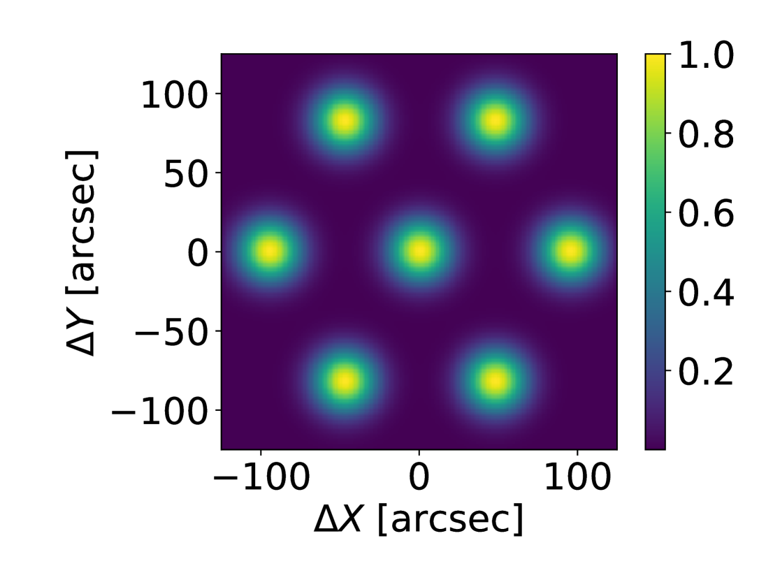
Figure 1: Beam pattern of the KFPA. The color represents the sensitivity as a function of angle relative to the sensitivity at beam center. Each receiver has a Gaussian beam shape with an FWHM of $32\arcsec$ at the rest frequency of $\mathrm{NH_{3}}$(1,1), and the beam-to-beam distance is $\sim 95\arcsec$.

2.3 Observations

In 2014, RAMPS was awarded 210 hr of observing time on the GBT for a pilot survey. The purpose of the pilot survey was to test the feasibility of the RAMPS project and to help commission VEGAS. We performed observations for the RAMPS pilot study between 2014 March 16 and 2015 January 22. We used all seven of the KFPA’s receivers, with 13 dual polarized sub-bands and 23 MHz bandwidth per sub-band. We observed with the $``$medium” spectral resolution, providing a channel width of 1.4 kHz ($\sim 0.018\ \mathrm{km\ s^{-1}}$). We performed Doppler tracking using the $\mathrm{NH_{3}}$(1,1) rest frequency.

While the KFPA has seven available receivers, the VEGAS back end supports eight spectrometer banks. Hence, six of the seven KFPA receivers each feed into an individual spectrometer bank, while the central receiver feeds into two spectrometer banks. We observed the $\mathrm{NH_{3}}$ inversion transitions, $\mathrm{NH_{3}}$(1,1)$-$(5,5), with all seven receivers to achieve better sensitivity for the $\mathrm{NH_{3}}$ data. We observed the 22.235 GHz $\mathrm{H_{2}O}$ maser line with only the central receiver. Although this significantly reduced the sensitivity of our $\mathrm{H_{2}O}$ observations, $\mathrm{H_{2}O}$ masers are typically bright, and thus the GBT frequently detected this line. As discussed in Section 2.1, RAMPS also observed several other lines; the numbers of receivers used to observe each of these spectral lines are indicated in Table 1.

The proposed RAMPS region extends from Galactic longitude $10^{\circ}$ to $40^{\circ}$ and from Galactic latitude $-0^{\circ}.4$ to $+0^{\circ}.4$. The survey region is broken up into $1^{\circ}\times 0^{\circ}.8$ $``$fields” centered on integer-valued Galactic latitudes and $0^{\circ}$ Galactic longitude. We also observed a portion of two additional fields centered on Galactic longitudes $45^{\circ}$ and $47^{\circ}$, due to the presence of several infrared dark clouds of interest. For the first two fields observed in the pilot survey, centered at $l=\mathrm{10^{\circ}\ and\ 30^{\circ}}$, we tested two different mapping schemes. The first of these divides the mapped field into rectangular $``$tiles” of size $0^{\circ}.25\times 0^{\circ}.20$, and the second divides the field into $``$strips” of size $1^{\circ}\times 0^{\circ}.058$. The two schemes differ considerably in the quality of the resulting maps, mainly due to gain variations caused by differing elevations and weather conditions. Due to the long, thin shape of the strips, clumps are often too large to fit completely within a single strip. A clump that was observed in two separate strips was thus observed in different weather conditions and at different elevations. Once the separate observations were combined to create a larger map, this resulted in $``$striping” artifacts in the mapping direction. Given that clumps usually fit completely within tiles, gain variations were less problematic for the tile division scheme. Consequently, we chose to map the rest of the survey region with tiles. After the initial tests of the tiling scheme, we adjusted the parameters for the size and position of the tiles to optimize the sensitivity in the overlap regions between adjacent tiles and fields. Specifically, we increased the tile size to $0^{\circ}.26\times 0^{\circ}.208$ and performed additional observations at the overlap regions between the fields already observed.

We observed in on-the-fly mapping mode, scanning in Galactic longitude, with 4 integrations beam^-1, 1 s integrations, and $0^{\circ}.008$ between rows. Due to these mapping parameters, the sampling of a tile is uneven. In addition, the sampling pattern is dependent on the angle of the KFPA with respect to the Galactic plane. The uneven sampling pattern and its dependence on the array angle are displayed in Figures 2 and 3, which show the expected integration time for each spectrum in a data cube assuming the KFPA configuration displayed in the lower left corner of each map. The angle of the array depends on the target position; thus, different tiles may be mapped with the array at a different angle. Observing an individual tile takes approximately 1 hr. Before mapping a tile, we adjust the pointing and focus of the telescope by observing a known calibrator with flux greater than 3 Jy in the $K$ band. This meets the suggested pointing calibration frequency of once per hour and provides a typical pointing error of $\sim 5\arcsec$. Before observing a new field, we also perform a single pointed observation ($``$on/off”) toward one of the brightest BGPS 1.1 mm sources in the field. This observation serves as a test to ensure that the receiver and back end are configured correctly, as well as a way to evaluate system performance and repeatability over the observing season. A reference $``$off” observation is taken at an offset of $+1^{\circ}$ in Galactic latitude from the tile center immediately before and after mapping in order to subtract atmospheric emission. Although we did not check the “off” positions for emission, we found no evidence of a persistent negative amplitude signal in any of the data.

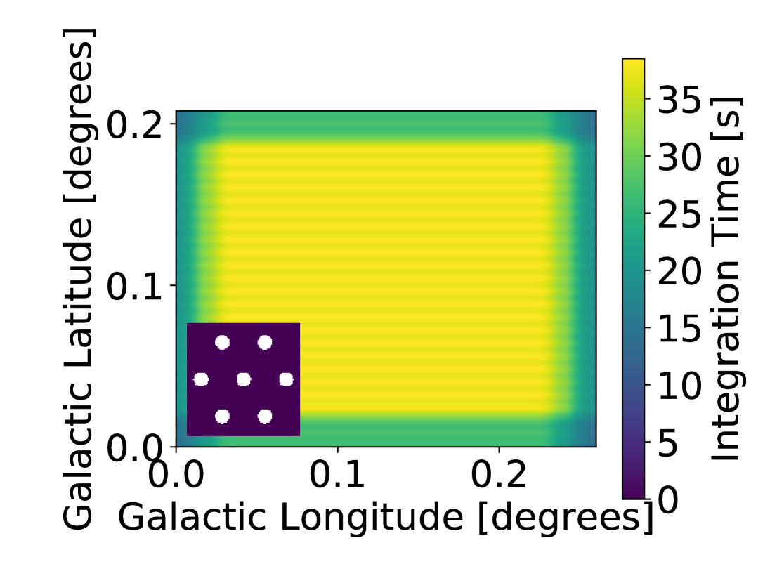
Figure 2: The color shows the expected integration time for each spectrum in a data cube assuming the use all seven beams and the KFPA configuration given in the box to the lower left. The angle of the KFPA here provides the least uniform sampling.

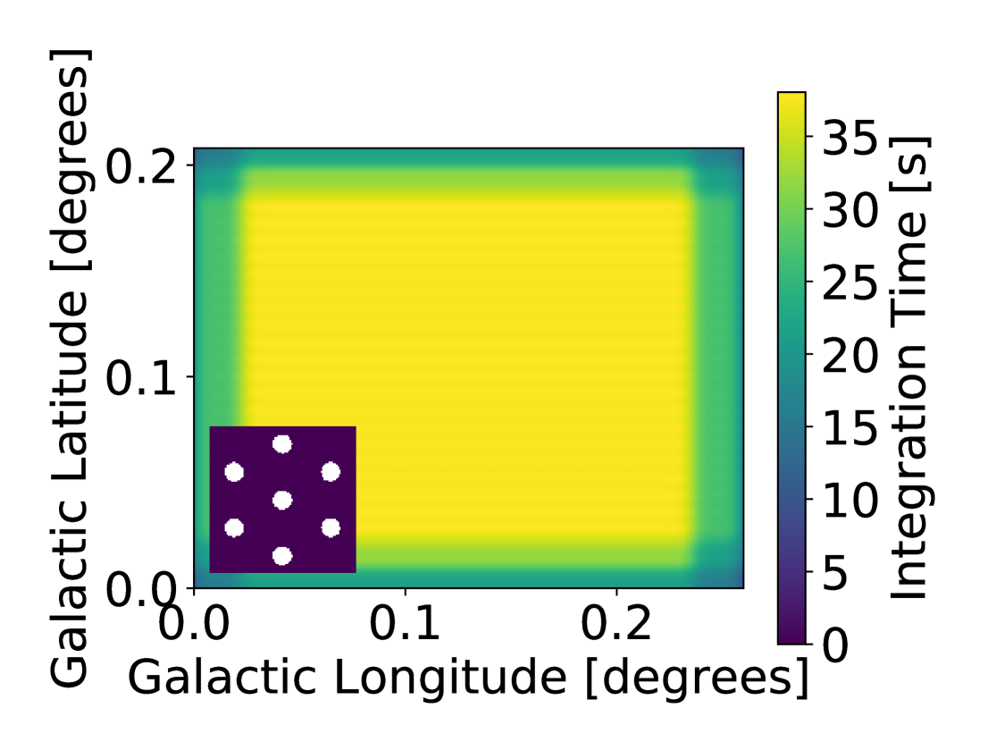
Figure 3: The color shows the expected integration time for each spectrum in a data cube assuming the use all seven beams and the KFPA configuration given in the box to the lower left. The angle of the KFPA here provides more uniform sampling than in Figure 2, but the sampling is still coarser in the Galactic latitude direction.

During the first 210 hr of GBT observing, RAMPS mapped approximately 6.5 square degrees in total for fields centered at $l=10^{\circ},23^{\circ},24^{\circ},28^{\circ},29^{\circ},30^{\circ},31^{\circ},38^{\circ},45^{\circ},\mathrm{and}\ 47^{\circ}$. Due to the success of the pilot survey and the legacy nature of the RAMPS dataset, RAMPS has been awarded additional observing time to extend the survey. Our goal is to map completely the 24 square degree survey region.

2.4 Data Reduction

We have reduced RAMPS data cubes in a standard manner using the GBT Mapping Pipeline (2011ASPC..442..127M) and the gbtgridder. The reduction process calibrates and grids the KFPA data to produce $l$,$b$,$v$ data cubes (i.e. an array of data with two spatial axes in Galactic coordinates, $l$ and $b$, and one velocity axis, $v$). The mapping pipeline calibrates and processes the raw data into FITS files for each array receiver, sub-band, and polarization, and the gbtgridder grids the spectra using a Gaussian kernel. We grid the data cubes with a pixel size of $6\arcsec$ and a channel width of $1.43\ \mathrm{kHz}\ (\sim 0.018\ \mathrm{km\ s^{-1}})$, where the central channel is at $V=0$ in the local standard of rest (LSR) frame. For each spectrum, the gbtgridder determines a zeroth-order baseline from the average of a group of channels near the edges of the band. It then generates a baseline-subtracted data cube that we use for further analysis.

2.5 Data Processing

We cropped the data cubes along both spatial and spectral axes. We performed the spatial cropping to remove pixels with no spectral data. We did this using PySpecKit (2011ascl.soft09001G), a Python spectral analysis and reduction toolkit. Specifically, we used the subcube function of the Cube class. We also cropped the data cubes on their spectral axis, and we did so for two reasons: to remove artifacts due to low gain at the edges of the passband, and to remove a portion of the $\mathrm{NH_{3}}$ spectra at large negative velocities. The edge of a spectrometer sub-band is less sensitive than at its center and can also exhibit a steep cusp if the baselines are not steady. We cropped all spectra by $\sim 3\%$ at each edge to remove this feature. After baseline fitting, we performed additional cropping on the $\mathrm{NH_{3}}$ spectra to remove unnecessary channels at large negative velocities. At the Galactic longitudes that RAMPS observes ($l=10^{\circ}-40^{\circ}$), CO source velocities range from $-60\ \mathrm{km\ s^{-1}}$ to $160\ \mathrm{km\ s^{-1}}$ (2001ApJ...547..792D). For the $\mathrm{NH_{3}}$ spectra, cropping the channels at velocities less than $-60\ \mathrm{km\ s^{-1}}$ should not remove real signal.

After cropping the edge channels, we regridded and combined adjacent cubes using the MIRIAD (STW95) tasks REGRID (version 1.17) and IMCOMB (version 1.11), respectively. This process resulted in data cubes of the L10, L23, 24, L28, L29, L30, and 31 fields, as well as portions of the L38, L45, and L47 fields. We also combined adjacent data cubes to create multifield maps of the L23-24 and L28-31 fields. Next, we applied a median filter to the spectra to increase signal-to-noise ratio (S/N), as well as to remove any anomalously large channel-to-channel variations. The original channel width of the RAMPS data cubes is $0.018\ \mathrm{km\ s^{-1}}$. We smoothed the $\mathrm{NH_{3}}$ data cubes along their spectral axis using a median filter with a width of 11 channels, which resulted in a new channel width of $0.2\ \mathrm{km\ s^{-1}}$. We chose this channel width to resolve in at least five spectral channels the typical line width found in high-mass SFRs (2016PASA...33...30R) and infrared dark clouds (2012ApJ...756...60S). We smoothed the $\mathrm{H_{2}O}$ data cubes using a median filter with a width of seven channels, which resulted in a new channel width of $0.12\ \mathrm{km\ s^{-1}}$. We smoothed the $\mathrm{H_{2}O}$ data with a smaller filter, in part because $\mathrm{H_{2}O}$ maser lines are generally bright and have larger S/Ns than the typical $\mathrm{NH_{3}}$ lines, as well as the need for higher spectral resolution to avoid blending multiple velocity components.

Next, we subtracted a polynomial baseline to remove any remaining passband shape. Before fitting for a baseline, we attempted to mask any spectral lines present in the spectra, since these would influence the baseline fit if left unmasked. To perform this masking in an automated manner, we masked groups of spectral channels that had a larger-than-average standard deviation, since these channels likely contained spectral lines. For each channel we calculated the standard deviation of the nearest 40 channels, which we will refer to as a channel’s $``$local standard deviation.” We then masked channels that had a local standard deviation larger than 1.5 times the median of the local standard deviations of all channels in the spectrum. Channels with a large local standard deviation were likely the result of a spectral line, while, on the other hand, a slowly varying baseline shape would result in channels with a smaller local standard deviation. This method reliably masked the majority of lines but was prone to miss broad-line wings. To mitigate this, we also masked channels that were within 10 channels of a masked channel. Next, we fit spectra for a polynomial baseline of up to second order, where the order is chosen such that the fit results in the smallest reduced $\chi^{2}$. We then subtracted the baseline function from the original spectrum and smoothed the baseline-subtracted spectrum as described above.

After subtracting a baseline, we attempted to test the quality of the fit in an automated manner. Our method involved comparing the true noise in a spectrum to the rms in the line-free regions of the spectrum. To estimate the true noise, we calculated the noise using the average channel-to-channel difference. We refer to the channel-to-channel noise as $\sigma_{\rm{diff}}$, where $\sigma_{\rm{diff}}=\sqrt{\frac{1}{2}\langle(T_{i}-T_{i+1})^{2}\rangle_{i}}$, where $T_{i}$ is the intensity of the $i^{th}$ channel and $\langle(T_{i}-T_{i+1})^{2}\rangle_{i}$ is the mean value of the square of the channel-to-channel differences. While the rms is influenced by both the true noise and any baseline present in the spectrum, $\sigma_{\rm{diff}}$ is relatively unaffected by the presence of both a signal and a baseline, as long as they are slowly varying compared to the channel spacing (2016PASA...33...30R). Thus, if the rms and $\sigma_{\rm{diff}}$ of the line-free portion of a spectrum are very different, there is likely a significant residual baseline present.

To test this, we simulated $10^{5}$ synthetic spectra with 15,384 channels, the size of unsmoothed RAMPS spectra after cropping. The synthetic spectra consisted of random Gaussian noise with a known standard deviation. We then smoothed the spectra with a median filter to match the real data since the $\mathrm{H_{2}O}$ data were smoothed with a seven-channel filter and the $\mathrm{NH_{3}}$ data were smoothed with an 11-channel filter. Next, we calculated the relative difference ($R$) between the rms and $\sigma_{\rm{diff}}$, given by $R=1-\frac{\sigma_{\rm{diff}}}{rms}$, for each synthetic spectrum. In Figure 4 we present two histograms of the distribution of $R$. The left panel shows the distribution of $R$ for the synthetic spectra smoothed with a filter width of seven channels, while right panel shows the distribution of $R$ for the synthetic spectra smoothed with a filter width of 11 channels. The two histograms have a mean of $\mu_{R}\sim 0$ and standard deviations of $\sigma_{R}\sim 0.01$ or $1\%$. Thus, $\sigma_{\rm{diff}}$ is a reliable estimator of the true rms for Gaussian noise. Next, we added a Gaussian signal to each synthetic spectrum to determine how $\sigma_{\rm{diff}}$ responds to the presence of signal. We gave the Gaussian signals uniform random values for both their line widths and S/Ns, where the line widths ranged from 0 to 10 channels and the S/Ns ranged from 0 to 100. For each synthetic spectrum of noise plus signal, we calculated $R$ and binned the values as a function of the amplitude and standard deviation of the synthetic signal, which is shown in Figure 5. Thus, $\sigma_{\rm{diff}}$ is also a reliable estimate of the noise when signal is present, except in spectra that contain very strong signals with relatively small line widths. This is not a problem for the $\mathrm{NH_{3}}$ data because the $\mathrm{NH_{3}}$ lines in the RAMPS dataset have S/N $<100$ and line widths of $\sigma>1$ channel. On the other hand, the $\mathrm{H_{2}O}$ masers in the RAMPS dataset can have S/N $>1000$ and line widths of $\sigma\sim 2$ channels, which adds a large source of error to $\sigma_{\rm{diff}}$. Hence, bright, narrow lines must be masked in order for $\sigma_{\rm{diff}}$ to accurately represent the true noise in a spectrum.

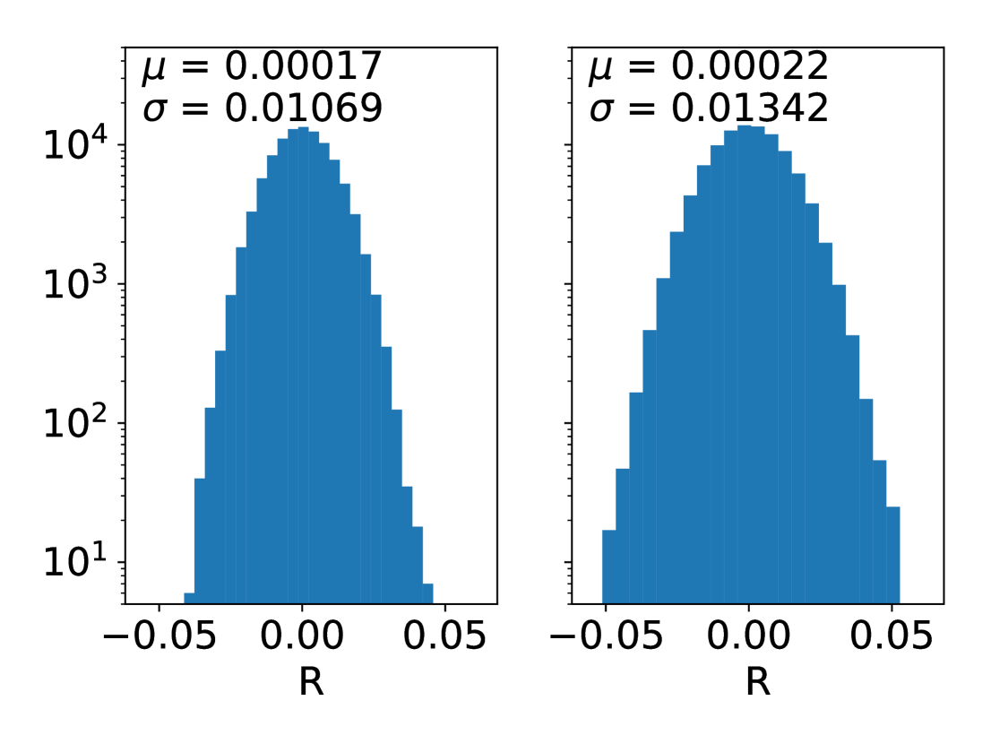
Figure 4: Histograms of the relative difference $R$ between the rms and $\sigma_{\rm{diff}}$ for $10^{5}$ synthetic spectra of Gaussian noise, where the relative difference is given by $R=1-\frac{\sigma_{\rm{diff}}}{rms}$. Our noise estimate is given by $\sigma_{\rm{diff}}=\sqrt{\frac{1}{2}\langle(T_{i}-T_{i+1})^{2}}\rangle_{i}$, where $T_{i}$ is the intensity of the $i^{\rm{th}}$ channel and $\langle(T_{i}-T_{i+1})^{2}\rangle_{i}$ is the mean of the square of all channel-to-channel differences. Listed in each panel are the mean ($\mu$) and standard deviation ($\sigma$) of each distribution. Left: distribution of $R$ for the synthetic spectra smoothed with a median filter width of seven channels. Right: distribution of $R$ for the synthetic spectra smoothed with a median filter width of 11 channels. Thus, for pure Gaussian noise, our noise estimate is a reliable estimator of the rms, with $\mu\sim 0$ and $\sigma\sim 0.01$ or 1%.

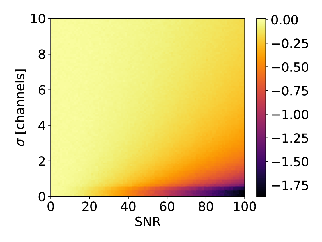
Figure 5: Color corresponds to the relative difference $R$ between the rms and $\sigma_{\rm{diff}}$ for $10^{5}$ synthetic spectra. We added synthetic Gaussian signals of varying width and amplitude and calculated $R=1-\frac{\sigma_{\rm{diff}}}{rms}$ for each spectrum. We binned the values of $R$ according to the line width $\sigma$ and the S/N to show the effect on $\sigma_{\rm{diff}}$ caused by the presence of signal. This analysis shows that only bright, narrow lines significantly affect the accuracy of $\sigma_{\rm{diff}}$.

Because bright lines add error to our estimate of the true noise, we masked each spectrum before comparing the rms to $\sigma_{\rm{diff}}$. As a first estimate of the true noise, we calculated $\sigma_{\rm{diff}}$ for the unmasked spectrum. We then masked channels with an intensity greater than $3\sigma_{\rm{diff}}$, as well as channels that were within 10 channels of a masked channel. Because bright $\mathrm{H_{2}O}$ masers add a large source of error to $\sigma_{\rm{diff}}$, we also measure $\sigma_{\rm{diff}}$ for the masked spectrum, which does not include very bright lines. We then used this new measurement of $\sigma_{\rm{diff}}$ to again mask channels with an intensity greater than $3\sigma_{\rm{diff}}$, as well as channels that were within 10 channels of a masked channel. We then calculated $R$ for this masked spectrum and used this value of $R$ to test the quality of the baseline fit. We also recorded the rms of the spectra, which we used as our estimate of the noise for later analysis. In Figure 6 we give a few examples of RAMPS $\mathrm{NH_{3}}$(1,1) spectra and their associated values of $R$, which show that a poor baseline fit generally results in a larger value of $R$. A poor baseline fit can occur for spectra in which the spectral mask did not exclude all of the signal, as well as for spectra with a baseline shape more complicated than second order. While our spectral mask was reliable for the majority of $\mathrm{NH_{3}}$ lines in the RAMPS dataset, some lines where broader than a typical $\mathrm{NH_{3}}$ line and were not well masked. To better fit spectra of this class, we attempted a second fit on spectra with $R>3\sigma_{R}$ using a slightly different mask. To mask broader lines more effectively, we employed the same masking technique as for the initial fit but this time used a 120-channel, rather than 40-channel, window to calculate the array of local standard deviations. Due to the larger window size, this mask was more sensitive to broader spectral features, and so it more successfully masked broad lines. We performed another baseline fit using this masked spectrum and once again calculated $R$. If the spectrum is well fit by the second fit, $R$ will likely be low, but if there is a residual baseline shape more complicated than second order, $R$ will still be large. Low-amplitude signal that was not well masked may also increase the measured value of $R$. In either case, a poor fit has the potential to alter line amplitude ratios, which would change the parameter values calculated from future fits to the data. To mitigate this potential problem, if a spectrum had $R>3\sigma_{R}$ after the second fit, we performed a third, more conservative fit. We used the mask from the second fit and forced a zeroth-order baseline fit, which is less likely to change the line amplitude ratios. In Figure 7, we show histograms of $R$ for all of the baseline fits of the $\mathrm{NH_{3}}$(1,1), $\mathrm{NH_{3}}$(2,2), and $\mathrm{H_{2}O}$ spectra. The distributions show a Gaussian component centered at $R\sim 0$, with long tails out to larger values of $R$. The Gaussian portions of each distribution match relatively well with the distributions found for synthetic Gaussian noise. The long tails in the distributions represent the poor baseline fits that were fit with a zeroth-order baseline. The vertical magenta line corresponds to $R=3\sigma_{R}$, which shows the approximate threshold between good and bad baselines expected from the analysis of the synthetic data. Significantly bad baselines are rare in this dataset, with the percent of spectra with $R>3\sigma_{R}$ for the $\mathrm{NH_{3}}$(1,1), $\mathrm{NH_{3}}$(2,2), and $\mathrm{H_{2}O}$ data equal to $3.1\%$, $2.4\%$, and $2.5\%$, respectively. While the majority of the data are of a high quality, there are spectra in the dataset that require higher-order baseline fitting and more careful masking than our automated techniques can provide. Because we intend to create a catalog of molecular clumps from the RAMPS dataset, we will look in more detail at each detected clump. For those clumps with poorly fit spectra, we will attempt another baseline fit with a more carefully chosen spectral mask and baseline polynomial order.

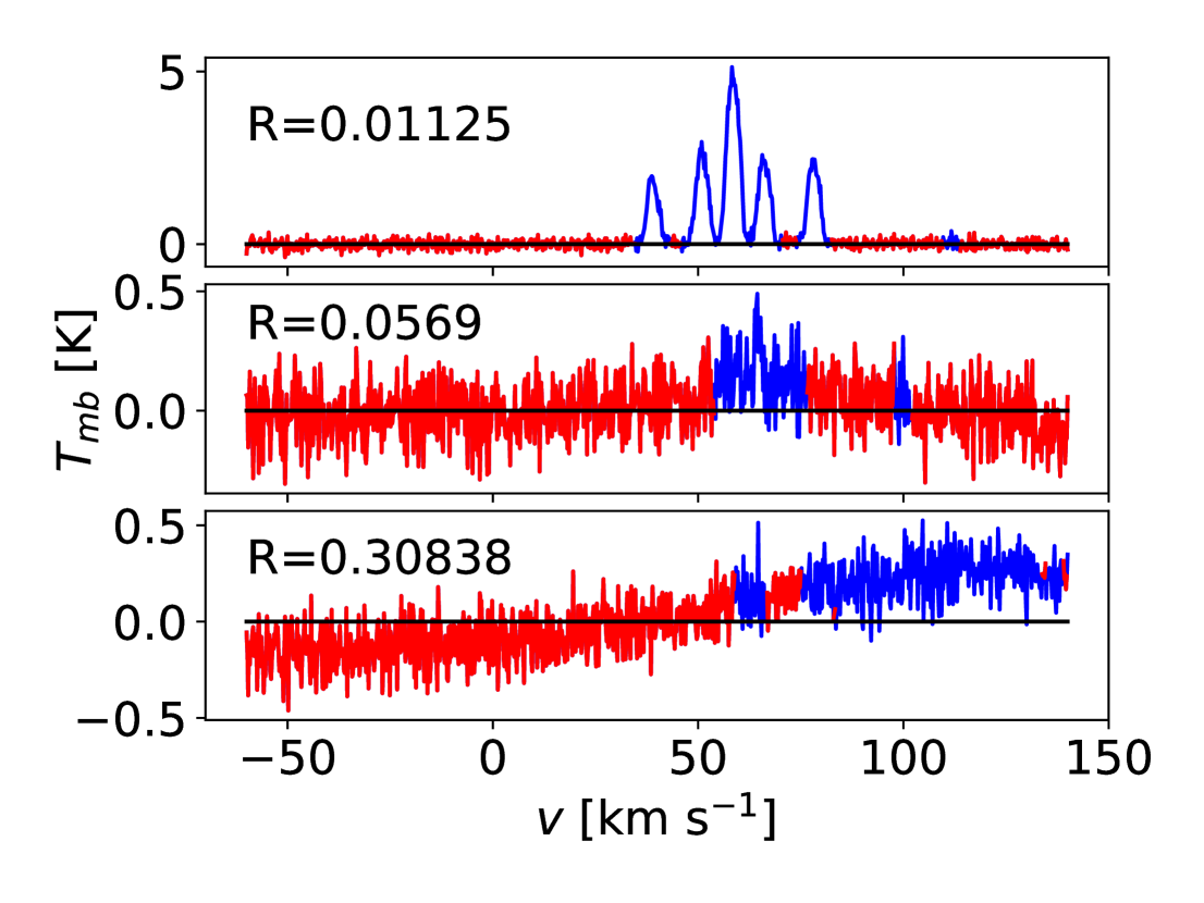
Figure 6: Examples of RAMPS $\mathrm{NH_{3}}$(1,1) spectra and their associated values of $R$. We fit spectra that have a large value of $R$ in a more conservative manner in order to preserve the line shape of any signal present. We show the full spectra in blue, overplot the masked spectra in red, and also show a fiducial line at $T_{mb}=0$ K. Top: this spectrum exhibits a bright $\mathrm{NH_{3}}$(1,1) line and shows little evidence for a residual baseline. The line is well masked, and consequently the spectrum has a low value of $R$. Middle: this spectrum exhibits a weak $\mathrm{NH_{3}}$(1,1) line and shows evidence for a moderate residual baseline. The weak line is relatively well masked, but the residual baseline results in a moderately high value for $R$. Bottom: this spectrum does not contain an obvious $\mathrm{NH_{3}}$(1,1) line but shows evidence for a significant residual baseline, resulting in a large value for $R$.

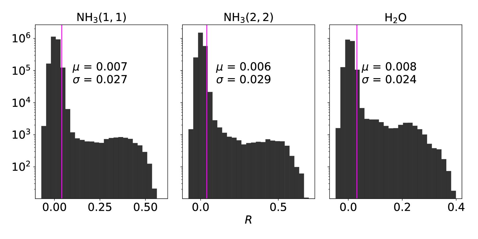
Figure 7: Histograms of $R$ for all RAMPS spectra, separated by line. The distributions each have a Gaussian component expected from the analysis of simulated spectra, but they also have a long tail to higher values of $R$, indicating poorly fit spectra. The magenta lines show the $R=3\sigma_{R}$ threshold used to restrict the complexity of the baseline fits.

We used the rms, calculated in the manner described above, as our estimate of the noise in a spectrum. This estimate includes a contribution from the true noise, as well as from any residual baseline that is present. After calculating the noise, we determined the integrated intensity and first moment of each spectrum. First, we masked each channel with a value less than five times the rms. If there was only one unmasked channel, we masked the entire spectrum. Otherwise, we summed over the unmasked channels to obtain the integrated intensity in units of $\mathrm{K\ km\ s^{-1}}$. Using the same spectral mask, we determined the first moment using the formula $\langle v\rangle=\frac{\Sigma v_{i}T_{i}}{\Sigma T_{i}}$, where $T_{i}$ and $v_{i}$ are the intensity and velocity of the $i^{th}$ channel, respectively.

2.6 Data Release

RAMPS data that are currently released to the public consist of $\mathrm{NH_{3}}$(1,1), $\mathrm{NH_{3}}$(2,2), and $\mathrm{H_{2}O}$ data cubes and their corresponding noise maps, as well as maps of $\mathrm{NH_{3}}$(1,1) and $\mathrm{NH_{3}}$(2,2) integrated intensity, $\mathrm{NH_{3}}$ velocity field, rotational temperature, total $\mathrm{NH_{3}}$ column density, $\mathrm{NH_{3}}$(1,1) optical depth, and $\mathrm{NH_{3}}$ line width. We present the integrated intensity and velocity field maps in Section 3 and the maps of rotational temperature, total $\mathrm{NH_{3}}$ column density, $\mathrm{NH_{3}}$ line width, and $\mathrm{H_{2}O}$ maser positions in Section LABEL:sec:analysis. RAMPS is an ongoing observing project, with the derived data being released annually upon verification. These data from the pilot survey are available at the RAMPS website (see footnote 1).

3 Results

Figure 8 shows three histograms of the noise in the smoothed RAMPS Pilot spectra, one histogram each for $\mathrm{NH_{3}}$(1,1), $\mathrm{NH_{3}}$(2,2), and $\mathrm{H_{2}O}$ $6_{1,6}-5_{2,3}$. Since we use seven receivers to observe the $\mathrm{NH_{3}}$ lines as compared to the single receiver we use to observe the $\mathrm{H_{2}O}$ maser line, the integration times per pixel are longer for the $\mathrm{NH_{3}}$ spectra. Thus, the $\mathrm{NH_{3}}$ spectra have much lower noise than the $\mathrm{H_{2}O}$ spectra. To show the spatial variations in the noise, we also present noise maps of all RAMPS fields observed during the pilot survey. Figures LABEL:fig:L10_11_noise$-$LABEL:fig:L47_11_noise show the $\mathrm{NH_{3}(1,1)}$ noise maps, Figures LABEL:fig:L10_22_noise$-$LABEL:fig:L47_22_noise show the $\mathrm{NH_{3}(2,2)}$ noise maps, and Figures LABEL:fig:L10_H2O_noise$-$LABEL:fig:L47_H2O_noise show the $\mathrm{H_{2}O}$ maser noise maps. Since spectra from tiles observed in poor weather or at low elevations have much higher noise, the noise often varies significantly from tile to tile. Although several tiles show significantly higher noise than the average noise within their fields, we intend to reobserve only those tiles that show evidence of emission in the BGPS maps, so as not to waste future observing time. There is also evidence for noise variations within tiles due to the nonuniform integration time across a tile (Figures 2 and 3), changes in weather or source elevation over the course of an observation, and the stitching together of partial observations of a single tile. As shown in Figures LABEL:fig:L10_11_noise-LABEL:fig:L47_H2O_noise, these variations are generally small, but they can be significant in certain tiles. For the rare circumstances where the noise variations within a tile are a significant detriment to our analysis of the data, we intend to reobserve.

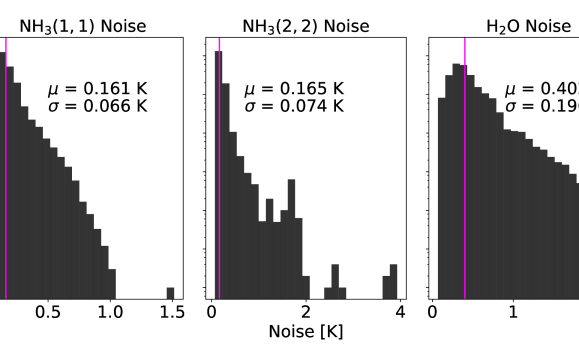
Figure 8: Histograms of the rms in each spectrum, separated by line. The mean value $\mu$ of each noise distribution is indicated by a magenta line and is printed on each plot along with the standard deviation $\sigma$ of each distribution.