Extracting many-body color charge correlators in the proton
from exclusive DIS at large Bjorken x

Abstract

We construct a general QCD light front formalism to compute many-body color charge correlators in the proton. These form factors can be extracted from deeply inelastic scattering measurements of exclusive final states in analogy to electromagnetic form factors extracted in elastic electron scattering experiments. Particularly noteworthy is the potential to extract a novel Odderon form factor, either indirectly from exclusive $J/\Psi$ measurements, or directly from exclusive measurements of the $\eta_{c}$ or tensor mesons at large Bjorken x. Besides the intrinsic information conveyed by these color charge correlators on the spatio-temporal tomography at the sub-femtoscopic scale at large x, the corresponding cumulants extend the domain of validity of McLerran-Venugopalan type weight functionals from small x and large nuclei to nucleons and light nuclei at large $x$, as well as to non-zero momentum transfer. This may significantly reduce nonperturbative systematic uncertainties in the initial conditions for QCD evolution equations at small $x$ and could be of strong relevance for the phenomenology of present and future collider experiments.

I Introduction

The increasing availability of high energies and high luminosities at fixed target and collider experiments Boer:2011fh ; Dudek:2012vr allows for unprecedented access to the internal transverse spatial and momentum distributions of color charge distributions inside nucleons and in nuclei. The standard framework Ji:2003ak is that of Wigner distributions Wigner:1932eb that allow simultaneous knowledge of both spatial and momentum aspects of the nucleon wave function. Knowledge of the Wigner distributions allows the construction of generalized parton distributions (GPDs) Mueller:1998fv ; Ji:1996ek ; Radyushkin:1996nd ; Collins:1996fb ; Diehl:2003ny ; Belitsky:2005qn ; Burkardt:2002hr and transverse momentum distributions (TMDs) Ralston:1979ys ; Collins:1981uk ; Mulders:1995dh ; Boer:1997nt ; Belitsky:2002sm ; Miller:2008sq that are generalizations of the usual collinear parton distributions. The GPDs provide information on the spatial tomography of the nucleon and TMDs allow for its momentum tomography.

These various distributions are very valuable. Our aim here is to introduce a complementary approach employing the Hamiltonian light front formalism in light cone gauge that allows essential insight into the dynamics of color charges in nucleons and nuclei. In this framework, color charge densities, and higher cumulants of these, can be defined and expressed as matrix elements of nonperturbative boost-invariant light front Fock-space wave functions of the QCD Hamiltonian. The corresponding form factors can be related to physical observables; these are the exclusive final states measured in deeply inelastic scattering (DIS) experiments. The information on color charge distributions extracted from such exclusive DIS measurements will be closely analogous to the information gathered on electric charge and magnetization distributions from form factors measured in elastic scattering of electrons by nucleons and nuclei Punjabi:2015bba ; Miller:2007uy ; Miller:2010nz ; Carlson:2007xd .

However because the QCD coupling $\alpha_{S}$ is much stronger than the QED fine structure constant, exclusive DIS experiments provide more information on color charge distributions, and higher cumulants of these, than elastic scattering experiments. Though it is true that GPDs and TMDs can be expressed in terms of light front wave functions Burkardt:2000za ; Dominguez:2011wm ; Petreska:2018cbf , our treatment in terms of color charge densities is novel.

The suite of feasible exclusive DIS final states is a rich source of information on many-body parton correlations with variations in $x_{\rm Bj}$ and $Q^{2}$ and can be expected to lead to an understanding of the internal spatial color charge structure of nucleons. The possible modification of this structure in nuclei, could be important for understanding the EMC effect in DIS and nucleon-nucleon short range correlations in nuclei Hen:2016kwk ; Miller:2015tjf . Also very intriguing is the possibility of comparing the color charge form factors to be discussed here with those that are now beginning to be extracted from lattice QCD computations Winter:2017bfs .

An attractive feature of the Hamiltonian light front framework is that the color charge form factors extracted in DIS can be employed to compute cross sections in hadron-hadron and hadron-nucleus scattering. The usefulness of such color charge form factors is known for QCD in the Regge limit of high energy scattering, with momentum resolution scales $Q^{2}\gg\Lambda_{\rm QCD}^{2}$ and $x_{\rm Bj}\sim Q^{2}/s\rightarrow 0$, with $s$ representing the squared center of mass energy in the experiment, as understood in the Color Glass Condensate (CGC) Iancu:2003xm ; Gelis:2010nm ; Kovchegov:2012mbw ; Blaizot:2016qgz . This is an effective field theory of the Regge limit of QCD that is formulated on the light front, with all the nontrivial information regarding multigluon correlations contained in a gauge invariant weight functional $W[\rho]$ that plays the role of a density matrix. Here, $\rho$ represents the color charge density of large $x$ partons coupled to small $x$ gluon fields.

This weight functional was first derived by McLerran and Venugopalan (MV) McLerran:1993ni ; McLerran:1993ka ; McLerran:1994vd , who also outlined the elements of the CGC EFT using light front arguments. They argued that for a large nucleus $A$, a probe of transverse size $\sim 1/Q$ couples coherently (for $x\ll A^{-1/3}$) along its path length to partons confined to nucleons in the nucleus. While on average, the probe sees no net color charge, the physics of random walks indicates that it will see large fluctuations of the color charge and therefore, by the central limit theorem, $W[\rho]$ will be Gaussian. These statements can be formulated with mathematical rigor Kovchegov:1996ty ; Jeon:2004rk .

The variance of the Gaussian, is the color charge squared per unit area $\mu_{\rm MV}^{2}\propto A^{1/3}$. In the large $A$ limit $\mu_{\rm MV}^{2}\gg\Lambda_{\rm QCD}^{2}$, so that the CGC is a weakly coupled EFT that allows for systematic computation of multigluon correlation functions that capture the physics underlying the phenomenon of gluon saturation Gribov:1984tu ; Mueller:1985wy in the high energy limit. The building block of gluon radiation, the Weizsäcker-Williams distribution, is screened at the scale $Q_{S}^{2}\propto\mu_{\rm MV}^{2}$ Ayala:1995kg ; JalilianMarian:1996xn ; Kovchegov:1996ty , and one recovers the phenomenologically successful Glauber-Mueller dipole model Mueller:1989st ; Mueller:1999wm of gluon saturation McLerran:1998nk ; Kovchegov:1999yj ; Venugopalan:1999wu .

The MV model does not describe the small $x$ evolution of the color source densities that arise from the $\alpha_{S}\ln(x)\sim O(1)$ enhanced bremsstrahlung of gluons. This is given by the JIMWLK equation that describes the functional renormalization group evolution of $W[\rho]$ with decreasing $x$  JalilianMarian:1997gr ; JalilianMarian:1997dw ; Iancu:2000hn ; Ferreiro:2001qy . This functional equation gives the Balitsky-JIMWLK hierarchy Balitsky:1995ub ; Weigert:2000gi . The equivalent functional Langevin equation was solved numerically Blaizot:2002np ; Rummukainen:2003ns . In the limit of large $N_{c}$, and large $A$, the lowest equation in this hierarchy, describing the $x$ evolution of “dipole” 2-point correlators of lightlike Wilson lines, has a closed form expression–the Balitsky-Kovchegov (BK) equation Balitsky:1995ub ; Kovchegov:1999yj , which reduces to the BFKL equation Kuraev:1977fs ; Balitsky:1978ic if the density of sources is sufficiently low.

Remarkably, as first conjectured in Iancu:2002aq , numerical simulations of the functional Langevin equation demonstrate that the hierarchy of correlators is to good approximation solved by a Gaussian $W[\rho]$ Dumitru:2011vk , with $\mu_{\rm MV}^{2}\longrightarrow\mu_{\rm JIMWLK}^{2}(x,k_{\perp})$, where $\mu_{\rm JIMWLK}^{2}(x,k_{\perp})$ is given by the solution of the BK equation. This Gaussian effective theory provides a quantitative phenomenology of electron-proton collisions at HERA Albacete:2010sy ; Kuokkanen:2011je ; Lappi:2013zma . Further, the formulation of the CGC EFT in the language of color source densities allows a first principles formulation of multiparticle production in QCD at small $x$ Gelis:2006yv ; Gelis:2006cr ; Gelis:2007kn ; Gelis:2008rw ; Gelis:2008ad ; Kovchegov:1998bi ; Dumitru:2001ux .

The initial conditions for BK/JIMWLK evolution are given by the MV model which, as noted, is formulated for large nuclei. Here we are concerned with the nucleon at large $x$. In this case, the central limit theorem is not applicable and the color charge form factors of the proton can reasonably be expected to be very different than in the MV model. Therefore a first principles computation of these form factors is in order. Such a computation is of intrinsic interest and can help constrain the systematic uncertainties in the QCD evolution of color charge distributions in the proton arising from the initial conditions. The spatial distributions of color charge density in the proton is also of great topical interest because of the unexpected long range azimuthally collimated “ridge” multiparticle correlations measured at RHIC and LHC Dusling:2015gta ; the latter may depend sensitively on the former Bjorken:2013boa ; Schenke:2014zha ; McLerran:2016snu ; Dusling:2018hsg ; Boer:2018vdi ; Kovchegov:2018jun ; Mace:2018vwq . Several models have been constructed to incorporate spatial nucleon color charge distributions in describing these data. However, they are constrained in varying degrees by systematic uncertainties in the initial conditions Mantysaari:2016ykx ; Bozek:2016kpf ; Albacete:2016pmp .

Here we develop a light front Hamiltonian framework that can be used to compute color charge form factors in nucleons and nuclei. The light front formalism we will employ is standard; see for instance Brodsky:1997de . We focus on the simple problem of constructing quadratic and cubic combinants of a three quark Fock state at large $x$. The color charge combinants can alternatively be expressed in terms of color charge form factors. We will discuss how information on these form factors can be cleanly extracted in exclusive DIS measurements of vector and tensor mesons at large $x$. An interesting possibility is the extraction of a novel Odderon color charge form factor in such measurements Lukaszuk:1973nt . As we will discuss, large $x$ DIS exclusive measurements should be particularly sensitive to the Odderon. This is of topical interest in light of recent claims that the TOTEM experiment may have found evidence of Odderon exchange in proton-proton elastic scattering at the highest LHC energies Antchev:2017yns .

This paper is organized as follows. In section 2, we begin by displaying the light front wavefunction for the proton, focusing immediately on the three valence quark component of the wavefunction. The extension to higher Fock states would be straightforward, but more involved. We also establish the notations and conventions to be employed in the rest of the paper. We then develop in section 3, in successive subsections, the general framework to compute light front color charge densities for the valence states, and the computation of the expectation values of quadratic and cubic color charge operators. In the last of these subsections, we compare our results to the MV model and demonstrate the relation between the gluon distribution in the proton and a quadratic correlator of color charge densities. The relation of the corresponding color charge form factors to exclusive heavy quark pair production in DIS is discussed in Section 4. In particular, we show that $J/\Psi$ production is sensitive to both a quadratic “Pomeron” color charge form factor and the cubic Odderon color charge form factor. In contrast, $\eta_{c}$ or tensor meson production are depends only on the Odderon form factor. In the concluding section, we will further discuss the prospects of Odderon discovery in DIS experiments in light of prior searches. We will also discuss more generally the prospects for quantitative constraints on the quadratic and cubic color charge form factors from DIS data at large $x_{\rm Bj}$. We shall also outline the next steps both on further theoretical development of this framework and in quantitative comparison and predictions for measurements at extant and future experiments. The paper contains two appendices. In Appendix A, we discuss the color charge density operator in the limit of large longitudinal momenta. In Appendix B, we provide some details of the computation of the Odderon form factor.

II The light front proton wavefunction: notation and conventions

In this section, we shall introduce our notation and conventions for the proton wavefunction on the light front. These closely follow Refs. Brodsky:1989pv ; Brodsky:2000ii . The light front wavefunction of an unpolarized on-shell proton with four-momentum $P^{\mu}=(P^{+},P^{-},\vec{P}_{\perp})$ can be expressed as

$$|P\rangle=\int{\rm d}\mathrm{PS}_{n}\sum_{n}\psi_{n}|n\rangle~{}\,,$$ (1)

where $|n\rangle$ are the Fock space basis vectors of the light front Hamiltonian, $\psi_{n}=\langle n|P\rangle$ is the amplitude for a particular Fock state $|n\rangle$ in the proton and ${\rm d}\mathrm{PS}$ denotes the $n$-body phase space for $|n\rangle$. If the proton light front wavefunction is dominated by its valence quark state, as is the case at large values of Bjorken $x$, it is given explicitly as

$$|P\rangle = \frac{1}{\sqrt{6}}\int\frac{{\rm d}x_{1}{\rm d}x_{2}{\rm d}x_{3}}{\sqrt{x_{1}x_{2}x_{3}}}\delta(1-x_{1}-x_{2}-x_{3})\int\frac{{\rm d}^{2}k_{1}{\rm d}^{2}k_{2}{\rm d}^{2}k_{3}}{(16\pi^{3})^{3}}16\pi^{3}\delta(\vec{k}_{1}+\vec{k}_{2}+\vec{k}_{3})$$ (2)

$$\times \sum_{\lambda_{1},\lambda_{2},\lambda_{3}}\psi_{3}(p_{1},\lambda_{1},p_{2},\lambda_{2},p_{3},\lambda_{3})\sum_{i_{1},i_{2},i_{3}}\epsilon_{i_{1}i_{2}i_{3}}|p_{1},i_{1},\lambda_{1};\,p_{2},i_{2},\lambda_{2};\,p_{3},i_{3},\lambda_{3}\rangle~{}.$$

The three on-shell quark momenta are specified by their lightcone momenta $p_{i}^{+}=x_{i}P^{+}$ and their transverse momenta $\vec{p}_{i}=x_{i}\vec{P}_{\perp}+\vec{k}_{i}$. Hence the $\vec{k}_{i}$ can be interpreted as the transverse momenta of the valence quarks relative to the proton. In addition to color, denoted by $i_{i}$, the quark Fock state also carries flavor and helicity quantum numbers which are collectively denoted as $\lambda_{i}$. The valence Fock state wave function in color space belongs to the product space obtained from the direct product of three triplet color spaces: $|i_{1};i_{2};i_{3}\rangle=|i_{1}\rangle\otimes|i_{2}\rangle\otimes|i_{3}\rangle$. The Levi-Civita tensor in Eq. (2) projects the product of three fundamental representations onto the totally anti-symmetric SU(3) singlet; a SU(3) transformation $U$ of $\epsilon_{i_{1}i_{2}i_{3}}|i_{1}\rangle|i_{2}\rangle i_{3}\rangle$ gives

$$\epsilon_{i_{1}i_{2}i_{3}}U_{j_{1}i_{1}}U_{j_{2}i_{2}}U_{j_{3}i_{3}}|j_{1}\rangle|j_{2}\rangle|j_{3}\rangle=\epsilon_{j_{1}j_{2}j_{3}}(\mathrm{det~{}}U)|j_{1}\rangle|j_{2}\rangle|j_{3}\rangle~{},$$ (3)

where det $U=1$ for $U\in$ SU(3).

The amplitude $\psi_{3}$ in Eq. (2) is symmetric under exchange of any two of its arguments and is normalized according to

$$\int{{\rm d}x_{1}{\rm d}x_{2}{\rm d}x_{3}}\,\delta(1-x_{1}-x_{2}-x_{3})\int\frac{{{\rm d}^{2}k_{1}{\rm d}^{2}k_{2}{\rm d}^{2}k_{3}}}{(16\pi^{3})^{3}}(16\pi^{3})\,\delta(\vec{k}_{1}+\vec{k}_{2}+\vec{k}_{3})\,\sum_{\lambda_{1},\lambda_{2},\lambda_{3}}|\psi_{3}|^{2}=1~{}.$$ (4)

Note that $\psi_{3}$ vanishes when the set $\{\lambda_{1},\lambda_{2},\lambda_{3}\}$ does not match the corresponding quantum numbers of the proton. The normalization of $\psi_{3}$ corresponds to the proton wavefunction normalization,

$$\langle K|P\rangle = 16\pi^{3}\,P^{+}\delta(P^{+}-K^{+})\,\delta(\vec{P}_{\perp}-\vec{K}_{\perp})$$ (5)

$$= 16\pi^{3}\,\delta(\Delta x)\,\delta(\vec{P}_{\perp}-\vec{K}_{\perp})~{}.$$ (6)

For simplicity, throughout the manuscript we take the fractional plus momentum transfer $\Delta x=(K^{+}-P^{+})/P^{+}$ to be very small or zero.

The one-particle quark states introduced above are created by the action of the quark creation operator $b^{\dagger}_{p,i,\lambda}$ on the one-particle vacuum $|0\rangle$:

$$|p,i,\lambda\rangle=b^{\dagger}_{p,i,\lambda}|0\rangle~{}.$$ (7)

Its Hermitian conjugate transforms an occupied one-particle state to the light front vacuum state,

$$b_{k,j,\sigma}|p,i,\lambda\rangle = \delta^{ji}\delta^{\sigma\lambda}\,k^{+}\delta(k^{+}-p^{+})\,16\pi^{3}\delta(\vec{k}-\vec{p})|0\rangle\equiv\delta_{k,p}^{ji,\sigma\lambda}\,|0\rangle~{},$$ (8)

$$b_{k,j,\sigma}|0\rangle = 0~{}.$$ (9)

In Eq. (8), we introduced a short hand notation $\delta_{k,p}^{ji,\sigma\lambda}\,$, which we will frequently use throughout the rest of the paper. We shall further also use the shorthand notation,

$$\delta_{k,p}^{ij}\, \equiv \delta^{ji}\,\delta_{k,p}\,\,$$ (10)

$$\delta_{k,p}\, \equiv k^{+}\delta(k^{+}-p^{+})\,16\pi^{3}\delta(\vec{k}-\vec{p})~{}.$$ (11)

The quark creation and destruction operators satisfy the anti-commutation relation,

$$\{b_{k,j,\sigma},b^{\dagger}_{p,i,\lambda}\}=\delta_{k,p}^{ji,\sigma\lambda}\,~{}.$$ (12)

These relations, along with the convention that $\langle 0|0\rangle=1$, determine the normalization of one-particle states as

$$\langle k,j,\sigma|p,i,\lambda\rangle=\langle 0|b_{k,j,\sigma}\,b^{\dagger}_{p,i,\lambda}|0\rangle=\langle 0|\{b_{k,j,\sigma},b^{\dagger}_{p,i,\lambda}\}|0\rangle=\delta_{k,p}^{ji,\sigma\lambda}\,~{}.$$ (13)

Furthermore,

$$\langle k,j,\sigma|b^{\dagger}_{q,m,\sigma^{\prime}}b_{r,n,\lambda^{\prime}}|p,i,\lambda\rangle=\delta_{k,q}^{jm,\sigma\sigma^{\prime}}\,\,\delta_{r,p}^{ni,\lambda\lambda^{\prime}}\,~{},$$ (14)

and

$$\langle k,j,\sigma|b_{q,m,\sigma^{\prime}}b^{\dagger}_{r,n,\lambda^{\prime}}|p,i,\lambda\rangle=\delta_{q,r}^{mn,\sigma^{\prime}\lambda^{\prime}}\,\delta_{k,p}^{ji,\sigma\lambda}\,-\delta_{k,r}^{jn,\sigma\lambda^{\prime}}\,\,\delta_{q,p}^{mi,\sigma^{\prime}\lambda}\,~{}.$$ (15)

With these relations in hand, one can derive matrix elements of density operators and powers thereof.

Before we discuss color charge densities, let us first consider the following operator:

$$\left[{\tilde{\rho}}^{mn}_{q}\right]_{1}=\int\limits_{\ell,\lambda}\!\!\!\!\!\!\!\!\!\sum\,b^{\dagger}_{\ell-q,m,\lambda}b_{\ell,n,\lambda}~{}.$$ (16)

We have written the integration measure here compactly as

$$\int\limits_{\ell,\lambda}\!\!\!\!\!\!\!\!\!\sum\equiv\int\limits_{0}^{\infty}\frac{{\rm d}\ell^{+}}{\ell^{+}}\int\frac{{\rm d}^{2}\ell}{16\pi^{3}}\sum_{\lambda}~{}~{}~{}~{},~{}~{}~{}~{}\int\limits_{\ell,\lambda}\!\!\!\!\!\!\!\!\!\sum\delta_{q,l}^{ij,\sigma\lambda}\,=\delta^{ij}~{}.$$ (17)

Setting $\vec{P}_{\perp}=0$ in the incoming proton for simplicity, and employing Eq. (14) and Eq. (12), we obtain the expectation value of the operator defined in Eq. (16) as

$$\langle K|\left[{\tilde{\rho}}^{mn}_{q}\right]_{1}|P\rangle = \frac{1}{16\pi^{3}}\delta^{mn}\int\frac{{\rm d}x_{1}{\rm d}x_{2}{\rm d}x_{3}}{\sqrt{x_{1}x_{2}x_{3}}}\delta(1-x_{1}-x_{2}-x_{3})\int{{\rm d}^{2}p_{1}{\rm d}^{2}p_{2}{\rm d}^{2}p_{3}}\,\delta(\vec{p}_{1}+\vec{p}_{2}+\vec{p}_{3})$$ (18)

$$\times \int\frac{{\rm d}y_{1}{\rm d}y_{2}{\rm d}y_{3}}{\sqrt{y_{1}y_{2}y_{3}}}\delta(1-y_{1}-y_{2}-y_{3})\int{{\rm d}^{2}k_{1}{\rm d}^{2}k_{2}{\rm d}^{2}k_{3}}\,\delta(\vec{k}_{1}+\vec{k}_{2}+\vec{k}_{3})$$

$$\times \sum_{\lambda_{1},\lambda_{2},\lambda_{3}}\psi_{3}^{*}(k_{1},k_{2},k_{3})\,\psi_{3}(p_{1},p_{2},p_{3})\,\delta_{k_{1},p_{1}-q}\,\delta_{k_{2},p_{2}}\,\delta_{k_{3},p_{3}}\,~{}.$$

It is implied that $y_{i}$, $\vec{k}_{i}$ are the momentum fractions and transverse momenta, respectively, of the quarks in the outgoing proton. However, there is a subtlety: the plus momenta of the quarks in the outgoing proton correspond to $k_{i}^{+}=y_{i}K^{+}=y_{i}(1+\Delta x)P^{+}$ rather than to $k_{i}^{+}=y_{i}P^{+}$. Therefore, in the arguments of the delta-functions originating from the Fock space matrix elements (the last three in the expression above) we have to shift $y_{i}\to y_{i}(1+\Delta x)$; we also have to shift $\vec{k}_{i}\to\vec{k}_{i}+y_{i}\vec{K}_{\perp}$ since there is a non-zero transfer of transverse momentum. To simplify the final expression we shall take $\Delta x\to 0$ so that

$$\langle K|\left[{\tilde{\rho}}^{mn}_{q}\right]_{1}|P\rangle = {16\pi^{3}}\delta(\vec{q}+\vec{K}_{\perp})\,\delta(x_{q}+\Delta x)\delta^{mn}\,$$ (19)

$$\times \int{\rm d}x_{1}{\rm d}x_{2}{\rm d}x_{3}\,\delta(1-x_{1}-x_{2}-x_{3})\int{{\rm d}^{2}p_{1}{\rm d}^{2}p_{2}{\rm d}^{2}p_{3}\over(16\pi^{3})^{2}}\,\delta(\vec{p}_{1}+\vec{p}_{2}+\vec{p}_{3})$$

$$\times \sum_{\lambda_{1},\lambda_{2},\lambda_{3}}\psi_{3}^{*}(k_{1},k_{2},k_{3})\,\psi_{3}(p_{1},p_{2},p_{3})~{}.$$

In the limit $\Delta x\to 0$ the arguments of $\psi_{3}^{*}$ are $k_{i}^{+}\simeq x_{i}P^{+}$, $\vec{k}_{1}\simeq\vec{p}_{1}+(1-x_{1})\vec{K}_{\perp}$, $\vec{k}_{2}\simeq\vec{p}_{2}-x_{2}\vec{K}_{\perp}$, $\vec{k}_{3}\simeq\vec{p}_{3}-x_{3}\vec{K}_{\perp}$. (Note that the flavor and helicity of each quark remains unchanged.)

The prefactor, ${16\pi^{3}}\delta(\vec{q}+\vec{K}_{\perp})\,\delta(x_{q}+\Delta x)$, of Eq. (19) is the overlap $\langle K|P\rangle$. This factor enters in the matrix elements that we compute, but according to the usual Feynman rules do not appear in the final invariant amplitudes. The remaining factors are $\delta^{mn}$ and a dimensionless matter ($M$) form factor, $F_{M}(q)$:

$$F_{M}(q)\equiv\int{\rm d}x_{1}{\rm d}x_{2}{\rm d}x_{3}\,\delta(1-x_{1}-x_{2}-x_{3})\int{{\rm d}^{2}p_{1}{\rm d}^{2}p_{2}{\rm d}^{2}p_{3}\over(16\pi^{3})^{2}}\,\delta(\vec{p}_{1}+\vec{p}_{2}+\vec{p}_{3})\sum_{\lambda_{i}}\psi_{3}^{*}(k_{1},k_{2},k_{3})\,\psi_{3}(p_{1},p_{2},p_{3})~{}.$$ (20)

If the transverse momentum transfer $\vec{K}_{\perp}$ is also much smaller than the typical momenta of the quarks in the proton, the remaining integral is proportional to the normalization integral for $\psi_{3}$ given in Eq. (4). In that case,

$$\langle K|\left[{\tilde{\rho}}^{mn}_{q}\right]_{1}|P\rangle\simeq 16\pi^{3}\,\delta^{mn}\,\delta(\vec{q}+\vec{K}_{\perp})\,\delta(x_{q}+\Delta x)~{}.$$ (21)

Indeed, stripping off the color space identity matrix and setting both $x_{q}$ and $\vec{q}$ to zero leads back to the normalization condition in Eq. (6) for the proton wavefunction.

III Light front expectation values of color charge densities and form factors

After the prior discussion of the essential preliminaries, we have all the elements in place to construct the light front color charge operator and expectation values of moments of expectation values of this operator in the large $x$ kinematic region where valence quarks dominate. We will later discuss the relation of these correlators to cross-sections for exclusive DIS final states.

III.1 The color charge density operator

The color charge current density associated with $f=1\dots N_{f}$ fermion fields $\psi_{f}$ is $j^{\mu a}=\bar{\psi}_{i,f}\gamma^{\mu}\psi_{j,f}(t^{a})_{ij}$. Here, $t^{a}$, $a=1\dots 8$ are the generators of the fundamental representation of color-SU(3) normalized as $\mathrm{tr\,}t^{a}t^{b}=\delta^{ab}/2$. They are hermitian and traceless, $\mathrm{tr\,}t^{a}=0$.

The quark creation and annihilation operators are defined from the Fourier mode expansion of the free field operator at light cone time $x^{+}=t+z=0$. Since we are focused here on valence quark color charge distributions, we ignore antiquark contributions to write (see Appendix II in Brodsky:1989pv ),

$$\psi_{i,f}(r)=\int{{\rm d}p^{+}{\rm d}^{2}p\over{16\pi^{3}p^{+}}}\,\sum_{s}b_{p,i,s,f}\,u^{s}(p)\,e^{-ip\cdot r}=\int{{\rm d}x_{p}{\rm d}^{2}p\over{16\pi^{3}x_{p}}}\,\sum_{s}b_{p,i,s,f}\,u^{s}(p)\,e^{-ip\cdot r}~{},$$ (22)

where $r\equiv(x^{+}=0,x^{-},\vec{x}_{\perp})$ is the coordinate vector. We wrote out spin and flavor indices explicitly in Eq. (22) and introduced the momentum fraction $x_{p}=p^{+}/P^{+}$. The integration over $p^{+}$ or $x_{p}$ is restricted to positive values. Using $\bar{u}_{k}\gamma^{+}u_{p}=2\sqrt{k^{+}p^{+}}$ we can then write the color charge density operator $\rho^{a}\equiv j^{+a}$ as

$$\rho^{a}(r)=2P^{+}\sum_{\lambda,\lambda^{\prime}}\int{{\rm d}x_{q}{\rm d}^{2}q\over{16\pi^{3}\sqrt{x_{q}}}}\,b^{\dagger}_{q,i,\lambda}e^{iq\cdot r}\int{{\rm d}x_{p}{\rm d}^{2}p\over{16\pi^{3}\sqrt{x_{p}}}}\,b_{p,j,\lambda^{\prime}}e^{-ip\cdot r}\,(t^{a})_{ij}\,\delta_{\lambda\lambda^{\prime}}~{}.$$ (23)

Note that here $b^{\dagger}b$ is diagonal in spin and flavor, collectively denoted here by $\lambda$. Performing a three-dimensional Fourier transform with respect to $x^{-}$ and $\vec{x}$, we obtain the color charge density operator in momentum space,

$${\tilde{\rho}}^{a}(x_{k},\vec{k})=\sum_{\lambda}\int\limits{{\rm d}x_{q}\over\sqrt{x_{q}(x_{q}+x_{k})}}\int\frac{{\rm d}^{2}q}{16\pi^{3}}\,b^{\dagger}_{q,i,\lambda}b_{k+q,j,\lambda}\,(t^{a})_{ij}~{}.$$ (24)

In this expression, there is a shift of the argument of the annihilation operator by $(k^{+},\vec{k})=(x_{k}P^{+},\vec{k})$ relative to the quark creation operator. The physical interpretation of $x_{k}$ is that it is the longitudinal momentum shift of the quark momentum following an interaction with a colored probe. In the high energy limit, where $P^{+}$ is large, the $x_{k}$ dependent corrections are of order $1/P^{+}$ and can be ignored. This is explained in Appendix A, where we show that the density is confined to a thin pancake in $x^{-}$, with support $1/P^{+}$. Thus to leading power in $P^{+}$, we approximate (in the notation of Eq. (17)) ${\tilde{\rho}}^{a}(x_{k}\to 0,\vec{k})\equiv{\tilde{\rho}}^{a}(\vec{k})$ so that

$${\tilde{\rho}}^{a}(\vec{k})=\int\limits_{q,\lambda}\!\!\!\!\!\!\!\!\!\sum b^{\dagger}_{x_{q},\vec{q},i,\lambda}\,b_{x_{q},\vec{k}+\vec{q},j,\lambda}\,(t^{a})_{ij}=\int\limits_{q,\lambda}\!\!\!\!\!\!\!\!\!\sum b^{\dagger}_{x_{q},\vec{q}-\vec{k},i,\lambda}\,b_{x_{q},\vec{q},j,\lambda}\,(t^{a})_{ij}~{}.$$ (25)

The operator in Eq. (25) differs from that in Eq. (16) because there is no shift in the longitudinal momentum. We use this expression in the remainder of this paper. Note the variables $(x_{q},\vec{q})$ are integrated over, so that the left-hand-side depends only on $\vec{k}$.

The color charge density per unit transverse area, given by the two-dimensional Fourier transform of this expression, is

$$\rho^{a}(\vec{x}_{\perp})=\int\frac{{\rm d}^{2}k}{(2\pi)^{2}}\,e^{i\vec{k}\cdot\vec{x}_{\perp}}\int\limits_{q,\lambda}\!\!\!\!\!\!\!\!\!\sum\,b^{\dagger}_{x_{q},\vec{q}-\vec{k},i,\lambda}\,b_{x_{q},\vec{q},j,\lambda}\,(t^{a})_{ij}~{}.$$ (26)

In the following subsections, and in the rest of the paper, we will employ an expectation value defined as

$$\langle{\bf O}\,\rangle_{K_{\perp}}=\frac{\Bigl{<}P^{+},\vec{K}_{\perp}\Bigl{|}\,{\bf O}\,\Bigr{|}P^{+},\vec{P}_{\perp}=0\Bigr{>}}{\langle K|P\rangle}\,,$$ (27)

where ${\bf O}$ denotes a generic operator constituted of products of $\rho^{a}(\vec{x}_{\perp})$ defined above, or its two-dimensional Fourier transform ${\tilde{\rho}}^{a}(\vec{k})$ in Eq. (25). The overlap $\langle K|P\rangle$ in Eq. (6) is the standard one given by

$$\langle K|P\rangle=16\pi^{3}\,P^{+}\,\delta(K^{+}-P^{+})\,\delta(\vec{K}_{\perp}-\vec{P}_{\perp})\,.$$ (28)

We shall be interested in the case when $K^{+}=P^{+}$ (see Appendix A).

III.2 $\langle\rho^{a}\rangle$ in the proton

The proton matrix element of the color charge density operator Eq. (25) is given by

$$\langle\,{\tilde{\rho}}^{a}(\vec{q})\,\rangle_{K_{\perp}} = \,\mathrm{tr\,}t^{a}\,\sum_{\lambda_{i}}\int{\rm d}x_{1}{\rm d}x_{2}{\rm d}x_{3}\,\delta(1-x_{1}-x_{2}-x_{3})$$ (29)

$$\times \int\frac{{\rm d}^{2}p_{1}{\rm d}^{2}p_{2}{\rm d}^{2}p_{3}}{(16\pi^{3})^{2}}\,\delta(\vec{p}_{1}+\vec{p}_{2}+\vec{p}_{3})\,\psi_{3}^{*}(k_{1},k_{2},k_{3})\,\psi_{3}(p_{1},p_{2},p_{3})~{}.$$

Recall that the arguments of $\psi_{3}^{*}$ are given by $k_{i}^{+}=p_{i}^{+}\equiv x_{i}P^{+}$, $\vec{k}_{1}=\vec{p}_{1}+(1-x_{1})\vec{K}_{\perp}$, $\vec{k}_{2}=\vec{p}_{2}-x_{2}\vec{K}_{\perp}$, $\vec{k}_{3}=\vec{p}_{3}-x_{3}\vec{K}_{\perp}$.

Since $\mathrm{tr\,}t^{a}=0$, the above expression is of course zero, as it should be in QCD. Before we move on to consider higher moments of the charge charge operator, which are non-zero, it is amusing to consider what charge conjugation does to the above expression. $C\,{\tilde{\rho}}^{a}(k)\,C^{-1}$ is given by an expression similar to Eq. (25) with the replacement $t^{a}\to-(t^{a})^{T}=-(t^{a})^{*}$. Therefore,

$$\langle\,C{\tilde{\rho}}^{a}(\vec{q})\,C^{-1}\,\rangle_{K_{\perp}} = -\,\left(\mathrm{tr\,}t^{a}\right)^{*}\,\sum_{\lambda_{i}}\int{\rm d}x_{1}{\rm d}x_{2}{\rm d}x_{3}\,\delta(1-x_{1}-x_{2}-x_{3})$$ (30)

$$\times \int\frac{{\rm d}^{2}p_{1}{\rm d}^{2}p_{2}{\rm d}^{2}p_{3}}{(16\pi^{3})^{2}}\,\delta(\vec{p}_{1}+\vec{p}_{2}+\vec{p}_{3})\,\psi_{3}^{*}(k_{1},k_{2},k_{3})\,\psi_{3}(p_{1},p_{2},p_{3})~{}.$$

III.3 $\langle\rho^{a}\rho^{b}\rangle$ in the proton

We shall now compute the first nontrivial color charge correlator, the expectation value of ${\tilde{\rho}}^{a}(q)\,{\tilde{\rho}}^{b}(k)$ in the proton. The contributions to its expectation value can be classified, as is common in many-body physics, into one-body and two-body contributions–these are illustrated in Fig. 1.

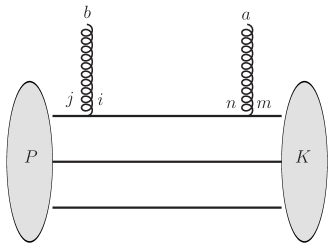
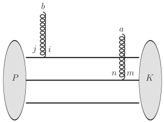
Figure 1: Illustration of the terms we call one-body (left figure) and two-body (right figure) contribution to the $\langle\rho^{a}\rho^{b}\rangle$ correlator. $i,j,n,m=1,2,3$ denote the colors of the quarks while $a,b=1\dots 8$ are those of the gluons that couple to them.

We begin with the one-body contribution, where both operators act on the same quark,

$$\left[{\tilde{\rho}}^{a}(q)\,{\tilde{\rho}}^{b}(k)\right]_{1}={\tilde{\rho}}^{a}(q)\,{\tilde{\rho}}^{b}(k)\otimes 1\!\!1\otimes 1\!\!1+\text{permutations}~{}.$$ (31)

Then using the anti-commutation relation Eq. (12), and keeping only the one-body contribution leads to:

$$b^{\dagger}_{x_{\ell_{1}},\vec{\ell}_{1}-\vec{q},i,\lambda}\,b_{x_{\ell_{1}},\vec{\ell}_{1},j,\lambda}b^{\dagger}_{x_{\ell_{2}},\vec{\ell}_{2}-\vec{k},m,\lambda^{\prime}}\,b_{x_{\ell_{2}},\vec{\ell}_{2},n,\lambda^{\prime}}\to\delta_{\ell_{1},\ell_{2}-k}^{jm,\lambda\lambda^{\prime}}\,\,b^{\dagger}_{x_{\ell_{1}},\vec{\ell}_{1}-\vec{q},i,\lambda}\,b_{x_{\ell_{2}},\vec{\ell}_{2},n,\lambda^{\prime}}~{},$$ (32)

and further, using the matrix element of $b^{\dagger}b$ given previously in Eq. (14), we get

$$\epsilon_{i_{1}i_{2}i_{3}}\epsilon_{j_{1}j_{2}j_{3}}\Bigl{<}p_{1}^{\prime},i_{1},\lambda_{1}^{\prime};p_{2}^{\prime},i_{2},\lambda_{2}^{\prime};p_{3}^{\prime},i_{3},\lambda_{3}^{\prime}\Bigl{|}\left[{\tilde{\rho}}^{a}(q)\,{\tilde{\rho}}^{b}(k)\right]_{1}\Bigr{|}p_{1},j_{1},\lambda_{1};p_{2},j_{2},\lambda_{2};p_{3},j_{3},\lambda_{3}\Bigr{>} =$$ (33)

$$3\delta^{ab}\delta_{p_{1}^{\prime},p_{1}-q-k}^{\lambda_{1}\lambda_{1}^{\prime}}\,\delta_{p_{2}^{\prime},p_{2}}^{\lambda_{2}\lambda_{2}^{\prime}}\,\delta_{p_{3}^{\prime},p_{3}}^{\lambda_{3}\lambda_{3}^{\prime}}\,\,.$$

The symmetry of $\psi_{3}$ under permutations has been used.

We will next compute the two-body contributions to the second moment of the color charge density, where one of the color charge density operators acts on one quark and the other acts on another quark, as illustrated in Fig. 1. Note that the third quark is a spectator in this process:

$$\left[{\tilde{\rho}}^{a}(q)\right]_{1}\left[{\tilde{\rho}}^{b}(k)\right]_{2}={\tilde{\rho}}^{a}(q)\otimes{\tilde{\rho}}^{b}(k)\otimes 1\!\!1+\text{permutations}~{}.$$ (34)

Its matrix element is evaluated to be:

$$-3\delta^{ab}\,\delta_{p_{1}^{\prime},p_{1}-q}^{\lambda_{1}\lambda_{1}^{\prime}}\,\delta_{p_{2}^{\prime},p_{2}-k}^{\lambda_{2}\lambda_{2}^{\prime}}\,\delta_{p_{3}^{\prime},p_{3}}^{\lambda_{3}\lambda_{3}^{\prime}}\,~{}.$$ (35)

This includes a symmetry factor of 2 and another factor of 3 because there are three such identical terms.

Summing over both the one-body and two-body terms, the matrix element of ${\tilde{\rho}}^{a}{\tilde{\rho}}^{b}$ between Fock states is given by

$$\epsilon_{i_{1}i_{2}i_{3}}\epsilon_{j_{1}j_{2}j_{3}}\Bigl{<}p_{1}^{\prime},i_{1},\lambda_{1}^{\prime};p_{2}^{\prime},i_{2},\lambda_{2}^{\prime};p_{3}^{\prime},i_{3},\lambda_{3}^{\prime}\Bigl{|}\,{\tilde{\rho}}^{a}(q)\,{\tilde{\rho}}^{b}(k)\,\Bigr{|}p_{1},j_{1},\lambda_{1};p_{2},j_{2},\lambda_{2};p_{3},j_{3},\lambda_{3}\Bigr{>}$$ (36)

$$= 3\,\delta^{ab}\left\{\delta_{p_{1}^{\prime},p_{1}-q-k}^{\lambda_{1}\lambda_{1}^{\prime}}\,\delta_{p_{2}^{\prime},p_{2}}^{\lambda_{2}\lambda_{2}^{\prime}}\,\delta_{p_{3}^{\prime},p_{3}}^{\lambda_{3}\lambda_{3}^{\prime}}\,-\delta_{p_{1}^{\prime},p_{1}-q}^{\lambda_{1}\lambda_{1}^{\prime}}\,\delta_{p_{2}^{\prime},p_{2}-k}^{\lambda_{2}\lambda_{2}^{\prime}}\,\delta_{p_{3}^{\prime},p_{3}}^{\lambda_{3}\lambda_{3}^{\prime}}\,\right\}~{}.$$

As a final step, we need to integrate this expression over the phase space distribution of the quarks in the proton:

$$\langle\,{\tilde{\rho}}^{a}(q)\,{\tilde{\rho}}^{b}(k)\,\rangle_{K_{\perp}} = \,\frac{1}{2}\,\delta^{ab}\,\sum_{\lambda_{i}}\int{\rm d}x_{1}{\rm d}x_{2}{\rm d}x_{3}\,\delta(1-x_{1}-x_{2}-x_{3})$$

$$\times \int{{\rm d}^{2}p_{1}{\rm d}^{2}p_{2}{\rm d}^{2}p_{3}\over(16\pi^{3})^{2}}\,\delta(\vec{p}_{1}+\vec{p}_{2}+\vec{p}_{3})\left[\psi_{3}^{*}(k_{1},k_{2},k_{3})-\psi_{3}^{*}(\bar{k}_{1},\bar{k}_{2},\bar{k}_{3})\right]\psi_{3}(p_{1},p_{2},p_{3})~{}.$$

The arguments of $\psi_{3}^{*}$ are $k_{i}^{+}=\bar{k}_{i}^{+}=x_{i}P^{+}$, $\vec{k}_{1}=\vec{p}_{1}+(1-x_{1})\vec{K}_{\perp}$, $\vec{k}_{2}=\vec{p}_{2}-x_{2}\vec{K}_{\perp}$, $\vec{k}_{3}=\vec{\bar{k}}_{3}=\vec{p}_{3}-x_{3}\vec{K}_{\perp}$, $\vec{\bar{k}}_{1}=\vec{p}_{1}-\vec{q}-x_{1}\vec{K}_{\perp}$, $\vec{\bar{k}}_{2}=\vec{p}_{2}-\vec{k}-x_{2}\vec{K}_{\perp}$, and all flavors and helicities with $\lambda_{i}^{\prime}=\lambda_{i}$. Note that the r.h.s. does depend on $\vec{q}$ and $\vec{k}$, even at fixed momentum transfer $\vec{K}_{\perp}$, because $\vec{\bar{k}}_{1}$ and $\vec{\bar{k}}_{2}$ depend on $\vec{q}$, $\vec{k}$. The factor in brackets is a momentum conserving delta function, arising from the normalization of plane-wave states, that does not appear in invariant amplitudes. The factor in parentheses results from the color algebra. The remaining term is a color-charge form factor, ${\cal G}$ that contains intrinsically non-perturbative information on the color charge distributions in the three valence quark state of the proton. Thus we rewrite Eq. (LABEL:eq:rho2_Kt) as

$$\langle\,{\tilde{\rho}}^{a}(q)\,{\tilde{\rho}}^{b}(k)\,\rangle_{\vec{K}_{\perp}} = \frac{1}{2}\,\delta^{ab}\,{\cal G}(\vec{k},\vec{K}_{\perp})~{},$$ (38)

with

$${\cal G}(\vec{k},\vec{K}_{\perp})\equiv{\cal G}_{1}(\vec{K}_{\perp})-{\cal G}_{2}(\vec{k},\vec{K}_{\perp})$$ (39)

$${\cal G}_{1}(\vec{K}_{\perp})=\int{\rm d}\mathrm{PS}_{3}\,\psi_{3}^{*}(p_{1}+(1-x_{1})\vec{K}_{\perp},p_{2}-x_{2}\vec{K}_{\perp},p_{3}-x_{3}\vec{K}_{\perp})\psi_{3}(p_{1},p_{2},p_{3})$$ (40)

$${\cal G}_{2}(\vec{k},\vec{K}_{\perp})=\int{\rm d}\mathrm{PS}_{3}\,\psi_{3}^{*}(p_{1}+\vec{k}+(1-x_{1})\vec{K}_{\perp},p_{2}-\vec{k}-x_{2}\vec{K}_{\perp},p_{3}-x_{3}\vec{K}_{\perp})\psi_{3}(p_{1},p_{2},p_{3})~{}.\$$ (41)

The hybrid notation $p_{1}+(1-x_{1})\vec{K}_{\perp}$ etc. means that the quantum numbers of $p_{1}$ are unchanged, except that the transverse momentum is increased by $(1-x_{1})\vec{K}_{\perp}$. Note further that $\mathrm{PS}_{3}$ is a compact notation for the sum over helicities and momentum phase space integrals in Eq. (LABEL:eq:rho2_Kt).

The form factor ${\cal G}$ enters in calculations of the two-gluon exchange model of the Pomeron Gunion:1976iy . Those early authors used simple models in their evaluations. The present formulation is more general and allows for the inclusion of a variety of models; see for example Schlumpf:1992vq ; Frank:1995pv ; Miller:2002ig ; Pasquini:2007iz ; Pasquini:2009bv ; Lorce:2011dv ; Cloet:2012cy .

For forward scattering, $\vec{K}_{\perp}=0$,

$${\cal G}(\vec{k},0)=1-{\cal G}_{2}(\vec{k},0)\,.$$ (42)

This quantity vanishes as $|\vec{k}|$ approaches 0, because ${\cal G}_{2}(0,0)=1$, according to the normalization condition for $\psi_{3}.$ This vanishing of ${\cal G}(\vec{k},0)$, caused by the influence of color neutrality, leads to the suppression of infrared divergences.

III.4 Relation to the McLerran-Venugopalan (MV) model

It is worthwhile and interesting to compare our results for the proton with those of the MV model McLerran:1993ni ; McLerran:1993ka ; McLerran:1994vd approximation, valid for a large nucleus of radius $R$. In the first MV paper McLerran:1993ni , $\mu^{2}$ is defined by the relation

$$\langle\rho(\vec{x}_{\perp})\rho(\vec{y}_{\perp})\rangle_{K_{\perp}=0}=\mu^{2}\,\delta(\vec{x}_{\perp}-\vec{y}_{\perp}),$$ (43)

where $\mu^{2}$ is the average square of the color charge per unit area. In the original MV model, only the case of zero momentum transfer $K_{\perp}=0$ between the initial and final states of the nucleus was considered. Since $\rho$ has dimensions of inverse area, the state defined by the brackets must have no dimensions.

Later work (see for example Krasnitz:2002mn ) showed that $\mu^{2}$ is a function that can depend on $x_{\perp},y_{\perp}$ and the expression above can be generalized to

$$\int d^{2}R_{\perp}\langle\rho^{a}(\vec{R}_{\perp}+\vec{s}_{\perp}/2)\,\rho^{b}(\vec{R}_{\perp}-\vec{s}_{\perp}/2)\rangle_{K_{\perp}=0}=\delta^{ab}\,\mu^{2}_{\rm MV}(\vec{s}_{\perp})~{}.$$ (44)

Our formulation is in terms of momentum, so here we take the state $|\cdots\rangle$ to be the momentum eigenstate $|P\rangle$ and Fourier transform by operating with $\int d^{2}s_{\perp}e^{-i\vec{k}_{\perp}\cdot\vec{s}_{\perp}}$ on both sides of Eq. (44). The result is

$$\delta^{ab}\int d^{2}s_{\perp}e^{-i\vec{k}_{\perp}\cdot\vec{s}_{\perp}}\,\mu^{2}_{\rm MV}(\vec{s}_{\perp})\equiv\widetilde{\mu^{2}}_{\rm MV}(\vec{k}_{\perp})=\langle\rho^{a}(\vec{k}_{\perp})\,\rho^{b}(-\vec{k}_{\perp})\rangle_{K_{\perp}=0}\,.$$ (45)

As suggested previously Gavai:1996vu ; Lam:1999wu , and as shown explicitly in Krasnitz:2002mn , imposing a color neutrality condition $\int d^{2}x_{\perp}\rho^{a}(x_{\perp})=0$ over a radial distance of $1/\Lambda$, where $\Lambda$ is a color neutralization scale, gives

$$\widetilde{\mu^{2}}_{\rm MV}(\vec{k}_{\perp})\rightarrow 0\,\,\,{\rm for}\,\,\,k_{\perp}\rightarrow 0\,,\,\,\,{\rm and}\,\,\,\widetilde{\mu^{2}}_{\rm MV}(\vec{k}_{\perp})={\rm constant}\,\,\,{\rm for}\,\,\,k_{\perp}>\Lambda\,.$$ (46)

In the approach employed here, the use of Eq. (39), and the dimensionless momentum eigenstate leads to the result:

$$\widetilde{\mu^{2}}_{\rm MV}(\vec{k}_{\perp})={(N_{c}^{2}-1)\over 2}\left(1-{\cal G}_{2}(\vec{k}_{\perp})\right).$$ (47)

Just as in Eq. (46), based on the normalization constraint on ${\cal G}_{2}(\vec{k}_{\perp})$ discussed after Eq. (42), $\widetilde{\mu^{2}}_{\rm MV}(\vec{k}_{\perp})$ vanishes for $k_{\perp}\to 0$. The structure of ${\cal G}_{2}(\vec{k}_{\perp})$ in the $K_{\perp}=0$ limit of Eq. (41) suggests on general grounds that it vanishes at large values of $k_{\perp}$. The latter limit corresponds to the MV model McLerran:1993ni ; McLerran:1993ka ; McLerran:1994vd approximation, valid for a large nucleus:

$$\frac{1}{2}{\cal G}(\vec{q},0)\to\bar{\mu^{2}}_{\rm MV}\,\Theta(q^{2}-\Lambda^{2})\,.$$ (48)

Relating Eq. (47) to Eq. (48) allows the identification of the scale $\Lambda$ with a momentum on the order of the inverse of the radius of the proton.

We can apply the formalism computed thus far to compute the gluon distribution of the proton Mueller:1999yb ; Iancu:2000hn ; Iancu:2003xm . The number of gluons in the hadron wavefunction, having longitudinal momenta between ${\rm x}P^{+}$ and $({\rm x}+d{\rm x})P^{+}$, and a transverse size $\Delta x_{\perp}\sim 1/Q\,$, is denoted as $G({\rm x},Q^{2})d{\rm x}$, and is given by

$${\rm x}G({\rm x},Q^{2})=\frac{1}{\pi}\int{d^{2}k_{\perp}\over(2\pi)^{2}}\,\Theta(Q^{2}-k_{\perp}^{2})\bigl{\langle}F^{i+}_{a}(\vec{k}_{\perp})F^{i+}_{a}(-\vec{k}_{\perp})\bigr{\rangle}_{K_{\perp}=0}\,,$$ (49)

where $F^{i+}_{a}$ is the color-electric field.

Solving the Yang-Mills equations in light cone gauge, to linear order in the color charge density, one obtains Iancu:2003xm

$${F}^{+i}_{a}(\vec{k}_{\perp})\,\simeq\,ig{k^{i}\over k_{\perp}^{2}}\,{\rho^{a}(\vec{k}_{\perp})}\,,$$ (50)

and

$$\langle{F}^{i+}_{a}(\vec{k}_{\perp}){F}^{i+}_{a}(-\vec{k}_{\perp})\rangle_{K_{\perp}=0}\simeq\frac{g^{2}}{k_{\perp}^{2}}\,\langle\rho^{a}(\vec{k}_{\perp})\,\rho^{a}(-\vec{k}_{\perp})\rangle_{K_{\perp}=0}\,.$$ (51)

Inserting this expression in Eq. (49) and using Eq. (39) one obtains the expression:

$${\rm x}G({\rm x},Q^{2}) \simeq \frac{g^{2}}{4\pi^{2}}\,{(N_{c}^{2}-1)\over 2}\int^{Q^{2}}_{0}\frac{dk_{\perp}^{2}}{k_{\perp}^{2}}(1-{\cal G}_{2}(\vec{k}_{\perp},0))\,.$$ (52)

A comparison of Eq. (52) with the corresponding expression in Iancu:2001md reaffirms the result in Eq. (47). Note that the integral over $k_{\perp}$ does not have an infrared divergence. As discussed earlier, this is a consequence of the color neutrality of the nucleon. If one breaks up the integral in Eq. (52) into a piece from $0\ <k_{\perp}<\Lambda$ and another from $\Lambda<k_{\perp}<Q$, the former will integrate to a constant while the latter will give a factor $\frac{\alpha_{S}N_{c}}{\pi}C_{F}\ln(Q^{2}/\Lambda^{2})$, where $\alpha_{S}=g^{2}/4\pi$ and $C_{F}=(N_{c}^{2}-1)/2N_{c}$ is the Casimir of a quark in the fundamental representation. Thus in the Bjorken limit of $Q^{2}\rightarrow\infty$, one obtains the usual leading contribution Kovchegov:2012mbw to the gluon distribution

$${\rm x}G({\rm x},Q^{2})\approx\frac{\alpha_{S}N_{c}}{\pi}C_{F}\ln(Q^{2}/\Lambda^{2})\,.$$ (53)

Interestingly, the effect of color neutralization as imposed on the MV model is also obtained by QCD evolution of the MV model to small $x$ Iancu:2001md ; Mueller:2001uk . Gluons emitted by the quarks screen each other at a saturation scale $Q_{S}(x)$ Gribov:1984tu ; Mueller:1985wy ; for small $x$, $Q_{S}^{2}(x)\gg\Lambda^{2}$. More specifically, $Q_{S}^{2}\propto\mu_{\rm JIMWLK}^{2}$, where $\mu_{\rm JIMWLK}^{2}$ is the variance of the Gaussian weight functional for $W[\rho]$ that reproduces the Balitsky-JIMWLK hierarchy Balitsky:1995ub ; Weigert:2000gi in the CGC EFT. However, while numerical simulations suggest that there is a renormalization group (RG) flow to this Gaussian fixed point Dumitru:2011vk , it remains an open question at what values of $x$ this is achieved. This concern is in particular germane to the proton, where the color charge densities are not a priori large.

Nevertheless, even if the Gaussian approximation of the CGC EFT is not robust, one can still make considerable progress by computing $\langle{\tilde{\rho}}{\tilde{\rho}}\rangle$ from first principles on the light front. Even though our result for $\langle{\tilde{\rho}}{\tilde{\rho}}\rangle$ is for the three valence quark state, it is straightforward, with some effort, to extend it to include Fock states containing gluons. A more important issue though is that higher combinants $\langle{\tilde{\rho}}^{a}(q_{1}){\tilde{\rho}}^{b}(q_{2})\cdots{\tilde{\rho}}^{k}(q_{n})\rangle$ for $n\geq 3$ cannot be expressed in terms of $\langle{\tilde{\rho}}{\tilde{\rho}}\rangle$, as they would be if $W[\rho]$ had a Gaussian form.

In our approach, these higher combinants can be computed without invoking a $W[\rho]$ functional at all! These can be computed explicitly and expressed in terms of the corresponding color charge form factors, as in Eq. (39). The latter, as we shall illustrate in subsequent sections, can be extracted from exclusive measurements in DIS at large $x$. Besides our intrinsic interest in the shape and momentum distribution of color charges at large $x$, an important consequence, for the RG discussion above, is a novel strategy whereby one can study systematically the many-body RG flow of these color charge distributions to the putative Gaussian fixed point. To illustrate this strategy, we will compute $\langle\rho^{a}\rho^{b}\rho^{c}\rangle$ for the three quark valence state and identify the corresponding color charge form factor. This will also have interesting consequences in its own right, which we shall discuss in Section IV.

III.5 $\langle{\tilde{\rho}}^{a}{\tilde{\rho}}^{b}{\tilde{\rho}}^{c}\rangle$ in the proton

To compute the expectation value of ${\tilde{\rho}}^{a}(q_{1})\,{\tilde{\rho}}^{b}(q_{2})\,{\tilde{\rho}}^{c}(q_{3})$ in the proton, in addition to the one-body and two-body terms discussed previously, we will have an additional three-body term, which is illustrated in Fig. 2.

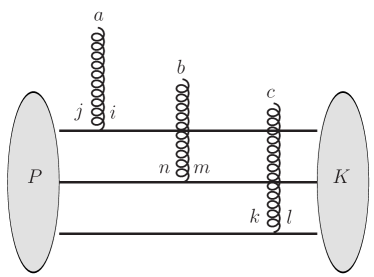
Figure 2: Illustration of the three-body contribution to the $\langle\rho^{a}\rho^{b}\rho^{c}\rangle$ correlator.

III.5.1 One-body contribution

As previously for $\langle{\tilde{\rho}}{\tilde{\rho}}\rangle$, we start with the one-body contribution where all three charge operators act on the same quark. Defining this term as

$$[{\tilde{\rho}}^{a}(q_{1})\,{\tilde{\rho}}^{b}(q_{2})\,{\tilde{\rho}}^{c}(q_{3})]_{1}={\tilde{\rho}}^{a}(q_{1}){\tilde{\rho}}^{b}(q_{2}){\tilde{\rho}}^{c}(q_{3})\otimes 1\!\!1\otimes 1\!\!1+\text{permutations}~{},$$ (54)

we find

$$\langle\,[{\tilde{\rho}}^{a}(q_{1})\,{\tilde{\rho}}^{b}(q_{2})\,{\tilde{\rho}}^{c}(q_{3})]_{1}\,\rangle_{K_{\perp}}=\,\mathrm{tr\,}t^{a}t^{b}t^{c}\int{\rm d}x_{1}{\rm d}x_{2}{\rm d}x_{3}\,\delta(1-x_{1}-x_{2}-x_{3})$$

$$\times \int{{\rm d}^{2}p_{1}{\rm d}^{2}p_{2}{\rm d}^{2}p_{3}\over(16\pi^{3})^{2}}\,\delta(\vec{p}_{1}+\vec{p}_{2}+\vec{p}_{3})\sum_{\lambda_{i}}\psi_{3}^{*}(k_{1},k_{2},k_{3})\,\psi_{3}(p_{1},p_{2},p_{3})~{}.$$

The arguments of $\psi_{3}^{*}$ are $k_{i}^{+}=x_{i}P^{+}$, $\vec{k}_{1}=\vec{p}_{1}+(1-x_{1})\vec{K}_{\perp}$, $\vec{k}_{2}=\vec{p}_{2}-x_{2}\vec{K}_{\perp}$, $\vec{k}_{3}=\vec{p}_{3}-x_{3}\vec{K}_{\perp}$, and all flavors and helicities unchanged ($\lambda_{i}^{\prime}=\lambda_{i}$). The color factor is given by

$$\mathrm{tr\,}\,t^{a}t^{b}t^{c}=\frac{1}{4}d^{abc}+\frac{i}{4}f^{abc}.$$ (56)

Since the $\vec{k}_{i}$ do not explicitly involve the $\vec{q}_{i}$, it follows that at fixed $\vec{K}_{\perp}$, the expectation value of the one-body term is a constant times the delta function constraint on their momentum arguments.

III.5.2 Two-body contribution

The computation of the two-body contribution follows analogously to previously. In this case, two of the charge operators act on one quark, while the third $\rho$-operator acts on a second quark. There are three separate terms, corresponding to the three different possible spectator quarks. The first term can be written as

$$\left[{\tilde{\rho}}^{a}(q_{1})\,{\tilde{\rho}}^{b}(q_{2})\right]_{1}\,\left[{\tilde{\rho}}^{c}(q_{3})\right]_{2} = {\tilde{\rho}}^{a}(q_{1})\,{\tilde{\rho}}^{b}(q_{2})\otimes{\tilde{\rho}}^{c}(q_{3})\otimes 1\!\!1+\text{permutations}~{}.$$ (57)

We then find,

$$\langle\,[{\tilde{\rho}}^{a}(q_{1})\,{\tilde{\rho}}^{b}(q_{2})]_{1}\,[{\tilde{\rho}}^{c}(q_{3})]_{2}\,\rangle_{K_{\perp}}=-\mathrm{tr\,}\,t^{a}t^{b}t^{c}\,\int{\rm d}x_{1}{\rm d}x_{2}{\rm d}x_{3}\,\delta(1-x_{1}-x_{2}-x_{3})$$ (58)

$$\times \int{{\rm d}^{2}p_{1}{\rm d}^{2}p_{2}{\rm d}^{2}p_{3}\over(16\pi^{3})^{2}}\,\delta(\vec{p}_{1}+\vec{p}_{2}+\vec{p}_{3})\sum_{\lambda_{i}}\psi_{3}^{*}(k_{1},k_{2},k_{3})\,\psi_{3}(p_{1},p_{2},p_{3})~{}.$$

Here $k_{i}^{+}=x_{i}P^{+}$, $\vec{k}_{1}=\vec{p}_{1}+\vec{q}_{3}+(1-x_{1})\vec{K}_{\perp}$, $\vec{k}_{2}=\vec{p}_{2}-\vec{q}_{3}-x_{2}\vec{K}_{\perp}$, $\vec{k}_{3}=\vec{p}_{3}-x_{3}\vec{K}_{\perp}$. As usual, all flavors and helicities are kept unchanged ($\lambda_{i}^{\prime}=\lambda_{i}$). For the other two two-body contributions, one needs to exchange $\vec{q}_{3}$ in $\vec{k}_{1}$ and $\vec{k}_{2}$ by $\vec{q}_{1}$ and $\vec{q}_{2}$, respectively. Moreover, the color factor for the expectation value of $[{\tilde{\rho}}^{a}(q_{1})\,{\tilde{\rho}}^{c}(q_{3})]_{1}\,[{\tilde{\rho}}^{b}(q_{2})]_{2}$ is $\mathrm{tr\,}t^{a}t^{c}t^{b}$ instead of $\mathrm{tr\,}t^{a}t^{b}t^{c}$.

Unlike the one-body contributions, these contributions do depend on $\vec{q}_{i}$, even at fixed $t=-K^{2}_{\perp}$. Note that if one writes $\vec{q}=\vec{q}_{1}+\vec{q}_{2}=-\vec{q}_{3}-\vec{K}_{\perp}$ and $\vec{k}=\vec{q}_{3}$, the phase space integral in Eq. (58) is identical to the one which appeared in the two-body contribution to $\left<{\tilde{\rho}}^{a}(q){\tilde{\rho}}^{b}(k)\right>$ in Eq. (LABEL:eq:rho2_Kt). This identity can be seen by direct comparison and serves as a check on the computation.

III.5.3 Three-body contribution

The three-body operator corresponds to each color charge operator acting on separate valence quarks–see Fig. 2. Defining this term as

$$[{\tilde{\rho}}^{a}(q_{1}){\tilde{\rho}}^{b}(q_{2}){\tilde{\rho}}^{c}(q_{3})]_{3}={\tilde{\rho}}^{a}(q_{1})\otimes{\tilde{\rho}}^{b}(q_{2})\otimes{\tilde{\rho}}^{c}(q_{3})+\text{permutations}~{},$$ (59)

we find

$$\langle\,[{\tilde{\rho}}^{a}(q_{1})\,{\tilde{\rho}}^{b}(q_{2})\,{\tilde{\rho}}^{c}(q_{3})]_{3}\,\rangle_{K_{\perp}}=\frac{1}{2}d^{abc}\,\int{\rm d}x_{1}{\rm d}x_{2}{\rm d}x_{3}\,\delta(1-x_{1}-x_{2}-x_{3})$$ (60)

$$\times \int{{\rm d}^{2}p_{1}{\rm d}^{2}p_{2}{\rm d}^{2}p_{3}\over(16\pi^{3})^{2}}\,\delta(\vec{p}_{1}+\vec{p}_{2}+\vec{p}_{3})\sum_{\lambda_{i}}\psi_{3}^{*}(k_{1},k_{2},k_{3})\,\psi_{3}(p_{1},p_{2},p_{3})~{}.$$

Here, $k_{i}^{+}=x_{i}P^{+}$, $\vec{k}_{1}=\vec{p}_{1}-\vec{q}_{1}-x_{1}\vec{K}_{\perp}$, $\vec{k}_{2}=\vec{p}_{2}-\vec{q}_{2}-x_{2}\vec{K}_{\perp}$, $\vec{k}_{3}=\vec{p}_{3}-\vec{q}_{3}-x_{3}\vec{K}_{\perp}$. As usual, all flavors and helicities are unchanged ($\lambda_{i}^{\prime}=\lambda_{i}$). As in the two-body case, this three-body contribution depends on $\vec{q}_{i}$, even at fixed $t=-K^{2}_{\perp}$.

Our net result for $\langle{\tilde{\rho}}^{a}(q_{1}){\tilde{\rho}}^{b}(q_{2}){\tilde{\rho}}^{c}(q_{3})\rangle$ is the sum of Eq. (LABEL:eq:rho3_1body_Kt), Eq. (58) (plus the permutations of momenta indicated below that equation), and Eq. (60). Both the symmetric and antisymmetric structure factors, respectively $d^{abc}$ and $f^{abc}$, are proportional to color charge form factors. Specifically, we can express the symmetric (S) piece as

$$\langle[{\tilde{\rho}}^{a}(q_{1}){\tilde{\rho}}^{b}(q_{2}){\tilde{\rho}}^{c}(q_{3})]_{\rm S}\rangle_{K_{\perp}} \equiv \frac{d^{abc}}{N_{c}}\,\,{\cal G}_{O}(\vec{q}_{1},\vec{q}_{2},\vec{q}_{3};\vec{K}_{\perp})\,,$$ (61)

which involves the 1, 2 and 3-body terms. Anticipating results to appear, we denote ${\cal G}_{O}$ to be the Odderon form factor.

We note that similar form factors were discussed previously in the context of high energy forward scattering amplitudes FukugitaKwiecinski ; Czyzewski:1996bv . Fukugita and Kwiecinski FukugitaKwiecinski similarly identified one-body, two-body and three-body contributions and noted that the two-body contribution can be expressed in terms of the Pomeron form factor in Eq. (39). However, though they suggest that the three-body contribution in Eq. (60) can be expressed in terms of the two body contribution, our results show that this is not true in general. Furthermore, unlike these works, we are able to express our results explicitly in terms of the QCD valence Fock state wavefunction.

We can however confirm the observation in Czyzewski:1996bv that in the limit that any of the $\vec{q}_{i}\to 0$, the sum of all these contributions should vanish. Specifically, taking $\vec{q}_{3}\to 0$ (but $\vec{q}_{1}$, $\vec{q}_{2}$, $\vec{K}_{\perp}$ arbitrary!), one observes that the sum of the $a$, $b$, $c$-symmetric pieces of Eq. (LABEL:eq:rho3_1body_Kt), Eq. (58) and Eq. (60) does indeed vanish. The underlying reason is a general feature of QCD that must be satisfied by any model: a long wavelength gluon cannot couple to a color singlet.

IV Color charge form factors and exclusive heavy quark production in DIS

In the previous section, we derived explicit expressions for the expectation values of quadratic and cubic combinants of the color charge density and reexpressed the results in terms of nonperturbative color charge form factors. We show here that these nonperturbative quantities can be determined from exclusive measurements of heavy Quarkonia in DIS at large $x$ at Jefferson Laboratory Hafidi:2017bsg ; Joosten:2018gyo ; Joosten:2018fql and in the future at an Electron-Ion Collider Accardi:2012qut . We derive the amplitude for exclusive quarkonium production and express it in terms our Pomeron and Odderon color charge form factors in the first subsection. Specifically, we show that the exclusive $J/\Psi$ cross-section is proportional to both the Pomeron and Odderon form factors. In contrast, the $\eta_{c}$ amplitude depends only on the Odderon form factor; the latter can therefore be extracted directly from an exclusive measurement of the production of $\eta_{c}$ mesons. While this possibility is well known in the literature, and even discussed very recently Goncalves:2015hra , we will articulate how our work brings a novel perspective to this discussion.

IV.1 Amplitude for exclusive quarkonium production at large $x_{\rm Bj}$

In DIS at high energies, the amplitude for exclusive quarkonium production be expressed as Kowalski:2006hc

$${\cal A}^{\gamma^{*}\,p\to Q{\bar{Q}}\,p}(Q^{2},\vec{K}_{\perp})\sim i\int{\rm d}^{2}r\int_{0}^{1}\frac{dz}{4\pi}\,\left(\Psi_{\gamma^{*}}\Psi^{*}_{Q{\bar{Q}}}\right)(\vec{r},z,Q^{2})~{}e^{-i\frac{(1-2z)}{2}\vec{r}\cdot\vec{K}_{\perp}}\int d^{2}b_{\perp}\,e^{i{\vec{b}}_{\perp}\cdot\vec{K}_{\perp}}~{}{\cal T}(\vec{r},\vec{b}_{\perp};\vec{K}_{\perp})\,.$$ (62)

Here $\Psi_{\gamma^{*}}$ is the light cone wave function of a virtual photon to fluctuate into a charm-anticharm pair Nikolaev:1990ja of relative size $\vec{r}$, $z$ ($1-z$) is the fraction of the photon momentum taken by the quark (antiquark) and $\vec{K}_{\perp}$ is the transverse momentum transfer between the incoming and outgoing proton. Further, $\Psi_{Q{\bar{Q}}}(\vec{r},z,Q^{2})$ is the wavefunction corresponding to the overlap $\langle c{\bar{c}}|Q{\bar{Q}}\rangle$ of the $c{\bar{c}}$ pair with any $Q{\bar{Q}}$ quarkonium state ($J/\Psi$, $\Psi(2S)$, $\eta_{c}$, $\chi_{c},\cdots$).

Finally, ${\cal T}$ denotes the invariant amplitude for elastic scattering of the $c{\bar{c}}$ pair off color fields in the target proton and can be expressed as Dominguez:2011wm ; Hatta:2017cte ; Roy:2018jxq :

$${\cal T}(\vec{r},\vec{b}_{\perp};\vec{K}_{\perp})=2\,N_{c}\,\left[1-\frac{1}{N_{c}}\,{\rm tr}\,\langle U\left(\vec{b}_{\perp}+\frac{\vec{r}}{2}\right)U^{\dagger}\left(\vec{b}_{\perp}-\frac{\vec{r}}{2}\right)\rangle_{\vec{K}_{\perp}}\right]\,.$$ (63)

Here $U$ (and $U^{\dagger}$) are lightlike Wilson lines representing the color rotation of a color dipole in the gauge field background of the proton. The brackets $\langle\cdots\rangle_{K_{\perp}}$ represent taking the expectation value in the proton according to Eq. (27). As in the discussion there, and discussed further in Appendix A, we are making an eikonal approximation that the proton target has a large $P^{+}$ momentum. In writing Eq. (63), we identified the coordinates $\vec{x}_{T}$ and $\vec{y}_{T}$ of the quark-antiquark pair shown in Fig. 3 with the impact parameter of the quark-antiquark pair and their relative separation respectively as Bartels:2003yj ,

$${\vec{\tilde{b}}_{\perp}} = z{\vec{x}}_{\perp}+(1-z){\vec{y}}_{\perp}\,,$$

$${\vec{r}} = {\vec{x}}_{\perp}-{\vec{y}}_{\perp}\,,$$ (64)

and then a further transformation Hatta:2017cte

$${\vec{b}}_{\perp}={\vec{\tilde{b}}_{\perp}}+\left(\frac{1}{2}-z\right)\,\vec{r}\,,\$$ (65)

to express the result in the symmetric form shown in Eq. (63). The phase factor $e^{-i\frac{(1-2z)}{2}\vec{r}\cdot\vec{K}_{\perp}}$ in Eq. (62) is a consequence of these transformations.

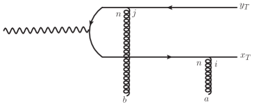
Figure 3: Illustration of the two-gluon contribution to the DIS exclusive amplitude for $c{\bar{c}}$ production.

In Lorenz gauge $\partial_{\mu}A^{\mu}=0$, and in the above described eikonal approximation, the gauge fields appearing in the Wilson lines corresponding to multiple scattering of a quark at spatial position $(x^{-},\vec{x}_{T})$ have only one component $A^{+}$, which satisfies the Poisson equation $\nabla_{\perp}^{2}A^{+}=g\rho(x^{-},\vec{x}_{\perp})\,$ ($A_{\mu}\equiv t^{a}A^{a}_{\mu}$) and the lightlike Wilson lines are path ordered in the $x^{-}$ direction Iancu:2003xm ; Kovchegov:2012mbw :

$$U^{\dagger}(\vec{x}_{T}) = {\cal P}e^{ig\int dx^{-}A^{+}(x^{-},\vec{x}_{T})}$$

$$= 1+ig\int dx^{-}A^{+}(x^{-},\vec{x}_{T})+(ig)^{2}\int dx^{-}\int^{x^{-}}dy^{-}A^{+}(x^{-},\vec{x}_{T})A^{+}(y^{-},\vec{x}_{T})$$

$$+ (ig)^{3}\int dx^{-}\int^{x^{-}}dy^{-}\int^{y^{-}}dz^{-}A^{+}(x^{-},\vec{x}_{T})A^{+}(y^{-},\vec{x}_{T})A^{+}(z^{-},\vec{x}_{T})+\cdots~{}.$$ (67)

where the factors of $g\,t^{a}$ contained in this expansion correspond to the vertices arising from the order by order expansion of the coherent coupling of the gluon fields in the target to the $c$ or $\bar{c}$ quark.

Expanding $U(\vec{x}_{T})U^{\dagger}(\vec{y}_{T})-1$ to third order in $gA^{+}$ gives:

$$1-U(\vec{x}_{T})U^{\dagger}(\vec{y}_{T}) = (ig)^{2}\int dx^{-}\int dy^{-}A^{+}(x^{-},\vec{x}_{T})A^{+}(y^{-},\vec{y}_{T})$$ (68)

$$-(-ig)^{2}\int dx^{-}\int_{x^{-}}dy^{-}A^{+}(x^{-},\vec{x}_{T})A^{+}(y^{-},\vec{x}_{T})$$

$$-(ig)^{2}\int dx^{-}\int^{x^{-}}dy^{-}A^{+}(x^{-},\vec{y}_{T})A^{+}(y^{-},\vec{y}_{T})$$

$$-(-ig)(ig)^{2}\int dx^{-}\int dy^{-}\int^{y^{-}}dz^{-}A^{+}(x^{-},\vec{x}_{T})A^{+}(y^{-},\vec{y}_{T})A^{+}(z^{-},\vec{y}_{T})$$

$$-(-ig)^{2}(ig)\int dx^{-}\int_{x^{-}}dy^{-}\int dz^{-}A^{+}(x^{-},\vec{x}_{T})A^{+}(y^{-},\vec{x}_{T})A^{+}(z^{-},\vec{y}_{T})$$

$$-(-ig)^{3}\int dx^{-}\int_{x^{-}}dy^{-}\int_{y^{-}}dz^{-}A^{+}(x^{-},\vec{x}_{T})A^{+}(y^{-},\vec{x}_{T})A^{+}(z^{-},\vec{x}_{T})$$

$$-(ig)^{3}\int dx^{-}\int^{x^{-}}dy^{-}\int^{y^{-}}dz^{-}A^{+}(x^{-},\vec{y}_{T})A^{+}(y^{-},\vec{y}_{T})A^{+}(z^{-},\vec{y}_{T})+\cdots~{}.$$

Let us first consider the expectation value of the previous expression up to order $(gA^{+})^{2}$. Using the fact that it is symmetric under $x^{-}-y^{-}\to y^{-}-x^{-}$, we can express the term appearing in Eq. (63) as

$$1-\langle U\left(\vec{b}_{\perp}+\frac{\vec{r}}{2}\right)U^{\dagger}\left(\vec{b}_{\perp}-\frac{\vec{r}}{2}\right)\rangle_{K_{\perp}} = -g^{2}\int dx^{-}\int dy^{-}\langle A^{+}\left(x^{-},\vec{b}_{\perp}+\frac{\vec{r}}{2}\right)A^{+}\left(y^{-},\vec{b}_{\perp}-\frac{\vec{r}}{2}\right)\rangle_{K_{\perp}}$$ (69)

$$+ \frac{1}{2}g^{2}\int dx^{-}\int dy^{-}\langle A^{+}\left(x^{-},\vec{b}_{\perp}+\frac{\vec{r}}{2}\right)A^{+}\left(y^{-},\vec{b}_{\perp}+\frac{\vec{r}}{2}\right)\rangle_{K_{\perp}}$$

$$+ \frac{1}{2}g^{2}\int dx^{-}\int dy^{-}\langle A^{+}\left(x^{-},\vec{b}_{\perp}-\frac{\vec{r}}{2}\right)A^{+}\left(y^{-},\vec{b}_{\perp}-\frac{\vec{r}}{2}\right)\rangle_{K_{\perp}}~{}.$$

We can use the Poisson equation to relate $A^{+}$ to the charge density operator $\rho$ and further, to write the latter in terms of its two-dimensional Fourier representation. In doing so, note that the integral of ${\tilde{\rho}}(x^{-},\vec{q})$ over $x^{-}$ corresponds to the operator ${\tilde{\rho}}(q)$ in Eq. (25). We then obtain, to quadratic order in $A^{+}$ or $\rho$,

$$1-\frac{1}{N_{c}}{\rm tr}\langle U\left(\vec{b}_{\perp}+\frac{\vec{r}}{2})\right)U^{\dagger}\left(\vec{b}_{\perp}-\frac{\vec{r}}{2}\right)\rangle_{\vec{K}_{\perp}}^{O(\rho^{2})} = -\frac{g^{4}}{2N_{c}}\,\delta^{ab}\int\limits_{q_{1}}\int\limits_{q_{2}}\frac{e^{i{\vec{b}}_{\perp}\cdot({\vec{q}_{1}}+{\vec{q}_{2}})}}{q_{1}^{2}q_{2}^{2}}\left[e^{i\frac{\vec{r}}{2}\cdot({\vec{q_{1}}}-{\vec{q_{2}}})}-\frac{1}{2}e^{i(q_{1}+q_{2})\cdot\frac{\vec{r}}{2}}-\frac{1}{2}e^{-i(q_{1}+q_{2})\cdot\frac{\vec{r}}{2}}\right]$$ (70)

$$\times \langle{\tilde{\rho}}^{a}(\vec{q}_{1}){\tilde{\rho}}^{b}(\vec{q}_{2})\rangle_{\vec{K}_{\perp}}~{}.$$

Multiplying both l.h.s and r.h.s by $2N_{c}$ to obtain ${\cal T}^{O(\rho^{2})}$, we can then perform the integration over impact parameter in Eq. (62) to obtain

$$\int d^{2}b_{\perp}e^{i{\vec{b}}_{\perp}\cdot\vec{K}_{\perp}}~{}{\cal T}^{O(\rho^{2})}(\vec{r},\vec{b}_{\perp};\vec{K}_{\perp}) = 2\,N_{c}\,\left[-\frac{g^{4}}{2N_{c}}\,\int_{q_{1}}\frac{1}{q_{1}^{2}(\vec{q}_{1}+\vec{K}_{\perp})^{2}}\,\left(e^{i\frac{{\vec{r}}}{2}\cdot(2{\vec{q}_{1}}+\vec{K}_{\perp})}-\cos\left(\frac{{\vec{r}}\cdot\vec{K}_{\perp}}{2}\right)\right)\right.$$ (71)

$$\times \langle{\tilde{\rho}}^{a}({\vec{q}_{1}}){\tilde{\rho}}^{a}(-{\vec{q}_{1}}-\vec{K}_{\perp})\rangle_{K_{\perp}}\Bigg{]}~{}.$$

Defining the l.h.s of the above expression to be the Pomeron amplitude ${\cal P}(\vec{r},\vec{K}_{\perp})$ and replacing $\langle{\tilde{\rho}}(\vec{q}_{1}){\tilde{\rho}}(-{\vec{q}_{1}}-\vec{K}_{\perp})\rangle_{\vec{K}_{T}}$ on the r.h.s by the Pomeron form factor in Eq. (38), we obtain,

$${\cal P}(\vec{r},\vec{K}_{\perp})=2\,N_{c}\left[-\frac{g^{4}C_{F}}{2}\,\int_{q_{1}}\frac{1}{q_{1}^{2}\,(\vec{q}_{1}+\vec{K}_{\perp})^{2}}\,\left(e^{i\frac{{\vec{r}}}{2}\cdot(2{\vec{q}_{1}}+\vec{K}_{\perp})}-\cos\left(\frac{{\vec{r}}\cdot\vec{K}_{\perp}}{2}\right)\right){\cal G}({\vec{q}_{1}},-{\vec{q}_{1}}-\vec{K}_{\perp})\right]~{}.$$ (73)

Here $C_{F}=(N_{c}^{2}-1)/2N_{c}$ is the quadratic Casimir in the fundamental representation.

The amplitude for exclusive quarkonium production in DIS can also receive a contribution from three-gluon exchange, as illustrated in Fig. 4.

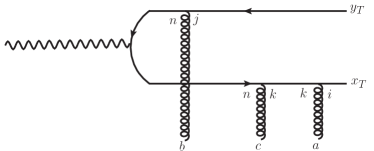
Figure 4: Illustration of the three-gluon contribution to the DIS exclusive amplitude for $c{\bar{c}}$ production.

This contribution is recovered in our approach by expanding Eq. (63) to $O(\rho^{3})$. We begin by formally rewriting

$${\cal T}(\vec{r},\vec{b}_{\perp};\vec{K}_{\perp}) = 2\,N_{c}\Bigg{[}1-\frac{1}{2N_{c}}{\rm tr}\left(\langle U\left(\vec{b}_{\perp}+\frac{\vec{r}}{2}\right)U^{\dagger}\left(\vec{b}_{\perp}-\frac{\vec{r}}{2}\right)\rangle_{\vec{K}_{\perp}}+\langle U\left(\vec{b}_{\perp}-\frac{\vec{r}}{2}\right)U^{\dagger}\left(\vec{b}_{\perp}+\frac{\vec{r}}{2}\right)\rangle_{\vec{K}_{\perp}}\right)$$ (74)

$$- \frac{1}{2N_{c}}{\rm tr}\left(\langle U\left(\vec{b}_{\perp}+\frac{\vec{r}}{2}\right)U^{\dagger}\left(\vec{b}_{\perp}-\frac{\vec{r}}{2}\right)\rangle_{\vec{K}_{\perp}}-\langle U\left(\vec{b}_{\perp}-\frac{\vec{r}}{2}\right)U^{\dagger}\left(\vec{b}_{\perp}+\frac{\vec{r}}{2}\right)\rangle_{\vec{K}_{\perp}}\right)\Bigg{]}\,.$$

as the sum of a piece that’s symmetric under $\vec{b}_{\perp}+\frac{\vec{r}}{2}\leftrightarrow\vec{b}_{\perp}-\frac{\vec{r}}{2}$ and a piece that is antisymmetric under this exchange. Expanding out both the symmetric and antisymmetric terms to $O((gA^{+})^{3})$, or equivalently $O(\rho^{3})$, we find that the symmetric piece is identically zero at this order. In other words, its impossible to have color-singlet three-gluon exchange that is even under parity. The contribution of the surviving term can be expressed as the Odderon amplitude

$$i{\cal O}(\vec{r},\vec{K}_{\perp}) = \int d^{2}b_{\perp}e^{i{\vec{b}}_{\perp}\cdot\vec{K}_{\perp}}~{}{\cal T}^{O(\rho^{3})}(\vec{r},\vec{b}_{\perp};\vec{K}_{\perp})\,,$$ (75)

where

$${\cal T}^{O(\rho^{3})}(\vec{r},\vec{b}_{\perp};\vec{K}_{\perp})=\frac{1}{2N_{c}}{\rm tr}\left(\langle U\left(\vec{b}_{\perp}+\frac{\vec{r}}{2}\right)U^{\dagger}\left(\vec{b}_{\perp}-\frac{\vec{r}}{2}\right)\rangle_{K_{\perp}}-\langle U\left(\vec{b}_{\perp}-\frac{\vec{r}}{2}\right)U^{\dagger}\left(\vec{b}_{\perp}+\frac{\vec{r}}{2}\right)\rangle_{\vec{K}_{\perp}}\right)$$ (76)

has the form of the expectation value of the Odderon operator Hatta:2005as .

Working the r.h.s out to cubic order in $gA^{+}$ (or equivalently $\rho$)–see Appendix B for details–one obtains

$${\cal T}^{O(\rho^{3})}({\vec{r}},{\vec{b}_{\perp}};\vec{K}_{\perp}) = -\frac{g^{6}}{8N_{c}}d^{abc}\int\limits_{q_{1}}\int\limits_{q_{2}}\int\limits_{q_{3}}\frac{1}{q_{1}^{2}}\frac{1}{q_{2}^{2}}\frac{1}{q_{3}^{2}}\,\langle{\tilde{\rho}}^{a}(\vec{q}_{1}){\tilde{\rho}}^{b}(\vec{q}_{2}){\tilde{\rho}}^{c}(\vec{q}_{3})\rangle_{K_{\perp}}\,e^{i{\vec{b}_{\perp}}\cdot({\vec{q}_{1}}+{\vec{q}_{2}}+{\vec{q}_{3}})}$$ (77)

$$\times \left[2\sin\left(\frac{{\vec{r}}}{2}\cdot({\vec{q}_{1}}-{\vec{q}_{2}}-{\vec{q}_{3}})\right)+\frac{2}{3}\sin\left(\frac{{\vec{r}}}{2}\cdot({\vec{q}_{1}}+{\vec{q}_{2}}+{\vec{q}_{3}})\right)\right]~{}.$$

Note that only the terms proportional to $\sim d^{abc}$ from $\langle\rho^{a}(\vec{q}_{1})\rho^{b}(\vec{q}_{2})\rho^{c}(\vec{q}_{3})\rangle_{K_{\perp}}$ contribute. Further, employing our definition of the Odderon amplitude in Eq. (61), and using the identity

$$d^{abc}d^{abe}=\frac{N_{c}^{2}-4}{N_{c}}\,\delta^{ce}\,,$$ (78)

we obtain the Odderon amplitude to be

$$i{\cal O}(\vec{r};\vec{K}_{\perp}) = -g^{6}\frac{(N_{c}^{2}-4)(N_{c}^{2}-1)}{8N_{c}^{3}}\int\limits_{q_{1}}\int\limits_{q_{2}}\frac{1}{q_{1}^{2}}\frac{1}{q_{2}^{2}}\frac{1}{(\vec{q}_{1}+\vec{q}_{2}+\vec{K}_{\perp})^{2}}\,{\cal G}_{O}(\vec{q}_{1},\vec{q}_{2},-\vec{K}_{\perp}-\vec{q}_{1}-\vec{q}_{2};\vec{K}_{\perp})$$ (79)

$$\times \left[2\sin\left(\frac{{\vec{r}}}{2}\cdot(2{\vec{q}_{1}}+\vec{K}_{\perp})\right)-\frac{2}{3}\sin\left(\frac{{\vec{r}}}{2}\cdot\vec{K}_{\perp}\right)\right]~{}\,,$$

where ${\cal G}_{O}(\vec{q}_{1},\vec{q}_{2},-\vec{K}_{\perp}-\vec{q}_{1}-\vec{q}_{2};\vec{K}_{\perp})$ is the Odderon form factor from Eq. (61) and $(N_{c}^{2}-1)(N_{c}^{2}-4)/4\,N_{c}^{2}=C_{3F}$ is the cubic Casimir constant of SU($N_{c}$) in the fundamental representation.

The Odderon expectation value $iO(\vec{x}_{T},\vec{y}_{T};K_{T}=0)$ in the forward limit has been computed previously in the MV model, where the weight functional (appropriately normalized) describing the distribution of color charges in a large nucleus has the general form Jeon:2004rk ; Jeon:2005cf ,

$$W[\rho]=\int[d\rho]\,\exp\left(-\int d^{2}x_{\perp}\left[\frac{\rho^{a}(\vec{x}_{\perp})\rho^{a}(\vec{x}_{\perp})}{2\mu^{2}}-\frac{d_{abc}\,\rho^{a}(\vec{x}_{\perp})\rho^{b}(\vec{x}_{\perp})\rho^{c}(\vec{x}_{\perp})}{\kappa_{A}}\right]\right)\,.$$ (80)

The cubic Casimir term here has the weight $\kappa_{A}=g^{3}A^{2}N_{c}/\pi^{2}R^{4}$ and will of course give a non-zero value for the Odderon form factor. For a large nucleus, if the typical magnitude of $\rho\sim\sqrt{\mu_{\rm MV}^{2}}\sim A^{1/6}$, this cubic Odderon term is subleading relative to the quadratic Pomeron term in $W[\rho]$ by $A^{-1/6}$, which is a weak suppression factor even for a large nucleus. The expectation value $iO(x_{T},y_{T})$ of the Odderon operator computed in the MV model gives

$$iO(\vec{x}_{T},\vec{y}_{T})=\alpha_{S}^{3}\frac{(N_{c}^{2}-4)(N_{c}^{2}-1)}{4\pi r_{0}^{2}N_{c}^{3}}\,A^{1/3}\,\int d^{2}{\bf u}\,\ln^{3}\frac{|{\bf x}-{\bf u}|}{|{\bf y}-{\bf u}|}\,,$$ (81)

where $r_{0}=1.12$ fm. This expression is also recovered in a perturbative QCD computation Kovchegov:2003dm . We can compare this expression to Eq. (79), for $A\rightarrow 1$ and in the forward limit of $\vec{K}_{T}\rightarrow 0$. As discussed in Jeon:2005cf , the logarithm above can be expressed in terms of the Coulomb propagator in two dimensions. Making use of this fact, we observe that Eq. (81) can be reexpressed as Eq. (79) if the Odderon form factor ${\cal G}_{O}$ is a constant everywhere except in the infrared due to the previously discussed constraint from color neutrality. Conversely, the structure of ${\cal G}_{O}$ in Eq. (79), and hence the Odderon operator at large $x_{\rm Bj}$, can be very different from the expectation from the MV model.

IV.2 Cross-section for exclusive production of $J/\Psi$ and $\eta_{c}$ mesons at large $x_{\rm Bj}$

The general formalism for exclusive quarkonium production that we outlined in the previous section can now be adapted to compute the cross-section for specific quarkonium states. We will consider here the $J/\Psi$ because it is the most easily accessible Onium state, and the $\eta_{c}$ because it is the lightest state with unique features that promise novel insight into nonperturbative QCD. Since we are interested in many-body color charge correlators of valence Fock states in this work, our discussion is most relevant for exclusive production of these quarkonium states at large $x_{\rm Bj}$. As noted, this is a regime that is already accessible with the high luminosity DIS experiments at Jefferson Lab and at a future EIC.

The cross-section for exclusive $J/\Psi$ production can be expressed as

$$\frac{d\sigma_{T,L}^{\gamma^{*}p\rightarrow J/\Psi\,p}}{dt}=\frac{1}{16\pi}|\,{\cal A}_{T,L}^{\gamma^{*}p\rightarrow J/\Psi p}\,|^{2}\,,$$ (82)

where

$${\cal A}_{T,L}^{\gamma^{*}p\rightarrow J/\Psi p}(Q^{2},\vec{K}_{\perp})\sim i\int{\rm d}^{2}r\int\frac{dz}{4\pi}\,\left(\Psi_{\gamma^{*}}\Psi^{*}_{J/\Psi}\right)(\vec{r},z,Q^{2})~{}e^{-i\frac{(1-2z)}{2}\vec{r}\cdot\vec{K}_{\perp}}\,\left[{\cal P}(\vec{r},\vec{K}_{\perp})+i{\cal O}(\vec{r},\vec{K}_{\perp})\right]\,.$$ (83)

Here $K_{\perp}^{2}=-t$, and $\Psi_{J/\Psi}$, $\Psi_{\gamma^{*}}$ denote the $J/\psi$ and virtual photon light cone wave functions (for longitudinal or transverse polarization); their product is summed over the helicities of the $c$ and $\bar{c}$ quarks. Further, ${\cal P}$ is the Pomeron contribution to the exclusive $J/\Psi$ amplitude given in Eq. (73) and $i{\cal O}$ is the respective Odderon contribution given by Eq. (79). The former is directly proportional to the Pomeron color charge form factor and the latter to the Odderon color charge form factor. These two terms in ${\cal A}_{T,L}^{\gamma^{*}p\rightarrow J/\Psi\,p}$ contain the important QCD physics underlying the Regge theory based descriptions of elastic/exclusive cross-sections in terms of imaginary and real terms respectively Forshaw:1997dc . There is an additional kinematic contribution coming from the non-zero values of $\Delta x$ discussed in Section II; however, as we demonstrate in Appendix A, these contributions are $1/P^{+}$ suppressed.

Some remarks on the contribution due to the Odderon are in order. $i{\cal O}$ is odd under charge conjugation, which corresponds to the simultaneous transformations $\vec{r}\to-\vec{r}$, $z\to 1-z$. On the other hand, $\Psi_{\gamma^{*}}\Psi^{*}_{J/\Psi}$ has even C parity. Therefore, the integral over $i{\cal O}$ in Eq. (83) is non-zero only if the final state is restricted to, for example, $p^{+}_{c}<p^{+}_{\bar{c}}$ ($z<1/2$). This prevents the cancellation of the amplitude with its C conjugate. Likewise, the Odderon contribution to the above amplitude will not cancel against its parity transform if the direction of the momentum transfer $\vec{K}_{\perp}$ is fixed. The role of such charge asymmetry and kinematic constraints in Pomeron-Odderon DIS amplitudes has been noted previously for other final states Brodsky:1999mz ; Hagler:2002nf .

The two-gluon Pomeron and three-gluon Odderon form factors were discussed previously in Brodsky:2000zc albeit this work did not identify these form factors as such. More importantly, we have provided explicit first-principles expressions for the Pomeron form factor in Eq. (39) and likewise for the Odderon form factor in Eq. (61) in terms of the QCD light front wavefunction for valence Fock states. Therefore exclusive measurements of the $J/\Psi$ at large $x_{\rm Bj}$ offer the opportunity to extract fundamental nonperturbative QCD physics contained in these wavefunctions.

It is important to note that by large $x_{\rm Bj}$, we have $x_{\rm Bj}\approx 0.1$ in mind. At larger values of $x_{\rm Bj}$, our approximations ignoring $\Delta x$ are no longer tenable. At smaller values of $x_{\rm Bj}<0.1$, higher gluon Fock states become important. While these can be incorporated in our approach, and matched eventually to the CGC EFT framework, their treatment is outside the scope of the present discussion.

We observed that that while the exclusive $J/\Psi$ cross-section is dominated by the Pomeron contribution, it can in principle be sensitive to the Odderon form factor for particular kinematics. In contrast to the $J/\psi$ however, the $\eta_{c}$ meson with its $P=-1$ and $C=+1$ quantum numbers, is dominantly produced in exclusive DIS by the three-gluon color singlet Odderon exchange contribution. The exclusive $\eta_{c}$ production amplitude is simply

$${\cal A}_{T,L}^{\gamma^{*}p\rightarrow\eta_{c}p}(Q^{2},\vec{K}_{\perp})\sim i\int{\rm d}^{2}r\int\frac{dz}{4\pi}\,\left(\Psi_{\gamma^{*}}\,\Psi^{*}_{\eta_{c}}\right)(\vec{r},z,Q^{2})~{}e^{-i\frac{(1-2z)}{2}\vec{r}\cdot\vec{K}_{\perp}}\,i{\cal O}(\vec{r},\vec{K}_{\perp})\,,$$ (84)

where $\Psi_{\eta_{c}}$ is the light cone $\eta_{c}$ wavefunction. Indeed, exclusive $\eta_{c}$ was proposed some time ago Schaefer as the cleanest channel for discovery of the Odderon where the focus there was on $\eta_{c}$ production at small $x_{\rm Bj}$ at HERA. Ref. Engel:1997cga followed the approach of FukugitaKwiecinski ; Czyzewski:1996bv to estimate the HERA DIS $\eta_{c}$ cross-section to be 47 pb for photo-production and 11 pb for $Q^{2}=5$ GeV². However FukugitaKwiecinski ; Czyzewski:1996bv express the Odderon form factor in terms of that of the Pomeron form factor. Our study shows that this assumption is likely unjustified; we plan to investigate its quantitative impact in a future publication.

Searches at HERA did not reveal any evidence for exclusive $\eta_{c}$. From the theory perspective, this may be because the Odderon amplitude is suppressed at small $x$. While not definitive, studies of the small $x$ evolution of the Odderon suggest that its energy dependence is much smaller than that of the Pomeron Bartels:1999yt ; it may even decrease with increasing energy Janik:1998xj ; Lappi:2016gqe . Therefore, searches at larger values of $x_{\rm Bj}$ may be more promising. Further, since the cross-section for such exclusive processes is small, such searches will benefit from the much higher luminosities at Jefferson Lab and in future at the EIC.

V Summary and Outlook

In this paper, we developed a novel formalism within the framework of light front QCD to compute color charge correlators and their associated color charge form factors. For simplicity, we constructed the quadratic $\langle\rho\rho\rangle$ and cubic $\langle\rho\rho\rho\rangle$ correlators of valence quark Fock states in the proton. The extension of our computation to include gluon and sea quark color charge densities is straightforward if more involved. These quadratic and cubic color charge correlators are precisely the color singlet two-gluon Pomeron form factor and the three-gluon Odderon form factor respectively. They capture important nonperturbative physics on the spatio-temporal distribution of color charges in the proton, and offer a complementary description of this tomography to that offered by TMDs and GPDs. Further, they provide useful classical intuition at the level of the Yang-Mills dynamics of QCD. As a striking example, note that the Wong equations Wong:1970fu satisfied by classical color charges in background gauge fields are embedded in the structure of the QCD effective action JalilianMarian:1999xt . Classical intuition at this level can motivate experimental searches for novel QCD effects.

While expressing observables in terms of expectation values of color charge correlators is uncommon at large $x$ (see however Burkardt:2003yg ), it is a key feature of the Color Glass Condensate framework at small $x$, whereby dynamical many-body information from nonperturbative initial conditions is encoded in a gauge invariant density matrix $W[\rho]$. For a large nucleus, this quantity is the Gaussian weight functional of the McLerran-Venugopalan model. However, this formalism breaks down for the proton at large $x$ and the initial conditions for small $x$ evolution of color charge correlations in the proton have a significant source of uncertainty arising from the initial conditions.

We showed that exclusive measurements of quarkonia at large $x$ allow for independent extraction of $\langle\rho\rho\rangle$ and $\langle\rho\rho\rho\rangle$. Expectation values of these, and the associated Pomeron and Odderon color charge form factors, can be extracted from clean exclusive DIS measurements of quarkonium final states at large $x$. These form factors, and in principle higher moments of the color charge density, therefore provide a bridge between small $x$ and large $x$ in QCD, one that is constrained by high energy proton-proton and proton-nucleus experiments on multiparticle correlations at RHIC and and LHC on the one hand, and DIS experiments at Jefferson Lab on the other. We also applied the formalism towards computing the gluon distribution of a proton, and obtained sensible results. We anticipate that the Electron-Ion Collider, which will have an unparalleled combination of $x$ reach and high luminosities, will bring powerful new insight into the underlying dynamics of many-body color charge correlations in QCD.

Another interesting avenue of research that presents itself is the extraction of color charge correlations and form factors in polarized deep inelastic scattering and polarized proton-proton collisions. Odderon exchange can for instance be probed in the single spin asymmetries measured in polarized proton-proton collisions Kovchegov:2012ga . Single spin asymmetries in semi-inclusive open charge production in polarized DIS are also sensitive to the Odderon operator Zhou:2013gsa ; Dong:2018wsp . These connections between color charge form factors in a wide range of experiments are ripe for further exploration.

Appendix A: $P^{+}$ limit of the density operator, and the parton pancake

Consider Eq. (23). This contains a term:

$$P^{+}e^{i(x_{q}-x_{p})P^{+}r^{-}},$$ (85)

which oscillates like crazy if $P^{+}\to\infty$ unless $r^{-}$ or/and $(x_{p}-x_{q})$ vanishes. In those cases the term is infinite. This is suggestive of delta functions, and the pancake shape of high energy projectiles.

To better understand the term Eq. (85) consider a test function $f(r^{-})$ which is continuous at the origin and non-zero over a finite region of space. Such would arise in taking the matrix element of the density operator in the proton wave function. Then

$$\int dr^{-}f(r^{-})\lim_{P^{+}\to\infty}P^{+}e^{i(x_{q}-x_{p})P^{+}r^{-}}$$

$$=\lim_{P^{+}\to\infty}\int due^{i(x_{q}-x_{p})u}f(u/P^{+})$$

$$=f(0)\int due^{i(x_{q}-x_{p})u}=f(0)2\pi\delta(x_{q}-x_{p}).$$ (86)

Thus the term of Eq. (85) and the density operator of Eq. (23) acts as a delta function in both $x_{q}-x_{p}$ and $r^{-}$.

Thus effectively

$$\lim_{P^{+}\to\infty}P^{+}e^{i(x_{q}-x_{p})P^{+}r^{-}}\rightarrow 2\pi\delta(x_{p}-x_{q})\delta(r^{-}).$$ (87)

We therefore see that the density $\rho^{a}(r)$ contains $\delta(r^{-})$, hence the pancake shape. Using Eq. (87) in Eq. (23) and integrating over $r^{-}$ leads immediately to Eq. (26).

The corrections of order $1/P^{+}$ can be understood from Eq. (86), by using

$$f(u/P^{+})\approx f(0)+f^{\prime}(0){u\over P^{+}}.$$ (88)

Including the second term gives a correction term:

$${2\pi i\over P^{+}}f^{\prime}(0){\partial\over\partial x_{q}}\delta(x_{q}-x_{p}).$$ (89)

Appendix B: The Odderon amplitude in terms of the Odderon form factor

The Odderon contribution to the amplitude in Eq. (75) can be written our explicitly as

$$\frac{1}{2N_{c}}\,\text{tr}~{}\langle U(\vec{x}_{T})U^{\dagger}(\vec{y}_{T})-U(\vec{y}_{T})U^{\dagger}(\vec{x}_{T})\rangle_{K_{\perp}}=$$ (91)

$$\frac{ig^{3}}{2N_{c}}\,\text{tr}\left<\int dx^{-}\int dy^{-}\int^{y^{-}}dz^{-}A^{+}(x^{-},\vec{x}_{T})A^{+}(y^{-},\vec{y}_{T})A^{+}(z^{-},\vec{y}_{T})\right.$$

$$- \int dx^{-}\int dy^{-}\int^{y^{-}}dz^{-}A^{+}(x^{-},\vec{y}_{T})A^{+}(y^{-},\vec{x}_{T})A^{+}(z^{-},\vec{x}_{T})$$ (92)

$$- \int dx^{-}\int_{x^{-}}dy^{-}\int dz^{-}A^{+}(x^{-},\vec{x}_{T})A^{+}(y^{-},\vec{x}_{T})A^{+}(z^{-},\vec{y}_{T})$$ (93)

$$+ \int dx^{-}\int_{x^{-}}dy^{-}\int dz^{-}A^{+}(x^{-},\vec{y}_{T})A^{+}(y^{-},\vec{y}_{T})A^{+}(z^{-},\vec{x}_{T})$$ (94)

$$+ \int dx^{-}\int_{x^{-}}dy^{-}\int_{y^{-}}dz^{-}A^{+}(x^{-},\vec{x}_{T})A^{+}(y^{-},\vec{x}_{T})A^{+}(z^{-},\vec{x}_{T})$$ (95)

$$- \int dx^{-}\int_{x^{-}}dy^{-}\int_{y^{-}}dz^{-}A^{+}(x^{-},\vec{y}_{T})A^{+}(y^{-},\vec{y}_{T})A^{+}(z^{-},\vec{y}_{T})$$ (96)

$$- \int dx^{-}\int^{x^{-}}dy^{-}\int^{y^{-}}dz^{-}A^{+}(x^{-},\vec{y}_{T})A^{+}(y^{-},\vec{y}_{T})A^{+}(z^{-},\vec{y}_{T})$$ (97)

$$+ \left.\int dx^{-}\int^{x^{-}}dy^{-}\int^{y^{-}}dz^{-}A^{+}(x^{-},\vec{x}_{T})A^{+}(y^{-},\vec{x}_{T})A^{+}(z^{-},\vec{x}_{T})\right>_{K_{\perp}}~{}.$$ (98)

With a little algebra one can combine Eq. (91) and Eq. (94) to

$$\text{tr}~{}t^{a}t^{b}t^{c} \int dx^{-}\int dy^{-}\int dz^{-}A^{+a}(z^{-},x_{T})A^{+b}(x^{-},y_{T})A^{+c}(y^{-},y_{T})$$ (99)

$$= \frac{1}{4}d^{abc}\int dx^{-}\int dy^{-}\int dz^{-}A^{+a}(z^{-},x_{T})A^{+b}(x^{-},y_{T})A^{+c}(y^{-},y_{T})~{}.$$

In the last step we have used that the factor multiplying $\text{tr}~{}t^{a}t^{b}t^{c}$ is symmetric under $b\leftrightarrow c$. Since all fields are now integrated over $x^{-}$ without limits they can be traded for $\rho^{a}(q)$ from eq. (25) so that the previous line becomes

$$\frac{g^{3}}{4}d^{abc}\int\limits_{q_{1}}\int\limits_{q_{2}}\int\limits_{q_{3}}\frac{1}{q_{1}^{2}}\frac{1}{q_{2}^{2}}\frac{1}{q_{3}^{2}}\,e^{i(q_{1}\cdot x_{T}+(q_{2}+q_{3})\cdot y_{T})}\,\rho^{a}(q_{1})\rho^{b}(q_{2})\rho^{c}(q_{3})~{}.$$ (100)

Along the same lines, the sum of (92) and (93) can be rewritten as

$$-\frac{1}{4}d^{abc}\int dx^{-}\int dy^{-}\int dz^{-}A^{+a}(z^{-},y_{T})A^{+b}(x^{-},x_{T})A^{+c}(y^{-},x_{T})$$ (101)

$$= -\frac{g^{3}}{4}d^{abc}\int\limits_{q_{1}}\int\limits_{q_{2}}\int\limits_{q_{3}}\frac{1}{q_{1}^{2}}\frac{1}{q_{2}^{2}}\frac{1}{q_{3}^{2}}\,e^{i(q_{1}\cdot y_{T}+(q_{2}+q_{3})\cdot x_{T})}\,\rho^{a}(q_{1})\rho^{b}(q_{2})\rho^{c}(q_{3})~{}.$$

The remaining terms from eqs. (95-98) involve integrals over $A^{+}(x^{-},x_{T})$ at the same point $x_{T}$, i.e. integrals of the same (matrix valued) function $A^{+}(x^{-})$. One may thus use standard identities for “time” ordered exponentials of a matrix $A(t)$:

$$T~{}\int dt_{1}\cdots\int dt_{n}A(t_{1})\cdots A(t_{n})=T~{}\int dt_{1}\cdots\int dt_{n}\frac{1}{n!}\,\sum_{\text{p}erm}A(t_{i_{1}})\cdots A(t_{i_{n}})~{}.$$ (102)

The sum is over all permutations of $A(t_{1})$, $A(t_{2}),\cdots,A(t_{n})$. We can now express (95)+(98) as

$$2\frac{1}{3!}\frac{1}{4}d^{abc}\int dx^{-}\int dy^{-}\int dz^{-}A^{+a}(x^{-},\vec{x}_{T})A^{+b}(y^{-},\vec{x}_{T})A^{+c}(z^{-},\vec{x}_{T})$$ (103)

$$= \frac{g^{3}}{12}d^{abc}\int\limits_{q_{1}}\int\limits_{q_{2}}\int\limits_{q_{3}}\frac{1}{q_{1}^{2}}\frac{1}{q_{2}^{2}}\frac{1}{q_{3}^{2}}\,e^{i(q_{1}+q_{2}+q_{3})\cdot x_{T}}\,\rho^{a}(q_{1})\rho^{b}(q_{2})\rho^{c}(q_{3})~{}.$$

Similarly, the sum of (96) and (97) is given by

$$-\frac{1}{12}d^{abc}\int dx^{-}\int dy^{-}\int dz^{-}A^{+a}(x^{-},\vec{y}_{T})A^{+b}(y^{-},\vec{y}_{T})A^{+c}(z^{-},\vec{y}_{T})$$ (104)

$$= -\frac{g^{3}}{12}d^{abc}\int\limits_{q_{1}}\int\limits_{q_{2}}\int\limits_{q_{3}}\frac{1}{q_{1}^{2}}\frac{1}{q_{2}^{2}}\frac{1}{q_{3}^{2}}\,e^{i(q_{1}+q_{2}+q_{3})\cdot y_{T}}\,\rho^{a}(q_{1})\rho^{b}(q_{2})\rho^{c}(q_{3})~{}.$$

References

- (1) D. Boer et al., arXiv:1108.1713 [nucl-th].
- (2) J. Dudek et al., Eur. Phys. J. A 48, 187 (2012)
- (3) X. d. Ji, Phys. Rev. Lett. 91, 062001 (2003)
- (4) E. P. Wigner, Phys. Rev. 40, 749 (1932).
- (5) D. Mueller, D. Robaschik, B. Geyer, F.-M. Dittes and J. Horejsi, Fortsch. Phys. 42, 101 (1994)
- (6) X. D. Ji, Phys. Rev. Lett. 78, 610 (1997)
- (7) A. V. Radyushkin, Phys. Lett. B 380, 417 (1996)
- (8) J. C. Collins, L. Frankfurt and M. Strikman, Phys. Rev. D 56, 2982 (1997).
- (9) M. Burkardt, Int. J. Mod. Phys. A 18, 173 (2003).
- (10) M. Diehl, Phys. Rept. 388, 41 (2003).
- (11) A. V. Belitsky and A. V. Radyushkin, Phys. Rept. 418, 1 (2005).
- (12) J. P. Ralston and D. E. Soper, Nucl. Phys. B 152, 109 (1979).
- (13) J. C. Collins and D. E. Soper, Nucl. Phys. B 193, 381 (1981) Erratum: [Nucl. Phys. B 213, 545 (1983)].
- (14) P. J. Mulders and R. D. Tangerman, Nucl. Phys. B 461, 197 (1996) Erratum: [Nucl. Phys. B 484, 538 (1997)].
- (15) D. Boer and P. J. Mulders, Phys. Rev. D 57, 5780 (1998).
- (16) A. V. Belitsky, X. Ji and F. Yuan, Nucl. Phys. B 656, 165 (2003).
- (17) G. A. Miller, Phys. Rev. C 68, 022201 (2003); G. A. Miller, Nucl. Phys. News 18, 12 (2008); G. A. Miller, Phys. Rev. C 76, 065209 (2007).
- (18) V. Punjabi, C. F. Perdrisat, M. K. Jones, E. J. Brash and C. E. Carlson, Eur. Phys. J. A 51, 79 (2015).
- (19) G. A. Miller, Phys. Rev. Lett. 99, 112001 (2007).
- (20) G. A. Miller, Ann. Rev. Nucl. Part. Sci. 60, 1 (2010).
- (21) C. E. Carlson and M. Vanderhaeghen, Phys. Rev. Lett. 100, 032004 (2008).
- (22) M. Burkardt, Phys. Rev. D 62, 071503 (2000); Erratum: [Phys. Rev. D 66, 119903 (2002)].
- (23) F. Dominguez, C. Marquet, B. W. Xiao and F. Yuan, Phys. Rev. D 83, 105005 (2011).
- (24) E. Petreska, Int. J. Mod. Phys. E 27, no. 05, 1830003 (2018).
- (25) O. Hen, G. A. Miller, E. Piasetzky and L. B. Weinstein, Rev. Mod. Phys. 89, no. 4, 045002 (2017).
- (26) G. A. Miller, M. D. Sievert and R. Venugopalan, Phys. Rev. C 93, no. 4, 045202 (2016).
- (27) F. Winter, W. Detmold, A. S. Gambhir, K. Orginos, M. J. Savage, P. E. Shanahan and M. L. Wagman, Phys. Rev. D 96, no. 9, 094512 (2017).
- (28) E. Iancu and R. Venugopalan, In *Hwa, R.C. (ed.) et al.: Quark gluon plasma* 249-3363 [hep-ph/0303204].
- (29) F. Gelis, E. Iancu, J. Jalilian-Marian and R. Venugopalan, Ann. Rev. Nucl. Part. Sci. 60, 463 (2010).
- (30) Y. V. Kovchegov and E. Levin, Cambridge Monogr. Math. Phys. 33 (2012).
- (31) J. P. Blaizot, Rept. Prog. Phys. 80, no. 3, 032301 (2017).
- (32) L. D. McLerran and R. Venugopalan, Phys. Rev. D 49, 2233 (1994).
- (33) L. D. McLerran and R. Venugopalan, Phys. Rev. D 49, 3352 (1994).
- (34) L. D. McLerran and R. Venugopalan, Phys. Rev. D 50, 2225 (1994).
- (35) Y. V. Kovchegov, Phys. Rev. D 54, 5463 (1996).
- (36) S. Jeon and R. Venugopalan, Phys. Rev. D 70, 105012 (2004).
- (37) L. V. Gribov, E. M. Levin and M. G. Ryskin, Phys. Rept. 100, 1 (1983).
- (38) A. H. Mueller and J. w. Qiu, Nucl. Phys. B 268, 427 (1986).
- (39) A. Ayala, J. Jalilian-Marian, L. D. McLerran and R. Venugopalan, Phys. Rev. D 52, 2935 (1995).
- (40) J. Jalilian-Marian, A. Kovner, L. D. McLerran and H. Weigert, Phys. Rev. D 55, 5414 (1997).
- (41) A. H. Mueller, Nucl. Phys. B 335, 115 (1990).
- (42) A. H. Mueller, Nucl. Phys. B 558, 285 (1999).
- (43) L. D. McLerran and R. Venugopalan, Phys. Rev. D 59, 094002 (1999).
- (44) Y. V. Kovchegov, Phys. Rev. D 60, 034008 (1999).
- (45) R. Venugopalan, Acta Phys. Polon. B 30, 3731 (1999).
- (46) J. Jalilian-Marian, A. Kovner, A. Leonidov and H. Weigert, Phys. Rev. D 59, 014014 (1998).
- (47) J. Jalilian-Marian, A. Kovner and H. Weigert, Phys. Rev. D 59, 014015 (1998).
- (48) E. Iancu, A. Leonidov and L. D. McLerran, Nucl. Phys. A 692, 583 (2001) [hep-ph/0011241].
- (49) E. Ferreiro, E. Iancu, A. Leonidov and L. McLerran, Nucl. Phys. A 703, 489 (2002) [hep-ph/0109115].
- (50) I. Balitsky, Nucl. Phys. B 463, 99 (1996).
- (51) H. Weigert, Nucl. Phys. A 703, 823 (2002).
- (52) J. P. Blaizot, E. Iancu and H. Weigert, Nucl. Phys. A 713, 441 (2003).
- (53) K. Rummukainen and H. Weigert, Nucl. Phys. A 739, 183 (2004).
- (54) E. A. Kuraev, L. N. Lipatov and V. S. Fadin, Sov. Phys. JETP 45, 199 (1977).
- (55) I. I. Balitsky and L. N. Lipatov, Sov. J. Nucl. Phys. 28, 822 (1978).
- (56) E. Iancu, K. Itakura and L. McLerran, Nucl. Phys. A 724, 181 (2003).
- (57) A. H. Mueller, Phys. Lett. B 523, 243 (2001).
- (58) A. Dumitru, J. Jalilian-Marian, T. Lappi, B. Schenke and R. Venugopalan, Phys. Lett. B 706, 219 (2011).
- (59) T. Lappi and H. Mantysaari, Phys. Rev. D 88, 114020 (2013).
- (60) J. Kuokkanen, K. Rummukainen and H. Weigert, Nucl. Phys. A 875, 29 (2012).
- (61) J. L. Albacete, N. Armesto, J. G. Milhano, P. Quiroga-Arias and C. A. Salgado, Eur. Phys. J. C 71, 1705 (2011).
- (62) F. Gelis and R. Venugopalan, Nucl. Phys. A 776, 135 (2006).
- (63) F. Gelis and R. Venugopalan, Nucl. Phys. A 779, 177 (2006).
- (64) F. Gelis, T. Lappi and R. Venugopalan, Int. J. Mod. Phys. E 16, 2595 (2007).
- (65) F. Gelis, T. Lappi and R. Venugopalan, Phys. Rev. D 78, 054019 (2008).
- (66) F. Gelis, T. Lappi and R. Venugopalan, Phys. Rev. D 78, 054020 (2008).
- (67) Y. V. Kovchegov and A. H. Mueller, Nucl. Phys. B 529, 451 (1998).
- (68) A. Dumitru and L. D. McLerran, Nucl. Phys. A 700, 492 (2002).
- (69) K. Dusling, W. Li and B. Schenke, Int. J. Mod. Phys. E 25, no. 01, 1630002 (2016).
- (70) B. Schenke and R. Venugopalan, Phys. Rev. Lett. 113, 102301 (2014).
- (71) J. D. Bjorken, S. J. Brodsky and A. Scharff Goldhaber, Phys. Lett. B 726, 344 (2013).
- (72) K. Dusling, M. Mace and R. Venugopalan, PoS QCDEV 2017, 039 (2018), arXiv:1801.09704 [hep-ph].
- (73) L. McLerran and V. Skokov, Nucl. Phys. A 959, 83 (2017)
- (74) D. Boer, T. Van Daal, P. J. Mulders and E. Petreska, arXiv:1805.05219 [hep-ph].
- (75) Y. V. Kovchegov and V. V. Skokov, Phys. Rev. D 97, no. 9, 094021 (2018).
- (76) M. Mace, V. V. Skokov, P. Tribedy and R. Venugopalan, arXiv:1805.09342 [hep-ph].
- (77) H. Mäntysaari and B. Schenke, Phys. Rev. Lett. 117, no. 5, 052301 (2016).
- (78) J. L. Albacete and A. Soto-Ontoso, Phys. Lett. B 770, 149 (2017).
- (79) P. Bozek, W. Broniowski and M. Rybczynski, Phys. Rev. C 94, no. 1, 014902 (2016).
- (80) S. J. Brodsky, H. C. Pauli and S. S. Pinsky, Phys. Rept. 301, 299 (1998).
- (81) L. Lukaszuk and B. Nicolescu, Lett. Nuovo Cim. 8, 405 (1973).
- (82) G. Antchev et al. [TOTEM Collaboration], Submitted to: Phys.Rev., CERN-EP-2017-335.
- (83) S. J. Brodsky and G. P. Lepage, Adv. Ser. Direct. High Energy Phys. 5, 93 (1989).
- (84) S. J. Brodsky, D. S. Hwang, B. Q. Ma and I. Schmidt, Nucl. Phys. B 593, 311 (2001).
- (85) A. Krasnitz, Y. Nara and R. Venugopalan, Nucl. Phys. A 717, 268 (2003).
- (86) R. V. Gavai and R. Venugopalan, Phys. Rev. D 54, 5795 (1996).
- (87) C. S. Lam and G. Mahlon, Phys. Rev. D 61, 014005 (2000).
- (88) E. Iancu and L. D. McLerran, Phys. Lett. B 510, 145 (2001).
- (89) J. F. Gunion and D. E. Soper, Phys. Rev. D 15, 2617 (1977).
- (90) F. Schlumpf, Phys. Rev. D 47, 4114 (1993) Erratum: [Phys. Rev. D 49, 6246 (1994)].
- (91) M. R. Frank, B. K. Jennings and G. A. Miller, Phys. Rev. C 54, 920 (1996).
- (92) G. A. Miller, Phys. Rev. C 66, 032201 (2002).
- (93) B. Pasquini and S. Boffi, Phys. Rev. D 76, 074011 (2007).
- (94) B. Pasquini, S. Boffi and P. Schweitzer, Mod. Phys. Lett. A 24, 2903 (2009).
- (95) C. Lorce, B. Pasquini and M. Vanderhaeghen, JHEP 1105, 041 (2011).
- (96) I. C. Cloet and G. A. Miller, Phys. Rev. C 86, 015208 (2012).
- (97) Y. V. Kovchegov, L. Szymanowski and S. Wallon, Phys. Lett. B 586, 267 (2004).
- (98) M. Fukugita and J. Kwiecinski, Phys. Lett. 83B, 119 (1979).
- (99) J. Czyzewski, J. Kwiecinski, L. Motyka and M. Sadzikowski, Phys. Lett. B 398, 400 (1997) Erratum: [Phys. Lett. B 411, 402 (1997)], [hep-ph/9611225].
- (100) K. Hafidi, S. Joosten, Z. E. Meziani and J. W. Qiu, Few Body Syst. 58, no. 4, 141 (2017).
- (101) S. Joosten and Z. E. Meziani, PoS QCDEV 2017, 017 (2018).
- (102) S. Joosten, arXiv:1803.08615 [hep-ph].
- (103) A. Accardi et al., Eur. Phys. J. A 52, no. 9, 268 (2016).
- (104) V. P. Goncalves and W. K. Sauter, Phys. Rev. D 91, no. 9, 094014 (2015).
- (105) H. Kowalski, L. Motyka and G. Watt, Phys. Rev. D 74, 074016 (2006) [hep-ph/0606272].
- (106) N. N. Nikolaev and B. G. Zakharov, Z. Phys. C 49, 607 (1991).
- (107) Y. Hatta, B. W. Xiao and F. Yuan, Phys. Rev. D 95, no. 11, 114026 (2017).
- (108) K. Roy and R. Venugopalan, JHEP 1805, 013 (2018) [arXiv:1802.09550 [hep-ph]].
- (109) J. Bartels, K. J. Golec-Biernat and K. Peters, Acta Phys. Polon. B 34, 3051 (2003) [hep-ph/0301192].
- (110) Y. Hatta, E. Iancu, K. Itakura and L. McLerran, Nucl. Phys. A 760, 172 (2005).
- (111) S. Jeon and R. Venugopalan, Phys. Rev. D 71, 125003 (2005).
- (112) A. Dumitru, J. Jalilian-Marian and E. Petreska, Phys. Rev. D 84, 014018 (2011) [arXiv:1105.4155 [hep-ph]]; A. Dumitru and E. Petreska, Nucl. Phys. A 879, 59 (2012) [arXiv:1112.4760 [hep-ph]].
- (113) J. R. Forshaw and D. A. Ross, Cambridge Lect. Notes Phys. 9, 1 (1997).
- (114) S. J. Brodsky, J. Rathsman and C. Merino, Phys. Lett. B 461, 114 (1999) doi:10.1016/S0370-2693(99)00807-2 [hep-ph/9904280].
- (115) P. Hägler, B. Pire, L. Szymanowski and O. V. Teryaev, Eur. Phys. J. C 26, 261 (2002) doi:10.1140/epjc/s2002-01054-9 [hep-ph/0207224].
- (116) S. J. Brodsky, E. Chudakov, P. Hoyer and J. M. Laget, Phys. Lett. B 498, 23 (2001).
- (117) C. Ewerz, hep-ph/0306137.
- (118) A. Schäfer, L. Mankiewicz and O. Nachtmann, in Proc. of the Workshop Physics at HERA, Hamburg (October 29-31, 1991), Ed. W. Buchmüller and G. Ingelman.
- (119) R. Engel, D. Y. Ivanov, R. Kirschner and L. Szymanowski, Eur. Phys. J. C 4, 93 (1998), [hep-ph/9707362].
- (120) J. Bartels, L. N. Lipatov and G. P. Vacca, Phys. Lett. B 477, 178 (2000).
- (121) R. A. Janik and J. Wosiek, Phys. Rev. Lett. 82, 1092 (1999).
- (122) T. Lappi, A. Ramnath, K. Rummukainen and H. Weigert, Phys. Rev. D 94, no. 5, 054014 (2016) [arXiv:1606.00551 [hep-ph]].
- (123) A. H. Mueller, hep-ph/9911289.
- (124) S. K. Wong, Nuovo Cim. A 65, 689 (1970).
- (125) J. Jalilian-Marian, S. Jeon, R. Venugopalan and J. Wirstam, Phys. Rev. D 62, 045020 (2000).
- (126) M. Burkardt, Phys. Rev. D 69, 057501 (2004).
- (127) Y. V. Kovchegov and M. D. Sievert, Phys. Rev. D 86, 034028 (2012) Erratum: [Phys. Rev. D 86, 079906 (2012)].
- (128) J. Zhou, Phys. Rev. D 89, no. 7, 074050 (2014).
- (129) H. Dong, D. X. Zheng and J. Zhou, arXiv:1805.09479 [hep-ph].
- (130) D. Binosi and L. Theußl, Comp. Phys. Comm. 161, 76 (2004).