Lensing and imaging by a stealth defect of spacetime

Abstract

We obtain the geodesics for the simplest possible stealth defect which has a flat spacetime. We, then, discuss the lensing properties of such a defect, and the corresponding image formation. Similar lensing properties can be expected to hold for curved-spacetime stealth defects.

Journal: Mod. Phys. Lett. A 34 (2019) 1950026
       Preprint: arXiv:1808.02465
PACS Nos.: 04.20.Cv, 04.20.Gz, 98.62.Sb

1 Introduction

A particular Skyrmion spacetime defect has been studied recently in a series of papers: the self-consistent Anzätze for the fields were established in Ref. 1, the origin of a possible negative asymptotic gravitational mass was discussed in Ref. 2, and the details of a special defect solution with zero asymptotic gravitational mass were given in Ref. 3. This last defect solution, with positive energy density of the matter fields but a vanishing asymptotic gravitational mass, has been called a “stealth defect.”

It was stated in Sec. 4 of Ref. 3 that “assuming the existence of this particular type of spacetime-defect solution without long-range fields, an observer has no advance warning if he/she approaches such a stealth-type defect solution (displacement effects of background stars are negligible, at least initially).” The goal of the present article is to expand on the parenthetical remark of the previous quote. We study, in particular, the geodesics of the special defect solution of Fig. 5 in Ref. 3, which has a flat spacetime. For completeness, we have also performed a simplified calculation of the geodesics for a curved-spacetime stealth defect and present the results in A.

It may be helpful to place the present paper in context before we start our somewhat technical discussion. The important point to realize is that the spacetime manifolds discussed in Refs. 1, 2, 3 are genuine solutions of the standard Einstein equation, but with a nontrivial spacetime topology and a degenerate metric (regarding this last characteristic, see, in particular, the second and third remarks in Sec. VI of Ref. 2). The analysis of the main part of the present paper is for an exact solution of the vacuum Einstein equation, namely the flat-spacetime defect solution. The analysis in the Appendix of the present paper is for an approximation of the numerical solution of the Einstein and matter-field equations. The results in the Appendix are, therefore, only indicative.

Another point that needs to be clarified in advance is the order of magnitude of the defect length scale $b$, as defined in Sec. 2 and the caption of Fig. 1. In Sec. 6, we will briefly discuss a “gas” of identical static defects. In that case, the experimental data are consistent with having a highly-rarified gas of microscopic static defects (e.g., $b\sim l_{\text{planck}}\equiv\sqrt{8\pi G_{N}\,\hbar/c^{3}}\approx 8.10\times 10^{-35}\;\text{m}$ and a typical distance between the individual defects of order $l\gg b$). Still, nothing excludes having, in a remote part of the Universe, a single spacetime defect with a macroscopic value of its length scale (e.g., $b\sim\text{Mpc}\approx 3.09\times 10^{22}\;\text{m}$).

2 Geodesic equations

The topology and coordinatization of the spacetime manifold considered has been reviewed in Sec. 2 of Ref. 4 and Sec. II D of Ref. 5 (see also Chap. 3 of Ref. 6 for the proper definition of the field equations). Very briefly, the spatial part of the manifold is obtained by removing the interior of a ball in three-dimensional Euclidean space and by identifying antipodal points on the boundary of this ball (the defect surface has topology $\mathbb{R}P^{2}\sim S^{2}/\mathbb{Z}_{2}$). As to the coordinatization, there are three coordinate charts. Here, we focus on the chart-2 coordinates, the other charts being similar. Moreover, we use dimensionless coordinates, all lengths being measured in units of $1/(e\,f)>0$ for the theory as defined in Ref. 3.

The metric of a particular defect-type solution of the vacuum Einstein equation reads as follows (cf. Sec. 3 of Ref. 4):

$$ds^{2}\,\Big{|}^{\text{(vac.\,sol.)}} = -\left(1-l/\sqrt{w}\,\right)\,(dt)^{2}+\frac{1-y_{0}^{2}/w}{1-l/\sqrt{w}}\;(dy)^{2}$$ (2.1a)

$$+w\,\Big{[}(dz)^{2}+\sin^{2}z\,(dx)^{2}\Big{]}\,,$$

$$w \equiv y_{0}^{2}+y^{2}\,,$$ (2.1b)

$$y_{0} \equiv e\,f\,b>0\,,$$ (2.1c)

where $y_{0}$ corresponds to the dimensionless version of the defect length scale $b>0$. Note that we only show the dimensionless chart-2 coordinates. Specifically, the spatial chart-2 coordinates have the following ranges:

$$x \in (0,\pi)\,,$$ (2.2a)

$$y \in (-\infty,\infty)\,,$$ (2.2b)

$$z \in (0,\pi)\,,$$ (2.2c)

where $x$ and $z$ are angular coordinates and $y$ is a dimensionless quasi-radial coordinate with $y=0$ corresponding to the defect surface ($y$ is positive one side of the defect and negative on the other).

For a globally regular solution, the real constant $l$ in (2.1a) takes the following values:

$$l\in(-\infty,\,y_{0})\,.$$ (2.3)

With $l=0$ for the stealth-defect solution from Sec. 2.4 and Fig. 5 in Ref. 3, we have the metric

$$ds^{2}\,\Big{|}^{(\text{vac.\,sol.}\;l=0)}=-(dt)^{2}+A(y)\;(dy)^{2}+w\,\Big{[}(dz)^{2}+\sin^{2}z\,(dx)^{2}\Big{]}\,,$$ (2.4a)

with

$$A(y)=\frac{y^{2}}{y_{0}^{2}+y^{2}}\,$$ (2.4b)

and $w$ defined by (2.1b). Then, the nonvanishing Christoffel symbols are

$$\Gamma^{y}_{\hphantom{y}yy} = \frac{A^{\prime}}{2A}\,,$$ (2.5a)

$$\Gamma^{y}_{\hphantom{y}zz} = -\frac{w^{\prime}}{2A}\,,$$ (2.5b)

$$\Gamma^{y}_{\hphantom{y}xx} = -\frac{w^{\prime}\sin^{2}z}{2A}\,,$$ (2.5c)

$$\Gamma^{z}_{\hphantom{z}yz} = \Gamma^{z}_{\hphantom{z}zy}=\frac{w^{\prime}}{2w}\,,$$ (2.5d)

$$\Gamma^{z}_{\hphantom{z}xx} = -\sin z\cos z\,,$$ (2.5e)

$$\Gamma^{x}_{\hphantom{x}yx} = \Gamma^{x}_{\hphantom{x}xy}=\frac{w^{\prime}}{2w}\,,$$ (2.5f)

$$\Gamma^{x}_{\hphantom{x}zx} = \Gamma^{x}_{\hphantom{x}xz}=\cot z\,,$$ (2.5g)

where the prime stands for differentiation with respect to $y$. The first three Christoffel symbols are divergent at the defect surface, but our results will show that the motion of a particle can still be regular.

From the geodesic equation [7] with affine parameter $\lambda$, we find

$$0 = \frac{d^{2}t}{d\lambda^{2}}\,,$$ (2.6a)

$$0 = \frac{d^{2}y}{d\lambda^{2}}+\Gamma^{y}_{\hphantom{y}yy}\left(\frac{dy}{d\lambda}\right)^{2}+\Gamma^{y}_{\hphantom{y}zz}\left(\frac{dz}{d\lambda}\right)^{2}+\Gamma^{y}_{\hphantom{y}xx}\left(\frac{dx}{d\lambda}\right)^{2}\,,$$ (2.6b)

$$0 = \frac{d^{2}z}{d\lambda^{2}}+2\Gamma^{z}_{\hphantom{z}yz}\frac{dy}{d\lambda}\frac{dz}{d\lambda}+\Gamma^{z}_{\hphantom{z}xx}\left(\frac{dx}{d\lambda}\right)^{2}\,,$$ (2.6c)

$$0 = \frac{d^{2}x}{d\lambda^{2}}+2\Gamma^{x}_{\hphantom{x}yx}\frac{dy}{d\lambda}\frac{dx}{d\lambda}+2\Gamma^{x}_{\hphantom{x}zx}\frac{dx}{d\lambda}\frac{dz}{d\lambda}\,.$$ (2.6d)

We can choose the normalization of $\lambda$ so that the solution of (2.6a) has

$$\frac{dt}{d\lambda}=1\,.$$ (2.7)

Then, $\lambda$ can be replaced by $t$ in (2.6b), (2.6c), and (2.6d). Since the metric is spherically symmetric, we need only consider the case $z=\pi/2$. Our calculation follows Sec. 8.4 of Ref. 7.

For the case $dx/dt\neq 0$, divide (2.6d) by $dx/dt$ and use the Christoffel symbols from (2.5). We, then, have

$$\frac{d}{\textbullet dt}\left(\ln\frac{dx}{dt}+\ln w\right)=0\,,$$ (2.8)

which gives a real constant (up to a sign),

$$J\equiv w\,\frac{dx}{dt}\,.$$ (2.9)

With (2.5), (2.9), and multiplying (2.6b) by $2A\,dy/dt$, we find

$$\frac{d}{dt}\left[A\left(\frac{dy}{dt}\right)^{2}+\frac{J^{2}}{w}\right]=0\,.$$ (2.10)

Hence, there is the following constant of motion:

$$E\equiv A\left(\frac{dy}{dt}\right)^{2}+\frac{J^{2}}{w}\,.$$ (2.11)

By elimination of $t$ from (2.9) and (2.11), we get $y$ as a function of $x$,

$$\frac{A}{w^{2}}\left(\frac{dy}{dx}\right)^{2}+\frac{1}{w}=\frac{E}{J^{2}}\,.$$ (2.12)

From (2.9), (2.11), and $z=\pi/2$, the metric (2.4) along the geodesic can now be written as

$$ds^{2}=(-1+E)(dt)^{2}\,.$$ (2.13)

In other words, we have

$$E = 1\,,\qquad\;\;\;\text{for a massless particle}\,,$$ (2.14a)

$$E \in [0,\,1)\,,\quad\text{for a massive particle}\,,$$ (2.14b)

where the case $E=0$ corresponds to $dy/dt=0$, as will be discussed in Sec. 3.

3 Radial geodesics

Consider the geodesic equation for a particle moving exactly in the negative $y$ direction (going from right to left in Fig. 1), i.e., $dx/dt=0$. From the definition of $J$ in (2.9), it follows immediately that $J=0$, even though $J$ was initially defined as a nonzero quantity [see the sentence at the start of the paragraph above (2.8)]. The corresponding energy-type constant of motion is

$$E=\frac{y^{2}}{y_{0}^{2}+y^{2}}\left(\frac{dy}{dt}\right)^{2}\,.$$ (3.1)

The solutions of (3.1) are

$$y = \pm\sqrt{-y_{0}^{2}+\left(+\sqrt{E}\,t+C_{1}\right)^{2}}\,,$$ (3.2a)

$$y = \pm\sqrt{-y_{0}^{2}+\left(-\sqrt{E}\,t+C_{2}\right)^{2}}\,,$$ (3.2b)

where $C_{1}$ and $C_{2}$ are real constants.

Making appropriate time shifts (or setting $C_{1}=C_{2}=y_{0}$) and defining $B\equiv\sqrt{E}/y_{0}$, the solutions (3.2) reproduce the results of Sec. 3 in Ref. 4. Finally, as mentioned below (2.14b), we find a constant $y$ solution if $E=0$.

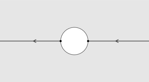
Figure 1: Radial geodesic for the stealth defect (2.4), with part of the 3-dimensional space manifold indicated by the shaded area and antipodal points (dots) on the defect surface identified. The “long distance” between the dots equals $\pi b$, where $b$ is the defect length scale.

4 Nonradial geodesics

Nonradial geodesics exist in two types, those which cross the defect surface ($\mathbb{R}P^{2}\sim S^{2}/\mathbb{Z}_{2}$) and those which do not.

4.1 Geodesics not crossing the defect surface

Outside the defect surface, the spacetime (2.4) is Minkowskian with vanishing curvature invariants [4]. So, geodesics which do not cross the defect surface should be straight lines with standard Cartesian coordinates. The following calculation will show this explicitly.

From (2.12), we find

$$dx=\pm\int\frac{y\,dy}{(y_{0}^{2}+y^{2})\sqrt{(E/J^{2})\,(y_{0}^{2}+y^{2})-1}}\,.$$ (4.1)

Define the quasi-radial coordinate $y_{1}$ corresponding to the point on the line closest to the defect surface (cf. Fig. 2 with $y_{1}>0$), so that $|y_{1}|$ corresponds to an “impact parameter.” Since $d\sqrt{w}/dx$ and $dy/dx$ vanish at $y_{1}$, (2.12) gives

$$\frac{1}{y_{0}^{2}+y_{1}^{2}}=\frac{E}{J^{2}}\,.$$ (4.2)

Then, (4.1) can be written as

$$x(y)=x(\infty)\pm\int^{\infty}_{y}\frac{y\,dy}{(y_{0}^{2}+y^{2})\sqrt{(y_{0}^{2}+y^{2})/(y_{0}^{2}+y_{1}^{2})-1}}\,.$$ (4.3)

At $y=y_{1}$, (4.3) gives

$$|x(y_{1})-x(\infty)|=\pi/2\,.$$ (4.4)

The result (4.4) shows that these particular geodesics (nonradial and nonintersecting with the defect surface) are indeed straight lines.

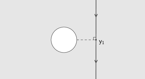
Figure 2: Nonradial geodesic which does not cross the defect surface and defines the quasi-radial coordinate $y_{1}>0$.

4.2 Geodesics crossing the defect surface

Now, consider nonradial geodesics which cross the defect surface. If we use in (2.12) the replacement

$$\frac{dy}{dx}=\frac{1}{2y}\,\frac{dy^{2}}{dx}\,,$$ (4.5)

we find the following two solutions for $y^{2}$:

$$y^{2} = \frac{\tan^{2}(x_{1}+x)+1}{E/J^{2}}-y_{0}^{2}\,,$$ (4.6a)

$$y^{2} = \frac{\tan^{2}(x_{2}-x)+1}{E/J^{2}}-y_{0}^{2}\,,$$ (4.6b)

where $x_{1}$ and $x_{2}$ are real constants.

Note that the metric (2.4) has a spherically symmetric form and that the corresponding “radial” coordinate is $\sqrt{w}\in[y_{0},\infty)$. After a shift of the constants, the solutions (4.6) can be written as

$$\sqrt{w}\,\sin(x_{1}-x) = \pm\frac{J}{\sqrt{E}}\,,$$ (4.7a)

$$\sqrt{w}\,\sin(x_{2}+x) = \pm\frac{J}{\sqrt{E}}\,,$$ (4.7b)

with $\sqrt{w}\geq y_{0}$. Several comments on the solutions (4.7) are in order:

1. mathematically, the solutions are straight lines or straight-line segments in polar-type coordinates ($\sqrt{w},\,x$);

2. the solutions are regular at the defect surface, $\sqrt{w}=y_{0}\,$;

3. to find the complete geodesic of a given particle among these solutions, we must remember the antipodal identifications at the defect surface $\sqrt{w}=y_{0}$.

For a nonradial ingoing line, it is convenient to choose coordinates, so that the end of the ingoing line has $x=\pi/2$ (Fig. 5). In these coordinates, the ingoing line is given by

$$\sqrt{w}\sin(x_{0}-x) = -y_{0}\cos x_{0}\,,$$ (4.8a)

with

$$0<x_{0}<x\leq\pi/2\,.$$ (4.8b)

Observe that we have included the end point of the ingoing line in (4.8b). We can check that the formula (4.8) indeed corresponds to one of the solutions (4.7).

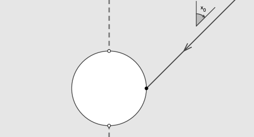
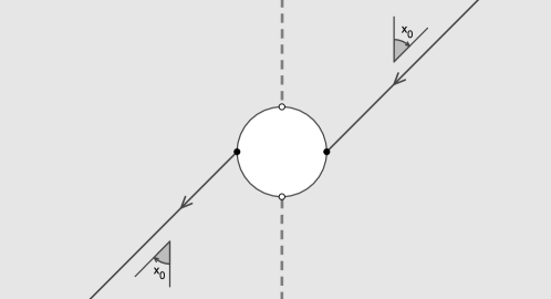
Figure 3: Ingoing line (4.8) lying in the domain of the chart-2 coordinates. The dashed line shows the $x_{3}$ Cartesian axis, which does not belong to the domain of the chart-2 coordinates [5].

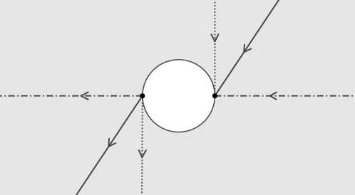
Figure 4: Nonradial geodesic crossing the defect surface.

Figure 5: Family of geodesics crossing the defect surface.

In this case, there will exist, among the solutions (4.7), a unique outgoing line (Fig. 5) if the following two conditions are met:

1. the beginning of the outgoing line and the end of the ingoing line must be antipodal points at the defect surface (these points are identified);

2. the complete geodesic must be a straight line if $y_{0}=0$.

Note that, with a nonradial ingoing line as in Fig. 5, the quantity $J$ will change sign after crossing the defect surface (see Ref. 5 for further discussion of the anomalous angular-momentum behavior of scattering solutions). Based on the above two points, Fig. 5 shows three geodesics from a continuous family of geodesics crossing the defect surface: the family ranges continuously from a radial geodesic (dot-dashed line) to a tangent geodesic (dotted line).

From the particular family of geodesics as shown in Fig. 5, we obtain what may be called a “shifted tangent geodesic” (dotted line in Fig. 5). But, from the limiting case of the geodesic in Fig. 2 with $y_{1}\to 0^{+}$, we obtain what may be called an “ongoing tangent geodesic” (solid line in Fig. 2 pushed towards the defect surface). Hence, we conclude that “certain geodesics at the defect surface $y=0$ cannot be continued uniquely,” as mentioned in the second remark of Sec. VI in Ref. 2 (further discussion can be found in Sec. 3.1.5 of Ref. 6).

5 Image formation by a flat-spacetime stealth defect

The geodesics of the stealth-defect spacetime (2.4) have been discussed in Secs. 3 and 4. For a nonradial geodesic reaching the defect surface, Fig. 5 shows that the defect causes a parallel shift of the geodesic in the ambient space (i.e., the Euclidean 3-space away from the defect surface). In this section, we will show that this shift can, in principle, create an image of a given object.

First, consider geodesics which start from a point $P$ at one side of the defect (Fig. 7). For geodesics which cross the defect surface, there will be an intersection point $P^{\prime}$ at the other side of the defect. In fact, $P$ and $P^{\prime}$ are reflection points about the “center” of the defect (considered to be obtained by surgery on the three-dimensional Euclidean space). The different paths connecting $P$ and $P^{\prime}$ have, in general, different values for the time-of-flight.

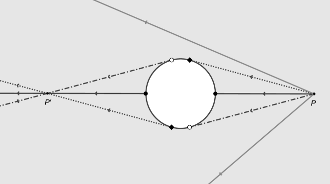
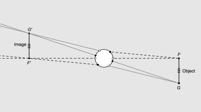
Figure 6: Geodesics with intersection points $P$ and $P^{\prime}$.

Figure 7: Image formation by a stealth defect.

Next, observe that, based on the above discussion for the geodesics of a stealth-defect spacetime, a permanent luminous object will give a real image of the object (Fig. 7). The qualification “permanent” for the light source refers to the different time-of-flight values mentioned in the previous paragraph.

Several additional remarks are in order. First, the image in Fig. 7 is located at the reflection point on the other side of the defect.

Second, the image is inverted and the image size is equal to the object size. Note that this is also the case if an object in Minkowski spacetime is located at a $2f$ distance from a standard thin double-convex lens, where $f$ is the focal length of the lens (cf. Sec. 27.3 of Ref. 8). Recall that the time-of-flight of different paths connecting the $2f$ points of a standard lens in Minkowski spacetime is equal, due to the reduced speed of light in the lens material and the appropriate shape of the lens.

Third, if we consider the image from a static luminous source, then the irradiance of the image depends on both the defect scale $b$ and the location of the source (the irradiance is defined as the power per unit receiving area; cf. Secs. 5.3.2 and 5.3.5 of Ref. 9). The irradiance will be larger if $b$ is increased for an unchanged source position (larger “white disk” in Fig. 7) or if the source is brought closer to the defect for an unchanged defect scale (object and image closer to the “white disk” in Fig. 7): in both cases, the flux captured and transmitted by the defect is larger.

Fourth, return to the analogy with standard lenses in Minkowski spacetime as mentioned in the second remark and note that our defect resembles a so-called zoom lens, with a finite range of focal lengths. If we recall the standard lens equation $1/d_{\text{object}}+1/d_{\text{image}}=1/f$ in Minkowski spacetime [cf. Eq. (27.12) of Ref. 8], we see that our defect has an effective focal length $f_{\text{eff}}$ given by

$$2\,f_{\text{eff }}=\sqrt{b^{2}+(Y_{\text{object}})^{2}}\in(b,\,\infty)\,,$$ (5.1)

where $Y_{\text{object}}\equiv y_{\text{object}}/(ef)\neq 0$ is the dimensional chart-2 quasi-radial coordinate of a small object away from the defect surface.

Fifth, if a permanent pointlike light source is placed at point $P$ of Fig. 7, then an observer at point $P^{\prime}$ in the same figure will see a luminous disk (different from the Einstein ring [10, 11, 12, 13, 14, 15], which the observer would see if the defect were replaced by a patch of Minkowski spacetime with a static spherical star at the center).

Sixth, it may be of interest to compare our lensing and imaging results from the spacetime defect with those from wormholes (see, e.g., Refs. 12, 16, 17, 18 and references therein). In both cases, there is an unusual ingredient in the physics setup: exotic matter for the wormholes and a degenerate metric for the spacetime defect.

6 Discussion

In the present article, we have studied the geodesics of the static $l=0$ stealth-defect solution (2.4), which has a flat spacetime. This exact solution of the vacuum Einstein equation results in Ref. 3 from the parameter choice $\widetilde{\eta}\equiv 8\pi\,G_{N}\,f^{2}=0$ for $G_{N}=0$ and $f>0$.

Incidentally, exact multi-defect solutions of the vacuum Einstein equation are obtained by superposition of these static $l=0$ defects, as long as the individual defect surfaces do not intersect. (Tight experimental bounds for such a Lorentz-violating “gas” of defects have been obtained in Refs. 19, 20.) It may even be possible to obtain an exact multi-defect solution of the vacuum Einstein equation which is approximately Lorentz invariant by superposition of quasi-randomly positioned and quasi-randomly moving $l=0$ defects (arranged to be nonintersecting, at least initially). In addition to the expected broadening of light beams (a Brownian-motion-type effect), such a Lorentz-invariant gas of defects may lead to mass-generation effects [21].

Remark that the $l(w)\neq 0$ stealth-defect solution of Fig. 4 in Ref. 3 has a curved spacetime (parameter choice $\widetilde{\eta}=1/10$), which results in some additional bending of light passing near the defect surface. In fact, the bending is outwards, as the effective mass near the defect surface is negative; see the $l(w)$ panel of Fig. 4 in Ref. 3 and the definition of $l(w)$ in the sentence below (A.1c) in the Appendix of the present article. Still, the lensing property is essentially the same as for the flat-spacetime defect (see A for a simplified calculation).

In the lensing argument of Sec. 5 for the $l=0$ flat-spacetime defect, we considered light rays. But, with the particle–wave duality, we can also interpret the three geodesics crossing the defect surface in Fig. 7 as coherent light emitted from the source $P$ (as mentioned before, the emission is assumed to last for a long time). At the point $P^{\prime}$, these coherent-light bundles have a constant (time-independent) phase difference, which ​leads to stationary interference. In this sense, our defect resembles not only a material lens in Minkowski spacetime but also some type of interferometer (the behavior depends primarily on the ratio of the wavelength $\lambda$ and the defect length scale $b$).

As a final comment, we contrast the lensing from our hypothetical spacetime defect with standard gravitational lensing [10, 11, 12, 13, 14, 15]. Standard gravitational lensing can be interpreted as being due to the curvature of spacetime resulting from a nonvanishing matter distribution. The lensing of Fig. 7 is, however, entirely due to the nontrivial topology from the defect, as the spacetime manifold of this particular solution is flat.

Appendix A Geodesics of a curved-spacetime stealth defect

In Sec. 5, we have shown that a particular defect in flat spacetime resembles a material lens in Minkowski spacetime. In this appendix, we will see that the same resemblance holds for the corresponding defect in curved spacetime.

A.1 General results

The general spherically symmetric Ansatz for the metric of a spacetime defect is given by the following line element [1]:

$$ds^{2}\,\Big{|}^{\text{(gen.\,sol.)}} = -M(w)\,(dt)^{2}+N(w)\,(dy)^{2}+w\,\Big{[}(dz)^{2}+\sin^{2}z\,(dx)^{2}\Big{]}\,,$$ (A.1a)

$$M(w) \equiv \big{[}\mu(w)\big{]}^{2}\,,$$ (A.1b)

$$N(w) \equiv (1-y_{0}^{2}/w)\big{[}\sigma(w)\big{]}^{2}\,,$$ (A.1c)

with $w$ defined by (2.1b). The effective mass parameter $l(w)$ is defined [2] by setting $\sigma^{2}(w)\equiv 1\big{/}\big{(}1-l(w)/\sqrt{w}\big{)}$. The functions $\mu(w)$ and $\sigma(w)$ are determined by the field equations and the boundary conditions. At this moment, we do not need to know the explicit form of these functions.

As mentioned in Sec. 2, we only need to consider the particle moving in the equatorial plane, $z=\pi/2$. Then, the nonvanishing Christoffel symbols are

$$\Gamma^{t}_{\hphantom{t}ty} = \Gamma^{t}_{\hphantom{t}yt}=-\frac{1}{2M}\frac{dM}{dy}\,,$$ (A.2a)

$$\Gamma^{y}_{\hphantom{y}tt} = -\frac{1}{2N}\frac{dM}{dy}\,,$$ (A.2b)

$$\Gamma^{y}_{\hphantom{y}yy} = \frac{1}{2N}\frac{dN}{dy}\,,$$ (A.2c)

$$\Gamma^{y}_{\hphantom{y}xx} = -\frac{1}{2N}\frac{dw}{dy}\,,$$ (A.2d)

$$\Gamma^{x}_{\hphantom{x}xy} = \Gamma^{x}_{\hphantom{x}yx}=\frac{1}{2w}\frac{dw}{dy}\,.$$ (A.2e)

With the procedure used in Sec. 2, the geodetic equation gives

$$\frac{dt}{d\lambda} = M\,,$$ (A.3a)

$$w\,\frac{dx}{d\lambda} = \widetilde{J}\,,$$ (A.3b)

$$N\left(\frac{dy}{d\lambda}\right)^{2}+\frac{\widetilde{J}^{\,2}}{w}-\frac{M^{3}}{3} = \widetilde{E}\,,$$ (A.3c)

where $\widetilde{J}$ and $\widetilde{E}$ are real constants and $\lambda$ is the affine parameter. By elimination of $\lambda$ from (A.3b) and (A.3c), we have

$$\frac{\widetilde{J}^{\,2}\,N(w)}{w^{2}}\left(\frac{dy}{dx}\right)^{2}+\frac{\widetilde{J}^{\,2}}{w}-\frac{[M(w)]^{3}}{3}=\widetilde{E}\,,$$ (A.4)

where the explicit $w$-dependence of $N$ and $M$ has been restored. With the replacement (4.5), condition (A.4) can be written as

$$\frac{\widetilde{J}^{\,2}\,N(w)}{4y^{2}w^{2}}\left(\frac{dy^{2}}{dx}\right)^{2}+\frac{\widetilde{J}^{\,2}}{w}-\frac{[M(w)]^{3}}{3}=\widetilde{E}\,,$$ (A.5)

with the constants $\widetilde{J}$ and $\widetilde{E}$ from (A.3).

The orbit of a particle moving in the equatorial plane $z=\pi/2$ is described by (A.5). Observe that $N(w)$ and $M(w)$ are functions of $w$ and, hence, functions of $y^{2}$. If the solution of (A.5) exists, $x$ must be a function of $y^{2}$: $x=x(y^{2})$. Recall from (2.2) that the chart-2 coordinate ranges are given by

$$x\in(0,\pi)\,,\ \ y\in(-\infty,\infty)\,,\ \ z\in(0,\pi)\,.$$ (A.6)

For a particular solution $x=x(y^{2})$ in the $z=\pi/2$ plane of the chart-2 domain, there are then two branches: one branch with $y\geq 0$ and the other one with $y\leq 0$ (note that the point $y=0$ has been included for both branches, as was done in Sec. 4). To be specific, the lines which correspond to these two branches of the solution are symmetrical about the “center” of the defect surface. If the orbit of a given particle does not cross the defect surface, then this orbit is usually described by only one of these two branches. But, if the particle crosses the defect surface, then we argue that the ingoing and outgoing lines are given by two different branches. Remark that, in flat spacetime, this argument is consistent with the two conditions for the existence of a unique outgoing line as discussed in Sec. 4.2.

Based on above points, a defect in a curved spacetime resembles a material lens and has the same properties as discussed in Sec. 5 for the flat-spacetime case. Still, there is one exception: a black hole may occur for this defect spacetime [4]. Then, the metric (A.1) is not globally regular and (A.5) cannot properly describe the orbit of the particle reaching the defect surface. In fact, the particle will be confined within the black-hole horizon once it crosses the horizon (appropriate coordinates would, for example, be the Painlevé–Gullstrand-type coordinates of App. C in Ref. 4).

A.2 Explicit calculation

The numerical stealth-defect solution from Fig. 4 of Ref. 3 has metric functions $\sigma(w)$ and $\mu(w)$ in (A.1) with approximately the following form:

$$\sigma(w) = 1-\frac{1}{2w}\,,$$ (A.7a)

$$\mu(w) = 1\,,$$ (A.7b)

for $y_{0}=1$ (giving $w\equiv 1+y^{2}$). We will now obtain the analytic solutions of (A.3) and (A.5) from the explicit choice of functions in (A.7).

For the radial geodesic ($\widetilde{J}=0)$, the general solutions of (A.3c) are

$$\frac{2w(2w+1)\,\sqrt{(-2w+1)^{2}/w^{3}}}{2w-1} = +4\,t\,\sqrt{\widetilde{E}+1/3}+\widetilde{C}_{1}\,,$$ (A.8a)

$$\frac{2w(2w+1)\,\sqrt{(-2w+1)^{2}/w^{3}}}{2w-1} = -4\,t\,\sqrt{\widetilde{E}+1/3}+\widetilde{C}_{2}\,,$$ (A.8b)

where $\widetilde{C}_{1}$ and $\widetilde{C}_{2}$ are real constants. An example of a null radial geodesic is shown in Fig. 8.

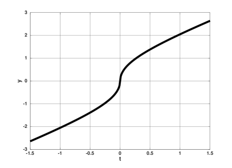
Figure 8: Null radial geodesic for the stealth defect (A.1) with metric functions (A.7), using dimensionless coordinates $y$ and $t$.

For a nonradial geodesic, the solutions of (A.5) are

$$\pm x = \frac{1}{4}\left((4-D)\arctan(\sqrt{D\,w-1})-\frac{\sqrt{D\,w-1}}{w}\right)+\widetilde{x}_{4}\,,$$ (A.9a)

with the definition

$$D \equiv \frac{\widetilde{E}+1/3}{\widetilde{J}^{\,2}}$$ (A.9b)

and a real constant $\widetilde{x}_{4}$.

For geodesics that do not cross the defect surface, we can, just as in Sec. 4.1, calculate the change in $x$,

$$\Delta x\equiv|x(y_{1})-x(\infty)|=\frac{\pi}{2}\left(1-\frac{1/4}{1+y_{1}^{2}}\right)\,,$$ (A.10)

where $y_{1}$ corresponds to the point on the line closest to the defect surface. For small $y_{1}$ (i.e., the line coming close to the defect surface), (A.10) shows that the line is bent away from the defect surface. This agrees with the fact that the effective mass near the defect surface is negative; see the $l(w)$ panel in Fig. 4 of Ref. 3.

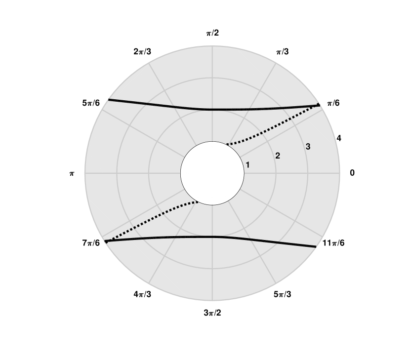
Figure 9: Geodesics in polar-type coordinates $(\sqrt{w},\,\phi)$, where the geodesics are given by (A.12). With the chart-2 coordinates $x$ and $y$, the azimuthal angle $\phi$ is defined by $\phi=x$ if $y>0$ and $\phi=x+\pi$ if $y<0$. The defect surface is given by the circle $w=1$ and part of the 3-dimensional space manifold (A.1), with metric functions (A.7), is indicated by the shaded area. The solid lines have constants $D=0.25$ and $x_{4}=\pi/2$ and the dotted-line segments have constants $D=1.25$ and $x_{4}=\pi/2$. The points on the solid lines which are closest to the defect surface have polar-type coordinates $(2,\,\pi/2)$ and $(2,\,3\pi/2)$, corresponding to the original coordinates $(y,\,x)=(\pm\sqrt{3},\,\pi/2)$.

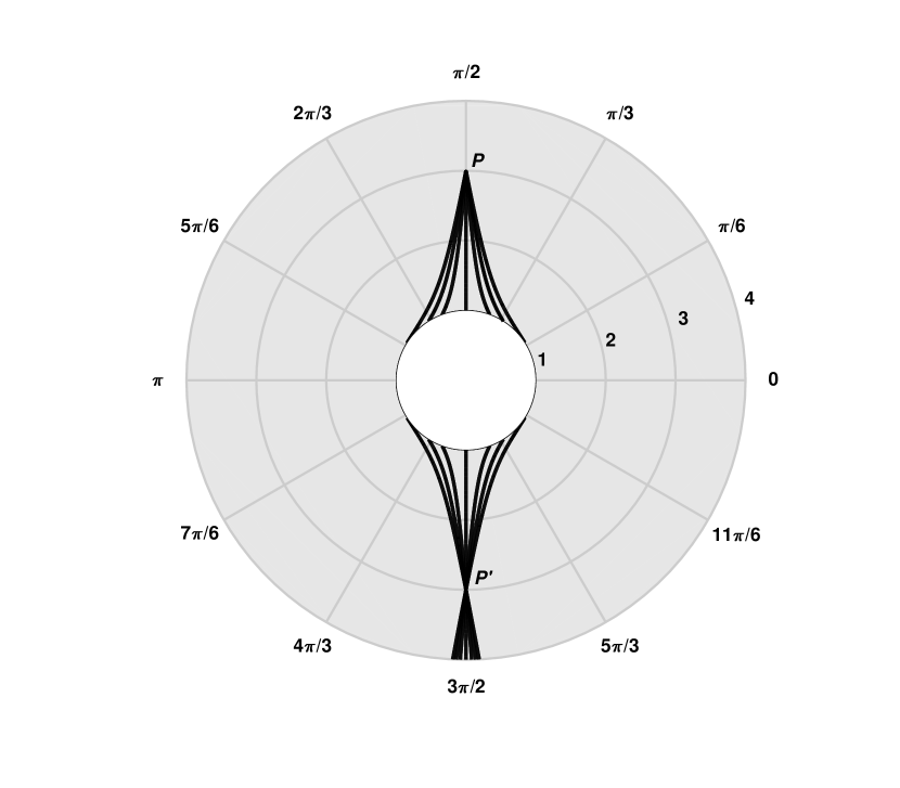
Figure 10: Family of geodesics in polar-type coordinates $(\sqrt{w},\,\phi)$, where the geodesics are given by (A.11) with plus signs on the left-hand sides. The defect surface is given by the circle $w=1$. The parameters of the six curved geodesics in the upper half-plane are, from left to right, ($D=1,\leavevmode\nobreak\ x_{4}=2.57258$), ($D=1.2,\leavevmode\nobreak\ x_{4}=2.5408766$), ($D=1.5,\leavevmode\nobreak\ x_{4}=2.4784766$), ($D=1.5,\leavevmode\nobreak\ x_{5}=\pi-2.4784766$), ($D=1.2,\leavevmode\nobreak\ x_{5}=\pi-2.5408766$), and ($D=1,\leavevmode\nobreak\ x_{5}=\pi-2.57258$). In terms of the original $(y,\,x)$ coordinates, the focal points $P$ and $P^{\prime}$ are given by $(y,\,x)_{P}=(\sqrt{8},\,\pi/2)$ and $(y,\,x)_{P^{\prime}}=(-\sqrt{8},\,\pi/2$).

Note that (A.9) can be rewritten in the following way:

$$\pm\frac{1}{\sqrt{D}} = \sqrt{w}\,\cos\left[\frac{4(x-x_{4})+\sqrt{D\,w-1}/w}{4-D}\right]\,,$$ (A.11a)

$$\pm\frac{1}{\sqrt{D}} = \sqrt{w}\,\cos\left[\frac{4(-x+x_{5})+\sqrt{D\,w-1}/w}{4-D}\right]\,,$$ (A.11b)

with real constants $x_{4}$ and $x_{5}$. As a concrete example, we first consider the solution corresponding to the upper sign on the left-hand side of (A.11a), that is,

$$\frac{1}{\sqrt{D}}=\sqrt{w}\,\cos\left[\frac{4(x-x_{4})+\sqrt{D\,w-1}/w}{4-D}\right].$$ (A.12)

For given values of $D$ and $x_{4}$, the solution (A.12) has, in general, two branches: one branch lies in the upper half-plane ($y>0$) and the other in the lower half-plane ($y<0$). The solid lines in Fig. 9 correspond to the orbits of two different particles, while the dotted line corresponds to the orbit of a third particle. Even though the points on the solid lines which are closest to the defect surface have $x=\pi/2$, these solid lines are not symmetrical about the line $x=\pi/2$ for $w\sim 2$, as can be verified in (A.12) with $x^{\prime}=\pi-x$ and $w(x^{\prime})\neq w(x)$.

In Fig. 10, finally, we give a family of geodesics in order to illustrate the lensing property of the curved-spacetime defect (cf. Fig. 7 for the lensing of the flat-spacetime defect). Apparently, the spherical symmetry of the metric is the crucial input for the lensing behavior.

References

- [1] F.R. Klinkhamer, “Skyrmion spacetime defect,” Phys. Rev. D 90, 024007 (2014), arXiv:1402.7048.
- [2] F.R. Klinkhamer and J.M. Queiruga, “Antigravity from a spacetime defect,” Phys. Rev. D 97, 124047 (2018), arXiv:1803.09736.
- [3] F.R. Klinkhamer and J.M. Queiruga, “A stealth defect of spacetime,” Mod. Phys. Lett. A 33, 1850127 (2018), arXiv:1805.04091.
- [4] F.R. Klinkhamer, “A new type of nonsingular black-hole solution in general relativity,” Mod. Phys. Lett. A 29, 1430018 (2014), arXiv:1309.7011.
- [5] F.R. Klinkhamer and F. Sorba, “Comparison of spacetime defects which are homeomorphic but not diffeomorphic,” J. Math. Phys. 55, 112503 (2014), arXiv:1404.2901.
-
[6]
M. Guenther,
“Skyrmion spacetime defect, degenerate metric,
and negative gravitational mass,”
Master Thesis, KIT, September 2017;
available from
https://www.itp.kit.edu/en/publications/diploma - [7] S. Weinberg, Gravitation and Cosmology: Principles and Applications of the General Theory of Relativity (Wiley & Sons, New York, 1972).
- [8] R.P. Feynman, R.B. Leighton, and M. Sands, The Feynman Lectures on Physics, Volume I (Addison–Wesley, Reading MA, USA, 1963).
- [9] P. Mouroulis and J. Macdonald, Geometrical Optics and Optical Design (Oxford University Press, New York, 1997).
- [10] A. Einstein, “Lens-like action of a star by the deviation of light in the gravitational field,” Science 84, 506 (1936).
- [11] K.S. Virbhadra and G.F.R. Ellis, “Schwarzschild black hole lensing,” Phys. Rev. D 62, 084003 (2000), arXiv:astro-ph/9904193.
- [12] V. Perlick, “On the exact gravitational lens equation in spherically symmetric and static space-times,” Phys. Rev. D 69, 064017 (2004), arXiv:gr-qc/0307072.
- [13] P. Schneider, J. Ehlers, and E.E. Falco, Gravitational Lenses (Springer-Verlag, Berlin, 1992).
- [14] J. Wambsganss, “Gravitational lensing in astronomy,” Living Rev. Rel. 1, 12 (1998), arXiv:astro-ph/9812021.
- [15] S. Dodelson, Gravitational Lensing (Cambridge University Press, Cambridge, England, 2017).
- [16] A. Shatskiy, “Einstein–Rosen bridges and the characteristic properties of gravitational lensing by them,” Astron. Rep. 48, 7 (2004), arXiv:astro-ph/0407222.
- [17] K.K. Nandi, Y.Z. Zhang, and A.V. Zakharov, “Gravitational lensing by wormholes,” Phys. Rev. D 74, 024020 (2006), arXiv:gr-qc/0602062.
- [18] R. Shaikh and S. Kar, “Gravitational lensing by scalar-tensor wormholes and the energy conditions,” Phys. Rev. D 96, 044037 (2017), arXiv:1705.11008.
- [19] S. Bernadotte and F.R. Klinkhamer, “Bounds on length-scales of classical spacetime foam models,” Phys. Rev. D 75, 024028 (2007), arXiv:hep-ph/0610216.
- [20] F.R. Klinkhamer and M. Schreck, “New two-sided bound on the isotropic Lorentz-violating parameter of modified-Maxwell theory,” Phys. Rev. D 78, 085026 (2008), arXiv:0809.3217.
- [21] F.R. Klinkhamer and J.M. Queiruga, “Mass generation by a Lorentz-invariant gas of spacetime defects,” Phys. Rev. D 96, 076007 (2017), arXiv:1703.10585.