The z=0.54 LoBAL Quasar SDSS J085053.12+445122.5: I. Spectral Synthesis Analysis Reveals a Massive Outflow

Abstract

We introduce SimBAL, a novel spectral-synthesis procedure that uses large grids of ionic column densities generated by the photoionization code Cloudy and a Bayesian model calibration to forward-model broad absorption line quasar spectra. We used SimBAL to analyze the HST COS spectrum of the low-redshift BALQ SDSS J085053.12+445122.5. SimBAL analysis yielded velocity-resolved information about the physical conditions of the absorbing gas. We found that the ionization parameter and column density increase, and the covering fraction decreases as a function of velocity. The total log column density is 22.9 (22.4) [$\rm cm^{-2}$] for solar ($Z=3Z_{\odot}$) metallicity. The outflow lies 1–3 parsecs from the central engine, consistent with the estimated location of the torus. The mass outflow rate is 17–$28\rm\,M_{\odot}yr^{-1}$, the momentum flux is consistent with $L_{Bol}/c$, and the ratio of the kinematic to bolometric luminosity is 0.8–0.9%. The outflow velocity is similar to the escape velocity at the absorber’s location, and force multiplier analysis indicates that part of the outflow could originate in resonance-line driving. The location near the torus suggests that dust scattering may play a role in the acceleration, although the lack of reddening in this UV-selected object indictes a relatively dust-free line of sight. The low accretion rate ($0.06L_{\rm Edd}$) and compact outflow suggests that SDSS J0850$+$4451 might be a quasar past its era of feedback, although since its mass outflow is about 8 times the accretion rate, the wind is likely integral to the accretion physics of the central engine.

1 Introduction

The optical and UV spectra of active galactic nuclei (AGN) and quasars offer powerful diagnostics of the physical conditions of gas in the vicinity of their central engines. Powered by photoionization, the broad emission lines trace the kinematics of the broad line region, likely dominated by Keplerian motions, while the broad absorption lines trace the outflow. A range of ionization states are seen from a number of different ground- and excited-state transitions. The broad emission lines are significantly Doppler-broadened by the motion of the gas in the vicinity of the black hole, with characteristic velocity widths of 1000s of $\rm km\,s^{-1}$, making line blending a considerable impediment to quantitative analysis. Emission-line studies are further compromised by the potential contributions to a single line from gas with a wide range of illumination patterns (e.g., the illuminated side of a cloud will emit differently than the back side of the cloud). Absorption line studies are more straightforward because only line-of-sight gas is important. Diagnostic power is lost when lines are saturated and complicated by the fact that the gas is known to partially cover the accretion disk, the source of the continuum emission. While we know that the gas must be clumpy in order to be dense enough to produce the emission and absorption that we see, there is no clear understanding of the characteristic scale and distribution of these clumps, or of how they are formed and maintained within the dynamic environment of the central engine.

Nevertheless, emission and absorption lines in quasars provide insight into fundamentally important phenomena. The central engine of quasars is not only a bright beacon in the Universe, exhibiting a rich phenomenology, but it also may be contributing to regulating the rate of star formation in the host galaxy (e.g., King & Pounds, 2015), thus contributing to the observed tight correlation between black hole mass and the mass of the bulge (e.g., Ferrarese & Merritt, 2000; Kormendy & Ho, 2013). Blue-shifted absorption lines, in particular, provide strong evidence for powerful outflows, and may prove to be key tracers of how accretion power may couple to the host galaxy’s interstellar medium.

Early quantitative analysis of broad absorption line quasar spectra focused on estimating the physical conditions of the gas, including ionization parameter, column density, and metallicity as a way of understanding the acceleration mechanism and potential for chemical enrichment of the intergalactic medium. Initially, these investigations proceeded with little concern for the width of the absorption lines. Arav et al. (2001) reported the analysis of the low-redshift quasar PG 0946$+$301, which has a FWHM of the main C IV component of about $8000\rm\,km\,s^{-1}$. Once partial covering was discovered to be important, investigators started working on determining the covering fraction and nature of partial covering (e.g., Hamann et al., 2001; de Kool et al., 2002c). Around the same time, scientists began to appreciate the diagnostic power of absorption lines with easily-populated excited states for determining the density of the outflows (e.g., de Kool et al., 2001, 2002a, 2002b). An issue is that many of the diagnostic pairs of lines (e.g., C II at 1334.0 and 1335.7 Å, S IV at 1062.7 and 1073.0 Å) lie quite close together in wavelength (e.g., Lucy et al., 2014, Fig. 15), making blending a problem for lines that are broad.

The focus on using excited states to determine the outflow density, and the accompanying problems with blending, means that much of the recent work to determine the physical conditions of the outflowing gas using spectroscopic diagnostics has been done on objects with relatively narrow lines. For example, HE 0238$-$1904 has several components with velocity widths of $500\rm\,km\,s^{-1}$ (Arav et al., 2013). FBQS J0209$-$0438 shows an absorption system with overall width of $600\rm\,km\,s^{-1}$ (Finn et al., 2014). QSO 2359$-$1241 shows Fe II absorption from various velocity components ranging in width from $<50\rm\,km\,s^{-1}$ to $\sim 100\rm\,km\,s^{-1}$ (Bautista et al., 2010). SDSS J1106$+$1939 shows S IV absorption with width of $\sim 2900\rm\,km\,s^{-1}$, while SDSS J1512$+$1119 shows S IV absorption with width of $\sim 250\rm\,km\,s^{-1}$ (Borguet et al., 2013). Yet the population of BAL quasars shows an enormous range of velocity widths. Baskin et al. (2015) report analysis of the C IV line from 1596 BAL quasars taken from the SDSS DR7 quasar catalog (Shen et al., 2011). The distribution of C IV width peaks at around $2000\rm\,km\,s^{-1}$ with a long tail to larger velocities. A cumulative distribution shows that 25% have velocity widths larger than $5200\rm\,km\,s^{-1}$, while 10% have velocity widths larger than $7500\rm\,km\,s^{-1}$. Limiting analysis to objects with narrow lines, or selecting out exactly those quasars with the strongest winds that are most likely to be important for feedback, may limit our understanding of quasar outflows.

Another issue was revealed by Lucy et al. (2014). In that paper, we analyzed the iron low-ionization broad absorption line quasar (FeLoBAL) FBQS J1151$+$3822. We modeled the lines using a normalized absorption-line template developed from the He I* absorption lines (Leighly et al., 2011). Following the procedure in the literature that has been used by many authors (e.g., Moe et al., 2009; Dunn et al., 2010; Borguet et al., 2012; Arav et al., 2013; Chamberlain et al., 2015), we fit the template to the spectrum in order to estimate the apparent column densities of line complexes. We compared the measured column densities with column densities predicted by the photoionization code Cloudy (Ferland et al., 2013), and used a figure of merit to determine the best-fitting values of ionization parameter $\log U$, density, and column density (parameterized as $\log N_{H}-\log U$). Our next step was novel. To check our best-fit result, we created a synthetic spectrum using the best-fitting parameters and overlaid it on the observed spectrum (Fig. 3b, Lucy et al., 2014). The resulting fit was a very poor match to the observed spectrum, potentially implying that the physical parameters derived using this type of analysis may be wrong.

Clearly a new approach is necessary, and we can take inspiration from work with other energetic systems. Supernovae are another type of astronomical object with broad absorption lines. In these objects, the lines can be so broad that identification of a feature can be difficult. Spectral synthesis codes have proven invaluable for both line identification (SYNOW, Branch et al., 2005) and for analysis of the physical conditions in the outflow (PHOENIX, Hauschildt & Baron, 1999). It stands to reason that a similar approach may be useful for broad absorption line quasars.

To that end, we introduce SimBAL, a spectral-synthesis forward-modeling method for analyzing BAL quasar spectra. SimBAL, in essence, inverts the conventional method for analyzing absorption lines. Instead of fitting individual lines and then comparing those measurements with Cloudy models, synthetic spectra are constructed from Cloudy models and then compared with the observed spectrum. The spectral synthesis approach has several advantages. First, because we do not need to identify individual absorption lines, blending is not an issue, so the width of the line no longer is an impediment to selection of quasars for analysis. Second, the conventional analysis method outlined above focuses on the lines that are observed, neglecting the important information provided by lines that are not detected. Since the spectral synthesis approach models the whole spectrum, the information provided by absent lines is used to constrain the solution. Finally, we use a Markov Chain Monte Carlo method in physical parameter space to compare the synthetic spectrum with the observed spectrum. This method allows us to harvest uncertainties on the physical parameters from the posterior probability distributions. Along the way, we have also discovered that we can map the physical parameters of the outflow (e.g., ionization parameter, column density, and covering fraction) as a function of velocity, properties that may be important for constraining acceleration models for the outflows. With the physical properties of the outflow in hand and a few assumptions, we can estimate mass outflow rates, key for constraining the kinetic energy available for quasar feedback on the host galaxy.

In this paper, we use SimBAL to analyze HST COS spectrum of the low redshift ($z=0.5422$) LoBAL quasar SDSS J085053.12$+$445122.5, hereafter referred to as SDSS J0850+4451. The observation and continuum model are described in §2. A brief description of SimBAL is given in §3. The absorption modeling and extraction of the physical parameters of the outflow is described in §4. The implications of our analysis are discussed in §5, the summary of our principal results and future development of SimBAL are discussed in §6, and several potential systematic effects are discussed in an Appendix. Vacuum wavelengths are used throughout. Cosmological parameters used depend on the context (e.g., when comparing with results from an older paper), and are reported in the text.

2 Observations and Data Reduction

2.1 HST COS Observations

SDSS J0850$+$4451 was observed with HST COS (Osterman et al., 2011) using the G230L grating on 2013 May 12. The goal of the observation was to obtain high signal-to-noise spectra covering the major broad absorption lines including P V$\lambda\lambda 1118,1128$ on the short wavelength end and C IV on the long wavelength end. Two central wavelengths were used. The 33,971-second exposure using the 2950Å setting provided rest-frame coverage from 1080 to 1380Å. The 8,848-second exposure using the 3360Å setting provided rest-frame coverage between 1370 and 1640Å. The “x1dsum” spectra were extracted from the pipeline fits files.

The spectrum was corrected for Milky Way reddening using $E(B-V)=0.024$ (Schlafly & Finkbeiner, 2011). The spectrum was shifted to the rest frame using a cosmological redshift of $0.5422$. This value was estimated from the narrow [O III] line in the SDSS spectrum, and is between 0.5423, the value determined by Hewett & Wild (2010), and 0.5414, the NED preferred redshift.

2.2 Continuum Model

The HST spectrum shows rather prominent UV emission lines typical of a broad-line AGN. The spectrum appears to be similar to the LBQS quasar composite spectrum (Francis et al., 1991). Leighly (2004) showed that a range of C IV profiles can be modeled using an intermediate-width component at approximately the rest wavelength and a broad and blueshifted component, with variable flux ratio between the two components. We first developed a model of the LBQS quasar composite C IV line. This line is somewhat broad and slightly blueshifted, and could be fit well with two Gaussians, one with a width of $9800\rm\,km\,s^{-1}$ and larger blue offset $-1520\rm\,km\,s^{-1}$, and the other with a width of $3750\rm\,km\,s^{-1}$ and smaller blue offset of $-285\rm\,km\,s^{-1}$. Our model for SDSS J0850$+$4451 consisted of two Gaussians with the same offsets and widths as the LBQS C IV model, but variable flux ratio. We used this emission line profile model to model C IV, Si IV, N V, Ly$\alpha$, and Si II$\lambda 1264$, constraining the flux ratio between the two components to be equal for the doublets. The underlying continuum could be modeled adequately using a broken power law, but a 4th-order polynomial provided a better fit. The best-fitting model and data are shown in Fig. 1. The statistical uncertainty in the spectrum is also shown to highlight the fact that the signal-to-noise ratio in this spectrum is low for the shortest wavelengths that cover the diagnostically important P V line. Henceforth, this continuum model is referred to as the “first continuum model”.

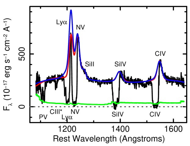
Figure 1: The HST far-UV spectrum (black) and continuum models. The red line shows the model referred to as the “first continuum” in the text, obtained assuming that the feature near 1212Å is unabsorbed continuum plus line emission. The blue line shows the model referred to as the “second continuum”, obtained assuming that the Ly$\alpha$ emission line is partially absorbed. Principal emission lines are labeled above the spectrum, and principal absorption lines are labeled below. See text for details. The statistical uncertainty in the spectrum is shown in green. The mean signal to noise ratio in the spectrum was 7.2, dropping to 2.2 shortward of $\sim 1100$ Å.

While this model provided a good fit over the whole bandpass, some ambiguity remains. Our solution assumes that the prominent feature near 1212Å is unabsorbed continuum and line emission. However, that feature may be partially absorbed continuum and line emission instead, since in our first continuum model (shown in red in the figure), the contribution by N V is larger than the contribution from Ly$\alpha$. We created another continuum estimate by first fitting the mean model spectrum obtained by Pâris et al. (2011) from a sample of $z\sim 3$ SDSS quasars with the model outlined above, and then requiring the ratio of the intensity of Ly$\alpha$ to C IV in our spectrum to be equal to the one obtained from the mean $z\sim 3$ spectrum. This model left us with a significant contribution from N V emission which is well constrained on the red side of the line. The N V emission line could be enhanced in BALQs by resonance scattering of Ly$\alpha$ (Wang et al., 2010; Hamann & Korista, 1996). This model is referred to as the “second continuum model”.

One of the uncertainties in modeling broad absorption line quasars is the placement of the continuum. In SDSS J0850$+$4451, there is enough visible continuum between absorption lines that the only region of significant uncertainty is in the vicinity of Ly$\alpha$, which we account for as discussed above. We are currently developing a technique that models the continuum simultaneously with the absorption lines (Marrs et al., 2017; Wagner et al., 2017; Leighly et al., 2017). In any case, SDSS J0850$+$4451 has deep lines, so continuum placement is relatively less important for this object than for objects with shallow lines, where there is little contrast between the absorption lines and the continuum.

3 SimBAL

We provide a brief overview of the SimBAL analysis method. Our model column densities are computed using the photoionization code Cloudy (Ferland et al., 2013). This mature code is well documented and maintained, and has a large, constantly updated atomic library. For this paper, we use data produced by version C13.03 of the code. A number of input parameters are required. For the spectral energy distribution (SED) of the light illuminating the slab of gas, we began with a relatively soft SED that may be characteristic of quasar-luminosity ($\gtrsim 10^{46}\rm\,erg\,s^{-1}$) objects (Hamann et al., 2013). To check for systematic uncertainty associated with SED choice, we also use a relatively hard SED (Korista et al., 1997) that may be more appropriate for Seyfert galaxies ($\lesssim 10^{45}\rm\,erg\,s^{-1}$). Our baseline abundances are the default solar abundances (see the Cloudy manual Hazy for references). To investigate systematic uncertainty associated with abundances, we also ran a set of simulations with $Z=3Z_{\odot}$, i.e., all the metals have abundances three times the solar value, with nitrogen enhanced by a factor of $Z^{2}$, and helium enhanced by a factor of 1.14 (Hamann et al., 2002). Other potential systematic uncertainties and model dependencies are discussed briefly in Appendix A.

The physical conditions of the gas are parameterized using the dimensionless ionization parameter $\log U$, the gas density $\log n\rm\,[cm^{-3}]$, and a combination parameter $\log N_{H}-\log U$ which essentially measures the column density of the gas slab with respect to the hydrogen ionization front, usually near 23.2 in this parameterization and depending on the spectral energy distribution. Depending on the application, our calculational grid spans $-4.0<\log U<2$, $2.8<\log n<9$, and $21.5<\log N_{H}-\log U<23.7$ with grid spacing 0.05, 0.2, and 0.02, respectively. The broad absorption lines in SDSS J0850+4451 have a low minimum velocity, and C IV line is deep and nearly black. This indicates that the broad line region is covered, and therefore the absorber is outside of the broad line region. Therefore, a maximum density of $n=10^{9}\rm\,cm^{-3}$ is a reasonable choice. The column densities $N(ion)$ of 179 ground and excited state atoms and ions were extracted from the output. These results were combined with our current line list which includes 6267 transitions. The result is a large file that is used as input to SimBAL, and from which we synthesize the spectra.

The opacity as a function of velocity can, in principle, have any functional form, or be specified by a template. For a single Gaussian opacity profile, there are six parameters required for the model. These include the three gas parameters discussed above ($\log U$, $\log n$, $\log N_{H}-\log U$). Also required are two parameters to describe the kinematics: the velocity offset $v_{\rm off}$ and the velocity width $v_{\sigma}$, both specified in $\rm km\,s^{-1}$, and one parameter to describe the covering fraction of the gas. While the partial covering can be parameterized in many ways (e.g., Sabra & Hamann, 2001), we choose power-law partial covering, where $\tau=\tau_{max}x^{a}$. In this parameterization, $\tau$ is the integrated opacity of the line, while $\tau_{max}$ is proportional to $\lambda f_{ik}N(ion)$, where $\lambda$ is the wavelength of the line, $f_{ik}$ is the oscillator strength, $N(ion)$ is the ionic column density (e.g., Savage & Sembach, 1991), and $x\in(0,1)$ represents the projection of the two-dimensional continuum source onto a normalized one dimension. The exponent on $x$ in the form $\log a$ is then the parameter that is modeled in the MCMC. The power-law partial covering model has been explored by de Kool et al. (2002c); Sabra & Hamann (2001); Arav et al. (2005), and sometimes it is found to provide a better fit than the step-function partial covering model (de Kool et al., 2002c; Arav et al., 2005). We choose this parameterization for the practical reason that because we build the synthetic absorption spectrum line by line, we need a parameterization that is mathematically commutative. The more commonly used step function covering fraction parameterization is not mathematically commutative. In addition, the power law parameterization naturally explains the observation that high-opacity lines are observed to have a larger covering fraction than low-opacity lines (e.g., Hamann et al., 2001).

In the power-law covering fraction parameterization, the fraction of the source covered, or alternatively, the residual intensity, depends on the total opacity of the line. Therefore, in a photoionized gas, where the opacity of different lines can differ dramatically, so can the residual intensity. The width of the line is important, because one observes $d\tau/dv$, and therefore a wide line will be less optically thick than a narrow line for the same total ionic column density. For reference, the average optical depth of a line in this parameterization is $\bar{\tau}=\int_{0}^{1}\tau_{max}x^{a}=\tau_{max}/(1+a)$. Arav et al. (2005) pointed out that for $\tau(x)=\tau_{max}x^{a}$, the x-value for which $\tau(x)$ becomes greater than 0.5 provides a good estimate of the residual intensity in the line.

Once the choice of input Cloudy matrix and opacity model has been made, the spectral synthesis modeling can be done. The synthetic spectrum is created during the simulations on rest frame wavelengths of the spectrum to be modeled. The synthetic spectrum is compared with the observed spectrum using a likelihood based on $\chi^{2}$. Markov Chain Monte Carlo allows efficient exploration of parameter space. We use the emcee code (Foreman-Mackey et al., 2013), which uses the Goodman & Weare (2010) affine invariant MCMC sampler. This method has the advantage that it can efficiently build up a posterior probability distribution even in the face of highly correlated parameters. Our model requires specification of a prior whose minimal constraints keep the model parameters within the computational boundaries. We used flat priors for the physical parameters of the gas, to ensure that the solution stays within the computed Cloudy model grid. We used Gaussian priors for the line offsets and widths, based on inspection, and we checked that the posteriors of these parameters were always narrower than the priors. The code produces a chain of values, which, after a period of burnin, can be used to construct the posterior probability distributions of the free parameters, or properties derived from them (e.g., the best-fitting model spectrum, or derived quantities such as the mass accretion rate). For this application, we typically do 20,000 simulations using 300 walkers on $\sim 25$ double-threaded cores. A flow chart of the procedure is shown in Fig. 2.

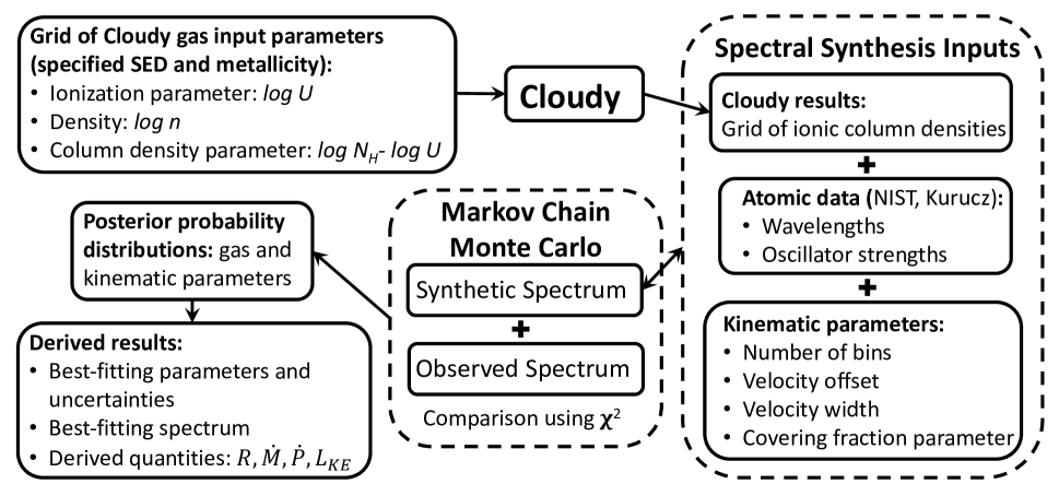
Figure 2: A flow chart illustrating the SimBAL analysis procedure. Cloudy models are calculated in advance on an array of ionization parameter ($\log U$), density ($\log n$), and a combination column density parameter ($\log N_{H}-\log U$) to yield a grid of ionic column densities. Combined with atomic data and kinematic parameters including the velocity offset, velocity width, and covering fraction parameter, synthetic spectra are generated in real time. Using a Markov Chain Monte Carlo solver, the synthetic spectra are compared with the observed spectrum using a likelihood based on $\chi^{2}$. The output is a chain of values mapping the posterior probability distribution of the modeled parameters, from which results such as the best-fitting spectrum can be constructed.

4 Absorption-Line Modeling

4.1 Single Gaussian Opacity Profile

In this section, we present the SimBAL models of the HST spectrum. To demonstrate the need for a complex model, we began by using a single Gaussian opacity profile (e.g., Borguet et al., 2012; Moravec et al., 2017), and performed the MCMC modeling as outlined above. From the results we constructed the median and 95% confidence spectra. These are shown in Fig. 3.

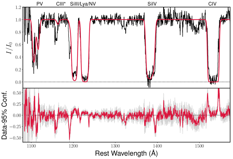
Figure 3: The results from a single Gaussian profile model fit to the HST spectrum. In the top panel, the median synthetic spectrum (crimson) is overlaid on the continuum-normalized spectrum (black). The lower panel shows the spectrum minus the median model and errors in gray, and the filled region between the spectrum and plus and minus the 95% confidence synthetic spectra in crimson, respectively. Significant negative and positive residuals are observed, indicating that the spectrum cannot be adequately modeled using a single Gaussian opacity profile.

The figure shows that while the character of the bulk of the absorption is captured by the single Gaussian model, the absorption is not modeled well in detail. Neither the C III*$\lambda 1175$ feature observed near 1160Å nor the Si III$\lambda 1206$ observed near 1190Å is modeled well. In addition, the C IV absorption line appears too broad compared with e.g., Si IV; this occurred because the C IV line is optically thick, resulting in significant opacity in the wings of the lines, while the Si IV is less saturated.

We compute reduced $\chi^{2}$ for our models as follows. We desire to determine the goodness of fit of the absorption model. We model the continuum ahead of time, and therefore the regions of the model spectrum that have the value of 1 cannot contribute to determining the goodness of fit. So we exclude those regions from our computation of $\chi^{2}$. The reduced $\chi^{2}$ for this model is 2.76. Note that we distinguish these measurements of $\chi^{2}$ from the likelihood used in the MCMC (above). There, the lack of the line is important for constraining models, so we use the full wavelength range.

4.2 Accordion Models

From the shape of the absorption lines and residuals shown in Fig. 3, it is clear that the spectrum can only be explained adequately with multiple absorbing components. An obvious next choice is a model consisting of multiple Gaussians. A problem with multiple Gaussians with all parameters free is that they can move enough in the spectral fitting to mix with one another in the MCMC. We found that a constrained multicomponent model is more robust in the spectral fitting, and has the added benefit of yielding information about the physical conditions as a function of velocity.

We call the constrained model that we used an “accordion model”. The model is characterized by multiple components that we call “bins” to emphasize that these are not to be considered separate velocity components in the outflow, but rather a parameterization of the opacity as a function of velocity. Each bin has the same width and separation from its neighbors in velocity space. The fitting parameters are then the maximum velocity offset (i.e., the central velocity of the shortest-wavelength bin), the velocity width of the bins, the separation of the bins (3 parameters), and, most generally, $\log U$, $\log n$, and $\log N_{H}-\log U$ for each bin ($3x$ the number of bins). We tried two versions of the accordion model: one used a Gaussian bin, and the other used a tophat bin. The tophat accordion model had one fewer parameter than the Gaussian accordion model because the width of a bin is equal to the separation.

We rejected the Gaussian accordion model for the following reasons. In the tophat accordion model, the opacity of each bin is independent of its neighbors; this is by construction. To put it another way, there is no blending of adjacent bins. Therefore, in a tophat accordion model, for a feature comprised of a single transition, a plot of the individual bins will touch the minimum flux points of the synthesized spectrum and therefore follow the outline of the feature smoothly (except for the stepped approximation). In contrast, the opacity of bins are not independent in the Gaussian accordion model, because the wings of adjacent Gaussian bins must overlap, even if the individual bins are narrow. So in a corresponding plot of individual bins for the Gaussian accordion model, the minimum values of the individual bins will not touch the minimum flux level of the synthetic model spectrum; they all appear optically thinner (or appear to have a lower covering fraction) than the feature does (e.g., Rupke et al., 2002, Fig. 11). We suggest that this lack of independence results in unreliable inferences about the wind properties for the main features of the absorption, although there is evidence that the Gaussian accordion model can pick up low covering fraction features with different properties (e.g., $\log U$ or $\log N_{H}-\log U$) but the same velocities as the main features. We therefore reject the Gaussian accordion model and only consider the tophat accordion model for the remainder of this paper.

We first present a tophat accordion model with 11 bins. In this model, the ionization parameter, column density parameter $\log N_{H}-\log U$, and covering fraction power-law index $\log a$ were allowed to vary freely for each bin. The density was allowed to have two values, depending on the bin, with the reasoning for that choice as follows. C III*$\lambda 1175$ is a transition from a metastable state (the decay from that state produces the C III]$\lambda 1909$ emission line). The level is complex, with $J=0$, $J=1$, $J=2$ states. These states have different transition probabilities and therefore have different critical densities (e.g., Gabel et al., 2005). These properties make the C III*$\lambda 1175$ is a density-sensitive line (see Arav et al., 2013, for a discussion of the utility of density-sensitive lines for determining absorber distances), but rarely used because the transitions are close together and cannot be deblended except for the narrowest of absorption lines (Gabel et al., 2005; Borguet et al., 2012). The spectral synthesis approach does not require deblending, so we can use this line to determine the density of the portion of the outflow (i.e., velocity range) represented by this line. For 11 bins, that range was the 4th, 5th, and 6th bins from the left (i.e., spanning $-3200$ to $-4450\rm\,km\,s^{-1}$). As shown below, this feature is characterized by a larger value of $\log N_{H}-\log U$, and we refer to this enhanced column density region in the outflow as the “concentration” henceforth. The densities of these three high-column-density bins were constrained to have the same value, and the densities of the remaining seven were constrained to have a different value. Thus, two values of density were fit.

The model and the difference between the data and the median spectrum for the second continuum model is shown in Fig. 4; the results for the first continuum model are very similar. The fits are very good overall. The reduced $\chi^{2}$ for this model and others discussed below are shown in Fig. 5. As discussed above, in order to ascertain goodness of fit of the absorption model, we compute the reduced $\chi^{2}$ over regions of the spectrum where the model absorption optical depth is greater than zero. For the typical number of degrees of freedom (around 500), a value of reduced $\chi^{2}$ greater than 1.2 is excluded at a 99% confidence level. Generally, the second continuum model produces a slightly better fit than the first continuum model.

There are several notable residuals. Just left of the C III* line at 1160 Å is a sharp line-like feature, which is plausibly a Ly$\alpha$ forest line, although some models fit this feature and some do not. Around 1320 Å are a pair of features that are consistent with C II$\lambda 1335$ at $v=-4120\rm\,km\,s^{-1}$ and $v=-2460\rm\,km\,s^{-1}$, i.e., within the velocity range of the main feature. C II is a low ionization line that appears at slightly larger values of $\log N_{H}-\log U$ that are represented in this object (see Fig. 10) Finally, there is a broad feature centered around $\sim 1490$ Å that probably originates in high-velocity gas, centered around $\sim-11200\pm 1300\rm\,km\,s^{-1}$ (1$\sigma$), that is of low optical depth so that only C⁺³ presents significant opacity. Ly$\alpha$ absorption from this feature is predicted to lie between 1166 and 1176Å, and there is no absorption observed in that band. Absorption from N V could plausibly be blended with the observed Si III$\lambda 1207$ / Ly$\alpha$ feature, but it is likely to be quite shallow if present. We ignore these features henceforth.

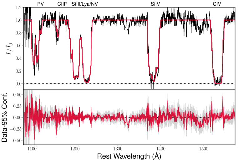
Figure 4: The results from an 11-bin tophat accordion model. In the top panel, the median synthetic spectrum (crimson) is overlaid on the continuum-normalized spectrum (black). The lower panel shows the spectrum minus the median model and errors in gray, and the filled region between the spectrum and plus and minus the 95% confidence synthetic spectra in crimson, respectively. Overall, the fit is good. Negative residuals near 1160, 1320, and 1490Å are plausibly an intervening Ly$\alpha$ forest line, C II characterizing slightly higher values of $\log N_{H}-\log U$ than are represented here, and C IV from a low-opacity high-velocity outflow, respectively.

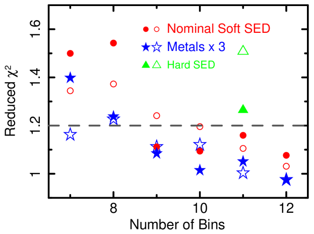
Figure 5: Reduced $\chi^{2}$ for the 26 tophat accordion models presented in this paper, evaluated between 1080Å and 1573Å as described in §4.1. In each case, the open symbols show the first continuum model, while the solid symbols show the second continuum model (see §2.2). Formally, values of reduced $\chi^{2}$ greater than $\sim 1.2$ (dashed line) are unacceptable at 99% confidence. We find that the larger the number of bins, the better the fit, the $Z=3Z_{\odot}$ metallicity provides a slightly better fit than solar metallicity, and the hard SED yields a relatively poorer fit than the soft SED.

Fig. 6 displays the individual velocity bins for the case of the second continuum model and $Z=3Z_{\odot}$ abundances (see § 4.2.3). The absorption as a function of velocity is shown, with a different color for each velocity bin. Individual members of the doublets can be distinguished in P V, N V, Si IV, and C IV. For this model, the width / separation of the bins is rather tightly constrained in order that the opacity for Ly$\alpha$ and N V meet to form the low-absorption region near 1212Å. It is also notable that the best-fitting bin width is such that the C IV doublet lines are in adjacent bins, while the Si IV doublet lines are separated by four bins. This result makes sense since the doublet separation for C IV is $492\rm\,km\,s^{-1}$, while the doublet separation Si IV is $1932\rm\,km\,s^{-1}$, i.e., 4 times larger.

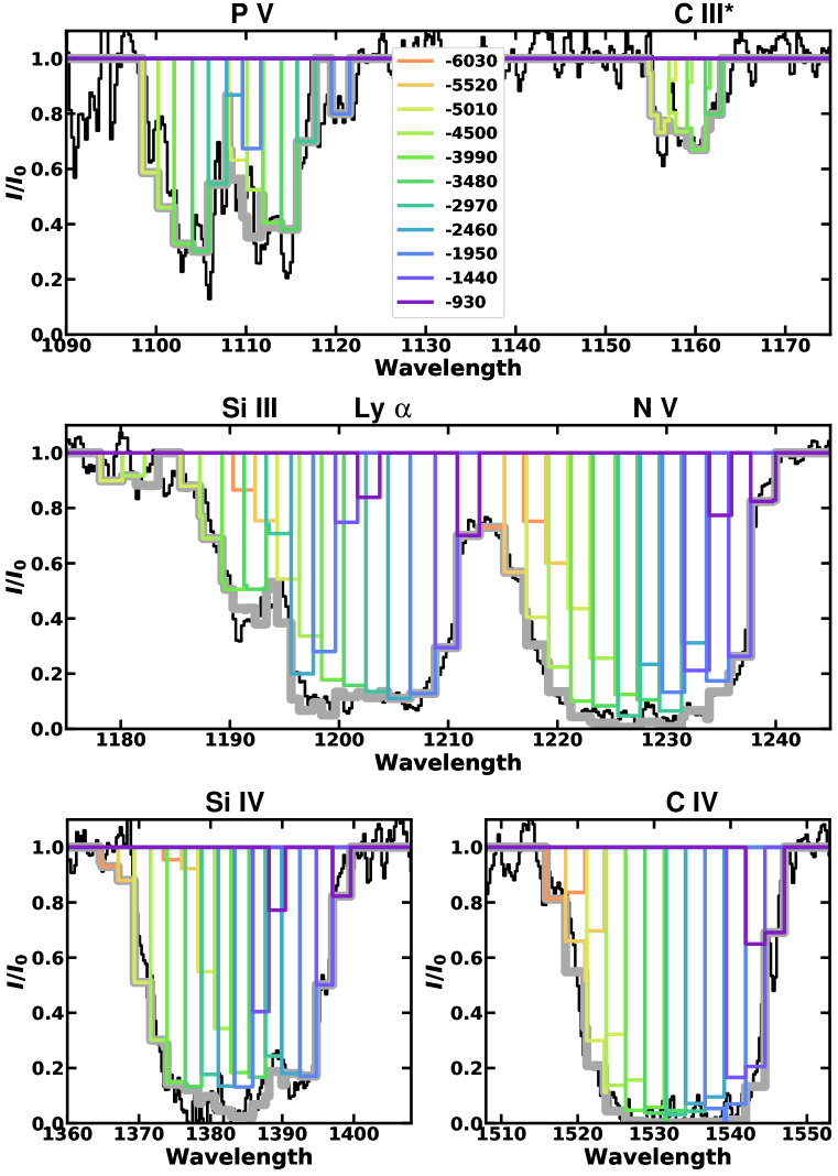
Figure 6: The results from an 11-bin tophat accordion model for the second continuum model and enhanced metallicity ($Z=3Z_{\odot}$); see § 4.2.3. Each of the bins is shown by a different color, and the full line profile is shown in a thick light gray line overlaid on the continuum-normalized data (black). The principal lines contributing to the opacity are identified over the features. The opacity for each member of the resonance doublets P V, N IV, Si IV, and C IV can be seen. The limited extent of the density-sensitive C III* line can be seen; only four of the eleven bins, with center velocities between $-5010\rm\,km\,s^{-1}$ and $-3480\rm\,km\,s^{-1}$, contribute this this line.

What is the effect of the number of bins? To investigate this point, we considered models with 7, 8, 9, 10, 11, and 12 bins. As above, the ionization parameter, $\log N_{H}-\log U$, and covering fraction $\log a$ were allowed to vary freely in each bin, and two densities were used. The number of bins spanning the concentration varied, generally increasing as the number of bins was increased and as each bin became narrower. The quality of the fit improved as the number of bins was increased, likely due to the greater flexibility of the model; the reduced $\chi^{2}$ in the 1080Å to 1573Å region as a function of the number of bins is shown in Fig. 5. As noted above, for the typical number of degrees of freedom, a value of reduced $\chi^{2}$ greater than 1.2 is excluded at 99% confidence level, suggesting that the 7- and 8-bin cases do not provide sufficient flexibility to model velocity dependence of the absorption profiles.

Fig. 7 shows the parameter constraints obtained from the posterior probability distributions (i.e., the MCMC chain excluding burnin) for all 6 number-of-bin combinations for the first continuum model, and Fig. 8 shows the same result for the second continuum model. In each case, the best-fitting point is the Maximum Amplitude Probability (MAP) of the posterior probability distribution, and the error bars are obtained from the 4.6% and 95.4% (i.e., $2\sigma$) points on the cumulative distribution. The results are shown for the four fitted parameters ($\log U$, $\log N_{H}-\log U$, covering fraction index $\log a$, and $\log n$). We also graph the column density $\log N_{H}$, weighted by the covering fraction, i.e., the amount of gas in the outflow, which is computed from the sum of $\log N_{H}-\log U$, $\log U$, and $\log(1.0/(1.0+a))$ at each point in the chain.

Several trends are apparent. The parameters are better constrained in the middle of the feature, where the absorption is deepest, compared with the wings. The ionization parameter shows a slight increase towards higher velocities and a dip near $-2500\rm\,km\,s^{-1}$. The column density parameter, $\log N_{H}-\log U$ is clearly higher by a factor of 3 in the vicinity of the concentration. The density is poorly constrained, even when only two values are used, but it is better constrained (by C III*) in the vicinity of the concentration as compared with the values outside the concentration.

The covering fraction parameter varies strongly with velocity, with a lower covering fraction at higher velocities. In the vicinity of the concentration, the covering fraction $\log a=0.5$, and at higher velocities, the covering fraction $\log a\sim 1$. The covering fraction is the most strongly variable parameter, indicating that it is important in determining the shapes of the troughs. The strong dependence on covering fraction is consistent with the behavior of other outflows, where the apparent optical depths of absorption lines are found to be controlled principally by covering fraction, rather than the ionic column density as one might expect (e.g., Arav, 2004, and references therein). Note that the covering fraction variations do not mirror the photoionization properties of the gas; for example, the covering fraction maximum, located around $-2500\rm\,km\,s^{-1}$, is not at the same velocity as the $\log N_{H}-\log U$ maximum, located between $-3200$ to $-4450\rm\,km\,s^{-1}$, i.e., the concentration.

The covering-fraction weighted column density is roughly constant for velocities faster than $-3300\rm\,km\,s^{-1}$, with an average column over that region of $\log N_{H}=22.0\rm\,[cm^{-2}]$. This region includes the concentration, between $-4400$ and $-3300\rm\,km\,s^{-1}$, which exhibits a distinctly greater value of $\log N_{H}-\log U$ (Fig. 4). But it also includes, interestingly, the highest velocity portions of the outflow, which have lower value of $\log N_{H}-\log U$ and a higher value of $\log a$ (corresponding to a lower covering fraction), which would tend to decrease the inferred column density. Those two factors are offset by a higher value of $\log U$ approaching 1, corresponding to a thicker H II region, which offsets the effects of the lower $\log N_{H}-\log U$ and higher $\log a$. The error bars are large, as the feature is shallow at the highest velocities, so this result is uncertain. The column density decreases at lower velocities, to an approximate constant level for velocities smaller than $-2800\rm\,km\,s^{-1}$, of $\log N_{H}=21.4\,\rm[cm^{-2}]$.

The ionization parameter and covering-fraction weighted column densities are both larger at high velocities and smaller at low velocities, suggesting a correlation between the ionization parameter and column density.

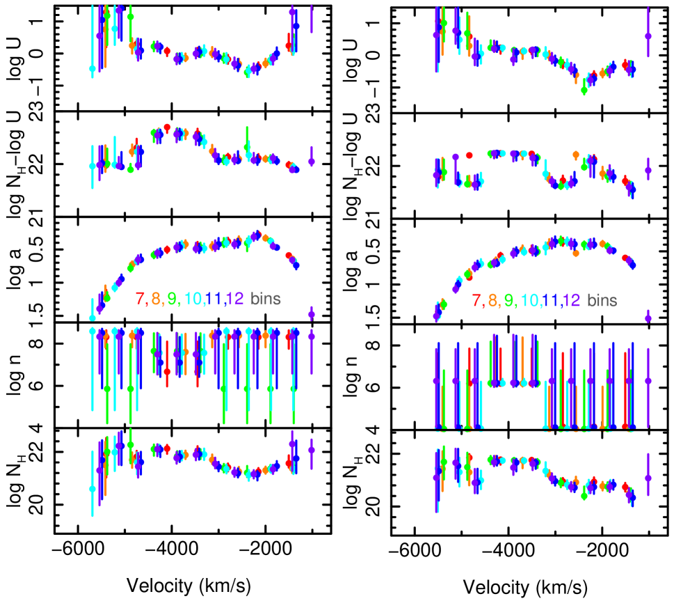
Figure 7: The spectral fitting results as a function of velocity offset for a range of number of bins spanning the absorption profile. The Maximum Amplitude Probability (MAP) values and 95% confidence regions from the posterior probability distributions are shown. The left (right) panel shows the results for solar ($Z=3Z\odot$) metallicity, both for the soft SED and the first continuum model. In each of the 12 models (six bin values and two metallicities), the ionization parameter $\log U$, the column density parameter $\log N_{H}-\log U$, and the covering fraction parameter $\log a$ were allowed to vary independently in each bin, while the density was allowed to take on one of two values depending on whether or not a bin was represented in the density-sensitive line C III*$\lambda 1175$ which spans the enhancement in $\log N_{H}-\log U$ between $-4500$ and $-3500\rm\,km\,s^{-1}$ (identified in the text as the concentration). As expected, the density is constrained only over the ranges of velocities where the C III*$\lambda 1175$ line is present. The column density parameter varies significantly as a function of velocity, being about a factor of three larger between $-4400$ and $-3200\rm\,km\,s^{-1}$, and the covering fraction decreases strongly as a function of velocity.

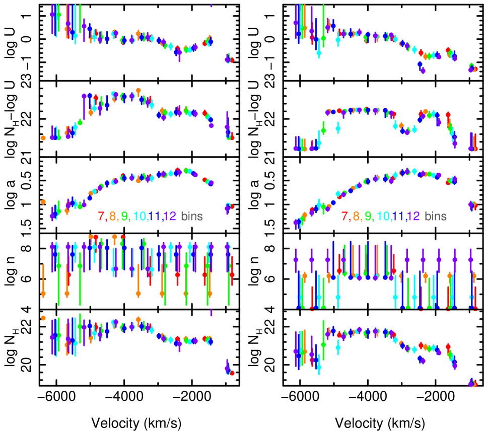
Figure 8: Same as Fig. 7, for the second continuum model. The principal differences lie at the lowest velocities and the highest velocities. The low-velocity end of the Ly$\alpha$ absorption and the high-velocity end of the N V absorption abut at the high point between these two features (see Fig. 6). This requirement has the effect of strongly constraining allowed values of velocity for the bins.

The results for the second continuum model are shown in Fig. 8. Overall, they are qualitatively similar. The differences principally originate in the requirement that some opacity, but not too much, be present on the boundary between the N V and Ly$\alpha$ lines, resulting in rather stringent constraints on the widths of the bins; this forced the whole feature to be wider for the second continuum, and to have lower opacity at the highest and lowest velocities. It is also responsible for the relatively poorer fits for the 7- and 8-bin models.

4.2.1 What Drives the Fits?

The MCMC results show relatively small uncertainties in the model parameters, with the exception of $\log n$, which is in general poorly constrained. In addition, some of the fit parameters vary as a function of velocity. It is therefore interesting to investigate what properties of the spectrum result in these well-fitting and relatively tightly-constrained models. We did this by isolating the best fit (median values from the posterior) and then varying one parameter while leaving the others fixed at the best value.

Fig. 9–12 show two still frames from each of the animations that are available online. In each figure, the red line shows the best fitting median model spectrum, while the blue line shows the model spectrum for minus and plus 0.5 dex from the best fit for each of the varied parameters (with the exception the plot for $\log n$, which is less sensitive to variation).

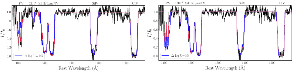
Figure 9: Varying parameters away from the best fit demonstrates that certain individual lines or groups of lines are responsible for the relatively well-constrained parameters obtained. The results (blue line) for varying the ionization parameter away from the best fit (red line) for the 11-bin tophat accordion model are shown, with the negative change in the left panel, and the positive change in the right panel. The figure shows that P V is principally responsible for constraining the ionization parameter. This figure is available as an animated movie online.

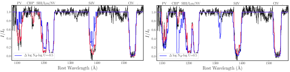
Figure 10: The same as Fig.  9 for $\log N_{H}-\log U$. The plot shows that correlated variability among several lines, especially C III* and Si IV, as well as lines that are not observed (such as C II$\lambda 1335$) are responsible for constraining $\log N_{H}-\log U$. This figure is available as an animated movie online.

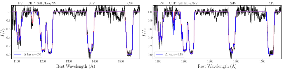
Figure 11: The same as Fig.  9 for covering fraction parameter $\log a$. Note that a larger value of $a$ corresponds to a lower covering fraction (see § 3). The plot shows that varying $\log a$ causes all lines to vary together. This figure is available as an animated movie online.

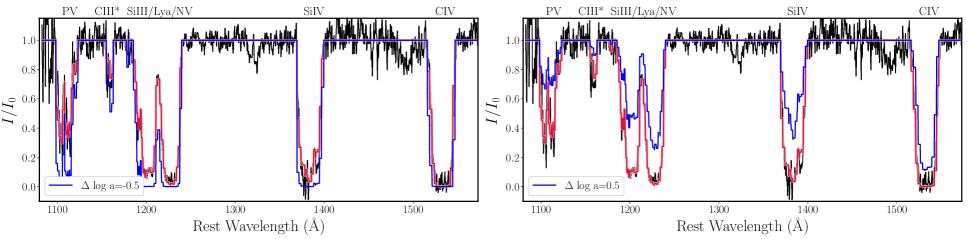
Figure 12: The same as Fig.  9 for the density $\log n$, with the exception that the log density is varied to $\Delta\log n=-2.0$ and $\Delta\log n=1.15$ to account for the lower sensitivity of the simulations to this parameter. Only C III* is sensitive to density in this bandpass. This figure is available as an animated movie online.

The simulation in Fig. 9 shows that it is the P V that constrains the ionization parameter in the vicinity of the best fit. Conventionally, P V is thought to be a diagnostic of column density, not ionization parameter (e.g., Hamann, 1998). Since phosphorus is a factor of 765 times lower in abundance than carbon, observation of a significant P V line implies a strongly saturated C IV line and a high column density (e.g., Leighly et al., 2009; Borguet et al., 2012). In addition, P⁺⁴ and C⁺³ are the dominant ionization state of their respective elements at nearly the same ionization parameter of about $\log U=-2$ (e.g., Hamann, 1997, Fig. 2). However, because of the low abundance of phosphorus at $\log U=-2$, there may not be enough P⁺⁴ to produce an observable line, even if the column density is large and extends to the hydrogen ionization front. Whether or not there is a detectable line depends on the width of the line, since what is observed in a spectrum is $d\tau/dv\propto dN_{ion}/dv$, which means that a small ionic column density can produce a narrow line that is deep, but a much higher ionic column density is required to produce a broad line that is deep. The thickness of the Strömgren sphere increases with $U$, which means that more P⁺⁴ ions are available for larger $U$. Line ratios are approximately constant for a particular value of $\log N_{H}-\log U$, as long as the ionization parameter is not too far from the value where that ionization state is dominant. So a larger value of $\log U$ for a given value of $\log N_{H}-\log U$ yields a larger column density of all ions, including enough P⁺⁴ so that a broad absorption line can be produced.

The simulations shown in Fig. 10 reveal that lower values of the column density parameter $\log N_{H}-\log U$ are ruled out because they don’t predict sufficient absorption from lower-ionization lines such as Si III, Si IV, and C III*. This result makes sense, since the parameter $\log N_{H}-\log U$ measures the thickness of the gas relative to the hydrogen ionization front. As the gas becomes thicker and the continuum loses energetic photons, lower ionization ions start to become more prevalent (e.g., Hamann et al., 2002, Fig. 1). Larger values of this parameter are ruled out by the same ions, which start to produce lines that are stronger than we see. The C III* feature increases especially rapidly.

Fig. 11 shows that the covering fraction parameter is relatively tightly constrained. Below the best-fitting value for $\log a$, the lines are deeper and some of them appear to be black, while above the best-fitting value, the lines are quite shallow, even though the column density held constant in this set of simulations.

Fig. 12, showing the change in the model as a function of density, illustrates what we expect: only C III*$\lambda 1175$ changes substantially as the density changes, but even then, the change is quite subtle. Therefore, density is not as well constrained as the other parameters, but it is constrained in the region of the concentration where there is sufficient C III* optical depth.

These figures illustrate the strong complementary physical constraints on the properties of the gas available over this small bandpass that can only be practically harvested using synthetic spectral analysis.

4.2.2 Effect of the Spectral Energy Distribution

The results presented above came from simulations using a relatively soft spectral energy distribution that may correspond to that of a typical quasar (Hamann et al., 2011). The ratios of ionic column densities and excited states may be a function of the SED. Therefore, we performed an 11-bin tophat accordion model fit using Cloudy column densities obtained when a relatively hard SED (Korista et al., 1997) was used. The results are shown in Fig. 13.

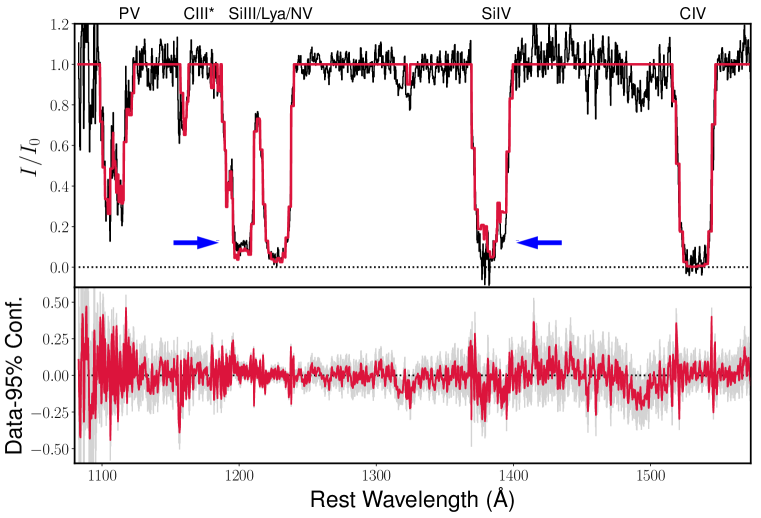
Figure 13: The results from an 11-bin tophat accordion model, using ionic columns from Cloudy runs using a hard spectral energy distribution (Korista et al., 1997). In the top panel, the median synthetic spectrum (crimson) is overlaid on the continuum-normalized spectrum (black). The lower panel shows the spectrum minus the median model and errors in gray, and the filled region between the spectrum and plus and minus the 95% confidence synthetic spectra in crimson, respectively. Overall, the fit is good, although the residuals show that the hard SED over-predicts the Ly$\alpha$ line, and under-predicts the Si IV line (marked by blue arrows).

The reduced $\chi^{2}$ for the hard SED model is 1.51 (1.26), compared with a value of 1.10 (1.16) for the soft SED and first (second) continuum models. As noted above, a value larger than 1.2 is excluded at 99% confidence level, suggesting that the synthetic spectrum produced using a soft SED provide a significantly better fit than that produced using a hard SED. Examination of the fit residuals shows that the model slightly over-predicts the Ly$\alpha$ line, and under-predicts the Si IV line, and those are the origins of the larger reduced $\chi^{2}$.

4.2.3 Effect of Metallicity

Some evidence exists for enhanced metallicity in quasars (e.g., Hamann & Ferland, 1999; Hamann et al., 2002; Kuraszkiewicz & Green, 2002). To address potential model dependence on metallicity, we performed a set of Cloudy runs using enhanced metallicity equivalent to $Z=3Z_{\odot}$. Following Hamann et al. (2002), all metals were set to three times their solar value, while nitrogen was set to nine times the solar value, and helium was set to 1.14 times the solar value. The relatively soft SED from Hamann et al. (2011) was used.

The results for the 11-bin tophat accordion model for the second continuum model are shown in Fig. 14. The result is similar for the first continuum model. As shown in Fig. 5, the reduced $\chi^{2}$ is consistently lower than for solar metallicity. The fit is somewhat better in the vicinity of Ly$\alpha$ and Si IV, as the model produced less neutral hydrogen and more Si⁺³ compared with the solar abundance model. In addition, the model includes the small C II lines near 1320Å.

We ran the enhanced metallicity models with 7, 8, 9, 10, 11, and 12 bins for both continua. The parameters as a function of velocity are shown in Fig. 7 and Fig. 8. The behavior as a function of velocity is similar to the solar metallicity case, although naturally $\log N_{H}-\log U$ is systematically lower. The largest, although still subtle, difference is an increase in column density and stronger decrease in ionization parameter around $v=-2400\rm\,km\,s^{-1}$.

As before, the column density seems to be roughly constant for velocities more negative than $-3300\rm\,km\,s^{-1}$, with an average column over that region of $\log N_{H}=21.6$ for the metals $\times 3$ case. The column density decreases at lower velocities, to an approximate constant level for velocities less negative than $-2800\rm\,km\,s^{-1}$ of $\log N_{H}=20.8\,\rm[cm^{-2}]$.

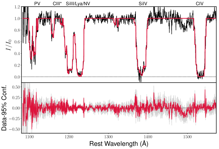
Figure 14: The results from an 11-bin tophat accordion model, using ionic columns from Cloudy runs using enhanced metallicity corresponding to $Z=3Z_{\odot}$. In the top panel, the median synthetic spectrum (crimson) is overlaid on the continuum-normalized spectrum (black). The lower panel shows the spectrum minus the median model and errors in gray, and the filled region between the spectrum and plus and minus the 95% confidence synthetic spectra in crimson, respectively. Overall, the higher metallicity model produces the best fit as it is able to fit the Si IV line well without predicting too much Ly$\alpha$.

4.3 Derived Quantities

Using the results of the MCMC, we computed derived quantities such as the total column density in the outflow, the radius of the outflow (as inferred from the concentration represented by C III*), the mass outflow rate, the momentum flux, and the kinetic luminosity of the outflow. In each case, we computed these parameters individually for each point in the MCMC chain (after cutting off the burnin), and then extracted the median points and $1\sigma$ error bars from the remainder.

We considered first the total hydrogen column density in the outflow. The results are shown in Fig. 15 as a function of the number of bins, spectral energy distribution, and metallicity. No strong dependence on the number of bins is seen, although a larger number of bins tends to yield a larger column density, as the model fits smaller-scale bumps and wiggles in the spectrum and the wings of the lines.

We obtained representative quantities of the derived parameters by taking the average over the 9–12 bin cases; the 7 and 8 bin cases, and the hard SED cases are not considered due to their less-than-acceptable fits (§4.1, Fig. 5).

The average total column density for the nominal, rather soft SED is $\log N_{H}=22.85$ (22.91) $\rm[cm^{-2}]$ for the first (second) continuum model. The hard SED (for an 11-bin model) yields much larger column density estimate, $\log N_{H}=23.4$ (23.3) $\rm[cm^{-2}]$. A harder continuum produces a larger Strömgren sphere (e.g., Casebeer et al., 2006, Fig. 13), so a larger column is needed to build up the columns of the relatively lower ionization lines such as Si IV and P V. The average column density for the enhanced metallicity case is $\log N_{H}=22.41$ (22.32) $\rm[cm^{-2}]$, about a factor of 2.2 times smaller than for the solar metallicity. This result makes sense, as more metal ions, responsible for most of the absorption lines, are available at the higher metallicity. The metallicity was enhanced by a factor of 3, and it is not immediately clear why the column density is not three times smaller than for the solar metallicity case, although as we noted above, the best fits for this model show a second peak in $\log N_{H}-\log U$ near $-2400\rm\,km\,s^{-1}$. It could be that the additional metals enhance the cooling in the photoionized gas, allowing the lower-ionization lines that constrain the column density to be present in a smaller column of gas.

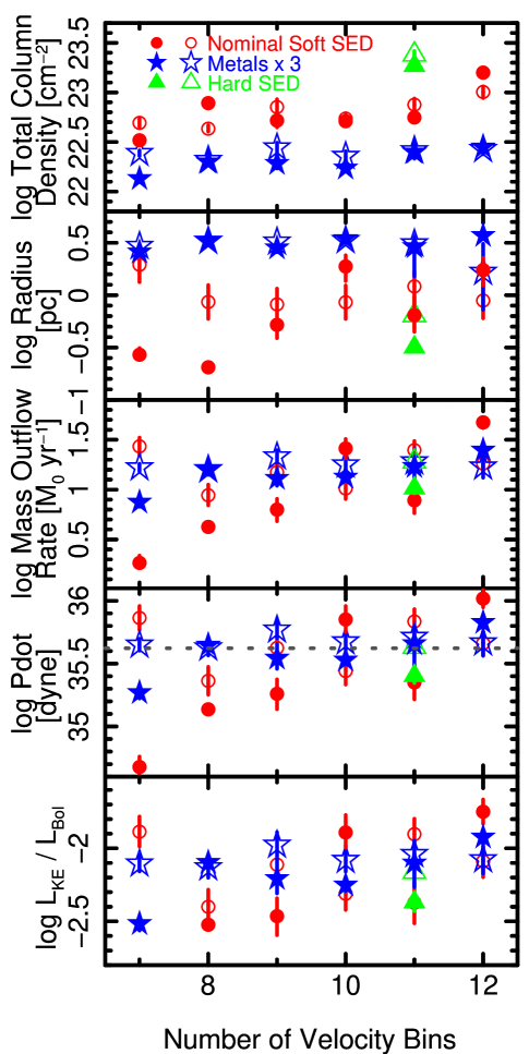
Figure 15: The derived quantities from the 26 models. In each case, the open (filled) symbols show the results using the first (second) continuum model. The top panel shows the total hydrogen column density in the outflow, weighted by the covering fraction in each bin. The second-from-the-top panel shows the radius of the outflow obtained using the density constraints in the concentration. The next panel shows the mass outflow rate, assuming that the radius of all outflow components is the same as the radius of the concentration. The fourth panel shows the momentum flux, $\dot{P}$, applying the same radius assumption, while the dashed line shows $L_{Bol}/c$. Finally, the bottom panel shows the ratio of the kinetic luminosity to the bolometric luminosity, again with the same radius assumption. See text for further details. In each case, the median and 1 sigma error bars obtained from the MCMC model are plotted.

The radius is related to the other parameters via

$$U=\frac{\phi}{nc}=\frac{Q}{4\pi R^{2}nc},$$

where $\phi$ is the photoionizing flux with units of $\rm photons\,s^{-1}\,cm^{-2}$, and $Q$ is the number of photoionizing photons per second emitted from the object. The density is constrained only within the concentration, so we compute the radius for those velocity bins only. We estimate $Q$ by scaling the Cloudy input spectral energy distribution to the observed spectrum (corrected for redshift and Milky Way reddening), and then integrating for energies greater than 13.6eV. The estimate of $\log Q=56.0$ is obtained assuming that there is no intrinsic reddening. Depending on the model, two to four bins represent the concentration. The radius for each simulation is taken to be the mean radius among those several values. The results are shown in Fig. 15.

The average inferred radius for the soft SED, solar metallicity, and first continuum model is $\log R=-0.027\,\rm pc$ (0.11 for the second continuum model), corresponding to 0.94 (1.3) pc. The average inferred radius for the higher metallicity case is $\log R=0.51\,\rm[pc]$ (0.53), or 3.2 (3.4) pc. The difference between radius estimates for the solar and $Z=3Z_{\odot}$ models originates in a small difference in preferred density in the concentration, being slightly higher for the solar metallicity (average $\log n=7.5$) than for the higher metallicity case (average $\log n=6.2$). The reason for this difference is not known; we speculate that it again has something to do with the cooling of the gas. At any rate, we can constrain the radius of the concentration to be 1–3 parsecs.

The radius is unconstrained at high and low velocities, because these regions, outside the concentration, are not represented in any density-sensitive lines in the observed bandpass. Thus the density outside of the concentration is unbounded in the spectral modeling. Since the density for velocity bins higher and lower than the concentration is unconstrained, it is consistent with the density of the concentration. We therefore assumed that the whole outflow is roughly co-spatial, and therefore assume that the inferred radius at high and low velocities is the same as the radius for the concentration.

Once we made this assumption, we can compute the mass outflow rate, given by Eq. 9 in Dunn et al. (2010) (see also Faucher-Giguère et al., 2012):

$$\dot{M}=8\pi\mu m_{p}\Omega RN_{H}v,$$

where the mean molecular weight $\mu=1.4$, the global covering fraction $\Omega$ is assumed to be 0.2, and we use the covering-fraction-weighted $N_{H}$ discussed above. $\dot{M}$ is computed for each bin using the velocity at the midpoint of each bin, and then summed over the whole profile. The results are shown in Fig. 15. The average $\log\dot{M}=1.23\,\rm[M_{\odot}\,yr^{-1}$] (1.44), or about 17 (28) solar masses per year for the first (second) continuum models. For the enhanced metallicity, the result was $\log\dot{M}=1.28\,\rm[M_{\odot}\,yr^{-1}$] (1.22), about 18.9 (16.5) solar masses per year. There is little difference between the solar metallicity and $Z=3Z_{\odot}$ results, despite the fact that the column density is lower for the $Z=3Z_{\odot}$ models. Apparently, the slightly higher values of radius for the $Z=3Z_{\odot}$ models combined with the slightly values of the lower column density to produce similar outflow rate estimates.

Next we computed the momentum flux $\dot{P}=\dot{M}v$ (e.g., Faucher-Giguère et al., 2012), shown in the fourth panel of Fig. 15. If the wind has an optical depth to photon scattering of $\tau\sim 1$, then the momentum flux would be on the order of the photon momentum $L_{bol}/c$. In addition, the momentum flux can be used to distinguish between momentum-conserving and energy-conserving outflows (e.g., Fiore et al., 2017). We also plotted an estimate of $\log L_{Bol}/c$. Luo et al. (2013) estimated a log bolometric luminosity of 46.1, based on scaling the Richards et al. (2006) template with the observed photometry and adding a contribution based on an estimate of the unabsorbed X-ray emission. We note that essentially the same value ($46.2$) was obtained from scaling the Cloudy SED to the observed continuum and integrating over it. Using the Luo et al. (2013) value, we obtain $\log L_{Bol}/c=35.6\,\rm[dynes]$. The average values are $\log\dot{P}=35.6\,\rm[dynes]$ (35.8) for solar metallicity, and $\log\dot{P}=35.7\,\rm[dynes]$ (35.7) for $Z=3Z_{\odot}$ for the first (second) continuum models, respectively. We found that the observed value of the momentum flux is very similar to the theoretical limit for a single photon scattering, suggesting that the outflow could be photon-momentum driven.

Finally, we computed the mechanical efficiency, the ratio of the kinetic luminosity to bolometric luminosity. The kinetic luminosity is given by Dunn et al. (Eq. 11 in 2010) as $\dot{E}_{k}=\dot{M}v^{2}/2$. The results are shown in Fig. 15. The mean value is $\log L_{KE}/L_{Bol}=-2.1$ ($-2.0$, excluding the 7- and 8-bin models), corresponding to about 0.8% (0.9%) for the solar metallicity case, and $\log L_{KE}/L_{Bol}=-2.04$ ($-2.09$), corresponding to 0.9% (0.8%) for the enhanced metallicity case, for the first (second) continuum models, respectively. These values fall within the range of the values required by simulations for effective feedback, 0.5% to 5% (Di Matteo et al., 2005; Hopkins & Elvis, 2010), albeit on the low end.

5 Discussion

5.1 The Black Hole Mass

As discussed above, we found that the outflow lies 1–3 pc from the central engine. In order to put this value into context, we estimated size scales in SDSS J0850$+$4451, beginning with the black hole mass.

To determine the radius of the broad line region, we referred to Bentz et al. (2013), who found that $\log(R_{BLR})=K+\alpha\log[\lambda L_{\lambda}(5100)/10^{44}\rm\,erg\,s^{-1}]$. The continuum flux density at 5100Å was estimated from the SDSS spectrum to be $F_{5100}=31.3\times 10^{-17}\rm\,erg\,s^{-1}\,cm^{-2}$Å^-1. Using the cosmological parameters used by Bentz et al. (2013) ($H_{0}=72\rm\,km/s/Mpc$, $\Omega_{M}=0.27$, and $\Omega_{\Lambda}=0.73$), we obtained a luminosity distance $D_{L}=3031\,\rm Mpc$. Using their best-fitting values $K=1.527^{+0.031}_{-0.031}$ and $\alpha=0.533^{+0.035}_{-0.033}$, we obtained an estimate of the radius of the broad-line region of 155 light days, corresponding to $0.13^{+0.024}_{-0.021}\rm\,pc$, where the uncertainties are based on the regression coefficient uncertainties.

SDSS J0850+4451 has been identified as having a disk-like H$\beta$ emission-line profile (Luo et al., 2013). Luo et al. (2013) fit the H$\beta$ line with a relativistic Keplerian disk model. They found inner and outer radii for the line of 450 and 4700 $r_{g}$ respectively. For our derived black hole mass, these values correspond to $r_{in}=0.035\rm\,pc$ and $r_{out}=0.37\rm\,pc$ respectively, roughly consistent with the Bentz et al. (2013) regression-estimated H$\beta$ radius of 0.13 pc.

We estimated the black hole mass from the H$\beta$ line in the SDSS spectrum in the usual way. The data and model are shown in Fig. 16. We were able to obtain a good fit with a single Gaussian profile with velocity width of $8090\pm 120\rm\,km\,s^{-1}$. To estimate the virial mass, we referred to Collin et al. (2006), who provide line-shape-based correction factors to the FWHM-based virial product used to estimate the black hole mass. For a Gaussian profile, $FWHM/\sigma_{line}=2.35$, and the scale factor for the mean spectrum is $f=0.835$. We estimated that the black hole mass is $1.6\times 10^{9}\rm\,M_{\odot}$. With the log bolometric luminosity estimate of 46.1, SDSS J0850+4451 is radiating at about 6% of the Eddington limit.

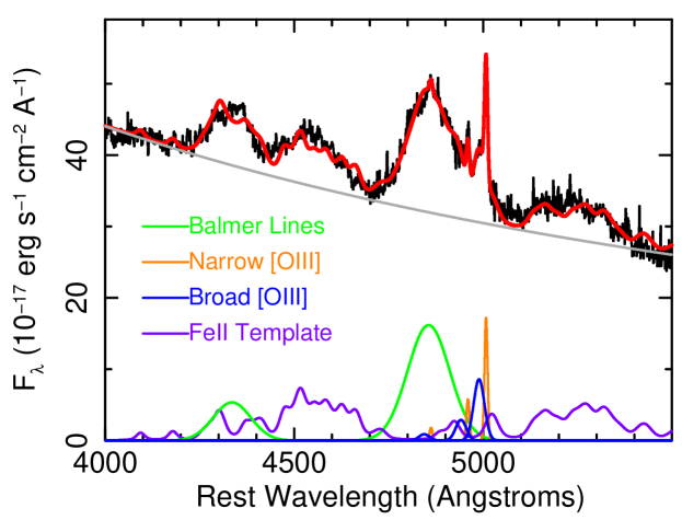
Figure 16: A model of the SDSS spectrum in the region of the H$\beta$ line. The broad H$\beta$ line was modeled with a single Gaussian, yielding a FWHM of $8090\pm 120\rm\,km\,s^{-1}$ and a black hole mass estimate of $1.6\times 10^{9}\rm\,M_{\odot}$. The small narrow H$\beta$ is the contribution from the narrow-line region, estimated to be 10% of the flux of [O III]$\lambda 5007$ (Cohen, 1983).

5.2 The Location of the Outflow

The analysis presented in §4.3 indicated that the outflow is located approximately 1–3 parsecs from the central engine, i.e., around the expected size of the torus in a quasar-luminosity object. Near-IR reverberation has shown that the location of the hot inner edge of the torus is correlated with the luminosity (Kishimoto et al., 2007). We used their Eq. 3 to estimate that the inner edge of the torus is $R_{\tau_{K}}=0.46\rm\,pc$, i.e., slightly smaller than the outflow distance.

Another number characterizing the torus is the $12\,\mu\rm m$ half-light radius. This property does not have a clear luminosity scaling relationship like $R_{\tau_{K}}$ (Burtscher et al., 2013). We estimated a plausible limit for $R_{1/2}(12\,\mu\rm m)$ by comparing the SDSS J0850$+$4451 bolometric luminosity with the objects in Burtscher et al. (2013) Table 6. Three objects have bolometric luminosities within 0.2 dex of SDSS J0850+4451, and all of these have upper limits on their mid-IR half-light radius between 2.7 and 3.5 parsecs. These estimates are crude, but they indicate that the outflow is consistent with an origin near the torus in SDSS J0850$+$4451. Interestingly, a torus location for the broad absorption line outflow in the Seyfert luminosity BALQ WPVS 007 was inferred based on variability arguments (Leighly et al., 2015).

Since we have estimated the black hole mass ($1.6\times 10^{9}\rm\,M_{\odot}$) and the radius of the outflow (1–3 parsecs), we can estimate the escape velocity $v_{esc}=\sqrt{2GM_{BH}/R}$ at the location of the outflow. We find that $v_{esc}$ lies between 2100 and $3700\,\rm km\,s^{-1}$, interestingly close to the range of velocities seen in the outflow. This result suggests that the outflow could have been accelerated from rest close to the location where it is observed, in contrast to large-distance outflows, where the outflow velocity is much greater than the escape velocity, and other acceleration mechanisms such as “cloud crushing” (e.g., Faucher-Giguère et al., 2012) are required.

5.3 The Acceleration Mechanism

We explored the acceleration mechanism for the outflow by using Cloudy to compute the force multiplier as a function of velocity. We extracted the MAP values of the ionization parameter and column density in each velocity bin, and assumed that the density over the whole outflow was equal to the average MAP value in bins representing the concentration. The results are shown in Fig. 17. As discussed in e.g., Couto et al. (2016), the force multiplier extracted from Cloudy is defined as the ratio of the total absorption cross section, including both line (bound-bound) and continuum (bound-free) processes, to the Thompson cross-section. The absorber can be radiatively driven if $FM\geq(L_{Bol}/L_{Edd})^{-1}$. As discussed in §5.1, this quasar seems to be radiating at about 6% of $L_{edd}$, which means that $\log FM$ should be greater than 1.2 for the outflow to be radiatively driven. Fig. 17 shows that for the solar metallicity case, the force multiplier is generally less than the required value, although it meets the required value for velocities between $-2600$ and $-1900\rm\,km\,s^{-1}$, implying that another source of acceleration (e.g., perhaps an MHD model, Kraemer et al., 2018) is necessary. On the other hand, for the $Z=3Z_{\odot}$ case, the force multiplier exceeds the required value significantly for velocities less than $\sim-2600\rm\,km\,s^{-1}$, suggesting that radiative driving may be important, at least at lower velocities in the outflow.

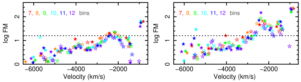
Figure 17: The force multiplier computed at the MAP solution as a function of velocity. The open symbols show the results for the first continuum model, and the solid symbols mark the solutions for the second continuum model. The left (right) panel shows the result for solar ($Z=3Z_{\odot}$) metallicity. The horizontal line marks the force multiplier value above which the flow can be radiatively driven. See the text for details.

The force multiplier is anti-correlated with the column density, and the ionization parameter (see Fig. 7 and Fig. 8). At larger velocities the gas may be thick but it may be too ionized to provide sufficient opacity for radiative driving. Alternatively, the gas may be too thick at high velocities (especially in the region of the concentration); a very thick gas slab is difficult to accelerate due to the loss of continuum photons by absorption (e.g., Arav & Li, 1994). This is shown by Baskin et al. (2014a) in their Fig. 9.

What is the origin of the differences between the solar metallicity case and the $Z=3Z_{\odot}$? We expect a larger force multiplier for a higher metallicity, as metals provide the bulk of the scattering opacity, as observed. The simulations also show that that a larger fraction of the acceleration in the higher metallicity case is attributed to bound-bound interactions. However, the offset between the $\log FM$ values is not constant between the two metallicity cases, suggesting a contribution from differences in the ionization state of the gas and column density as well.

The outflow in SDSS J0850$+$4451 originates near the torus. This suggests that dust could play a role in the wind acceleration. The equivalent dust cross section to scattering is 500–1000 times the electron scattering cross section for a typical quasar SED, which means that a typical quasar is super-Eddington with respect to dust, and may imply that dust-driven outflows can contribute to feedback (e.g., Fabian, 2012; Roth et al., 2012, and references therein). Some models for the torus that take into account radiation-driven outflows find that a strong wind is produced (e.g., Konigl & Kartje, 1994; Gallagher et al., 2015). For example, Chan & Krolik (2016) predict a wind along the inner edge of the torus with velocity $\sim 5000(M/10^{7}M_{\odot})^{1/4}[L_{UV}/(0.1L_{Edd})]^{1/4}\rm\,km\,s^{-1}$ that carries $\sim 0.1(M/10^{7}M_{\odot})^{3/4}[L_{UV}/(0.1L_{Edd}]^{3/4}\rm M_{\odot}\,yr^{-1}$ where $M$, $L_{UV}$, and $L_{Edd}$ are the black hole mass, UV luminosity, and Eddington luminosity respectively. Recent models of the broad line region also appeal to radiation pressure on dust (Czerny & Hryniewicz, 2011; Czerny et al., 2017; Baskin & Laor, 2018). Thus, it seems that radiative acceleration on dust may provide more than enough energy to power winds that originate in the vicinity of the torus and perhaps beyond.

The difficulty with this scenario is that while BALQ spectra are typically more reddened than quasars without broad absorption lines, only a small fraction show large amounts of reddening (e.g., 13% show $E(B-V)>0.1$ and 1.3% show $E(B-V)>0.2$, Krawczyk et al., 2015). SDSS J0850$+$4451, being UV selected, shows no evidence for reddening. In contrast, for a standard dust-to-gas ratio (Bohlin et al., 1978), a log hydrogen equivalent column density of 22.9 predicts $E(B-V)=13.7$, far too large to be realistic. So the dust must be separated from the gas. Dust is bound to the gas by collisions (Wickramasinghe et al., 1966), and that mechanism becomes inefficient at low densities, allowing the dust to drift. Evidence for this mechanism is found in AGB stars (Höfner & Olofsson, 2018, and references therein). We speculate that it is conceivable that the dusty wind is accelerated from the vicinity of the torus, and when it reaches a certain density, the dust continues to be accelerated, perhaps ultimately forming a scattering halo that may be observed as a polar outflow (Hönig et al., 2013; Hönig & Kishimoto, 2017), or be responsible for polarization in BALQs (Ogle et al., 1999) and red quasars (Alexandroff et al., 2018). The gas, which is left behind, would still have the momentum imparted during the dust acceleration phase, and could then be responsible for the broad absorption lines.

5.4 Where Does SDSS J0850$+$4451 Fit In?

In this paper, we have performed a detailed analysis of the absorption lines in SDSS J0850$+$4451. In this section, we compare SDSS J0850$+$4451 with other BALQs in order to gauge how typical this quasar is.

SDSS J0850$+$4451 was selected for observation using HST COS from a small sample of SDSS LoBAL quasars for which we had observations of He I*$\lambda 10830$ using either Gemini GNIRS and/or LBT LUCI. Our intention was to compare the optical depths of He I*$\lambda 10830$ and P V to investigate the nature of partial covering; this is discussed in Paper II (Leighly et al. in prep.). We used GALEX to ensure that the target objects would be bright enough for HST to obtain a good signal-to-noise ratio in a reasonable exposure time. Thus, SDSS J0850$+$4451 is relatively blue. SED fitting, to be presented in Paper II (Leighly et al.  in prep.) reveals no evidence for significant intrinsic reddening. In contrast, BALQs tend to be reddened compared with the normal quasar population, although many BALQs with little reddening are found (e.g., Krawczyk et al., 2015). Indeed, SED fitting of the optical and IR photometry shows that the torus emission is relatively weak (Paper II, Leighly et al. in prep.) suggesting that SDSS J0850$+$4451 might be relatively dust-free altogether.

Despite the lack of reddening, SDSS J0850$+$4451 was found to be X-ray weak in a Chandra observation (Luo et al., 2013). Only three hard photons, all with energies greater than 6.2 keV in the rest frame were detected. Assuming a typical quasar X-ray spectrum, Luo et al. (2013) found that a column of $N_{H}\approx 7\times 10^{23}\rm\,cm^{-2}$ was necessary to produce three hard photons and no soft photons. BALQs are known to be X-ray weak, and LoBAL quasars are known to be generally significantly X-ray weaker than high-ionization BALQs (e.g., Green et al., 2001; Gallagher et al., 2002a, 2006). Generally, this X-ray weakness is inferred to be due to absorption. Sometimes the column densities can be measured directly from the X-ray spectrum (e.g., Gallagher et al., 2002b), but often, only a few photons are detected, and the attenuation in the X-ray band compared with the optical band is assumed to originate from absorption, and in that case, the column density can be estimated. Luo et al. (2014) (their Fig. 4) shows that the $N_{H}$ estimated for SDSS J0850$+$4451 is relatively large compared with other BALQs. Alternatively, some BALQs have been shown to be intrinsically X-ray weak (e.g., Luo et al., 2014). That may not be the case for SDSS J0850$+$4451 as it shows relatively typical UV emission lines and ratios, in comparison with the weak line emission in the intrinsically X-ray weak quasar PHL 1811 (Leighly et al., 2007b, a). Nevertheless, it appears that SDSS J0850$+$4451 is typical LoBAL in its X-ray properties.

The broad absorption lines in SDSS J0850$+$4451 have a maximum velocity of $\sim-5500\rm\,km\,s^{-1}$ and a minimum velocity of $\sim-1400\rm\,km\,s^{-1}$, and therefore a width of about $4000\rm\,km\,s^{-1}$, and a middle velocity offset of $\sim-3500\rm\,km\,s^{-1}$. This velocity width appears to be rather typical of BALQs (Baskin et al., 2015). Several investigators have observed a rough upper envelope of maximum velocity with optical luminosity (Laor & Brandt, 2002; Ganguly et al., 2007). For $H_{0}=70\rm\,km\,s^{-1}\,Mpc^{-1}$, $\Omega_{M}=0.3$, $\Omega_{\Lambda}=0.7$, $\log\lambda L_{\lambda}$ at 3000Å is 45.4 [$\rm erg\,s^{-1}$]. Fig. 7 in Ganguly et al. (2007) shows that a maximum outflow velocity of $5500\rm\,km\,s^{-1}$ appears to be consistent with the average for an object with this luminosity.

As discussed in §5.1, the rather broad Balmer line observed in SDSS J0850$+$4451 yields a large black hole estimate of $1.6\times 10^{9}\rm\,M_{\odot}$, and for a bolometric luminosity estimate of $46.1\,\rm[erg\,s^{-1}]$ (Luo et al., 2013), the object is radiating at only 6% of Eddington. This value is low for a type 1 object. In contrast, Yuan & Wills (2003) observed $z\sim 2$ BALQs in the infrared band and found high (of order $\sim 1$) Eddington ratios. They noted that this might be a selection effect due to observing the brightest objects; on the other hand, they found that most objects had strong “Eigenvector 1” line emission patterns including very strong Fe II and weak [O III], also an indication of a high Eddington ratio. In contrast, SDSS J0850$+$4451, with its broad Balmer lines and modest Fe II emission has emission line properties mostly consistent with a low (for a Seyfert 1) accretion rate. The [O III] appears too weak for an object with such a broad H$\beta$ line, but weak [O III] seems to be common among LoBAL quasars (e.g., Schulze et al., 2017, and references therein). Empirically, it has been suggested that BALQs are typically high Eddington objects (e.g., Boroson, 2002), and this has also been suggested on theoretical grounds (Zubovas & King, 2013). SDSS J0850$+$4451’s low Eddington ratio would seem to make it anomalous, because, as shown in Ganguly et al. (2007) (their Fig. 6), very few of the Trump et al. (2006) BALQs radiate at less than 10% Eddington. However, a more recent study by Schulze et al. (2017) revealed no difference in black hole mass and Eddington ratio between a sample of 22 LoBAL quasars and unabsorbed objects, and several of their $z\sim 0.6$ sample showed Eddington ratios less than 10%. Thus general claims that all LoBALQs are high Eddington-ratio objects do not seem justified, although high Eddington-ratio objects may be over-represented in this population.

SDSS J0850$+$4451 has a kinetic-to-bolometric luminosity ratio for the broad absorption lines of 0.8–0.9% (Fig. 15). We note that there is also a blueshifted component of the [O III] line, modeled as an additional Gaussian with velocity offset of $-1150\rm\,km\,s^{-1}$ (§ 5.1), although we have no information about the spatial extent of this emission. Fiore et al. (2017) attempt to bring together a compendium of outflow indicators. While their information is incomplete for BALQ measurements, their results are nevertheless useful for comparison. Our $\dot{E}_{kin}/L_{bol}$ ratio is comparable to other BALQs and ionized winds for objects of the same bolometric luminosity. Like the other BALQs, our $v_{max}$ lies between the relatively low-velocity ionized gas and molecular outflows, and the ultra-fast outflows (UFOs). Our momentum flux ratio $\dot{P}_{OF}/\dot{P}_{AGN}$ is approximately 1, and is typical of ionized winds and UFOs, and less than the molecular outflows.

The outflow in SDSS J0850$+$4451 is located 1-3 parsecs from the central engine, consistent with the estimated location of the torus. Interestingly, a similar location was inferred for the broad absorption line outflow in the Seyfert-luminosity Narrow-line Seyfert 1 Galaxy WPVS 007 based on variability arguments (Leighly et al., 2015). Density-constrained distances have been measured for a handful of objects, and these span a wide range, from the vicinity of the torus (parsec scale) to kiloparsec scale (e.g., Lucy et al., 2014; Dabbieri et al., 2018; Arav et al., 2018). In comparison with the kiloparsec-scale outflows, the outflow in SDSS J0850$+$4451 appears to be relatively compact.

The discussion and comparisons above indicate that SDSS J0850$+$4451 has an outflow characterized by typical offset velocity and velocity width. But compared with other BALQs, it radiates at a relatively low Eddington ratio, has relatively broad emission lines, and has relatively low reddening and weak torus emission that suggest a low dust content. The outflow is observed near the torus, rather than at kiloparsec distances as has been found in some other BALQs, and therefore seems relatively compact. Although a conclusive comparison will have to wait until we have analyzed more objects, we suggest that the feedback interaction between the quasar nucleus and the host galaxy is not currently ongoing, although it may have been in the past. Indeed, SED fitting gave only an upper limit on the star-formation rate (Lazarova et al., 2012). Nevertheless, the outflow SDSS J0850$+$4451 hosts is likely to be important to the operation of the central engine. The accretion rate is estimated to be only $2.2\rm\,M_{\odot}\,yr^{-1}$, while the outflow rate is about 8 times higher. So if this object did not host an outflow, it might accrete at a higher rate, and the central engine and emission line properties might be much different.

6 Summary and Future Prospects

6.1 Summary of Results

In this paper, we present a detailed analysis of low redshift LoBAL quasar SDSS J0850$+$4451, using the novel spectral synthesis code SimBAL. Our principal results follow.

1. We introduced the SimBAL analysis method (§ 3). Using large grids of ionic column densities extracted from Cloudy models, we created synthetic spectra as a function of velocity, covering fraction, ionization parameter, density, and a combination column density parameter $\log N_{H}-\log U$. A forward-modeling spectral-synthesis approach was then used to compare the continuum-normalized HST spectrum with the synthetic spectra enabled by the Markov Chain Monte Carlo code emcee. The results included best-fitting spectra and posterior probability distributions of model parameters from which values and limits on physical parameters were extracted.

2. We investigated the systematics of our method by using two continuum models, two spectral energy distributions, a range of the number of velocity bins, and two values of the metallicity. Most of these combinations fit the data relatively well (Fig. 4, 6, 13), although the models with the smallest number of bins and the models using the hard spectral energy distribution are not favored statistically (Fig. 5).

3. Our models revealed interesting structure as a function of velocity (Fig. 7,8). The density-sensitive line C III* appears in the spectrum over a limited velocity range, and in this region, $\log N_{H}-\log U$ is larger than at other velocities. There is evidence that both $\log U$ and $\log N_{H}$ are larger at higher velocities. There is a strong decrease in covering fraction with velocity.

4. We were able to extract robust estimates of the total column density of the gas depending on the metallicity: 22.9 [$\rm cm^{-2}$] for solar, and 22.4 [$\rm cm^{-2}$] for $Z=3Z_{\odot}$. The density-sensitive line C III* line indicated a distance from the central engine of 1–3 parsecs. Assuming that all the gas lies at approximately the same distance from the central engine, we found that the mass outflow rate is 17–28 solar masses per year, the log of the momentum flux is 35.6–35.8 [dynes], consistent with $L_{Bol}/c$, and the ratio of the kinematic to bolometric luminosity is around 0.8–0.9%.

5. Using these results, we built a physical picture of the outflow in SDSS J0850$+$4451. The outflow location based on the gas density is consistent with an origin in the torus, where the escape velocity is interestingly close to the observed velocities in the outflow. Force multiplier analysis indicates that at least the lower velocity portions of the outflow might be consistent with acceleration by radiative line driving along our line of sight, and we speculated that dust scattering may also play a role, although selection for HST observation means that SDSS J0850$+$4451 is a relatively blue object lacking the reddening that is common in BALQs in general and LoBALQs specifically. SDSS J0850$+$4451 has an Eddington ratio of just 6%, lower than that of the general population of BALQs. Given the compact nature of the outflow, we speculated that SDSS J0850$+$4451 is past the era of feedback, if it occurred previously. A JWST study of its host galaxy to determine whether it is quiescent or star-forming would be an interesting follow-up. Nevertheless, we contend that the outflow is of integral importance to the nature of the central engine, since the outflow rate is estimated to be nearly an order of magnitude greater than the accretion rate.

6.2 The Future

SimBAL has enabled us to perform an analysis of the rest-frame UV broad absorption line outflow in the low-redshift quasar SDSS J0850$+$4451 that is unprecedented in detail. Clearly, however, the real power of SimBAL will be manifest when we compare SDSS J0850$+$4451 with other objects. For example, it will be interesting to compare with analysis of SDSS J142927.28$+$523849.5, a second object observed as part of our HST program, that shows strong Eigenvector-1 properties, i.e, a narrow H$\beta$ line and strong Fe II emission, likely indicating a high accretion rate (Leighly et al. 2018, in prep.). But that is only the beginning. Large samples from SDSS/BOSS can be analyzed to infer the general properties of outflows. It should be emphasized that these are physical properties of the gas, rather than the empirical properties (e.g., balnicity, maximum depth, width, maximum velocity) that dominate BALQ studies today. We will be able to, for example, determine ionization parameters, column densities, and covering fractions in a large number of objects. Densities and outflow radii will be extracted from a subset. For example, analysis of a sample of FeLoBALs has revealed outflow radii that span four orders of magnitude, and a general lack of broad lines at kpc scales (Dabbieri et al., 2018, Leighly et al. in prep.). We will be able to look for trends as a function of velocity among outflows; for example, perhaps the covering fractions usually decrease with increasing velocity. We will be able to learn whether outflow concentrations such as the one observed in SDSS J0850$+$4451 are common, or whether the gas properties are more uniform generally. We believe that SimBAL will be able to revolutionize the study of broad absorption line quasars.

To reach the full potential of the approach, several improvements are being implemented. An important one is that we need to account for systematic uncertainties due to continuum model and placement. We are developing a principal components analysis approach that will allow us to simultaneously model the absorption and the continuum (Marrs et al., 2017; Wagner et al., 2017), which has already been implemented in the near-UV (Leighly et al., 2017; Dabbieri et al., 2018, Leighly et al., in prep.). The far UV is a harder nut to crack, given the Ly$\alpha$ forest contamination, and we are currently testing some promising approaches (Choi et al. 2018, in prep.). Other improvements, either implemented or planned, include schemes to speed up the code, reduce the memory requirements, and implement various automated checks on the solutions, as well as an interactive interface that can be used to generate starting points. We plan to release the software to the community once it is fully vetted.

Appendix A Potential Systematic Effects

In this paper, we build upon current state-of-the-art methods for quantitative comparison of spectra with photoionization models. In these methods, the photoionization models are constructed assuming a constant density and dust-free slab of gas (e.g., Moe et al., 2009; Dunn et al., 2010; Arav et al., 2013; Borguet et al., 2012, 2013; Lucy et al., 2014; Chamberlain et al., 2015; Xu et al., 2018). It is possible that those assumptions can be tested with SimBAL. In this section, we perform some limited tests; a more comprehensive discussion is beyond the scope of this paper. We use as an example one of our solutions, an 11-bin model using the nominal soft spectral energy distribution and solar abundances fit to the spectrum normalized by the first continuum model.

A.1 Dust

The inferred location of the absorbing gas in SDSS J0850$+$4451 is 1–$3\rm\,pc$ (§ 4.3). This distance is larger than the dust sublimation radius, estimated to be about 0.2 pc based on the inferred bolometric luminosity (Laor & Draine, 1993). It therefore may be expected that dust would be present in the absorbing outflow. Dust dramatically alters the photoionized ionic column densities due to attenuation of the continuum and metal depletion. As discussed in §5.4, and discussed in more detail in Paper II (Leighly et al. in prep.), SDSS J0850$+$4451 was selected from among our He I* BALSQSOs because GALEX photometry showed that it bright enough in the UV to observe using HST in a reasonable amount of time. Thus, SDSS J0850$+$4451 is a rather blue object, and spectral energy distribution modeling of the broad band photometry indicates that reddening is negligible (Paper II; Leighly et al. in prep.). There is therefore no evidence for dust in the absorber in SDSS J0850$+$4451.

The recent literature indicates that dust seems to be quite complicated in quasars and AGN. In several objects, anomalously steep and unusually-shaped reddening curves have been found (e.g., Leighly et al., 2009; Jiang et al., 2013; Leighly et al., 2014). In Mrk 231, we found that the unusual reddening curve was similar to those previously used to explain the low values of total-to-selective extinction in Type Ia supernovae (Leighly et al., 2014). While SMC extinction generally provides a good fit to quasar photometry (Krawczyk et al., 2015), Zafar et al. (2015) find extinction curves for heavily reddened quasars that are steeper than the SMC, although their results may depend somewhat on the assumed shape of the intrinsic continuum (Collinson et al., 2017). They speculate that large dust grains might be destroyed by the active nucleus. Gallerani et al. (2010) found that the extinction laws for high redshift quasars deviate significantly from the SMC, being flatter in the UV. This trend was particularly pronounced for BALQs. They suggest that the difference between high and low redshift quasars may originate in the fact that the relative contribution of AGBs and SNes in quasars is strongly dependent on the star formation history and the age of the Universe.

Nonetheless, the question of the presence of dust in outflows is interesting. Leighly et al. (2014) explored dust and depletion in some detail in Mrk 231, a heavily reddened object in which the presence of dust is undeniable. We found that dust was necessary to produce the Na I absorption line without requiring an unreasonably large column density. We also found evidence for density enhancement in the partially ionized zone (from, e.g., a shock). While it was possible to perform a thorough exploration of parameter space for a single object, it is not feasible to include so many independent parameters in SimBAL. In the future, as appropriate, we may attempt to analyze the effect of dust, perhaps in a binary way, as we have explored the dependence on metallicity and spectral energy distribution in this paper.

A.2 Filtering

Our tophat opacity model splits the absorption profile into adjacent velocity bins, allowing us to derive physical parameters of the outflow as a function of velocity. This information may ultimately help us constrain the origin and acceleration of the outflows. Biased by the fact that we observe only the radial component of the outflow, it is tempting to interpret the tophat model physically, i.e., to assume that we are seeing an accelerating outflow, with the lowest velocity slab closest to the continuum source, and higher velocity slabs sequentially behind one another. If this were the case, then one would expect outer slabs to be illuminated by the transmitted continuum of inner slabs. Alternatively, the flow could be decelerating. The transmitted continuum would be deficient in photons of certain energies, depending on the ionization parameter and thickness of the bin. Filtering may play a role in producing the characteristic intermediate-ionization emission lines in Narrow-line Seyfert 1 galaxies (Leighly, 2004), and has been used to explain the lack of the He I$\lambda 5876$ emission line in weak-line quasar PHL 1811 (Leighly et al., 2007a). It is not clear whether filtering plays an important role in BAL outflows.

Starting with the 11-bin model illuminated by the soft spectral energy distribution and solar abundances, we tested both acceleration and deceleration scenarios, as follows. For acceleration, we first redshifted the illuminating continuum by the offset velocity of the lowest-velocity bin. We ran the Cloudy simulation, and extracted the total (i.e., including diffuse emission) transmitted continuum. To take the covering fraction into account, we computed the inferred opacity as a function of energy (the continua are represented in Rydbergs) and used the power-law partial covering model to compute the inferred $I/I_{0}$. Multiplying by the input continuum gave the covering-fraction weighted transmitted continuum. We redshifted this continuum to account for the velocity offset of the next bin, and illuminated the second bin, harvesting the transmitted continuum, and so on through the eleven bins. The resulting continua transmitted through the whole outflow for the accelerating and decelerating cases are shown in Fig. 18. Since the simulation is matter bounded, we do not lose much light in the hydrogen continuum; the ionization parameter $U$ (computed from 1 Rydberg to higher energies) decreases by only 50%. In contrast, the decrease in the helium continuum is dramatic; ionization parameter $U$ computed for $E>4\rm\,Rydbergs$ is lower by a factor of 150.

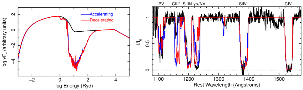
Figure 18: Tests of the effect of the effect of filtering. Left: The filtered continua for the accelerating (blue) and decelerating (red) cases, compared with the unabsorbed continuum (black), computed as described in the text. The filtered continua are not much different from the unabsorbed in the hydrogen continuum (0–4 Rydbergs), but are much weaker in the helium continuum ($>4\rm\,Rydbergs$). Right: The SDSS J0850$+$4451 spectrum overlaid with the best-fit 11-bin nominal SED solar abundance model subject to filtering, as described in the text. The signature of acceleration (blue) and deceleration (red) are strongly seen in N V absorption line, with the decrease in opacity at high and low velocities, respectively.

The resulting synthetic spectra are shown in Fig. 18. The C IV and Si IV are largely unaffected. This is expected since the hydrogen continuum is not much altered by filtering and the ionization potentials to create C⁺³ (47.9 eV) and Si⁺³ (33.5 eV) are both less than 4 Rydbergs (54.4 eV). In contrast, N V, with ionization potential to create N${}^{+4}=77.5\rm\,eV$, is strongly affected. The signature of acceleration and deceleration are clearly seen, from the decrease of N V opacity at high and low velocities, respectively.

The other large change in the synthetic spectrum is in the C III* line. As seen in Fig. 10, this line is sensitive to column density. For a fixed $\log N_{H}-\log U$, with the ionization parameter effectively decreasing as the continuum becomes more and more filtered, the slab produces more lower-ionization lines at the back end than before.

This result, although limited in generality, is very instructive nonetheless. If filtering is typically important in BAL outflows, we would expect to measure a consistent increase or decrease in ionization with velocity. Generally speaking, we do not see that. High-ionization lines are usually the broadest of all, encompassing low-ionization lines in velocity space. For example, O VI lines are often inferred to be very broad (e.g., Leighly et al., 2009). Instead, in the case of SDSS J0850$+$4451, we find that the ionization parameter varies only subtly with velocity (Fig. 6 and Fig. 7).

It therefore seems that gas at all velocities is illuminated by the continuum from the central engine. This may mean that the direction of the outflow is oblique to the line of sight (e.g., Arav, 2004, Fig. 3), so gas at all velocities have a clear view of the nucleus. It is also not clear what the role of partial covering is in the question of filtering. By definition, gas that partially covers the continuum leaves part of the line of sight free from obscuration so that the continuum can illuminate gas at larger radii free from attenuation.

A.3 Constant Pressure

Baskin et al. (2014b) suggested that radiation pressure compression (confinement) may apply to broad absorption line outflows, although they did not perform a quantitative comparison with spectra. Radiation pressure confinement was first applied to the narrow-line region in AGN by Dopita et al. (2002). This model has been subsequently applied to the extended narrow line region by Stern et al. (2014b), to the broad line region by Baskin et al. (2014a), and to warm absorbers by Stern et al. (2014a). This model assumes constant total pressure in the photoionized slab, rather than constant density.

We tested this scenario by running constant pressure models using the best-fit parameters for the 11-bin soft SED solar abundances model. We did not expect dramatic differences between the constant density and constant pressure models for SDSS J0850$+$4451 because the outflows are optically thin to the Hydrogen continuum, and are therefore matter bounded rather than ionization bounded. Our previous experience with constant pressure and compression in the context of Mrk 231 (Leighly et al., 2014) suggested that many of the differences between constant density and constant pressure occur near the hydrogen ionization front and in the partially ionized zone. As discussed Stern et al. (2016), in the context of emission line models, gas can be most effectively compressed if ionization bounded (rather than matter bounded, as in SDSS J0850$+$4451) so that there is a slab of mostly neutral material against which the ionized gas can be compressed.

The blue line in Fig. 19 shows this model overlaid on the data. The appearance of strong low-ionization lines such as C II$\lambda 1335$ that are not observed, and comparison with Fig. 10 (especially the accompanying animations) suggests that the column density is slightly too high. We tested this idea by performing an MCMC simulation, allowing the eleven values of $\log N_{H}-\log U$ to be free, and fixing the other parameters at their best-fitting values. The red line shows that the resulting simulated spectrum agrees very well with the observed spectrum. The reduced $\chi^{2}$ is 1.28, higher than the value for the best fitting constant density model of 1.11. Undoubtedly, a better fit could be obtained if all parameters were allowed to vary. That experiment is beyond the scope of this paper, and may be interesting to pursue in future work.

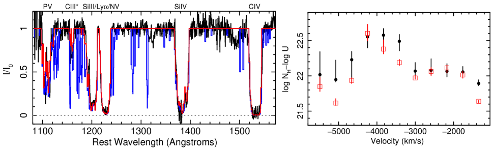
Figure 19: Tests of the effect of the constant pressure assumption. Left: The SDSS J0850$+$4451 spectrum overlaid with the best-fit 11-bin soft SED solar abundance model with the total pressure constrained to be constant (blue line). Comparison with Fig. 10 shows that the $\log N_{H}-\log U$ appears to be too high. The red line shows the same model with $\log N_{H}-\log U$ allowed to vary, yielding an acceptable fit. Right: The best fitting $\log N_{H}-\log U$ parameters for the best fit shown in Fig. 4 (black), and the best-fitting constant pressure values (red). The constant pressure model indicates a slightly lower column density.

The log of the covering fraction-weighted column density from the constant density best fit was $22.88\pm 0.06$ [$\rm cm^{-2}$] (95% uncertainties). For the constant pressure and variable $\log N_{H}-\log U$ model, the log of the covering fraction-weighted column density was $22.71^{+0.04}_{-0.03}$ [$\rm cm^{-2}$]. It is expected that the total column density should be slightly lower, as observed, since in a constant pressure model, the density increases into the slab and therefore the more highly ionized gas is found closer to the illuminated face. The difference in total hydrogen column density in this case is very small, as expected.

References

- Alexandroff et al. (2018) Alexandroff, R. M., Zakamska, N. L., Barth, A. J., et al. 2018, MNRAS
- Arav (2004) Arav, N. 2004, in Astronomical Society of the Pacific Conference Series, Vol. 311, AGN Physics with the Sloan Digital Sky Survey, ed. G. T. Richards & P. B. Hall, 213
- Arav et al. (2013) Arav, N., Borguet, B., Chamberlain, C., Edmonds, D., & Danforth, C. 2013, MNRAS, 436, 3286
- Arav et al. (2005) Arav, N., Kaastra, J., Kriss, G. A., et al. 2005, ApJ, 620, 665
- Arav & Li (1994) Arav, N., & Li, Z.-Y. 1994, ApJ, 427, 700
- Arav et al. (2018) Arav, N., Liu, G., Xu, X., et al. 2018, ApJ, 857, 60
- Arav et al. (2001) Arav, N., de Kool, M., Korista, K. T., et al. 2001, ApJ, 561, 118
- Baskin & Laor (2018) Baskin, A., & Laor, A. 2018, MNRAS, 474, 1970
- Baskin et al. (2015) Baskin, A., Laor, A., & Hamann, F. 2015, MNRAS, 449, 1593
- Baskin et al. (2014a) Baskin, A., Laor, A., & Stern, J. 2014a, MNRAS, 438, 604
- Baskin et al. (2014b) —. 2014b, MNRAS, 445, 3025
- Bautista et al. (2010) Bautista, M. A., Dunn, J. P., Arav, N., et al. 2010, ApJ, 713, 25
- Bentz et al. (2013) Bentz, M. C., Denney, K. D., Grier, C. J., et al. 2013, ApJ, 767, 149
- Bohlin et al. (1978) Bohlin, R. C., Savage, B. D., & Drake, J. F. 1978, ApJ, 224, 132
- Borguet et al. (2013) Borguet, B. C. J., Arav, N., Edmonds, D., Chamberlain, C., & Benn, C. 2013, ApJ, 762, 49
- Borguet et al. (2012) Borguet, B. C. J., Edmonds, D., Arav, N., Benn, C., & Chamberlain, C. 2012, ApJ, 758, 69
- Boroson (2002) Boroson, T. A. 2002, ApJ, 565, 78
- Branch et al. (2005) Branch, D., Baron, E., Hall, N., Melakayil, M., & Parrent, J. 2005, PASP, 117, 545
- Burtscher et al. (2013) Burtscher, L., Meisenheimer, K., Tristram, K. R. W., et al. 2013, A&A, 558, A149
- Casebeer et al. (2006) Casebeer, D. A., Leighly, K. M., & Baron, E. 2006, ApJ, 637, 157
- Chamberlain et al. (2015) Chamberlain, C., Arav, N., & Benn, C. 2015, MNRAS, 450, 1085
- Chan & Krolik (2016) Chan, C.-H., & Krolik, J. H. 2016, ApJ, 825, 67
- Cohen (1983) Cohen, R. D. 1983, ApJ, 273, 489
- Collin et al. (2006) Collin, S., Kawaguchi, T., Peterson, B. M., & Vestergaard, M. 2006, A&A, 456, 75
- Collinson et al. (2017) Collinson, J. S., Ward, M. J., Landt, H., et al. 2017, MNRAS, 465, 358
- Couto et al. (2016) Couto, J. D., Kraemer, S. B., Turner, T. J., & Crenshaw, D. M. 2016, ApJ, 833, 191
- Czerny & Hryniewicz (2011) Czerny, B., & Hryniewicz, K. 2011, A&A, 525, L8
- Czerny et al. (2017) Czerny, B., Li, Y.-R., Hryniewicz, K., et al. 2017, ApJ, 846, 154
- Dabbieri et al. (2018) Dabbieri, C., Choi, H., MacInnis, F., Leighly, K., & Terndrup, D. 2018, in American Astronomical Society Meeting Abstracts, Vol. 231, American Astronomical Society Meeting Abstracts #231, 250.14
- de Kool et al. (2001) de Kool, M., Arav, N., Becker, R. H., et al. 2001, ApJ, 548, 609
- de Kool et al. (2002a) de Kool, M., Becker, R. H., Arav, N., Gregg, M. D., & White, R. L. 2002a, ApJ, 570, 514
- de Kool et al. (2002b) de Kool, M., Becker, R. H., Gregg, M. D., White, R. L., & Arav, N. 2002b, ApJ, 567, 58
- de Kool et al. (2002c) de Kool, M., Korista, K. T., & Arav, N. 2002c, ApJ, 580, 54
- Di Matteo et al. (2005) Di Matteo, T., Springel, V., & Hernquist, L. 2005, Nature, 433, 604
- Dopita et al. (2002) Dopita, M. A., Groves, B. A., Sutherland, R. S., Binette, L., & Cecil, G. 2002, ApJ, 572, 753
- Dunn et al. (2010) Dunn, J. P., Bautista, M., Arav, N., et al. 2010, ApJ, 709, 611
- Fabian (2012) Fabian, A. C. 2012, ARA&A, 50, 455
- Faucher-Giguère et al. (2012) Faucher-Giguère, C.-A., Quataert, E., & Murray, N. 2012, MNRAS, 420, 1347
- Ferland et al. (2013) Ferland, G. J., Porter, R. L., van Hoof, P. A. M., et al. 2013, Rev. Mexicana Astron. Astrofis., 49, 137
- Ferrarese & Merritt (2000) Ferrarese, L., & Merritt, D. 2000, ApJ, 539, L9
- Finn et al. (2014) Finn, C. W., Morris, S. L., Crighton, N. H. M., et al. 2014, MNRAS, 440, 3317
- Fiore et al. (2017) Fiore, F., Feruglio, C., Shankar, F., et al. 2017, A&A, 601, A143
- Foreman-Mackey et al. (2013) Foreman-Mackey, D., Hogg, D. W., Lang, D., & Goodman, J. 2013, PASP, 125, 306
- Francis et al. (1991) Francis, P. J., Hewett, P. C., Foltz, C. B., et al. 1991, ApJ, 373, 465
- Gabel et al. (2005) Gabel, J. R., Kraemer, S. B., Crenshaw, D. M., et al. 2005, ApJ, 631, 741
- Gallagher et al. (2002a) Gallagher, S. C., Brandt, W. N., Chartas, G., & Garmire, G. P. 2002a, ApJ, 567, 37
- Gallagher et al. (2002b) Gallagher, S. C., Brandt, W. N., Chartas, G., Garmire, G. P., & Sambruna, R. M. 2002b, ApJ, 569, 655
- Gallagher et al. (2006) Gallagher, S. C., Brandt, W. N., Chartas, G., et al. 2006, ApJ, 644, 709
- Gallagher et al. (2015) Gallagher, S. C., Everett, J. E., Abado, M. M., & Keating, S. K. 2015, MNRAS, 451, 2991
- Gallerani et al. (2010) Gallerani, S., Maiolino, R., Juarez, Y., et al. 2010, A&A, 523, A85
- Ganguly et al. (2007) Ganguly, R., Brotherton, M. S., Cales, S., et al. 2007, ApJ, 665, 990
- Goodman & Weare (2010) Goodman, J., & Weare, J. 2010, Communications in Applied Mathematics and Computational Science, Vol. 5, No. 1, p. 65-80, 2010, 5, 65
- Green et al. (2001) Green, P. J., Aldcroft, T. L., Mathur, S., Wilkes, B. J., & Elvis, M. 2001, ApJ, 558, 109
- Hamann (1997) Hamann, F. 1997, ApJS, 109, 279
- Hamann (1998) —. 1998, ApJ, 500, 798
- Hamann et al. (2013) Hamann, F., Chartas, G., McGraw, S., et al. 2013, MNRAS, 435, 133
- Hamann & Ferland (1999) Hamann, F., & Ferland, G. 1999, ARA&A, 37, 487
- Hamann et al. (2011) Hamann, F., Kanekar, N., Prochaska, J. X., et al. 2011, MNRAS, 410, 1957
- Hamann & Korista (1996) Hamann, F., & Korista, K. T. 1996, ApJ, 464, 158
- Hamann et al. (2002) Hamann, F., Korista, K. T., Ferland, G. J., Warner, C., & Baldwin, J. 2002, ApJ, 564, 592
- Hamann et al. (2001) Hamann, F. W., Barlow, T. A., Chaffee, F. C., Foltz, C. B., & Weymann, R. J. 2001, ApJ, 550, 142
- Hauschildt & Baron (1999) Hauschildt, P. H., & Baron, E. 1999, Journal of Computational and Applied Mathematics, 109, 41
- Hewett & Wild (2010) Hewett, P. C., & Wild, V. 2010, MNRAS, 405, 2302
- Höfner & Olofsson (2018) Höfner, S., & Olofsson, H. 2018, A&A Rev., 26, 1
- Hönig & Kishimoto (2017) Hönig, S. F., & Kishimoto, M. 2017, ApJ, 838, L20
- Hönig et al. (2013) Hönig, S. F., Kishimoto, M., Tristram, K. R. W., et al. 2013, ApJ, 771, 87
- Hopkins & Elvis (2010) Hopkins, P. F., & Elvis, M. 2010, MNRAS, 401, 7
- Jiang et al. (2013) Jiang, P., Zhou, H., Ji, T., et al. 2013, AJ, 145, 157
- King & Pounds (2015) King, A., & Pounds, K. 2015, ARA&A, 53, 115
- Kishimoto et al. (2007) Kishimoto, M., Hönig, S. F., Beckert, T., & Weigelt, G. 2007, A&A, 476, 713
- Konigl & Kartje (1994) Konigl, A., & Kartje, J. F. 1994, ApJ, 434, 446
- Korista et al. (1997) Korista, K., Baldwin, J., Ferland, G., & Verner, D. 1997, ApJS, 108, 401
- Kormendy & Ho (2013) Kormendy, J., & Ho, L. C. 2013, ARA&A, 51, 511
- Kraemer et al. (2018) Kraemer, S. B., Tombesi, F., & Bottorff, M. C. 2018, ApJ, 852, 35
- Krawczyk et al. (2015) Krawczyk, C. M., Richards, G. T., Gallagher, S. C., et al. 2015, AJ, 149, 203
- Kuraszkiewicz & Green (2002) Kuraszkiewicz, J. K., & Green, P. J. 2002, ApJ, 581, L77
- Laor & Brandt (2002) Laor, A., & Brandt, W. N. 2002, ApJ, 569, 641
- Laor & Draine (1993) Laor, A., & Draine, B. T. 1993, ApJ, 402, 441
- Lazarova et al. (2012) Lazarova, M. S., Canalizo, G., Lacy, M., & Sajina, A. 2012, ApJ, 755, 29
- Leighly et al. (2017) Leighly, K., Marrs, A., Wagner, C., & Macinnis, F. 2017, in American Astronomical Society Meeting Abstracts, Vol. 229, American Astronomical Society Meeting Abstracts, 250.16
- Leighly (2004) Leighly, K. M. 2004, ApJ, 611, 125
- Leighly et al. (2015) Leighly, K. M., Cooper, E., Grupe, D., Terndrup, D. M., & Komossa, S. 2015, ApJ, 809, L13
- Leighly et al. (2011) Leighly, K. M., Dietrich, M., & Barber, S. 2011, ApJ, 728, 94
- Leighly et al. (2007a) Leighly, K. M., Halpern, J. P., Jenkins, E. B., & Casebeer, D. 2007a, ApJS, 173, 1
- Leighly et al. (2007b) Leighly, K. M., Halpern, J. P., Jenkins, E. B., et al. 2007b, ApJ, 663, 103
- Leighly et al. (2009) Leighly, K. M., Hamann, F., Casebeer, D. A., & Grupe, D. 2009, ApJ, 701, 176
- Leighly et al. (2014) Leighly, K. M., Terndrup, D. M., Baron, E., et al. 2014, ApJ, 788, 123
- Lucy et al. (2014) Lucy, A. B., Leighly, K. M., Terndrup, D. M., Dietrich, M., & Gallagher, S. C. 2014, ApJ, 783, 58
- Luo et al. (2013) Luo, B., Brandt, W. N., Alexander, D. M., et al. 2013, ApJ, 772, 153
- Luo et al. (2014) —. 2014, ApJ, 794, 70
- Marrs et al. (2017) Marrs, A., Leighly, K., Wagner, C., & Macinnis, F. 2017, in American Astronomical Society Meeting Abstracts, Vol. 229, American Astronomical Society Meeting Abstracts #229, 250.14
- Moe et al. (2009) Moe, M., Arav, N., Bautista, M. A., & Korista, K. T. 2009, ApJ, 706, 525
- Moravec et al. (2017) Moravec, E. A., Hamann, F., Capellupo, D. M., et al. 2017, MNRAS, 468, 4539
- Ogle et al. (1999) Ogle, P. M., Cohen, M. H., Miller, J. S., et al. 1999, ApJS, 125, 1
- Osterman et al. (2011) Osterman, S., Green, J., Froning, C., et al. 2011, Ap&SS, 335, 257
- Pâris et al. (2011) Pâris, I., Petitjean, P., Rollinde, E., et al. 2011, A&A, 530, A50
- Richards et al. (2006) Richards, G. T., Lacy, M., Storrie-Lombardi, L. J., et al. 2006, ApJS, 166, 470
- Roth et al. (2012) Roth, N., Kasen, D., Hopkins, P. F., & Quataert, E. 2012, ApJ, 759, 36
- Rupke et al. (2002) Rupke, D. S., Veilleux, S., & Sanders, D. B. 2002, ApJ, 570, 588
- Sabra & Hamann (2001) Sabra, B. M., & Hamann, F. 2001, ApJ, 563, 555
- Savage & Sembach (1991) Savage, B. D., & Sembach, K. R. 1991, ApJ, 379, 245
- Schlafly & Finkbeiner (2011) Schlafly, E. F., & Finkbeiner, D. P. 2011, ApJ, 737, 103
- Schulze et al. (2017) Schulze, A., Schramm, M., Zuo, W., et al. 2017, ApJ, 848, 104
- Shen et al. (2011) Shen, Y., Richards, G. T., Strauss, M. A., et al. 2011, ApJS, 194, 45
- Stern et al. (2014a) Stern, J., Behar, E., Laor, A., Baskin, A., & Holczer, T. 2014a, MNRAS, 445, 3011
- Stern et al. (2016) Stern, J., Faucher-Giguère, C.-A., Zakamska, N. L., & Hennawi, J. F. 2016, ApJ, 819, 130
- Stern et al. (2014b) Stern, J., Laor, A., & Baskin, A. 2014b, MNRAS, 438, 901
- Trump et al. (2006) Trump, J. R., Hall, P. B., Reichard, T. A., et al. 2006, ApJS, 165, 1
- Wagner et al. (2017) Wagner, C., Leighly, K., Macinnis, F., Marrs, A., & Richards, G. T. 2017, in American Astronomical Society Meeting Abstracts, Vol. 229, American Astronomical Society Meeting Abstracts #229, 250.15
- Wang et al. (2010) Wang, H., Wang, T., Yuan, W., et al. 2010, ApJ, 710, 78
- Wickramasinghe et al. (1966) Wickramasinghe, N. C., Donn, B. D., & Stecher, T. P. 1966, ApJ, 146, 590
- Xu et al. (2018) Xu, X., Arav, N., Miller, T., & Benn, C. 2018, ArXiv e-prints
- Yuan & Wills (2003) Yuan, M. J., & Wills, B. J. 2003, ApJ, 593, L11
- Zafar et al. (2015) Zafar, T., Møller, P., Watson, D., et al. 2015, A&A, 584, A100
- Zubovas & King (2013) Zubovas, K., & King, A. 2013, ApJ, 769, 51