Muon $g-2$ in a $U(1)$-symmetric Two-Higgs-Doublet Model

Abstract

We show in this paper that, in a $U(1)$-symmetric two-Higgs-doublet model (2HDM), the two additional neutral Higgs bosons would become nearly degenerate in the large $\tan\beta$ regime, under the combined constraints from both theoretical arguments and experimental measurements. As a consequence, the excess observed in the anomalous magnetic moment of the muon could not be addressed in the considered framework, following the usual argument where these two neutral scalars are required to manifest a large mass hierarchy. On the other hand, we find that, with an $\mathcal{O}(1)$ top-Yukawa coupling and a relatively light charged Higgs boson, large contributions from the two-loop Barr-Zee type diagrams can account for the muon $g-2$ anomaly at the 1$\sigma$ level, in spite of a large cancellation between the scalar and pseudoscalar contributions. Furthermore, the same scenario can survive the tight constraints from the $B$-physics observables.

I Introduction

There is a long-standing deviation between the standard model (SM) prediction and the experimental measurement for $a_{\mu}\equiv(g-2)/2$, the anomalous magnetic moment of the muon Miller et al. (2007); Jegerlehner and Nyffeler (2009); Miller et al. (2012); Lindner et al. (2018); Jegerlehner (2017); Aoyama et al. (2020). The precision measurement of $a_{\mu}$ has been conducted by the E821 experiment at Brookhaven National Laboratory Bennett et al. (2006), the result of which has been recently confirmed by the E989 experiment Grange et al. (2015) at the Fermi National Laboratory (FNAL) with a smaller uncertainty Abi et al. (2021). After combining the two measurements, the current discrepancy between experiment and theory is modified to be Abi et al. (2021)

$$\Delta a_{\mu}=a^{\rm exp}_{\mu}-a^{\rm SM}_{\mu}=(251\pm 59)\times 10^{-11},$$ (1)

which increases the discrepancy from $3.7\sigma$ to $4.2\sigma$ and hence strengthens the request for new physics (NP) beyond the SM. Exciting further progress is expected from the FNAL Run-2–4 results and the planned J-PARC $g-2$ experiment Abe et al. (2019), as well as from the SM theory Aoyama et al. (2020).

There exist various NP scenarios to explain the muon $g-2$ excess; for recent and thorough reviews, see e.g. Refs. Miller et al. (2007); Jegerlehner and Nyffeler (2009); Miller et al. (2012); Lindner et al. (2018); Jegerlehner (2017); Aoyama et al. (2020). In this paper, we will consider the two-Higgs-doublet model (2HDM) Gunion et al. (2000); Branco et al. (2012), a simple extension of the SM Higgs sector, as a prospective solution to the muon $g-2$ anomaly. It has been pointed out that the anomaly can be hardly addressed in the type-II 2HDM with a small pseudoscalar Higgs boson mass around $40$ GeV Cheung and Kong (2003); Broggio et al. (2014). This is mainly because the charged Higgs boson mass is now restricted to be larger than $580$ GeV by the branching ratio of the inclusive $\bar{B}\rightarrow X_{s}\gamma$ decay Misiak and Steinhauser (2017), and the resulting mass splitting between the pseudoscalar and the charged Higgs boson would violate the electroweak precision measurements as well as the flavor physics data Mahmoudi and Stal (2010); Deschamps et al. (2010); Coleppa et al. (2014); Eberhardt et al. (2013); Belanger et al. (2013); Celis et al. (2013); Chowdhury and Eberhardt (2018); Haller et al. (2018, 2018). For the lepton-specific 2HDM, while it can accommodate $\Delta a_{\mu}$ at the $2\sigma$ level with the parameter space $10\lesssim M_{A}\lesssim 30$ GeV, $200\lesssim M_{H,H^{\pm}}\lesssim 350$ GeV and $30\lesssim\tan\beta\lesssim 50$, the $1\sigma$-level fitted region Broggio et al. (2014); Wang and Han (2015) is already excluded by the lepton universality data in $Z$ and $\tau$ decays Abe et al. (2015); Chun and Kim (2016). In a general 2HDM with tree-level flavor-changing neutral current (FCNC) at the charged-lepton sector, the muon $g-2$ anomaly can be accounted for with a sizeable $\mu-\tau$ violating coupling Omura et al. (2015, 2016); Chiang et al. (2016); Iguro and Omura (2018). A reasonable solution to the anomaly can also be provided in the aligned 2HDM Han et al. (2016); Ilisie (2015); Cherchiglia et al. (2017a, b). Generically, however, all these scenarios mentioned require a significant mass splitting between the scalar and pseudoscalar Higgs bosons.

In our previous work Li et al. (2018), a general 2HDM endowed with electroweak-scale right-handed neutrinos was considered to explain the $B$-physics anomalies $R_{D^{(*)}}$ Lees et al. (2012, 2013); Huschle et al. (2015); Aaij et al. (2015); Hirose et al. (2017); Sato et al. (2016); Hirose et al. (2018); Aaij et al. (2018a, b) and $R_{K^{(*)}}$ Aaij et al. (2014, 2017), as well as the neutrino mass problem. We proposed a global $U(1)$ symmetry to induce the sub-eV neutrinos indicated by the neutrino oscillation experiments Esteban et al. (2017); Capozzi et al. (2017); de Salas et al. (2018). In addition, a large value of $\tan\beta$, the ratio of the two Higgs vacuum expectation values, is favored in light of the $R_{D^{(*)}}$ fits. As will be shown in Sec. II, in such a large $\tan\beta$ regime, the scalar and pseudoscalar Higgs bosons would become nearly degenerate, as is required by the combined constraints from both theoretical arguments and experimental measurements. As a consequence, an explanation of the muon $g-2$ anomaly in our scenario cannot be realized in the usual way. However, with the particular up-quark FCNC texture specified in Refs. Li et al. (2018); Crivellin et al. (2016), we will illustrate in this paper that, in spite of the large cancellation between the scalar and pseudoscalar contributions, the $1\sigma$ range of $\Delta a_{\mu}$ can be accommodated through the two-loop Barr-Zee type diagrams Barr and Zee (1990); Czarnecki et al. (1995); Chang et al. (2001); Cheung et al. (2001); Chen and Geng (2001); Arhrib and Baek (2002); Heinemeyer et al. (2004a, b); Abe et al. (2014); Ilisie (2015); Cherchiglia et al. (2017a), in which a sizeable top-quark Yukawa coupling and a relatively light charged Higgs boson are simultaneously presented.

The paper is organized as follows. In Sec. II, we outline the framework of $U(1)$-symmetric 2HDM and analyze the Higgs mass spectrum. In Sec. III, we discuss the dominant contributions to the muon $g-2$ from the two-loop Barr-Zee type diagrams, and then in Sec. IV the constraints from the $B$-physics observables are investigated. Our conclusions are finally made in Sec. V. Details of the relevant formulas are relegated to the Appendix.

II $U(1)$-symmetric 2HDM

In the 2HDM, the CP-conserving scalar potential with a softly broken $Z_{2}$ symmetry can be written as Branco et al. (2012); Gunion and Haber (2003)

$$V =m_{1}^{2}\Phi_{1}^{\dagger}\Phi_{1}+m_{2}^{2}\Phi_{2}^{\dagger}\Phi_{2}-(m_{12}^{2}\Phi_{1}^{\dagger}\Phi_{2}+\rm{H.c.})$$

$$+\dfrac{\lambda_{1}}{2}(\Phi_{1}^{\dagger}\Phi_{1})^{2}+\dfrac{\lambda_{2}}{2}(\Phi_{2}^{\dagger}\Phi_{2})^{2}+\lambda_{3}\Phi_{1}^{\dagger}\Phi_{1}\Phi_{2}^{\dagger}\Phi_{2}$$

$$+\lambda_{4}\Phi_{1}^{\dagger}\Phi_{2}\Phi_{2}^{\dagger}\Phi_{1}+\left[\dfrac{\lambda_{5}}{2}(\Phi_{1}^{\dagger}\Phi_{2})^{2}+{\rm H.c.}\right],$$ (2)

where $\Phi_{1}$ and $\Phi_{2}$ are the two Higgs doublets, and $m_{12}^{2}$ and $\lambda_{5}$ are real parameters. We will consider the SM-like limit Gunion and Haber (2003); Craig et al. (2013); Carena et al. (2014); Bhupal Dev and Pilaftsis (2014); Bernon et al. (2015); Grzadkowski et al. (2018) in which the CP-even neutral scalar $h$ mimics the SM Higgs and its couplings to gauge bosons and fermions attain the corresponding SM values, namely $\beta-\alpha=\pi/2$, where $\alpha$ denotes the mixing angle of the two neutral scalars, and $\tan\beta\equiv v_{2}/v_{1}$ with $v_{1}^{2}+v_{2}^{2}=v^{2}=(246\leavevmode\nobreak\ {\rm GeV})^{2}$. In such a limit, the parameters $\lambda_{1-5}$ can be expressed in terms of the physical scalar masses, $\tan\beta$ and $m_{12}^{2}$ as Gunion and Haber (2003); Kanemura et al. (2004)

$$\lambda_{1}v^{2} \simeq-m_{12}^{2}\tan^{3}\beta+M_{H}^{2}\tan^{2}\beta+M_{h}^{2},$$

$$\lambda_{2}v^{2} \simeq-\dfrac{m_{12}^{2}}{\tan\beta}+\dfrac{M_{H}^{2}}{\tan^{2}\beta}+M_{h}^{2},$$

$$\lambda_{3}v^{2} \simeq-m_{12}^{2}\tan\beta+2M_{H^{\pm}}^{2}-M_{H}^{2}+M_{h}^{2},$$

$$\lambda_{4}v^{2} \simeq m_{12}^{2}\tan\beta+M_{A}^{2}-2M_{H^{\pm}}^{2},$$

$$\lambda_{5}v^{2} \simeq m_{12}^{2}\tan\beta-M_{A}^{2},$$ (3)

which are valid for $\tan\beta\gg 1$. Here, $M_{h,H}$ and $M_{A}$ are the masses of scalar and pseudoscalar Higgs bosons, respectively, while $M_{H^{\pm}}$ is the charged Higgs boson mass.

As in our previous work Li et al. (2018), we introduce a $U(1)$ symmetry with the charge assignment $L(\Phi_{1})=0$ and $L(\Phi_{2})=-1$, leading to $\lambda_{5}=0$, while $m_{12}^{2}$ is the only soft symmetry breaking source in the Higgs sector. In this case, one can see immediately from Eq. (3) that, in the large $\tan\beta\gg 1$ regime, a large mass splitting between $M_{H}$ and $M_{A}$ would prompt a too large $\lambda_{1}$, spoiling therefore the validity of perturbativity. Moreover, the perturbativity criterion of $\lambda_{3,4}$ constrains the mass splitting between $M_{A}$ and $M_{H^{\pm}}$. On the other hand, the bounded-from-below conditions (see e.g. Ref. Branco et al. (2012)) on the scalar potential require $\lambda_{1,2}\geqslant 0$, $\lambda_{3}\geqslant-\sqrt{\lambda_{1}\lambda_{2}}$ and $\lambda_{3}+\lambda_{4}-|\lambda_{5}|\geqslant-\sqrt{\lambda_{1}\lambda_{2}}$. In addition, the perturbative unitarity of the S-matrix for scalar and longitudinal vector boson scattering puts tight bounds on the Higgs boson masses Kanemura et al. (1993); Akeroyd et al. (2000); Ginzburg and Ivanov (2005); Horejsi and Kladiva (2006); Cacchio et al. (2016). Finally, the mass spectrum can also have a significant impact on the oblique parameters $S$, $T$ and $U$ Grimus et al. (2008); Haber and O’Neil (2011).

Taking all these constraints into account, we will adopt the perturbativity criteria $|\lambda_{i}|\leqslant\pi/2$ Broggio et al. (2014), the perturbative unitarity bounds $|a_{i,\pm}^{0}|\leqslant 1/2$, with $a_{i,\pm}^{0}$ being the eigenvalues of the $s$-wave amplitude matrix for the elastic scattering of two-body bosonic states Abe et al. (2015), as well as the $1\sigma$ ranges of $S$, $T$ and $U$ parameters Zyla et al. (2020), with the corresponding formulas collected in the Appendix. In Fig. 1, we show the mass regions allowed in the $(M_{A},M_{A}-M_{H})$ plane by these constraints with $\tan\beta=50$, where the blue, red and black boundaries correspond to $M_{H^{\pm}}=200$, $300$ and $400$ GeV, respectively. One can see clearly from the figure the nearly degenerate pattern in the masses of scalar and pseudoscalar Higgs bosons. Furthermore, the mass of the charged Higgs boson is restricted by the difference $|M_{H^{\pm}}-M_{A,H}|\lesssim 100$ GeV. More thorough analyses could also be found e.g. in Refs. Bhattacharyya et al. (2013); Bhattacharyya and Das (2016); Chowdhury and Eberhardt (2018).

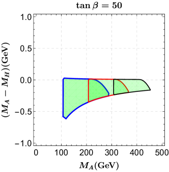
Figure 1: Mass regions allowed in the $(M_{A},M_{A}-M_{H})$ plane by the theoretical and experimental constraints (see the text). The blue, red and black boundaries correspond to $M_{H^{\pm}}=200$, $300$ and $400$ GeV, respectively.

We should emphasize that, except for the custodial symmetry that protects $M_{A}\simeq M_{H^{\pm}}$ Pomarol and Vega (1994); Haber and O’Neil (2011) or the twisted custodial symmetry that protects $M_{H}\simeq M_{H^{\pm}}$ Gerard and Herquet (2007); Haber and O’Neil (2011), there exists no any symmetry protecting $M_{H}\simeq M_{A}$. Then, for large tree-level $M_{H}$ and $M_{A}$, the radiative self-energy corrections may generate dangerous mass splitting between $M_{H}$ and $M_{A}$, and hence violate the constraints under discussion. To this end, we require the (pseudo)scalar masses to be relatively small, e.g., $M_{H,A}\simeq 100$ GeV and $M_{H^{\pm}}\simeq 200$ GeV. Such a relatively light charged Higgs boson is also motivated by a feasible explanation for the muon $g-2$ excess under the tight constraints from the $B$-physics observables, as will be discussed in the subsequent sections.

III Muon anomalous magnetic moment in the degenerate regime

The $U(1)$ symmetry was also used to constrain the Yukawa coupling textures Li et al. (2018). Here we assume that the $U(1)$ symmetry in the quark sector is only an approximate one and allow it to be broken by an additional term in the up-quark sector, treating the coupling $Y_{1}^{u}$ as perturbation Crivellin et al. (2016) under the following $U(1)$-charge assignment: $L(Q_{Li})=0$, $L(d_{Ri})=1$, $L(u_{Ri})=-1$, $L(\Phi_{1})=0$ and $L(\Phi_{2})=-1$. Note that we do not include any perturbation in the down-quark sector, as it confronts more severe constraints from flavor physics and collider experiments Iguro and Omura (2018); Crivellin et al. (2016, 2013); Altunkaynak et al. (2015). As a consequence, the scalar-fermion interaction Lagrangian in our scenario is specified as

$$-\mathcal{L}_{\rm int} =\bar{Q}_{L}(Y_{1}^{u}\tilde{\Phi}_{1}+Y_{2}^{u}\tilde{\Phi}_{2})u_{R}+\bar{Q}_{L}Y^{d}\Phi_{2}d_{R}$$

$$+\bar{E}_{L}Y^{\ell}\Phi_{1}e_{R}+\bar{E}_{L}(Y_{1}^{\nu}\tilde{\Phi}_{1}+Y_{2}^{\nu}\tilde{\Phi}_{2})N_{R}+{\rm H.c.},$$ (4)

where $\tilde{\Phi}_{i}=i\tau_{2}\Phi_{i}^{\ast}$ with $\tau_{2}$ being the Pauli matrix; $Q_{L}$, $E_{L}$, $u_{R}$, $d_{R}$ and $e_{R}$ denote the left-handed quark and lepton doublets, the right-handed up-quark, down-quark, and charged-lepton singlets, respectively. The right-handed neutrino singlet $N_{R}$ was introduced to account for the small neutrino mass and the $R_{K^{(*)}}$ anomaly Li et al. (2018). Note that similar frameworks relevant to the muon $g-2$ are discussed in Refs. Chiang et al. (2018); Chiang and Tsumura (2018); Campos et al. (2017).

In this paper, we generalize the previously studied texture of the up-quark Yukawa coupling to

$$X^{u}_{1}\equiv\dfrac{1}{\sqrt{2}}V_{L}^{u}Y_{1}^{u}V_{R}^{u\dagger}=\left(\begin{array}[]{ccc}0&0&0\\ 0&0&\epsilon_{ct}\\ 0&\epsilon_{tc}&\epsilon_{tt}\end{array}\right),$$ (8)

where $V_{L,R}^{u}$ denote the basis transformation matrices in the up-quark sector. The Yukawa texture in Eq. (8) was studied in the general 2HDM, namely the type-III 2HDM, with or without the Cheng-Sher ansatz Iguro and Omura (2018); Li et al. (2018); Crivellin et al. (2016); Kim et al. (2015); Wang et al. (2017); Iguro and Tobe (2017); Altunkaynak et al. (2015); Crivellin et al. (2013); Chen and Nomura (2018); Cline (2016). It has been pointed out that a nonzero $\epsilon_{tc}$ can improve the discrepancy observed in $R_{D^{(*)}}$ Crivellin et al. (2016); Iguro and Tobe (2017); Li et al. (2018), while $\mathcal{O}(1)$ $\epsilon_{tt}$ is required to explain the $R_{K^{(*)}}$ anomaly Li et al. (2018). It will be shown in this section that $\mathcal{O}(1)$ $\epsilon_{tt}$ is also responsible for resolving the muon $g-2$ anomaly. On the other hand, the large contributions from $\epsilon_{tt}$ to $\bar{B}\rightarrow X_{s}\gamma$ and $B_{s}-\bar{B}_{s}$ mixing can be cancelled to a large extent, if a nonzero $\epsilon_{ct}$ is presented at the same time Crivellin et al. (2013); Altunkaynak et al. (2015); Iguro and Omura (2018); Chen and Nomura (2018), as will be discussed in Sec. IV.

In our scenario, the two crucial elements for addressing the muon $g-2$ excess are: (i) a sizeable $\epsilon_{tt}$ and (ii) a relatively light charged Higgs boson. They provide the dominant contributions to the muon $g-2$ via the typical two-loop Barr-Zee type diagrams shown in Fig. 2$(a)$ Barr and Zee (1990); Czarnecki et al. (1995); Chang et al. (2001); Cheung et al. (2001); Chen and Geng (2001); Arhrib and Baek (2002); Heinemeyer et al. (2004a, b); Abe et al. (2014); Ilisie (2015); Cherchiglia et al. (2017a) as well as the new sets of two-loop Barr-Zee type diagrams shown in Fig. 2$(b)$ Ilisie (2015). For Fig. 2$(a)$, the fermion loops come from the top quark and the $\tau$ lepton, while the bottom-quark loop has a suppression factor $1/\tan\beta$ in the large $\tan\beta$ regime and there is no neutrino loop. Note that the amplitude with the photon propagator replaced by that of the $Z$ boson is suppressed by a factor $-1/4+\sin^{2}\theta_{W}\approx-0.02$ Chang et al. (2001).

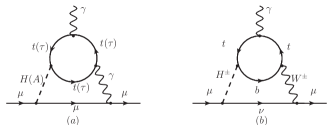
Figure 2: $(a)$: typical two-loop Barr-Zee type diagrams with the top ($\tau$) loop. $(b)$: new sets of two-loop Barr-Zee type diagrams with the top-bottom (bottom-top) loop.

As for the new sets of two-loop Barr-Zee type diagrams discussed in Ref. Ilisie (2015), we would like to make the following remarks. Due to the assumption of CP conservation in the scalar potential, there are neither $AH^{\pm}H^{\mp}$ nor $AW^{\pm}W^{\mp}$ couplings. Then, contributions from all the diagrams involving these vertices shown in Fig. 2 would vanish. Meanwhile, the contribution involving the $HH^{\pm}H^{\mp}$ vertex is suppressed in the large $\tan\beta$ regime, because the $HH^{\pm}H^{\mp}$ coupling is proportional to $1/\tan\beta$ (we have confirmed this point with the code SARAH Staub (2014)). Finally, due to the absence of the $HW^{\pm}W^{\mp}$ coupling in the SM-like limit, there exist no contributions from the diagrams involving this vertex either. Therefore, in our scenario, the diagrams shown in Fig. 2$(b)$ with the top-bottom (bottom-top) loop should give the dominant contributions among all these two-loop Barr-Zee type diagrams. We should also mention that, although the heavy neutrino with mass around the electroweak scale is introduced in our framework, we need not consider its contribution coming from Fig. 2$(b)$ with the light neutrino propagator replaced by that of the heavy neutrino $N$, because the $\mathcal{O}(1)$ $H^{\pm}N\mu^{\mp}$ coupling considered in Ref. Li et al. (2018) is compensated by the small $W^{\pm}N\mu^{\mp}$ one Antusch et al. (2006); Akhmedov et al. (2013); Fernandez-Martinez et al. (2015, 2016).

Based on these observations, we will only consider the two-loop Barr-Zee type diagrams shown in Fig. 2. The corresponding amplitudes as well as the one-loop contributions generated by the $H$, $A$ and $H^{\pm}$ propagators are collected in the Appendix. In the numerical analysis, we fix $\tan\beta=50$ and $M_{H^{\pm}}=M_{H,A}+100\leavevmode\nobreak\ {\rm GeV}$ which is allowed by the mass spectrum shown in Fig. 1. In addition, the heavy neutrino mass is fixed at $200$ GeV and an $\mathcal{O}(1)$ neutrino Yukawa coupling is adopted Li et al. (2018) (see the Appendix). The total NP contributions to the muon $g-2$ are shown in Fig. 3, where the dependence of $\Delta a_{\mu}$ on the pseudoscalar mass $M_{A}$ with different values of the top-Yukawa coupling $\epsilon_{tt}$ is displayed. It can be seen that the $1\sigma$ range of $\Delta a_{\mu}$ given by Eq. (1) can be accommodated depending on the values of the top-Yukawa coupling $\epsilon_{tt}$ and the (pseudo)scalar mass $M_{H(A)}$. For $\epsilon_{tt}=-0.5$, we obtain $30\lesssim M_{H,A}\lesssim 80$ GeV, while for $\epsilon_{tt}=-0.7$, the allowed mass region increases to $60\lesssim M_{H,A}\lesssim 160$ GeV; however, with $\epsilon_{tt}=-0.9$ and $M_{H,A}\lesssim 110$ GeV, the resulting $\Delta a_{\mu}$ would exceed the $1\sigma$ range.

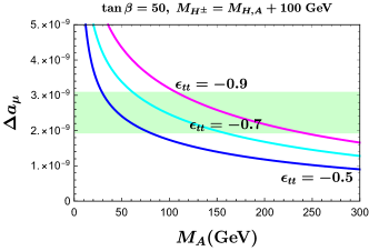
Figure 3: Dependence of $\Delta a_{\mu}$ on the pseudoscalar mass $M_{A}$ with different values of the top-Yukawa coupling $\epsilon_{tt}$. The green band corresponds to the $1\sigma$ range of $\Delta a_{\mu}$ given by Eq. (1).

It should also be mentioned that the two-loop Barr-Zee type diagrams shown in Fig. 2$(b)$ can also give a contribution to the radiative decay $\mu\rightarrow e\gamma$ if the final lepton is replaced with an electron. However, the amplitude would carry an additional factor $U_{\mu j}^{\nu}U_{ej}^{\nu*}$, where $U^{\nu}$ represents the full $6\times 6$ neutrino mixing matrix, in the convention specified in Ref. Li et al. (2018). Therefore, the amplitude would be proportional to $\sum_{j=1}^{3}U_{\mu j+1}^{\nu}U_{ej+1}^{\nu*}\equiv 2\eta_{\mu e}$, where $\eta$ represents the non-unitary effect of the neutrino mixing matrix Fernandez-Martinez et al. (2016). Following the effective Lagrangian method Crivellin et al. (2016) and taking the $2\sigma$ upper bound, $|2\eta_{\mu e}|\lesssim\mathcal{O}(10^{-5})$ Fernandez-Martinez et al. (2016), we would obtain $\mathcal{B}(\mu\rightarrow e\gamma)\lesssim\mathcal{O}(10^{-15})$, which is two orders of magnitude smaller than the current bound, $4.2\times 10^{-13}$ Baldini et al. (2016). We can, therefore, conclude that our explanation for the muon $g-2$ discrepancy does not conflict with the stringent constraint from $\mu\rightarrow e\gamma$.

IV Constraints from $B$-physics observables

In this section, we analyze the tight constraints from the $B$-physics observables, concentrating on the branching ratio of the inclusive $\bar{B}\rightarrow X_{s}\gamma$ decay and the mass difference in the $B_{s}-\bar{B}_{s}$ mixing, as the sizeable top-Yukawa coupling $\epsilon_{tt}$ and the relatively small charged Higgs boson mass give large contributions to these observables Crivellin et al. (2013); Altunkaynak et al. (2015); Iguro and Omura (2018); Chen and Nomura (2018).

IV.1 $\bar{B}\rightarrow X_{s}\gamma$

The low-energy effective Hamiltonian for the inclusive $\bar{B}\rightarrow X_{s}\gamma$ decay is given by

$$\mathcal{H}_{\rm eff}^{b\rightarrow s\gamma}=-\dfrac{4G_{F}}{\sqrt{2}}V_{ts}^{*}V_{tb}\sum_{i=1}^{8}C_{i}(\mu)\mathcal{O}_{i}(\mu),$$ (9)

where the current-current operators $\mathcal{O}_{1,2}$ and the QCD-penguin operators $\mathcal{O}_{3-6}$ could be found e.g. in Ref. Borzumati and Greub (1998), while the dipole operators $\mathcal{O}_{7\gamma}$ and $\mathcal{O}_{8g}$ are defined, respectively, as

$$\mathcal{O}_{7\gamma} =\dfrac{e}{16\pi^{2}}m_{b}\bar{s}\sigma^{\mu\nu}P_{R}bF_{\mu\nu},$$

$$\mathcal{O}_{8g} =\dfrac{g_{s}}{16\pi^{2}}m_{b}\bar{s}\sigma^{\mu\nu}P_{R}T^{a}bG^{a}_{\mu\nu}.$$ (10)

Note that the primed operators $\mathcal{O}^{\prime}_{7\gamma,8g}$ that are obtained from Eq. (10) by replacing $P_{R}$ with $P_{L}$ need not be included in Eq. (9), because the Wilson coefficients of these operators are suppressed by $m_{s}/m_{b}$ relative to those coming from $\mathcal{O}_{7\gamma,8g}$ in the SM, and are zero in our scenario due to the absence of FCNCs in the down-quark sector.

Following Ref. Buras et al. (2011), the branching ratio of the inclusive $\bar{B}\rightarrow X_{s}\gamma$ decay can be expressed as

$$\mathcal{B}(\bar{B}\rightarrow X_{s}\gamma)=R\left[|C_{7\gamma}(\mu_{b})|^{2}+N(E_{\gamma})\right],$$ (11)

where $R$ is an overall factor and determined to be $R=2.47\times 10^{-3}$ Gambino and Misiak (2001); Misiak and Steinhauser (2007), while $N(E_{\gamma})$ denotes the non-perturbative correction, with $N(E_{\gamma})=(3.6\pm 0.6)\times 10^{-3}$ Gambino and Misiak (2001) for a photon-energy cut off $E_{\gamma}>1.6$ GeV in the $\bar{B}$-meson rest frame. The Wilson coefficient $C_{7\gamma}(\mu_{b})$ can be decomposed into the sum of the SM and the NP contributions:

$$C_{7\gamma}(\mu_{b})=C^{\rm SM}_{7\gamma}(\mu_{b})+C^{\rm NP}_{7\gamma}(\mu_{b}).$$ (12)

For the SM part, we adopt the result at the next-to-next-to leading order in QCD which gives $\mathcal{B}_{s\gamma}^{\rm SM}=(3.36\pm 0.23)\times 10^{-4}$ for $E_{\gamma}>1.6$ GeV Czakon et al. (2015); Misiak et al. (2015), while for the NP contribution, we use the leading order result at the scale $\mu_{b}=\mathcal{O}(m_{b})$:

$$C^{\rm NP}_{7\gamma}(\mu_{b})=\kappa_{7}C^{\rm NP}_{7\gamma}(\mu_{H})+\kappa_{8}C^{\rm NP}_{8g}(\mu_{H}),$$ (13)

where the Wilson coefficients $C^{\rm NP}_{7\gamma}(\mu_{H})$ and $C^{\rm NP}_{8g}(\mu_{H})$ at the initial scale $\mu_{H}=\mathcal{O}(M_{H^{\pm}})$ are collected in the Appendix. For the numerical study, we take the magic numbers $\kappa_{7}=0.524$ and $\kappa_{8}=0.118$ evaluated at $\mu_{H}=200$ GeV and $\mu_{b}=2.5$ GeV Buras et al. (2011).

IV.2 $B_{s}-\bar{B}_{s}$ mixing

Adopting the overall normalization of the SM contribution, the low-energy effective Hamiltonian for $B_{s}-\bar{B}_{s}$ mixing can be written as

$$\mathcal{H}_{\rm eff}^{\Delta B=2}=\dfrac{G_{F}^{2}(V_{tb}^{*}V_{ts})^{2}}{16\pi^{2}}M_{W}^{2}\left(\sum_{i=1}^{5}C_{i}\mathcal{O}_{i}+\sum_{i=1}^{3}\tilde{C}_{i}\tilde{\mathcal{O}}_{i}\right),$$ (14)

where the four-quark operators could be found e.g. in Refs. Buras et al. (2001); Becirevic et al. (2002). In our scenario, only the Wilson coefficient $C_{1}$ of the operator

$$\mathcal{O}_{1}=\left(\bar{b}^{\alpha}\gamma_{\mu}P_{L}s^{\alpha}\right)\left(\bar{b}^{\beta}\gamma^{\mu}P_{L}s^{\beta}\right)$$ (15)

receives a significant NP contribution, while the NP contributions to the other Wilson coefficients are either absent as no FCNCs occur in the down-quark sector or suppressed by $1/\tan\beta$ in the large $\tan\beta$ regime. This can also be understood e.g. from Refs. Crivellin et al. (2013); Chen and Nomura (2018).

A prominent constraint from the $B_{s}-\bar{B}_{s}$ mixing is due to the mass difference between the two mass eigenstates of the neutral $B_{s}$ mesons which is given as $\Delta M_{s}=2|M^{s}_{12}|$, where $M_{12}^{s}$ is the off-diagonal element in the $B_{s}$-meson mass matrix, with the known SM result given by Ball and Fleischer (2006); Artuso et al. (2016); Di Luzio et al. (2018)

$$M^{s,\rm SM}_{12}=\dfrac{G_{F}^{2}}{12\pi^{2}}(V_{tb}^{*}V_{ts})^{2}M_{W}^{2}M_{B_{s}}f_{B_{s}}^{2}\hat{\eta}_{B}BS_{0}(x_{t}),$$ (16)

where $M_{B_{s}}$ and $f_{B_{s}}$ are the $B_{s}$-meson mass and decay constant, respectively. The factor $\hat{\eta}_{B}$ encodes the short-distance QCD corrections Buras et al. (1990), while the bag parameter $B$ Bazavov et al. (2016), together with the decay constant $f_{B_{s}}$, parameterizes all the long-distance QCD effect contained in the hadronic matrix element $\langle\bar{B}_{s}|\mathcal{O}_{1}|B_{s}\rangle$. Note that a different convention for the QCD correction and the bag parameter is also used in the literature through the relation $\hat{\eta}_{B}B\equiv\eta_{B}\hat{B}$ (see e.g. Ref. Aoki et al. (2017) and the relevant discussions in Refs. Lenz et al. (2011); Di Luzio et al. (2018)). The Inami-Lim function $S_{0}(x_{t}\equiv\left(\overline{m}_{t}(\overline{m}_{t})\right)^{2}/M_{W}^{2})\approx 2.39$ Inami and Lim (1981) is calculated from the $W$-boson box diagrams with two internal top-quark exchanges, the value of which is obtained with the central value of the top-quark $\overline{\rm MS}$ mass $\overline{m}_{t}(\overline{m}_{t})$ Group and Aaltonen (2016).

Normalizing to the SM contribution, we can express $\Delta M_{s}$ in the presence of NP contributions as

$$\Delta M_{s}=\Delta M_{s}^{\rm SM}|1+\Delta_{s}^{\rm NP}|,$$ (17)

where $\Delta M_{s}^{\rm SM}=(18.4^{+0.7}_{-1.2})\leavevmode\nobreak\ {\rm ps}^{-1}$ is taken from the 2019 updated result presented in Refs. Di Luzio et al. (2019); Lenz and Tetlalmatzi-Xolocotzi (2020) and $\Delta_{s}^{\rm NP}=C_{1}^{\rm NP}(\mu_{H})/(4S_{0}(x_{t}))$. The Wilson coefficient $C_{1}^{\rm NP}(\mu_{H})$ evaluated at $\mu_{H}=\mathcal{O}(M_{H^{\pm}})$ is given in the Appendix. It should be mentioned that, in obtaining Eq. (17), we have assumed that the renormalization group running effect on the NP contributions Buras et al. (2001); Becirevic et al. (2002) from the initial scale $\mu_{H}$ down to the low scale $\mu_{b}$ is identical to that in the SM part (which is encoded in the factor $\hat{\eta}_{B}$). This approximation is quite reasonable, because the charged Higgs boson mass is considered to be around the electroweak scale, being not far from the top-quark mass.

IV.3 Combined constraints from $\mathcal{B}(\bar{B}\rightarrow X_{s}\gamma)$ and $\Delta M_{s}$

We now proceed to analyze the combined constraints from the branching ratio $\mathcal{B}(\bar{B}\rightarrow X_{s}\gamma)$ and the mass difference $\Delta M_{s}$. To this end, we confront our theoretical predictions with the $1\sigma$ ranges of the world-averaged results compiled by the Heavy Flavor Averaging Group for these two observables Amhis et al. (2017): $\mathcal{B}_{s\gamma}^{\rm exp}=(3.32\pm 0.15)\times 10^{-4}$ for $E_{\gamma}>1.6$ GeV and $\Delta M_{s}^{\rm exp}=(17.757\pm 0.021)\leavevmode\nobreak\ \rm ps^{-1}$. In Fig. 4, by fixing $\epsilon_{tc}=0.1$ in light of the combined fits for $R_{D^{(*)}}$ and $B_{c}^{-}\rightarrow\tau^{-}\bar{\nu}$ Iguro and Tobe (2017); Li et al. (2018), we show the allowed parameter space in the $(\epsilon_{tt},\epsilon_{ct})$ plane, with $M_{H^{\pm}}=200$, $300$ and $400$ GeV, corresponding to the blue, red and black boundaries, respectively. We can see clearly from this figure that it is possible to allow $\epsilon_{tt}=-0.7$ and $M_{H^{\pm}}=200$ GeV even with a tightly constrained $\epsilon_{ct}$: $-0.04\lesssim\epsilon_{ct}\lesssim-0.07$. It is therefore concluded that the parameter region with large $\epsilon_{tt}$ and small $M_{H^{\pm}}$ required by the muon $g-2$ excess can still be reached under the tight constraints from these two observables.

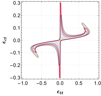
Figure 4: Allowed parameter space in the $(\epsilon_{tt},\epsilon_{ct})$ plane under the combined constraints from $\bar{B}\rightarrow X_{s}\gamma$ decay and $B_{s}-\bar{B}_{s}$ mixing. The regions with blue, red and black boundaries correspond to $M_{H^{\pm}}=200$, $300$ and $400$ GeV, respectively.

Finally, let us discuss briefly the compatibility of our scenario with the direct collider constraints. In a framework similar to what is considered here, it has been found that the neutral and charged Higgs bosons with masses being as light as 200 GeV are still compatible with the current LHC constraints Gori et al. (2018); Hou et al. (2018). For a pseudoscalar boson being lighter than the top quark, it is also found that the constraints from the top-quark decay and the same-sign top pair production at the LHC still allow $M_{A}\simeq 150$ GeV, while the 13 TeV LHC direct constraints on the charged Higgs boson mass would be weaker than those from the indirect $B$-meson physics Wang et al. (2017). More detailed analysis with scalar masses being around 200 GeV can also be found e.g. in Ref. Iguro and Tobe (2017). Regarding the LEP constraints, the current bound on the charged Higgs boson mass is $M_{H^{\pm}}>80$ GeV Abbiendi et al. (2013), while the $95\%$ C.L. lower bound of the neutral scalars is 95 GeV in the limit where $M_{H}\simeq M_{A}$ Schael et al. (2006); Cline (2016). Based on the observations, we can, therefore, conclude that the preferred region found in this paper is compatible with both the LHC and LEP constraints.

V Conclusions

In this paper, we have demonstrated that in the $U(1)$-symmetric 2HDM, where the two Higgs doublets carry different global $U(1)$ charges, the two additional neutral Higgs bosons would become nearly degenerate in the large $\tan\beta$ regime, due to the constraints from both theoretical arguments and experimental measurements. As a result, it is impossible to address the muon $g-2$ anomaly in this framework, because a significant mass splitting between the scalar and pseudoscalar Higgs bosons, as is generally required in the usual 2HDMs, cannot be realized. However, with an $\mathcal{O}(1)$ top-Yukawa coupling and a relatively light charged Higgs boson mass ($\simeq 200$ GeV), we found that there exist large contributions to the muon $g-2$ arising from the two-loop Barr-Zee type diagrams, in spite of a large cancellation between the scalar and pseudoscalar sectors, providing therefore an explanation for the muon $g-2$ excess at the $1\sigma$ level. At the same time, the required top-Yukawa coupling and charged Higgs boson mass can also survive the tight constraints from the branching ratio of the inclusive $\bar{B}\rightarrow X_{s}\gamma$ decay and the mass difference in the $B_{s}-\bar{B}_{s}$ mixing.

Appendix

In this Appendix, we collect the relevant expressions for the oblique parameters $S$, $T$ and $U$, the well-known one-loop and the two-loop Barr-Zee type contributions to the muon $g-2$, as well as the relevant Wilson coefficients in the inclusive $\bar{B}\rightarrow X_{s}\gamma$ decay and the $B_{s}-\bar{B}_{s}$ mixing, in the framework of $U(1)$-symmetric 2HDM.

V.1 Oblique parameters

Following Refs. Grimus et al. (2008); Haber and O’Neil (2011), the oblique parameters $S$, $T$ and $U$ in the SM-like limit are given, respectively, by

$$S=\frac{\left[\mathcal{B}_{22}(M_{Z}^{2},M_{H}^{2},M_{A}^{2})-\mathcal{B}_{22}(M_{Z}^{2},M_{H^{\pm}}^{2},M_{H^{\pm}}^{2})\right]}{\pi M_{Z}^{2}},$$ (18)

$$T=\dfrac{1}{16\pi\sin^{2}\theta_{W}M_{W}^{2}}\left[F\left(M_{H^{\pm}}^{2},M_{H}^{2}\right)+F\left(M_{H^{\pm}}^{2},M_{A}^{2}\right)\right.$$

$$\hskip 85.35826pt-\left.F\left(M_{H}^{2},M_{A}^{2}\right)\right],$$ (19)

$$S+U=\dfrac{1}{\pi M_{W}^{2}}\left[\mathcal{B}_{22}(M_{W}^{2},M_{H^{\pm}}^{2},M_{A}^{2})\right.$$

$$+\left.\mathcal{B}_{22}(M_{W}^{2},M_{H^{\pm}}^{2},M_{H}^{2})-2\mathcal{B}_{22}(M_{W}^{2},M_{H^{\pm}}^{2},M_{H^{\pm}}^{2})\right],$$ (20)

with

$$\mathcal{B}_{22}(q^{2},m_{1}^{2},m_{2}^{2}) =B_{22}(q^{2},m_{1}^{2},m_{2}^{2})-B_{22}(0,m_{1}^{2},m_{2}^{2}),$$ (21)

$$B_{22}(q^{2},m_{1}^{2},m_{2}^{2}) =\frac{1}{4}(\Delta+1)\left(m_{1}^{2}+m_{2}^{2}-\frac{1}{3}q^{2}\right)$$

$$-\frac{1}{2}\int^{1}_{0}dxX\ln(X-i\epsilon),$$ (22)

$$F(x,y) =\dfrac{x+y}{2}-\dfrac{xy}{x-y}\ln\left(\dfrac{x}{y}\right),$$ (23)

where $X\equiv m_{1}^{2}x+m_{2}^{2}(1-x)-q^{2}x(1-x)$, and $\Delta\equiv\frac{2}{4-d}+\ln(4\pi)-\gamma$ in $d$-dimensional space-time.

V.2 Formulas for muon $g-2$

The amplitude for the typical two-loop Barr-Zee type diagrams shown in Fig. 2$(a)$ is given by Barr and Zee (1990); Czarnecki et al. (1995); Chang et al. (2001); Cheung et al. (2001); Chen and Geng (2001); Arhrib and Baek (2002); Heinemeyer et al. (2004a, b); Abe et al. (2014); Ilisie (2015); Cherchiglia et al. (2017a)

$$\Delta a_{\mu}^{(a)} =\dfrac{G_{F}\,m_{\mu}^{2}}{4\sqrt{2}\pi^{2}}\dfrac{\alpha}{\pi}\sum_{i,f}N_{c}^{f}Q_{f}^{2}\,r_{f}^{i}\,y_{\mu}^{i}\,y_{f}^{i}\,g_{i}(r_{f}^{i}),$$ (24)

with

$$g_{i}(r_{f}^{i})=\int_{0}^{1}dx\dfrac{\mathcal{N}_{i}(x)}{x(1-x)-r_{f}^{i}}\ln\dfrac{x(1-x)}{r_{f}^{i}},$$ (25)

where $G_{F}$ is the Fermi constant and $\alpha$ the fine-structure constant; $r_{f}^{i}=m_{f}^{2}/M_{i}^{2}$ with $i=H,\,A$, and $m_{f}$, $Q_{f}$ and $N_{c}^{f}$ are the mass, the electric charge (in unit of the elementary charge), and the number of colors for fermion $f=t,\,\tau$, respectively; $\mathcal{N}_{H}(x)=2x(1-x)-1$ and $\mathcal{N}_{A}(x)=1$. In our scenario, the fermion couplings of neutral Higgs bosons are given by $y_{\mu,\tau}^{H}=-y_{\mu,\tau}^{A}=\tan\beta$ and $y_{t}^{H}=y_{t}^{A}=\dfrac{v}{m_{t}}\epsilon_{tt}$.

The amplitude for the new sets of two-loop Barr-Zee type diagrams shown in Fig. 2$(b)$ is given by Ilisie (2015); Crivellin et al. (2016)

$$\Delta a_{\mu}^{(b)} =\dfrac{\alpha\,m_{\mu}^{2}\,N_{c}\,|V_{tb}|^{2}}{32\pi^{3}\sin^{2}\theta_{W}(M_{H^{\pm}}^{2}-M_{W}^{2})}\tan\beta\dfrac{m_{t}}{v}\epsilon_{tt}$$

$$\times\int_{0}^{1}\left[Q_{t}x+Q_{b}(1-x)\right]x(1+x)$$

$$\times\left[\mathcal{G}\left(\dfrac{m_{t}^{2}}{M_{H^{\pm}}^{2}},\dfrac{m_{b}^{2}}{M_{H^{\pm}}^{2}}\right)-\mathcal{G}\left(\dfrac{m_{t}^{2}}{M_{W}^{2}},\dfrac{m_{b}^{2}}{M_{W}^{2}}\right)\right],$$ (26)

where $V_{tb}$ is the CKM matrix element, and

$$\mathcal{G}\left(r_{a},r_{b}\right)=\dfrac{\ln\left(\dfrac{r_{a}x+r_{b}(1-x)}{x(1-x)}\right)}{x(1-x)-r_{a}x-r_{b}(1-x)}.$$ (27)

The well-known one-loop amplitudes generated by the neutral and charged Higgs boson propagators are given by Barr and Zee (1990); Czarnecki et al. (1995); Chang et al. (2001); Cheung et al. (2001); Chen and Geng (2001); Arhrib and Baek (2002); Heinemeyer et al. (2004a, b); Abe et al. (2014); Ilisie (2015); Cherchiglia et al. (2017a)

$$\Delta a_{\mu}^{H,A} =\dfrac{G_{F}\,m_{\mu}^{2}}{4\sqrt{2}\pi^{2}}\tan^{2}\beta\left[\dfrac{m_{\mu}^{2}}{M_{H}^{2}}\left(-\ln\dfrac{m_{\mu}^{2}}{M_{H}^{2}}-\dfrac{7}{6}\right)\right.$$

$$+\left.\dfrac{m_{\mu}^{2}}{M_{A}^{2}}\left(\ln\dfrac{m_{\mu}^{2}}{M_{A}^{2}}+\dfrac{11}{6}\right)\right],$$ (28)

$$\Delta a_{\mu}^{H^{\pm}} =\dfrac{G_{F}\,m_{\mu}^{2}}{4\sqrt{2}\pi^{2}}\tan^{2}\beta\dfrac{m_{\mu}^{2}}{M_{H^{\pm}}^{2}}\left(-\dfrac{1}{6}\right)$$

$$+\dfrac{|x_{2}|^{2}}{16\pi^{2}}\dfrac{m_{\mu}^{2}}{M_{H^{\pm}}^{2}}\left(-\dfrac{1}{6}\right)\mathcal{J}\left(\dfrac{M^{2}}{M_{H^{\pm}}^{2}}\right),$$ (29)

with

$$\mathcal{J}(x) =\dfrac{2x^{3}+3x^{2}-6x^{2}\ln x-6x+1}{(x-1)^{4}}.$$ (30)

Note that in obtaining $\Delta a_{\mu}^{H,A}$, we have neglected the $\mathcal{O}(m_{\mu}^{4}/M_{H,A}^{4})$ terms. The first term in $\Delta a_{\mu}^{H^{\pm}}$ stems from the diagram with light neutrino propagator, while the second term from the heavy neutrino propagator Ma and Raidal (2001). In line with our previous work Li et al. (2018), we take the muon-philic coupling $x_{2}=1$ and the heavy neutrino mass $M=200$ GeV during the numerical analysis.

V.3 Wilson coefficients in $\bar{B}\rightarrow X_{s}\gamma$ decay and $B_{s}-\bar{B}_{s}$ mixing

For the inclusive $\bar{B}\rightarrow X_{s}\gamma$ decay, in our scenario, only $C_{7\gamma}^{\rm NP}(\mu_{H})$ and $C_{8g}^{\rm NP}(\mu_{H})$ get a significant NP contribution from the one-loop penguin diagram with charged Higgs boson exchange. They are given as Crivellin et al. (2013); Altunkaynak et al. (2015); Iguro and Omura (2018); Chen and Nomura (2018)

$$C_{7\gamma,8g}^{\rm NP}(\mu_{H}) =\dfrac{v^{2}}{m_{t}^{2}}\left(\dfrac{V_{cs}^{*}}{V_{ts}^{*}}\epsilon_{ct}\epsilon_{tt}+|\epsilon_{tt}|^{2}\right)E_{7,8}(y_{t})$$

$$+\dfrac{v^{2}}{m_{c}^{2}}|\epsilon_{tc}|^{2}E_{7,8}(y_{c}),$$ (31)

where $y_{t,c}\equiv m_{t,c}^{2}/M^{2}_{H^{\pm}}$, and the scalar functions $E_{7,8}$ are defined by

$$E_{7}(y) =\frac{y\left[\left(18y^{2}-12y\right)\ln y-8y^{3}+3y^{2}+12y-7\right]}{72(y-1)^{4}},$$

$$E_{8}(y) =\frac{y\left(-6y\ln y-y^{3}+6y^{2}-3y-2\right)}{24(y-1)^{4}},$$ (32)

which can be found e.g. in Refs. Borzumati and Greub (1998); Crivellin et al. (2013); Altunkaynak et al. (2015); Iguro and Omura (2018); Chen and Nomura (2018).

For the $B_{s}-\bar{B}_{s}$ mixing, in our scenario, the dominant NP contribution to the mass difference $\Delta M_{s}$ comes from the one-loop box diagrams involving the charged Higgs boson exchange, and only the Wilson coefficient $C_{1}$ is significantly affected (see the text). The total NP contributions to $C_{1}$ at the initial scale $\mu_{H}=\mathcal{O}(M_{H^{\pm}})$ can be written as

$$C_{1}^{\rm NP}(\mu_{H})=C_{1}^{HH}(\mu_{H})+C_{1}^{HW(G)}(\mu_{H}).$$ (33)

The part of $C_{1}^{\rm NP}(\mu_{H})$ from the pure charged Higgs boson box diagrams can be written as

$$C_{1}^{HH}(\mu_{H}) =-\dfrac{4v^{4}}{M_{W}^{2}}\bigg{\{}|\epsilon_{tc}|^{4}D_{00}(m_{c}^{2},m_{c}^{2},M_{H^{\pm}}^{2},M_{H^{\pm}}^{2})\bigg{.}$$

$$+\bigg{.}\dfrac{V_{cs}^{2}}{V_{ts}^{2}}\epsilon_{tt}^{2}\epsilon_{ct}^{*2}D_{00}(m_{t}^{2},m_{t}^{2},M_{H^{\pm}}^{2},M_{H^{\pm}}^{2})\bigg{.}$$

$$+\bigg{.}\dfrac{V_{cs}}{V_{ts}}\epsilon_{tt}\epsilon_{ct}^{*}|\epsilon_{tc}|^{2}\Big{[}D_{00}(m_{t}^{2},m_{c}^{2},M_{H^{\pm}}^{2},M_{H^{\pm}}^{2})\Big{.}\bigg{.}$$

$$+\bigg{.}\Big{.}D_{00}(m_{c}^{2},m_{t}^{2},M_{H^{\pm}}^{2},M_{H^{\pm}}^{2})\Big{]}\bigg{\}},$$ (34)

while the part from the $H^{\pm}$-$W^{\pm}$ and $H^{\pm}$-$G^{\pm}$ box diagrams is given by

$$C_{1}^{HW(G)}(\mu_{H}) =\dfrac{8v^{2}m_{t}^{2}}{M_{W}^{2}}\left(\dfrac{V_{cs}}{V_{ts}}\epsilon_{ct}^{*}\epsilon_{tt}+|\epsilon_{tt}|^{2}\right)$$

$$\times\Big{[}M_{W}^{2}D_{0}(M_{W}^{2},M_{H^{\pm}}^{2},m_{t}^{2},m_{t}^{2})\Big{.}$$

$$\qquad-\Big{.}D_{00}(M_{W}^{2},M_{H^{\pm}}^{2},m_{t}^{2},m_{t}^{2})\Big{]},$$ (35)

where $D_{00}(m_{1}^{2},m_{2}^{2},m_{3}^{2},m_{4}^{2})$ and $D_{0}(m_{1}^{2},m_{2}^{2},m_{3}^{2},m_{4}^{2})$ correspond to the Passarino-Veltman functions Passarino and Veltman (1979) in the FeynCalc convention Mertig et al. (1991); Shtabovenko et al. (2016). Note that the result of $C_{1}^{\rm NP}(\mu_{H})$ in our scenario can be obtained by adjusting the relevant Yukawa couplings in Ref. Crivellin et al. (2013), which is also consistent with the ones used in Refs. Altunkaynak et al. (2015); Iguro and Omura (2018); Chen and Nomura (2018).

References

- Miller et al. (2007) J. P. Miller, E. de Rafael, and B. L. Roberts, Rept. Prog. Phys. 70, 795 (2007), arXiv:hep-ph/0703049 [hep-ph] .
- Jegerlehner and Nyffeler (2009) F. Jegerlehner and A. Nyffeler, Phys. Rept. 477, 1 (2009), arXiv:0902.3360 [hep-ph] .
- Miller et al. (2012) J. P. Miller, E. de Rafael, B. L. Roberts, and D. Stöckinger, Ann. Rev. Nucl. Part. Sci. 62, 237 (2012).
- Lindner et al. (2018) M. Lindner, M. Platscher, and F. S. Queiroz, Phys. Rept. 731, 1 (2018), arXiv:1610.06587 [hep-ph] .
- Jegerlehner (2017) F. Jegerlehner, Springer Tracts Mod. Phys. 274, pp.1 (2017).
- Aoyama et al. (2020) T. Aoyama et al., Phys. Rept. 887, 1 (2020), arXiv:2006.04822 [hep-ph] .
- Bennett et al. (2006) G. W. Bennett et al. (Muon g-2), Phys. Rev. D73, 072003 (2006), arXiv:hep-ex/0602035 [hep-ex] .
- Grange et al. (2015) J. Grange et al. (Muon g-2), (2015), arXiv:1501.06858 [physics.ins-det] .
- Abi et al. (2021) B. Abi et al. (Muon g-2), Phys. Rev. Lett. 126, 141801 (2021), arXiv:2104.03281 [hep-ex] .
- Abe et al. (2019) M. Abe et al., PTEP 2019, 053C02 (2019), arXiv:1901.03047 [physics.ins-det] .
- Gunion et al. (2000) J. F. Gunion, H. E. Haber, G. L. Kane, and S. Dawson, Front. Phys. 80, 1 (2000).
- Branco et al. (2012) G. C. Branco, P. M. Ferreira, L. Lavoura, M. N. Rebelo, M. Sher, and J. P. Silva, Phys. Rept. 516, 1 (2012), arXiv:1106.0034 [hep-ph] .
- Cheung and Kong (2003) K. Cheung and O. C. W. Kong, Phys. Rev. D68, 053003 (2003), arXiv:hep-ph/0302111 [hep-ph] .
- Broggio et al. (2014) A. Broggio, E. J. Chun, M. Passera, K. M. Patel, and S. K. Vempati, JHEP 11, 058 (2014), arXiv:1409.3199 [hep-ph] .
- Misiak and Steinhauser (2017) M. Misiak and M. Steinhauser, Eur. Phys. J. C77, 201 (2017), arXiv:1702.04571 [hep-ph] .
- Mahmoudi and Stal (2010) F. Mahmoudi and O. Stal, Phys. Rev. D81, 035016 (2010), arXiv:0907.1791 [hep-ph] .
- Deschamps et al. (2010) O. Deschamps, S. Descotes-Genon, S. Monteil, V. Niess, S. T’Jampens, and V. Tisserand, Phys. Rev. D82, 073012 (2010), arXiv:0907.5135 [hep-ph] .
- Coleppa et al. (2014) B. Coleppa, F. Kling, and S. Su, JHEP 01, 161 (2014), arXiv:1305.0002 [hep-ph] .
- Eberhardt et al. (2013) O. Eberhardt, U. Nierste, and M. Wiebusch, JHEP 07, 118 (2013), arXiv:1305.1649 [hep-ph] .
- Belanger et al. (2013) G. Belanger, B. Dumont, U. Ellwanger, J. F. Gunion, and S. Kraml, Phys. Rev. D88, 075008 (2013), arXiv:1306.2941 [hep-ph] .
- Celis et al. (2013) A. Celis, V. Ilisie, and A. Pich, JHEP 12, 095 (2013), arXiv:1310.7941 [hep-ph] .
- Chowdhury and Eberhardt (2018) D. Chowdhury and O. Eberhardt, JHEP 05, 161 (2018), arXiv:1711.02095 [hep-ph] .
- Haller et al. (2018) J. Haller, A. Hoecker, R. Kogler, K. Mönig, T. Peiffer, and J. Stelzer, (2018), arXiv:1803.01853 [hep-ph] .
- Wang and Han (2015) L. Wang and X.-F. Han, JHEP 05, 039 (2015), arXiv:1412.4874 [hep-ph] .
- Abe et al. (2015) T. Abe, R. Sato, and K. Yagyu, JHEP 07, 064 (2015), arXiv:1504.07059 [hep-ph] .
- Chun and Kim (2016) E. J. Chun and J. Kim, JHEP 07, 110 (2016), arXiv:1605.06298 [hep-ph] .
- Omura et al. (2015) Y. Omura, E. Senaha, and K. Tobe, JHEP 05, 028 (2015), arXiv:1502.07824 [hep-ph] .
- Omura et al. (2016) Y. Omura, E. Senaha, and K. Tobe, Phys. Rev. D94, 055019 (2016), arXiv:1511.08880 [hep-ph] .
- Chiang et al. (2016) C.-W. Chiang, K. Fuyuto, and E. Senaha, Phys. Lett. B762, 315 (2016), arXiv:1607.07316 [hep-ph] .
- Iguro and Omura (2018) S. Iguro and Y. Omura, JHEP 05, 173 (2018), arXiv:1802.01732 [hep-ph] .
- Han et al. (2016) T. Han, S. K. Kang, and J. Sayre, JHEP 02, 097 (2016), arXiv:1511.05162 [hep-ph] .
- Ilisie (2015) V. Ilisie, JHEP 04, 077 (2015), arXiv:1502.04199 [hep-ph] .
- Cherchiglia et al. (2017a) A. Cherchiglia, P. Kneschke, D. Stckinger, and H. Stckinger-Kim, JHEP 01, 007 (2017a), arXiv:1607.06292 [hep-ph] .
- Cherchiglia et al. (2017b) A. Cherchiglia, D. Stckinger, and H. Stckinger-Kim, (2017b), arXiv:1711.11567 [hep-ph] .
- Li et al. (2018) S.-P. Li, X.-Q. Li, Y.-D. Yang, and X. Zhang, (2018), arXiv:1807.08530 [hep-ph] .
- Lees et al. (2012) J. P. Lees et al. (BaBar), Phys. Rev. Lett. 109, 101802 (2012), arXiv:1205.5442 [hep-ex] .
- Lees et al. (2013) J. P. Lees et al. (BaBar), Phys. Rev. D88, 072012 (2013), arXiv:1303.0571 [hep-ex] .
- Huschle et al. (2015) M. Huschle et al. (Belle), Phys. Rev. D92, 072014 (2015), arXiv:1507.03233 [hep-ex] .
- Aaij et al. (2015) R. Aaij et al. (LHCb), Phys. Rev. Lett. 115, 111803 (2015), [Erratum: Phys. Rev. Lett.115,no.15,159901(2015)], arXiv:1506.08614 [hep-ex] .
- Hirose et al. (2017) S. Hirose et al. (Belle), Phys. Rev. Lett. 118, 211801 (2017), arXiv:1612.00529 [hep-ex] .
- Sato et al. (2016) Y. Sato et al. (Belle), Phys. Rev. D94, 072007 (2016), arXiv:1607.07923 [hep-ex] .
- Hirose et al. (2018) S. Hirose et al. (Belle), Phys. Rev. D97, 012004 (2018), arXiv:1709.00129 [hep-ex] .
- Aaij et al. (2018a) R. Aaij et al. (LHCb), Phys. Rev. Lett. 120, 171802 (2018a), arXiv:1708.08856 [hep-ex] .
- Aaij et al. (2018b) R. Aaij et al. (LHCb), Phys. Rev. D97, 072013 (2018b), arXiv:1711.02505 [hep-ex] .
- Aaij et al. (2014) R. Aaij et al. (LHCb), Phys. Rev. Lett. 113, 151601 (2014), arXiv:1406.6482 [hep-ex] .
- Aaij et al. (2017) R. Aaij et al. (LHCb), JHEP 08, 055 (2017), arXiv:1705.05802 [hep-ex] .
- Esteban et al. (2017) I. Esteban, M. C. Gonzalez-Garcia, M. Maltoni, I. Martinez-Soler, and T. Schwetz, JHEP 01, 087 (2017), arXiv:1611.01514 [hep-ph] .
- Capozzi et al. (2017) F. Capozzi, E. Di Valentino, E. Lisi, A. Marrone, A. Melchiorri, and A. Palazzo, Phys. Rev. D95, 096014 (2017), arXiv:1703.04471 [hep-ph] .
- de Salas et al. (2018) P. F. de Salas, D. V. Forero, C. A. Ternes, M. Tortola, and J. W. F. Valle, Phys. Lett. B782, 633 (2018), arXiv:1708.01186 [hep-ph] .
- Crivellin et al. (2016) A. Crivellin, J. Heeck, and P. Stoffer, Phys. Rev. Lett. 116, 081801 (2016), arXiv:1507.07567 [hep-ph] .
- Barr and Zee (1990) S. M. Barr and A. Zee, Phys. Rev. Lett. 65, 21 (1990), [Erratum: Phys. Rev. Lett.65,2920(1990)].
- Czarnecki et al. (1995) A. Czarnecki, B. Krause, and W. J. Marciano, Phys. Rev. D52, R2619 (1995), arXiv:hep-ph/9506256 [hep-ph] .
- Chang et al. (2001) D. Chang, W.-F. Chang, C.-H. Chou, and W.-Y. Keung, Phys. Rev. D63, 091301 (2001), arXiv:hep-ph/0009292 [hep-ph] .
- Cheung et al. (2001) K.-m. Cheung, C.-H. Chou, and O. C. W. Kong, Phys. Rev. D64, 111301 (2001), arXiv:hep-ph/0103183 [hep-ph] .
- Chen and Geng (2001) C.-H. Chen and C. Q. Geng, Phys. Lett. B511, 77 (2001), arXiv:hep-ph/0104151 [hep-ph] .
- Arhrib and Baek (2002) A. Arhrib and S. Baek, Phys. Rev. D65, 075002 (2002), arXiv:hep-ph/0104225 [hep-ph] .
- Heinemeyer et al. (2004a) S. Heinemeyer, D. Stockinger, and G. Weiglein, Nucl. Phys. B690, 62 (2004a), arXiv:hep-ph/0312264 [hep-ph] .
- Heinemeyer et al. (2004b) S. Heinemeyer, D. Stockinger, and G. Weiglein, Nucl. Phys. B699, 103 (2004b), arXiv:hep-ph/0405255 [hep-ph] .
- Abe et al. (2014) T. Abe, J. Hisano, T. Kitahara, and K. Tobioka, JHEP 01, 106 (2014), [Erratum: JHEP04,161(2016)], arXiv:1311.4704 [hep-ph] .
- Gunion and Haber (2003) J. F. Gunion and H. E. Haber, Phys. Rev. D67, 075019 (2003), arXiv:hep-ph/0207010 [hep-ph] .
- Craig et al. (2013) N. Craig, J. Galloway, and S. Thomas, (2013), arXiv:1305.2424 [hep-ph] .
- Carena et al. (2014) M. Carena, I. Low, N. R. Shah, and C. E. M. Wagner, JHEP 04, 015 (2014), arXiv:1310.2248 [hep-ph] .
- Bhupal Dev and Pilaftsis (2014) P. S. Bhupal Dev and A. Pilaftsis, JHEP 12, 024 (2014), [Erratum: JHEP11,147(2015)], arXiv:1408.3405 [hep-ph] .
- Bernon et al. (2015) J. Bernon, J. F. Gunion, H. E. Haber, Y. Jiang, and S. Kraml, Phys. Rev. D92, 075004 (2015), arXiv:1507.00933 [hep-ph] .
- Grzadkowski et al. (2018) B. Grzadkowski, H. E. Haber, O. M. Ogreid, and P. Osland, (2018), arXiv:1808.01472 [hep-ph] .
- Kanemura et al. (2004) S. Kanemura, Y. Okada, E. Senaha, and C. P. Yuan, Phys. Rev. D70, 115002 (2004), arXiv:hep-ph/0408364 [hep-ph] .
- Kanemura et al. (1993) S. Kanemura, T. Kubota, and E. Takasugi, Phys. Lett. B313, 155 (1993), arXiv:hep-ph/9303263 [hep-ph] .
- Akeroyd et al. (2000) A. G. Akeroyd, A. Arhrib, and E.-M. Naimi, Phys. Lett. B490, 119 (2000), arXiv:hep-ph/0006035 [hep-ph] .
- Ginzburg and Ivanov (2005) I. F. Ginzburg and I. P. Ivanov, Phys. Rev. D72, 115010 (2005), arXiv:hep-ph/0508020 [hep-ph] .
- Horejsi and Kladiva (2006) J. Horejsi and M. Kladiva, Eur. Phys. J. C46, 81 (2006), arXiv:hep-ph/0510154 [hep-ph] .
- Cacchio et al. (2016) V. Cacchio, D. Chowdhury, O. Eberhardt, and C. W. Murphy, JHEP 11, 026 (2016), arXiv:1609.01290 [hep-ph] .
- Grimus et al. (2008) W. Grimus, L. Lavoura, O. M. Ogreid, and P. Osland, Nucl. Phys. B801, 81 (2008), arXiv:0802.4353 [hep-ph] .
- Haber and O’Neil (2011) H. E. Haber and D. O’Neil, Phys. Rev. D83, 055017 (2011), arXiv:1011.6188 [hep-ph] .
- Zyla et al. (2020) P. A. Zyla et al. (Particle Data Group), PTEP 2020, 083C01 (2020).
- Bhattacharyya et al. (2013) G. Bhattacharyya, D. Das, P. B. Pal, and M. N. Rebelo, JHEP 10, 081 (2013), arXiv:1308.4297 [hep-ph] .
- Bhattacharyya and Das (2016) G. Bhattacharyya and D. Das, Pramana 87, 40 (2016), arXiv:1507.06424 [hep-ph] .
- Pomarol and Vega (1994) A. Pomarol and R. Vega, Nucl. Phys. B413, 3 (1994), arXiv:hep-ph/9305272 [hep-ph] .
- Gerard and Herquet (2007) J. M. Gerard and M. Herquet, Phys. Rev. Lett. 98, 251802 (2007), arXiv:hep-ph/0703051 [HEP-PH] .
- Crivellin et al. (2013) A. Crivellin, A. Kokulu, and C. Greub, Phys. Rev. D87, 094031 (2013), arXiv:1303.5877 [hep-ph] .
- Altunkaynak et al. (2015) B. Altunkaynak, W.-S. Hou, C. Kao, M. Kohda, and B. McCoy, Phys. Lett. B751, 135 (2015), arXiv:1506.00651 [hep-ph] .
- Chiang et al. (2018) C.-W. Chiang, M. Takeuchi, P.-Y. Tseng, and T. T. Yanagida, (2018), arXiv:1807.00593 [hep-ph] .
- Chiang and Tsumura (2018) C.-W. Chiang and K. Tsumura, JHEP 05, 069 (2018), arXiv:1712.00574 [hep-ph] .
- Campos et al. (2017) M. D. Campos, D. Cogollo, M. Lindner, T. Melo, F. S. Queiroz, and W. Rodejohann, JHEP 08, 092 (2017), arXiv:1705.05388 [hep-ph] .
- Kim et al. (2015) C. S. Kim, Y. W. Yoon, and X.-B. Yuan, JHEP 12, 038 (2015), arXiv:1509.00491 [hep-ph] .
- Wang et al. (2017) L. Wang, J. M. Yang, and Y. Zhang, Nucl. Phys. B924, 47 (2017), arXiv:1610.05681 [hep-ph] .
- Iguro and Tobe (2017) S. Iguro and K. Tobe, Nucl. Phys. B925, 560 (2017), arXiv:1708.06176 [hep-ph] .
- Chen and Nomura (2018) C.-H. Chen and T. Nomura, (2018), arXiv:1803.00171 [hep-ph] .
- Cline (2016) J. M. Cline, Phys. Rev. D93, 075017 (2016), arXiv:1512.02210 [hep-ph] .
- Staub (2014) F. Staub, Comput. Phys. Commun. 185, 1773 (2014), arXiv:1309.7223 [hep-ph] .
- Antusch et al. (2006) S. Antusch, C. Biggio, E. Fernandez-Martinez, M. B. Gavela, and J. Lopez-Pavon, JHEP 10, 084 (2006), arXiv:hep-ph/0607020 [hep-ph] .
- Akhmedov et al. (2013) E. Akhmedov, A. Kartavtsev, M. Lindner, L. Michaels, and J. Smirnov, JHEP 05, 081 (2013), arXiv:1302.1872 [hep-ph] .
- Fernandez-Martinez et al. (2015) E. Fernandez-Martinez, J. Hernandez-Garcia, J. Lopez-Pavon, and M. Lucente, JHEP 10, 130 (2015), arXiv:1508.03051 [hep-ph] .
- Fernandez-Martinez et al. (2016) E. Fernandez-Martinez, J. Hernandez-Garcia, and J. Lopez-Pavon, JHEP 08, 033 (2016), arXiv:1605.08774 [hep-ph] .
- Baldini et al. (2016) A. M. Baldini et al. (MEG), Eur. Phys. J. C76, 434 (2016), arXiv:1605.05081 [hep-ex] .
- Borzumati and Greub (1998) F. Borzumati and C. Greub, Phys. Rev. D58, 074004 (1998), arXiv:hep-ph/9802391 [hep-ph] .
- Buras et al. (2011) A. J. Buras, L. Merlo, and E. Stamou, JHEP 08, 124 (2011), arXiv:1105.5146 [hep-ph] .
- Gambino and Misiak (2001) P. Gambino and M. Misiak, Nucl. Phys. B611, 338 (2001), arXiv:hep-ph/0104034 [hep-ph] .
- Misiak and Steinhauser (2007) M. Misiak and M. Steinhauser, Nucl. Phys. B764, 62 (2007), arXiv:hep-ph/0609241 [hep-ph] .
- Czakon et al. (2015) M. Czakon, P. Fiedler, T. Huber, M. Misiak, T. Schutzmeier, and M. Steinhauser, JHEP 04, 168 (2015), arXiv:1503.01791 [hep-ph] .
- Misiak et al. (2015) M. Misiak et al., Phys. Rev. Lett. 114, 221801 (2015), arXiv:1503.01789 [hep-ph] .
- Buras et al. (2001) A. J. Buras, S. Jager, and J. Urban, Nucl. Phys. B605, 600 (2001), arXiv:hep-ph/0102316 [hep-ph] .
- Becirevic et al. (2002) D. Becirevic, M. Ciuchini, E. Franco, V. Gimenez, G. Martinelli, A. Masiero, M. Papinutto, J. Reyes, and L. Silvestrini, Nucl. Phys. B634, 105 (2002), arXiv:hep-ph/0112303 [hep-ph] .
- Ball and Fleischer (2006) P. Ball and R. Fleischer, Eur. Phys. J. C48, 413 (2006), arXiv:hep-ph/0604249 [hep-ph] .
- Artuso et al. (2016) M. Artuso, G. Borissov, and A. Lenz, Rev. Mod. Phys. 88, 045002 (2016), arXiv:1511.09466 [hep-ph] .
- Di Luzio et al. (2018) L. Di Luzio, M. Kirk, and A. Lenz, Phys. Rev. D97, 095035 (2018), arXiv:1712.06572 [hep-ph] .
- Buras et al. (1990) A. J. Buras, M. Jamin, and P. H. Weisz, Nucl. Phys. B347, 491 (1990).
- Bazavov et al. (2016) A. Bazavov et al. (Fermilab Lattice, MILC), Phys. Rev. D93, 113016 (2016), arXiv:1602.03560 [hep-lat] .
- Aoki et al. (2017) S. Aoki et al., Eur. Phys. J. C77, 112 (2017), arXiv:1607.00299 [hep-lat] .
- Lenz et al. (2011) A. Lenz, U. Nierste, J. Charles, S. Descotes-Genon, A. Jantsch, C. Kaufhold, H. Lacker, S. Monteil, V. Niess, and S. T’Jampens, Phys. Rev. D83, 036004 (2011), arXiv:1008.1593 [hep-ph] .
- Inami and Lim (1981) T. Inami and C. S. Lim, Prog. Theor. Phys. 65, 297 (1981), [Erratum: Prog. Theor. Phys.65,1772(1981)].
- Group and Aaltonen (2016) T. E. W. Group and T. Aaltonen (CD and D0), (2016), arXiv:1608.01881 [hep-ex] .
- Di Luzio et al. (2019) L. Di Luzio, M. Kirk, A. Lenz, and T. Rauh, JHEP 12, 009 (2019), arXiv:1909.11087 [hep-ph] .
- Lenz and Tetlalmatzi-Xolocotzi (2020) A. Lenz and G. Tetlalmatzi-Xolocotzi, JHEP 07, 177 (2020), arXiv:1912.07621 [hep-ph] .
- Amhis et al. (2017) Y. Amhis et al. (HFLAV), Eur. Phys. J. C77, 895 (2017), arXiv:1612.07233 [hep-ex] .
- Gori et al. (2018) S. Gori, C. Grojean, A. Juste, and A. Paul, JHEP 01, 108 (2018), arXiv:1710.03752 [hep-ph] .
- Hou et al. (2018) W.-S. Hou, M. Kohda, and T. Modak, Phys. Lett. B786, 212 (2018), arXiv:1808.00333 [hep-ph] .
- Abbiendi et al. (2013) G. Abbiendi et al. (LEP, DELPHI, OPAL, ALEPH, L3), Eur. Phys. J. C73, 2463 (2013), arXiv:1301.6065 [hep-ex] .
- Schael et al. (2006) S. Schael et al. (DELPHI, OPAL, ALEPH, LEP Working Group for Higgs Boson Searches, L3), Eur. Phys. J. C47, 547 (2006), arXiv:hep-ex/0602042 [hep-ex] .
- Ma and Raidal (2001) E. Ma and M. Raidal, Phys. Rev. Lett. 87, 011802 (2001), [Erratum: Phys. Rev. Lett.87,159901(2001)], arXiv:hep-ph/0102255 [hep-ph] .
- Passarino and Veltman (1979) G. Passarino and M. J. G. Veltman, Nucl. Phys. B160, 151 (1979).
- Mertig et al. (1991) R. Mertig, M. Bohm, and A. Denner, Comput. Phys. Commun. 64, 345 (1991).
- Shtabovenko et al. (2016) V. Shtabovenko, R. Mertig, and F. Orellana, Comput. Phys. Commun. 207, 432 (2016), arXiv:1601.01167 [hep-ph] .