Role of intermediate continuum states in exterior complex scaling calculations of two-photon ionization cross section

Abstract

The calculation of partial two-photon ionization cross sections in the above-threshold energy region is discussed in the framework of exterior complex scaling. It is shown that with a minor modification of the usual procedure, which is based on the calculation of the outgoing partial waves of the second-order scattering wave function, reliable partial ionization amplitudes can be obtained. The modified procedure relies on a few-term least-squares fit of radial functions pertaining to different partial waves. To test the procedure, partial and total two-photon ionization cross sections of the helium atom have been calculated for a broad range of incident photon energies. The calculated cross sections may be seen to agree well with the results found in the literature. Furthermore, it is shown that, using a similar approach, partial photoionization cross sections of an atom in an autoionizing (resonance) state may be calculated in a relatively straightforward way. Such photoionization cross sections may find their use in enhanced few-parameter models describing the atom-light interaction in cases where a direct solution of the time-dependent Schrödinger equation becomes too resource-intensive.

I Introduction

Continuum-continuum transitions often play an important role in photoionization of atoms when using short-wavelength radiation from intense coherent light sources operating in the extreme ultraviolet or x-ray spectral regions, such as free electron lasers (FELs) or high-order harmonic generation (HHG) sources; when the incident flux is high enough, so that the probability for multiphoton ionization becomes non-negligible, continuum states may be encountered as both intermediate and final states of the multiphoton transition process. While the presence of resonance (autoionizing) intermediate and final states poses a computational challenge, techniques based on the method of exterior complex scaling (ECS) Simon (1979); Rescigno et al. (1997); Kurasov et al. (1994); McCurdy and Martín (2004) seem to tackle the description of both non-structured and resonant atomic continuum in a particularly efficient and elegant way.

ECS-based methods have been used in the calculations of ionization amplitudes and cross sections, e.g., for one- and two-photon single and double ionization of He McCurdy et al. (2004); Horner et al. (2007, 2008a, 2008b), as well as in time-dependent calculations, in which effective partial ionization cross sections have been extracted from the wave packet Palacios et al. (2007, 2008, 2009). One of the implementations of the ECS method, the infinite-range complex scaling (irECS) Scrinzi (2010), combined with the time-dependent surface flux approach (tSurff) Tao and Scrinzi (2012), has been used to solve the time-dependent Schrödinger equation on minimal simulation volumes. Recently, irECS has been combined with the time-dependent complete-active-space self-consistent method Sato et al. (2016) and applied to strong-field ionization and high-harmonic generation in He, Be, and Ne atoms Orimo et al. (2018).

The ECS method and its implementation in terms of B-splines Bachau et al. (2001), which are also used in the present work, is described in detail in Ref. McCurdy and Martín (2004). It is based on a transformation of radial coordinates outside a sphere with a fixed radius ($R_{0}$):

$$R(r)=\begin{cases}r&;\,r\leq R_{0}\\ R_{0}+(r-R_{0})e^{i\theta}&;\,r>R_{0}\end{cases},$$ (1)

where $\theta>0$ denotes the scaling angle. By applying the ECS transformation, the Hamiltonian operator describing an atom or a molecule becomes non-Hermitian. Requiring the wave function to vanish on the ECS contour for $r\to\infty$, outgoing scattering boundary conditions are imposed McCurdy and Martín (2004). Furthermore, the spectral representation of retarded Green’s operator using the eigenpairs of the transformed Hamiltonian operator is seen to be particularly simple and convenient to implement. These properties make the ECS method suitable for a description of the atomic and molecular continuum and for calculations of transition (collision) amplitudes.

In this work, a procedure for the calculation of partial two-photon ionization amplitudes and cross sections is presented. The procedure relies on an extraction of the ionization amplitudes from the outgoing waves in the non-scaled region of space via a least-squares fit, and is applied to the case of two-photon ionization of He atoms. Furthermore, it is shown that a similar procedure may be used to calculate photoionization amplitudes of an atom in a resonance state calculated in the framework of the ECS method.

In the calculations presented in this work, 256 B-spline basis functions Bachau et al. (2001); McCurdy and Martín (2004) have been used to represent the radial parts of the single-electron wave functions. Single-electron angular momenta up to $\ell_{\mathrm{max}}=6$ have been used. Two-electron wave functions have been written using the close-coupling approach Venuti et al. (1996); Carette et al. (2013), with the expansion augmented by either B-spline functions or other correlation basis functions. Final-state channels with principal quantum numbers up to $n_{\mathrm{max}}=10$ have been used. Most of the calculations have been performed using $R_{0}=80$ a.u. and $R_{\mathrm{max}}=300$ a.u. A quadratic-linear-quadratic knot sequence has been used to achieve: (i) an accurate description of wave functions close to the origin; (ii) a good representation of the continuum in the non-scaled region of space; and (iii) an adequate description of eigen wave functions of the scaled Hamiltonian operator which are used to represent the atomic continuum for low photoelectron kinetic energies. Throughout this work, Hartree atomic units are used unless stated otherwise.

II Description of the method

II.1 Partial ionization amplitudes and cross sections

Using ECS, one can calculate partial two-photon ionization amplitudes which correspond to accessible ionization channels McCurdy and Martín (2004); McCurdy et al. (2004). These amplitudes are calculated from the solutions of the following set of driven Schrödinger equations:

$$(E_{0}+\omega-H)|\hat{\Psi}_{1}\rangle=D|\Phi_{0}\rangle,$$ (2)

$$(E_{0}+2\omega-H)|\hat{\Psi}_{2}\rangle=D|\hat{\Psi}_{1}\rangle,$$ (3)

where $H$ denotes the complex-scaled Hamiltonian operator of the free helium atom, $|\Phi_{0}\rangle$ and $E_{0}$ the (bound) initial atomic state and its energy, $\omega$ the photon energy, and $D$ the dipole operator. States $|\hat{\Psi}_{1}\rangle$ and $|\hat{\Psi}_{2}\rangle$ describe the outgoing waves of the first- and second-order scattering states usually denoted by $|\Psi^{+}_{1}\rangle$ and $|\Psi^{+}_{2}\rangle$. A transition amplitude describing a specific final-state channel for the case of two-photon ionization is then calculated by analyzing the corresponding second-order wave function, $\hat{\Psi}_{2}(\boldsymbol{r}_{1},\boldsymbol{r}_{2})$.

Solutions $|\hat{\Psi}_{1}\rangle$ and $|\hat{\Psi}_{2}\rangle$ are obtained by inverting Eqs. (2) and (3):

$$|\hat{\Psi}_{1}\rangle =\sum_{j}\frac{|\Phi_{j}\rangle\langle\Phi_{j}|D|\Phi_{0}\rangle}{E_{0}+\omega-E_{j}},$$ (4)

$$|\hat{\Psi}_{2}\rangle =\sum_{j}\frac{|\Phi_{j}\rangle\langle\Phi_{j}|D|\hat{\Psi}_{1}\rangle}{E_{0}+2\omega-E_{j}},$$ (5)

where $|\Phi_{j}\rangle$ and $\langle\Phi_{j}|$ are the $j$th right and left eigenvector of $H$, respectively, and $E_{j}$ is the (generally complex) eigenenergy which corresponds to $|\Phi_{j}\rangle$. It is to be understood that dipole matrix elements $\langle\Phi_{j}|D|\Phi_{0}\rangle$ and $\langle\Phi_{j}|D|\hat{\Psi}^{1}\rangle$ are evaluated on the ECS contour.

For above-threshold ionization (ATI), i.e., when $E_{0}+\omega$ lies in the continuum, first-order wave function $\hat{\Psi}_{1}(\boldsymbol{r}_{1},\boldsymbol{r}_{2})$ describes a state in which at least one of the electrons is not bound. The radial function associated with the continuum electron thus extends beyond the non-scaled region of space. This makes the driving term of Eq. (3) $R_{0}$-dependent. Especially in the context of two-photon double ionization treated in the framework of the ECS method Horner et al. (2007, 2008a, 2008b); Morales et al. (2009), but sometimes also for two-photon single ionization, this may be addressed by adding a small, imaginary term $i\eta$ ($\eta>0$) in the denominator of Eq. (4):

$$|\hat{\Psi}_{1}^{\eta}\rangle =\sum_{j}\frac{|\Phi_{j}\rangle\langle\Phi_{j}|D|\Phi_{0}\rangle}{E_{0}+\omega-E_{j}+i\eta},$$ (6)

$$|\hat{\Psi}_{2}^{\eta}\rangle =\sum_{j}\frac{|\Phi_{j}\rangle\langle\Phi_{j}|D|\hat{\Psi}_{1}^{\eta}\rangle}{E_{0}+2\omega-E_{j}}.$$ (7)

The inclusion of the imaginary term results in an additional exponential damping ($\sim e^{-\eta r}$) of the radial functions of the first-order solution. By choosing a suitable value of $\eta$, the amplitudes of the radial functions associated with continuum channels can be made negligibly small near the boundary of the non-scaled region of space. The partial-wave amplitudes extracted from second-order wave function $\hat{\Psi}^{\eta}_{2}(\boldsymbol{r}_{1},\boldsymbol{r}_{2})$ (near $r=R_{0}$) may be seen to vary smoothly with $\eta$ over a relatively wide interval. This allows one to extrapolate ($\eta\to 0^{+}$) their values to obtain the amplitudes of the unmodified problem. By damping the first-order wave function, however, the peaks which appear in the generalized two-photon ionization cross section for $E_{0}+\omega$ close to intermediate resonance states (resonance-enhanced ionization) are artificially broadened. Furthermore, the same applies for the contributions from the so-called core-excited resonances Shakeshaft (2007). In these cases, the broadening can not be “undone” using the limiting procedure. An alternative way to determine the partial ionization amplitudes is discussed below.

Henceforth, the focus will be on the dipole operator written in the velocity form,

$$D=\hat{\boldsymbol{e}}\cdot(\boldsymbol{p}_{1}+\boldsymbol{p}_{2}),$$ (8)

where $\boldsymbol{p}_{1}$ and $\boldsymbol{p}_{2}$ are the electron momentum operators and $\hat{\boldsymbol{e}}$ is the unit polarization vector. Below we show how, given this particular form of the dipole operator, one can extract partial ionization amplitudes from second-order state $|\hat{\Psi}_{2}\rangle$. To do this, we project $|\hat{\Psi}_{2}\rangle$ onto a subspace spanned by the states with a fixed total orbital angular momentum and spin, a fixed ion core, $\alpha\equiv(n_{1},\ell_{1})$, and a chosen angular momentum of the remaining electron ($\ell_{2}$), but make no attempt to single out the partial wave with the chosen wave number. In particular, we are not, at this stage, concerned with a projection of $\hat{\Psi}_{2}(\boldsymbol{r}_{1},\boldsymbol{r}_{2})$ onto the channel wave functions associated with specific kinetic energies of the continuum electron, which is how partial ionization amplitudes may generally be calculated. This point will be discussed further below. The projection, which shall be denoted by $|\hat{\Psi}_{2}^{\alpha\ell_{2}}\rangle$, can be written as:

$$|\hat{\Psi}_{2}^{\alpha\ell_{2}}\rangle =\sideset{}{{}^{\prime}}{\sum}_{\beta}x_{\alpha\beta}|\{\phi_{\alpha}\chi_{\beta}\}\rangle,$$ (9)

where $|\{\phi_{\alpha}\chi_{\beta}\}\rangle$ is the antisymmetric coupled two-electron basis state with a $Z=2$ hydrogen-like core ($\phi_{\alpha}$), the primed summation runs over one-electron basis states ($\chi_{\beta}$) with $\ell_{\beta}=\ell_{2}$, and $x_{\alpha\beta}$ denotes the corresponding expansion coefficient. Let us consider the case where the helium atom is initially in the ground state and the photon energy is low enough, so that $E_{0}+\omega$ and $E_{0}+2\omega$ fall between the first ($N=1$) and the second ($N=2$) ionization threshold. Two-photon ionization then proceeds through the $1s\epsilon^{\prime}p$ intermediate continuum states, where the kinetic energy of the continuum electron has been denoted by $\epsilon^{\prime}$. The $1s\epsilon\ell_{2}$ ($\ell_{2}=s,d$) continuum channels are thus accessible in the second step, where, similarly, $\epsilon$ is the kinetic energy of the photoelectron in the final state. We write the radial function associated with the continuum electron as:

$$P_{\alpha\ell_{2}}(r)=\sideset{}{{}^{\prime}}{\sum}_{\beta}x_{\alpha\beta}P_{\chi_{\beta}}(r),$$ (10)

where $P_{\chi_{\beta}}(r)/r$ is the radial part of one-electron wave function $\chi_{\beta}(\boldsymbol{r})$. In the asymptotic region, $P_{\alpha\ell_{2}}(r)$ approximately approaches a sum of outgoing radial Coulomb functions with two characteristic wave numbers $k$ and $k^{\prime}$:

$$P_{\alpha\ell_{2}}(r) \sim\mathcal{B}\big{\{}F_{\ell_{2}}(Z_{c},k;r)+iG_{\ell_{2}}(Z_{c},k;r)\big{\}}$$ (11)

$$+\mathcal{B}^{\prime}\big{\{}F_{\ell_{2}}(Z_{c},k^{\prime};r)+iG_{\ell_{2}}(Z_{c},k^{\prime};r)\big{\}}.$$

In Eq. (11), $F_{\ell_{2}}$ and $G_{\ell_{2}}$ are the regular and irregular energy-normalized radial Coulomb functions, and $\mathcal{B}$ and $\mathcal{B}^{\prime}$ are the amplitudes associated with the two partial waves. In the case of helium, $Z_{c}=Z-1$, where $Z=2$ is the nuclear charge. To see the asymptotic form is indeed approximately given by Eq. (11), one proceeds as follows. Firstly, the value of $k$ is fixed by the energy conservation condition, which is a direct consequence of Fermi’s golden rule:

$$E_{0}+2\omega=I_{1s}+\epsilon=I_{1s}+k^{2}/2.$$ (12)

Here, $I_{1s}$ is the energy of the ion core ($1s$). Secondly, the value of $k^{\prime}$ may be calculated if one takes into account that the on-shell approximation Marante et al. (2014); Jiménez-Galán et al. (2016) is valid. Since this is the case, the transition matrix elements between non-resonant (structureless) continuum states may be seen to be approximately diagonal in the energy Jiménez-Galán et al. (2016),

$$\langle 1s\epsilon^{\prime}p|D|1s\epsilon\ell_{2}\rangle\sim\delta(\epsilon^{\prime}-\epsilon),$$ (13)

which leads to the following condition for the remaining wave number in Eq. (11):

$$\epsilon\approx\epsilon^{\prime}=E_{0}+\omega-I_{1s}=k^{\prime 2}/2.$$ (14)

Amplitudes $\mathcal{B}$ and $\mathcal{B}^{\prime}$ can then be extracted from $P_{\alpha\ell_{2}}(r)$ by a least-squares fit, and the partial two-photon ionization cross section of interest is seen to be proportional to $|\mathcal{B}|^{2}$. In Fig. 1, this is illustrated for the case of the $1s\epsilon s$ ionization channel for photon energy $\omega=0.95$ a.u. (25.85 eV). As can be seen, the real and imaginary parts of $P_{\alpha\ell_{2}}(r)\equiv P_{1s,s}(r)$ are characterized by wave beats. For $r\leq R_{0}$, but at sufficiently large radii (so that the short-range correlation potential becomes negligibly small), these beats are accurately described by Eq. (11). It has been checked that, although the shape of the driving term ($D\hat{\Psi}_{1}$) depends on $R_{0}$, $P_{\alpha\ell_{2}}(r)$ remains independent of its value for $r\leq R_{0}$. Figure 2 shows the two-photon ionization cross section for $E_{0}+2\omega$ chosen in the region of the ${}^{1}\!{S}^{e}$ and ${}^{1}\!{D}^{e}$ autoionizing states below the $N=2$ ionization threshold. Good agreement between the two-photon cross section calculated using the present method and the data available in the literature has been obtained (e.g., see Ref. Sánchez et al. (1995)). The partial cross sections for each of the ionization channels have been calculated using:

$$\sigma^{(2)}_{\alpha\ell_{2},L}(\omega)=16\pi c^{-2}\omega^{-2}\sum_{M}\big{|}\mathcal{B}^{LM}_{\alpha\ell_{2}}\big{|}^{2},$$ (15)

where $\mathcal{B}^{LM}_{\alpha\ell_{2}}(k)\equiv\mathcal{B}$ is the ionization amplitude of the channel specified by $\alpha\ell_{2}$, total orbital angular momentum $L$ and its projection $M$, and wave number $k$. It has been assumed that, asymptotically, $F_{\ell_{2}}(Z_{c},k;r)\sim\sqrt{2/(\pi k)}\sin\theta_{\ell_{2}}$ and $G_{\ell_{2}}(Z_{c},k;r)\sim-\sqrt{2/(\pi k)}\cos\theta_{\ell_{2}}$, where $\theta_{\ell_{2}}=kr+(Z_{c}/k)\ln(2kr)-\ell_{2}\pi/2+\sigma_{\ell_{2}}$ is the total phase and $\sigma_{\ell_{2}}=\arg\Gamma(\ell_{2}+1-iZ_{c}/k)$ is the Coulomb phase shift.

The extracted ionization amplitudes also allow one to calculate photoelectron angular distributions (PADs). Given amplitude $\mathcal{B}^{LM}_{\alpha\ell_{2}}(k)$, the (spin-averaged) angle-dependent ionization amplitude is given by Carette et al. (2013); O’Keeffe et al. (2010, 2013):

$$\mathcal{B}^{LM}_{\alpha\ell_{2}}(k)\sum_{m_{2}}(\ell_{1},M-m_{2};\ell_{2},m_{2}|L,M)Y_{\ell_{2}m_{2}}(\hat{\boldsymbol{k}}).$$ (16)

The spherical harmonic describing the angular dependence of the electron ejection has been denoted by $Y_{\ell_{2}m_{2}}$($\hat{\boldsymbol{k}}$), and $(\ell_{1},M-m_{2};\ell_{2},m_{2}|L,M)$ is the Clebsch-Gordan coefficient for the coupling between the angular momentum of the ion core and the angular momentum of the continuum electron. The calculation of the PADs and the corresponding asymmetry parameters for one- and two-photon ionization is described in detail in Refs. Carette et al. (2013); O’Keeffe et al. (2010, 2013).

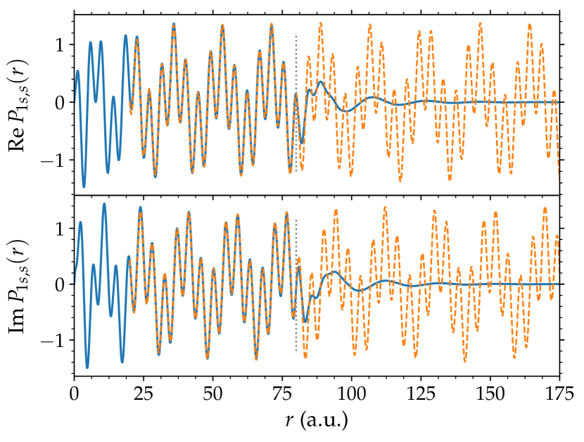
Figure 1: Real (top) and imaginary (bottom) part of the radial function for the $1s\epsilon s$ ionization channel calculated for photon energy $\omega=0.95$ a.u. (solid blue lines). Parameter $R_{0}$ has been set to 80 a.u. (marked with dotted vertical lines). The result of a least-squares fit using Eq. (11) is plotted with dashed orange lines and has been extended beyond $r=R_{0}$.

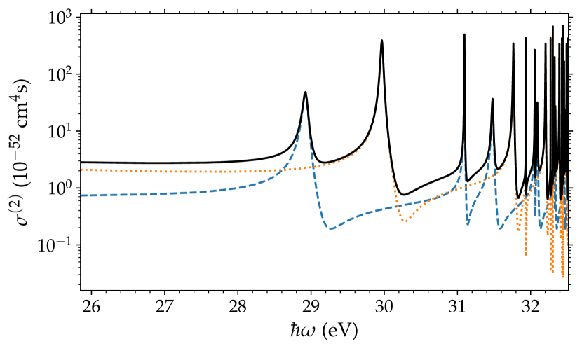
Figure 2: Two-photon ionization cross section (solid black line) in the region of the ${}^{1}\!{S}^{e}$ and ${}^{1}\!{D}^{e}$ resonance states below the $N=2$ ionization threshold. The contributions of the $1s\epsilon s$ (${}^{1}\!{S}^{e}$) and $1s\epsilon d$ (${}^{1}\!{D}^{e}$) channels are plotted with a dashed blue and a dotted orange line, respectively.

As the photon energy is further increased, but is low enough so that $E_{0}+\omega$ still lies between the $N=1$ and $N=2$ thresholds, additional final-state continuum channels become accessible, e.g., $2s\epsilon s$, $2p\epsilon p$ (${}^{1}\!{S}^{e}$ and ${}^{1}\!{D}^{e}$), etc. Let us look at the calculation of the $2p\epsilon p$ partial ionization amplitudes. The equality for $k$ now reads:

$$E_{0}+2\omega-I_{2p}=k^{2}/2.$$ (17)

In this case, however, the relation between $\epsilon$ and $\epsilon^{\prime}$ analogous to Eq. (13) is seen to be a consequence of the property of the dipole matrix element for the $1s\epsilon^{\prime}p\to 2p\epsilon p$ continuum-continuum transition, in which the continuum electron acts as a spectator:

$$\langle 1s\epsilon^{\prime}p|D|2p\epsilon p\rangle\propto{\langle\epsilon^{\prime}p|\epsilon p\rangle}\propto\delta(\epsilon^{\prime}-\epsilon).$$ (18)

This leads to the condition

$$\epsilon=\epsilon^{\prime}=k^{\prime 2}/2.$$ (19)

As before, the relevant amplitude ($\mathcal{B}$) is determined by a least-squares fit.

Finally, when the photon energy is even further increased, several (say, $K$), channels are open at energy $E_{0}+\omega$ (the first step), and $P_{\alpha\ell_{2}}(r)$ is written as a sum of at most $K+1$ terms of the form given in Eq. (11). The number of terms depends on the number of allowed continuum-continuum transitions ($n^{\prime}_{1}\ell^{\prime}_{1}\epsilon^{\prime}\ell^{\prime}_{2}\to n_{1}\ell_{1}\epsilon\ell_{2}$). The fitting procedure has been found to be stable, as long as $K$ has remained reasonably small. For photon energies above the second ionization threshold, the degeneracy in the intermediate step (e.g., for the $2s\epsilon^{\prime}p$, $2p\epsilon^{\prime}s$, and $2p\epsilon^{\prime}d$ ionization channels) has been handled by solving the normal equations using a pseudo-inverse.

It is interesting to analyze the behavior of $P_{\alpha\ell_{2}}(r)$ when $k$ coincides with one or several other wave numbers in the sum. This situation may occur, for example, for two-photon ground-state ionization through the $1s\epsilon^{\prime}p$ states in the case of the $2p\epsilon p$ channels discussed above. The resulting wave numbers are equal when

$$\epsilon=E_{0}+\omega-I_{1s}=E_{0}+2\omega-I_{2p}=\epsilon^{\prime},$$ (20)

which holds for $\omega=I_{2p}-I_{1s}$. When the photon energy lies close to $I_{2p}-I_{1s}$, the normal equations of the least-squares problem become ill-conditioned. (We discuss this further below.) This results in a resonant enhancement in the two-photon partial cross section, which is a signature of the core-excited resonance Shakeshaft (2007). A similar behavior is also present at higher photon energies, specifically, when the photon energy equals $I_{n_{1}p}-I_{1s}$. It is important to note at this point that the core-excited resonances are accessible via continuum-continuum transitions in a neutral atom (i.e., not an ion). In the present case, the relevant transitions are of the form

$$1s\epsilon^{\prime}p\to n_{1}p\epsilon p,$$ (21)

for which the continuum electron does not actively participate, as has already been mentioned. Furthermore, as has been argued by Shakeshaft Shakeshaft (2007), the present formalism for the description of two-photon ionization, in which the field-dressing (broadening) effects have not been taken into account, is not adequate for photon energies which lie very close to the positions of the core-excited resonances. A similar behavior is encountered below the ionization thresholds, when $E_{0}+\omega$ coincides with the energies of the bound $1snp$ states, unless their decay widths are taken into account. Figure 3 shows the total two-photon ionization cross section for photon energies above the $N=2$ threshold. Apart from the contributions of the final resonance states converging to higher ionization thresholds (for $\hbar\omega$ around 35 eV), a series of spikes due to the core-excited resonances is visible (centered at approximately 40.8 eV, 48.4 eV, 51.0 eV, etc.). The present result is seen to agree well with the result of Ref. Shakeshaft (2007).

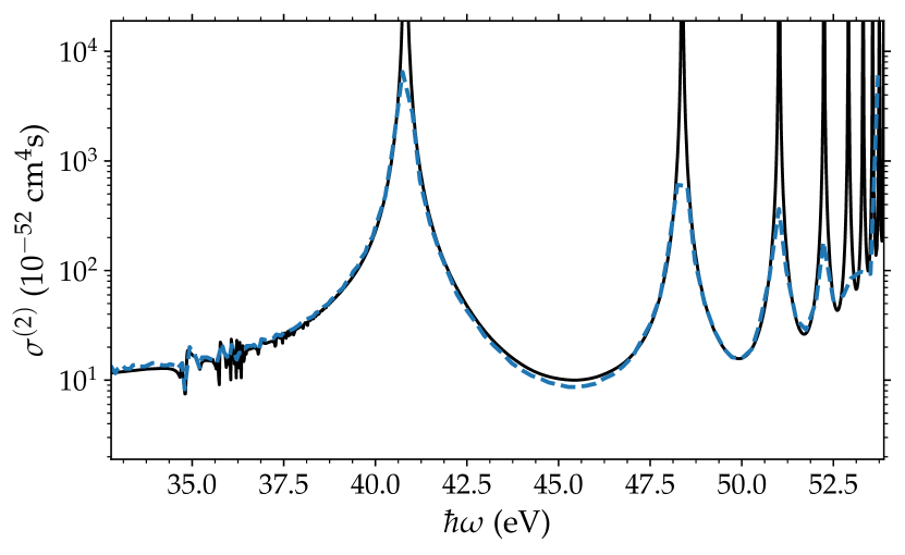
Figure 3: Two-photon ionization cross section in the region of the core-excited resonances. The result obtained using a least-squares fit with $R_{0}=80$ a.u. (solid black) and the result of Shakeshaft Shakeshaft (2007) (dashed blue) are shown.

The present approach allows one to accurately treat correlation in the initial, intermediate, and final states. In particular, electron correlation in the first- and second-order solutions, $|\hat{\Psi}_{1}\rangle$ and $|\hat{\Psi}_{2}\rangle$, is taken into account through correlated eigenstates $\langle\Phi_{j}|$ and $|\Phi_{j}\rangle$ in Eqs. (4) and (5). In the present case, electron correlation has been taken into account by including correlation basis states in the close-coupling expansion. In the current implementation, given an expansion which contains correlation wave functions and $n_{1}\ell_{1}\epsilon\ell_{2}$ continuum channel wave functions with energies of the ion core $I_{n_{1}\ell_{1}}$ up to $E_{c}$, partial ionization amplitudes for photon energies $\omega\leq(E_{c}-E_{0})/2$ can be calculated. Conversely, when the final-state energy lies above the threshold for double electron ejection, all the single-ionization channels are open. A pure close-coupling expansion has been used in this case.

Another comment is in place here concerning the structure of Eq. (3). When the photon energy lies above the ionization threshold, the radial part associated with the driving term in Eq. (3) has a “harmonic-like” form (the form of an outgoing Coulomb wave). The radial part of the Schrödinger equation thus, loosely speaking, resembles the equation of motion of a forced harmonic oscillator, with the independent variable replaced with radius $r$. For $\omega=I_{2p}-I_{1s}$ and without any additional damping, wave number $k^{\prime}$ (the “driving frequency”) matches $k$ (the “frequency of the oscillator”). This case corresponds to a resonantly driven (non-damped) harmonic oscillator. An analogous behavior for the radial function pertaining to the $2p\epsilon p$ ${}^{1}\!{S}^{e}$ channel can be seen in Fig. 4: the amplitude of the radial function increases monotonically for $r\leq R_{0}$.

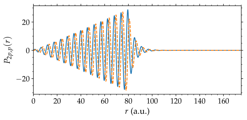
Figure 4: Radial function $P_{2p,p}(r)$ for the case of $\omega=I_{2p}-I_{1s}=0.5$ a.u. The real and imaginary part are plotted with a solid blue and dashed orange line, respectively.

As has been mentioned, the two-photon ionization cross section is enhanced when $E_{0}+\omega$ lies close to the energies of the intermediate resonance states, which is usually referred to as resonance-enhanced ionization. The resonantly enhanced two-photon ionization cross section is depicted in Fig. 5 for the case of the lowest ($N=2$) ${}^{1}\!{P}^{o}$ intermediate autoionizing states Cooper et al. (1963); Rost et al. (1997). Since these states lie between the first and the second ionization threshold, only the $1s\epsilon p$ continuum is open at $E_{0}+\omega$. As before, the wave numbers associated with the final-state ionization channels $n_{1}\ell_{1}\epsilon\ell_{2}$ are determined from $k^{2}/2=E_{0}+2\omega-I_{n_{1}\ell_{1}}$, whereas for the intermediate step, $k^{\prime 2}/2=E_{0}+\omega-I_{1s}$ is used. Similar results have also been obtained for higher-lying resonance states, including those with the energies converging to the $N=3$ ionization threshold. In the inset of Fig. 5, the total cross section in the region of the $sp_{2}^{+}$ ($2^{+}$) ${}^{1}\!{P}^{o}$ state Cooper et al. (1963) is compared to the cross section calculated using the projection to the channel wave functions (see Section II.2). The minor differences between the results calculated with the two approaches are due to the change in the background caused by the tails of the broadened nearby peaks of the core-excited resonances.

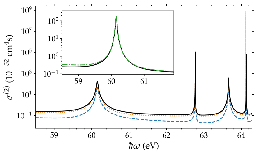
Figure 5: Resonance-enhanced two-photon ionization cross section in the energy region of the lowest ${}^{1}\!{P}^{o}$ autoionizing states. The dashed blue and dotted orange line show the contributions of the ${}^{1}\!{S}^{e}$ and ${}^{1}\!{D}^{e}$ final-state ionization channels. The total cross section is plotted with a solid black line. In the inset, the total cross section in the region of the $sp_{2}^{+}$ ${}^{1}\!{P}^{o}$ doubly-excited state is compared to the result obtained using the projection onto the final-state channel functions (green dash-dotted line), as described in Section II.2.

The least-squares procedure is also applicable in the case of two-color driving. In order to calculate the corresponding two-color ionization amplitudes, $\omega$ and $2\omega$ in Eqs. (4), (5), (12), (14), (17), and (20) should be replaced with photon energies of the two sources, $\omega_{1}$ and $\omega_{2}$. Depending on these photon energies, the resulting two-photon ionization amplitudes may be seen to correspond to the different cases studied in Ref. Jiménez-Galán et al. (2016): (i) the case of resonance-enhanced photoionization, where the final-state continuum is non-resonant; (ii) the case of two-photon ionization which proceeds through a non-resonant continuum and where the energy of the final state lies in the region of a resonance state; and (iii) the general case of doubly-resonant ionization.

II.2 Projection onto the final-state channel functions

It has been mentioned that the partial ionization amplitudes can be calculated by projecting second-order wave function $\hat{\Psi}_{2}(\boldsymbol{r}_{1},\boldsymbol{r}_{2})$ onto the channel functions which describe the continuum electron with specific kinetic energy $\epsilon$. When the ECS method is used, the projection integral is limited to the non-scaled region of space ($r\leq R_{0}$). Equivalently, the integral can be transformed to a surface integral if the form of the channel (“testing”) functions is chosen appropriately (e.g., see Refs. McCurdy et al. (2004); Palacios et al. (2007); Horner et al. (2008a)). Also in this case, the non-scaled spatial region is involved. While the peaks due to the intermediate bound or resonance states which appear in the two-photon cross section are not affected by the integration over the finite volume, the latter results in a broadening of the peaks due to the core-excited resonances. This broadening may be determined from the smallest difference between $k$ and $k^{\prime}$ which can still be resolved using the projection integral. Since $0\leq r\leq R_{0}$, this difference is given by $\Delta k=|k-k^{\prime}|\sim 2\pi/R_{0}$. For $\Delta k$ small compared to $k$ and $k^{\prime}$, the broadening may be assessed from:

$$\Delta\epsilon\approx\sqrt{2\epsilon}\,\Delta k\sim\sqrt{2\epsilon}\,\frac{2\pi}{R_{0}}.$$ (22)

Conversely, when the partial amplitudes are extracted using a fit, no additional broadening occurs. The advantage of the least-squares fit procedure is thus that it allows one to extract the partial ionization amplitudes even when $R_{0}$ is relatively low, as long as the shape of the radial function close to $r=R_{0}$ is adequately described by Eq. (11) or its multi-term generalization.

The partial two-photon ionization cross sections have been calculated by means of a projection for comparison. The ionization amplitude of the $\alpha\ell_{2}$ channel has been calculated using the following approach:

$$\mathcal{B}_{\alpha\ell_{2}} =\frac{\mathcal{I}[P_{\alpha\ell_{2}}(r)]}{\mathcal{I}[H_{\ell_{2}}(Z_{c},k;r)]},$$ (23)

$$\mathcal{I}[f(r)] =\int_{R_{\mathrm{min}}}^{R_{0}}\big{\{}H_{\ell_{2}}(Z_{c},k;r)\big{\}}^{\ast}f(r)\,w(r)dr,$$ (24)

where $H_{\ell_{2}}(Z_{c},k;r)=F_{\ell_{2}}(Z_{c},k;r)+iG_{\ell_{2}}(Z_{c},k;r)$, and a window function, denoted by $w(r)$ in Eq. (24), has been added under the integral to reduce the oscillatory artifacts. These appear due to the finite-interval (Fourier-like) side-lobes which accompany the peaks when the integrand is non-zero at the upper integral bound. The total two-photon ionization cross section in the energy region of the lowest core-excited resonance ($I_{2p}-I_{1s}=0.5\text{ a.u.}\approx 40.8$ eV) calculated with the least-squares fit (for $R_{0}=80$ a.u.) and the projection (for $R_{0}=80$ a.u., 160 a.u., 300 a.u., and 600 a.u.) is shown in Fig. 6. These results have been obtained for $R_{\mathrm{min}}=5$ a.u. and by setting $w(r)=\exp\{-(\kappa r)^{n}\}$, with $n=4$. For each of the values of $R_{0}$, parameter $\kappa$ has been calculated by requiring that $w(R_{0})=0.001$. It should be noted here that the effect of the window function is fundamentally different from the effect of the damping term ($i\eta$) in Eq. (6). While in the former case, the widths of the peaks due to the intermediate bound and resonance states remain unchanged, the peaks are artificially broadened using the latter approach. As expected, the agreement between the cross section calculated with the least-squares fit and the cross sections calculated with the projection approach is better for higher values of the $R_{0}$ parameter. It has been found that in some cases, like for the $2s\epsilon s$ channel, the partial wave amplitude approaches the asymptotic value slowly with increasing $r$ if the photon energy lies close to the energy of the core-excited resonance. In these cases, larger $R_{0}$ values have to be considered even when the amplitude is extracted using the fit.

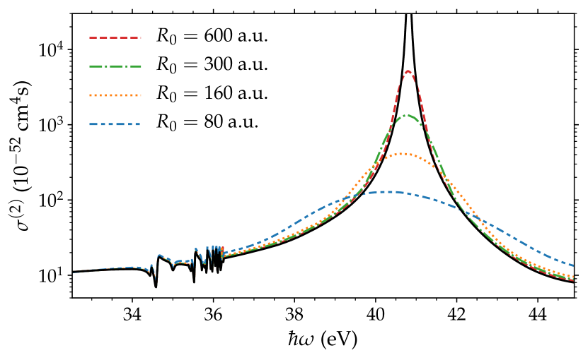
Figure 6: Two-photon ionization cross section for different scaling radii $R_{0}$ calculated with the projection approach. The cross section calculated with the least-squares fit has been plotted with a solid black line.

Equations (23) and (24) result in two-photon ionization cross sections which are almost indistinguishable from those calculated with the least-squares fit for photon energies chosen in the energy regions of intermediate bound and resonance states (as shown in the inset of Fig. 5).

A similar procedure based on a projection onto a set of channel functions is also used to extract partial single- and double-ionization amplitudes from a solution of the time-dependent Schrödinger equation (TDSE). The extraction of the ionization amplitudes from a time-dependent wave packet using the ECS method has been treated extensively by Palacios et al. Palacios et al. (2007, 2008, 2009). Let $|\Psi(t)\rangle$ denote the solution of the TDSE,

$$\big{\{}H+V(t)\big{\}}|\Psi(t)\rangle=i\frac{\partial}{\partial t}|\Psi(t)\rangle,$$ (25)

where $V(t)$ describes the interaction of the atom with an electromagnetic pulse of duration $\tau$. At the end of the pulse, the outgoing part of the wave function may be calculated from

$$(E-H)|\hat{\Psi}\rangle=|\Psi(\tau)\rangle,$$ (26)

which has the form of Eqs. (2) and (3). Partial ionization amplitudes can then be extracted from wave function $\hat{\Psi}(\boldsymbol{r}_{1},\boldsymbol{r}_{2})$, which allows one to calculate the corresponding partial ionization cross sections. As can be seen in Fig. 7, there is good overall agreement between the partial two-photon ionization cross sections calculated with the present method and the cross sections from Ref. Palacios et al. (2009), which have been obtained by solving the TDSE for 2 fs long pulses. Each of the cross sections in Fig. 7 describes an ionization process which leads to the helium ion in a specific state. These cross sections have been calculated by summing up the partial cross sections pertaining to ionization channels with a fixed ion core ($\alpha$), but with different angular momenta of the continuum electron ($\ell_{2}$) and different values of the total angular momentum ($L=0$ or $L=2$ for linearly polarized light in the present case):

$$\sigma^{(2)}_{\alpha}(\omega)=\sum_{\ell_{2},L}\sigma^{(2)}_{\alpha\ell_{2},L}(\omega).$$ (27)

The sharp peaks due to the core-excited resonances are broader in the TDSE case. As has already been mentioned, the field-broadening effects have not been taken into account in the present calculations. Furthermore, in the time-dependent treatment, additional broadening occurs due to the finite excitation bandwidth (i.e., due to the finite pulse duration). Specifically, the widths of the peaks in the TDSE case may be seen to be inversely proportional to the radial extent of the resulting wave packet (i.e., not to $R_{0}$, as in the present case). Note, however, that in Ref. Palacios et al. (2009), the value of $R_{0}$ has been chosen high enough, so that the outgoing wave packet can be assumed not to have reached the boundaries of the non-scaled spatial region for time $t\leq\tau$. Since this is the case, Eq. (22) may still be used to give the lower bound for the spectral broadening.

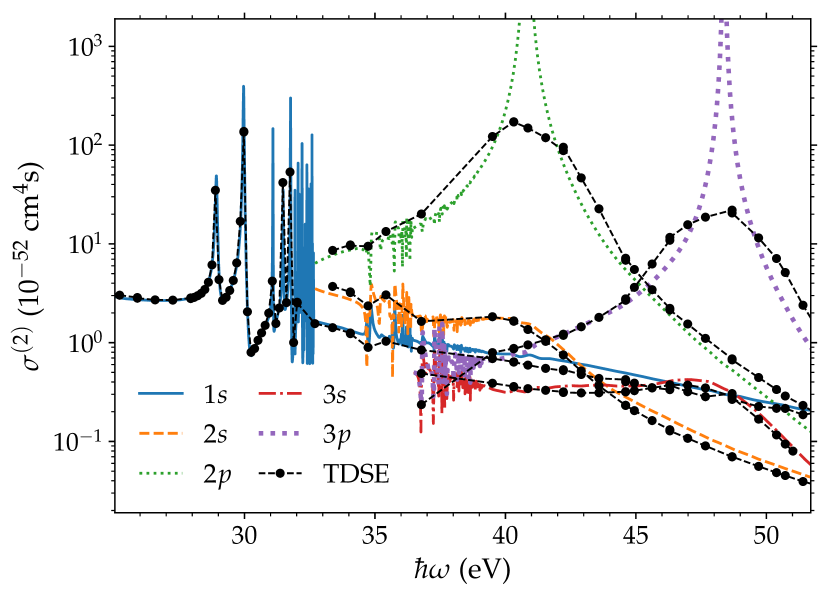
Figure 7: Partial two-photon ionization cross sections as given by Eq. (27). The $1s$, $2s$, $2p$, $3s$, and $3p$ partial cross sections are shown. The results of the time-dependent calculation (TDSE) for 2 fs long pulses (from Ref. Palacios et al. (2009)) are plotted with black circles.

Let us conclude by noting that the extraction of partial ionization amplitudes from the solution of the TDSE, i.e., from $\Psi(\boldsymbol{r}_{1},\boldsymbol{r}_{2};\tau)$, is generally not possible using the least-squares fit procedure described in this work. The reason for this is that radial function $P_{\alpha\ell_{2}}(r)$ can not generally be written in the form of Eq. (11) or its generalization, i.e., with a sum over a discrete set of wave numbers ($k,k^{\prime},\ldots$). Instead, the general form for $P_{\alpha\ell_{2}}(r)$ in the asymptotic region may be seen to be:

$$\int d{}k\,\mathcal{B}_{\alpha\ell_{2}}(k)\big{\{}F_{\ell_{2}}(Z_{c},k;r)+iG_{\ell_{2}}(Z_{c},k;r)\big{\}}.$$ (28)

The projection approach described above may in this case be used to extract $\mathcal{B}_{\alpha\ell_{2}}(k)$. The same limitations of course apply for the calculation of the PADs and energy spectra of the ejected electrons in the time-dependent framework. To this end, the following is to be noted. Energy-resolved partial two-photon ionization cross sections may be trivially calculated in the framework of the time-independent perturbation theory, and are seen to be proportional to the modulus square of the relevant partial amplitudes obtained with the least-squares fit:

$$\frac{d\sigma^{(2)}_{\alpha\ell_{2},L}}{dE}\propto\sum_{M}\big{|}\mathcal{B}^{LM}_{\alpha\ell_{2}}\big{|}^{2}\,\delta(E_{0}+2\omega-E).$$ (29)

In Eq. (29), $E=I_{\alpha}+\epsilon$ is the energy of the final state. This is in contrast to the time-dependent treatment, for which the partial amplitude can not generally be extracted from the wave packet using a fit, and photoelectron energy spectra may only be calculated by projecting $\Psi(\boldsymbol{r}_{1},\boldsymbol{r}_{2};\tau)$ onto the channel functions describing the continuum electron with a fixed kinetic energy ($\epsilon$).

II.3 Gauge invariance

Perhaps surprisingly, good agreement has been obtained between the cross sections calculated using the velocity-form and those employing the length form of the dipole operator, $D=\hat{\boldsymbol{e}}\cdot(\boldsymbol{r}_{1}+\boldsymbol{r}_{2})$, where $\boldsymbol{r}_{1}$ and $\boldsymbol{r}_{2}$ denote the position operators of the two electrons. The dipole matrix elements between the eigenstates of $H$ have been transformed to the velocity form using the well-known relation

$$\langle\Phi_{a}|\boldsymbol{p}_{1}+\boldsymbol{p}_{2}|\Phi_{b}\rangle=i(E_{a}-E_{b})\langle\Phi_{a}|\boldsymbol{r}_{1}+\boldsymbol{r}_{2}|\Phi_{b}\rangle$$ (30)

prior to calculating the first- and second-order solutions [Eqs. (4) and (5)]. In Eq. (30), eigenenergies $E_{a}$ and $E_{b}$ correspond to eigenstates $|\Phi_{a}\rangle$ and $|\Phi_{b}\rangle$, respectively. Note that Eq. (30) holds for exact eigenstates, so a discrepancy between the two forms serves as a measure of accuracy of their numerical representations. Arguably, the above relation only holds for the off-the-energy-shell matrix elements Marante et al. (2014). Note, however, that the eigenstates with different total angular momentum and parity which are used to represent the atomic continuum are non-degenerate in the present calculations. The non-degeneracy is connected to the finite radial interval used to represent the radial functions; the eigenvalues pertaining to the “box-normalized” states differ. The two-photon cross sections calculated using the length- and velocity-form of the dipole operator are shown in Fig. 8.

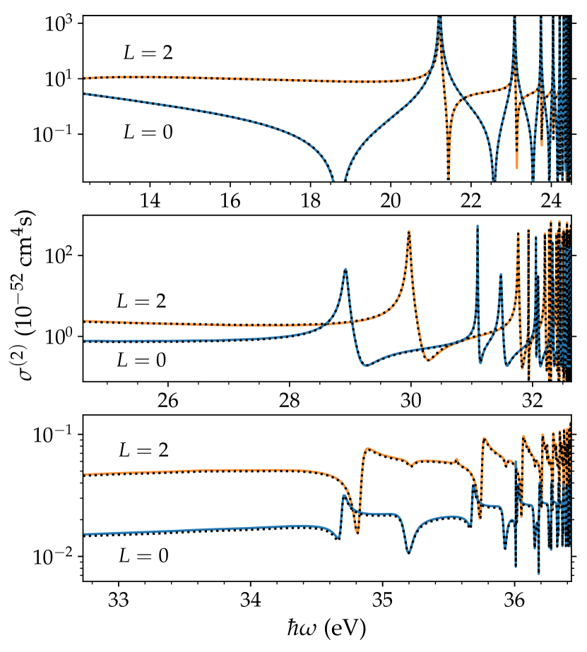
Figure 8: The ${}^{1}\!{S}^{e}$ ($L=0$) and ${}^{1}\!{D}^{e}$ ($L=2$) two-photon ionization cross section below the $N=1$ (top), $N=2$ (middle), and $N=3$ (bottom) ionization thresholds. The results for the length- and velocity-form dipole operator are plotted with solid and dotted lines, respectively.

An analogous transformation of the transition matrix elements from the acceleration to the velocity form results in spurious oscillations in the two-photon cross section even for photon energies below the first ionization threshold. The oscillations are most probably due to modifications of the commutation relations Marante et al. (2014); Mercouris et al. (1994) connecting the acceleration and velocity forms of the dipole operator, which would need to be taken into account when dealing with box-normalized states, but have not been included in the present tests.

III Photoionization of an atom in a resonance state

Theoretical treatment of photoexcitation and photoionization with short-wavelength radiation by a direct solution of the time-dependent Schrödinger equation presently becomes prohibitively lengthy as soon as the pulse duration exceeds a couple of tens of femtoseconds. When this is the case, the time-dependent description of atom-photon interaction is usually limited to a restricted subset of basis states by means of which the main features of the system can be described. This includes finding the solution of the time-dependent Schrödinger equation in terms of the time-dependent amplitudes of the basis states from the restricted space Madsen et al. (2000); Themelis et al. (2004); Mihelič et al. (2017), studying the dynamics in terms of the density matrix (e.g., see Refs. Žitnik et al. (2014); Mihelič and Žitnik (2015)), or solving a set of kinetic equations which describe the population of various atomic and ionic species during the interaction with the incident pulse Makris et al. (2009); Ilchen et al. (2016). The parameters which enter the model, such as autoionization widths, asymmetry parameters, photoionization cross sections, and Rabi frequencies, can be conveniently calculated using the ECS method. In this section, we show how to meaningfully define and calculate the photoionization cross section of an atom in a resonance state.

In the framework of the ECS method, resonance (autoionizing) states are associated with the discrete part of the eigen-spectrum of complex-scaled (ECS) Hamiltonian operator $H$, i.e., with the complex poles of the resolvent, $G(z)=(z-H)^{-1}$. Let $|\Phi_{0}\rangle$ denote an eigenstate of $H$, which represents a resonance state. Its energy can be shown to be $\theta$-independent and may be written as $E_{0}=E_{0}^{r}-i\Gamma_{0}/2$, where $E_{0}^{r}$ and $\Gamma_{0}$ denote the energy position of the resonance and its decay (autoionization) width, respectively. When the resonance is narrow, i.e., when its autoionization width is small, so that $E_{0}$ lies close to the real axis, the resonance state may be treated as a non-decaying state. In this case, we may replace $E_{0}$ in the denominator of Eq. (4) with $E_{0}^{r}$:

$$|\hat{\Psi}_{1}\rangle=\sum_{j}\frac{|\Phi_{j}\rangle\langle\Phi_{j}|D|\Phi_{0}\rangle}{E_{0}^{r}+\omega-E_{j}}.$$ (31)

As before, states $\langle\Phi_{j}|$ and $|\Phi_{j}\rangle$ denote the left and right eigenvectors of $H$, $E_{j}$ is the eigenenergy corresponding to $|\Phi_{j}\rangle$, and matrix element $\langle\Phi_{j}|D|\Phi_{0}\rangle$ is evaluated on the ECS contour.

Let us start by assuming that $|\Phi_{0}\rangle$ describes the $sp_{2}^{+}$ ${}^{1}\!{P}^{o}$ autoionizing state, which lies below the $N=2$ ionization threshold. In a similar way as before, wave number $k$ is determined from:

$$E_{0}^{r}+\omega=I_{n_{1}\ell_{1}}+\epsilon=I_{n_{1}\ell_{1}}+k^{2}/2,$$ (32)

where, again, $\alpha=(n_{1},\ell_{1})$ are the quantum numbers of the ion core for a chosen final-state channel (described by $\alpha\ell_{2}$). Contrary to the bound initial state, the $sp_{2}^{+}$ resonance state lies above the $N=1$ threshold, and thus the $1s\epsilon^{\prime}p$ continuum is open at energy $E^{r}_{0}$. Since the resonance state also contains a small admixture of the continuum Rost et al. (1997), the relation analogous to Eq. (14) now reads

$$\epsilon\approx\epsilon^{\prime}=E_{0}^{r}-I_{1s}=k^{\prime 2}/2.$$ (33)

Exactly as before, radial function $P_{\alpha\ell_{2}}(r)$ may be calculated from first-order state $|\hat{\Psi}^{\alpha\ell_{2}}_{1}\rangle$, which, in turn, is obtained by projecting the solution of Eq. (31) to the relevant subspace. In the asymptotic region, the behavior of $P_{\alpha\ell_{2}}(r)$ is approximately described by Eq. (11). In this way, the partial ionization amplitude for the $\alpha\ell_{2}$ channel can be extracted. This procedure can be generalized to higher-lying resonance states. To demonstrate its applicability, we have calculated the partial photoionization cross sections for an atom initially in the $sp_{2}^{+}$ ${}^{1}\!{P}^{o}$ autoionizing state. The results are shown in Fig. 9 for three energy regions: below the second ionization threshold, between the second and third threshold, and close to the lowest-lying core-excited resonances. As can be seen, the cross section in the latter region is enhanced in a similar way as in the case of two-photon ionization due to the continuum-continuum transitions. This enhancement occurs due to the admixture of the $1s\epsilon^{\prime}p$ continuum, i.e., due to the $1s\epsilon^{\prime}p\to np\epsilon p$ transitions. As has been the case for the two-photon ionization cross section, the field-dressing effects have not been taken into account.

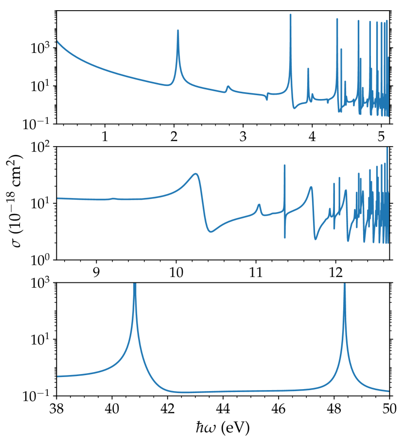
Figure 9: The photoionization cross section of the He atom in the $sp_{2}^{+}$ ${}^{1}\!{P}^{o}$ autoionizing state for the incident photon energy below the $N=2$ ionization threshold (top), between the $N=2$ and $N=3$ thresholds (middle), and in the region of the core-excited resonances (bottom).

IV Conclusion

A slightly modified procedure for the calculation of partial two-photon ionization amplitudes and cross sections based on the method of exterior complex scaling (ECS) has been presented. The procedure relies on an extraction of the amplitudes from radial functions of outgoing scattered waves obtained by fixing the state of the ion core and the angular momentum of the continuum electron. The amplitudes are not calculated by projecting out the partial waves associated with a fixed value of the kinetic energy of the electron; instead, the extraction is implemented by means of a few-term linear least-squares fit. As has become customary in the framework of the ECS method, the scattered wave is calculated by solving a set of driven Schrödinger equations. While for photon energies above the ionization threshold, the first-order driving term depends on the scaling radius, the second-order scattered wave has been seen to be independent of the scaling parameters in the non-scaled region of space. In a sense, this region contains a “complete” information on the photoionization process, and because of this, the least-squares fit allows for a relatively straightforward extraction of the photoionization amplitudes in the case of the single-electron ejection. Finally, basing on similar theoretical grounds, a method for the calculation of partial photoionization amplitudes for an atom in an autoionizing state has been proposed, which may be useful when a direct solution of the Schrödinger equation is unfeasible, and one resorts to modeling using a restricted set of states.