Scale and confinement phase transitions in scale invariant $SU(N)$ scalar gauge theory

Abstract

We consider scalegenesis, spontaneous scale symmetry breaking, by the scalar-bilinear condensation in $SU(N)$ scalar gauge theory. In an effective field theory approach to the scalar-bilinear condensation at finite temperature, we include the Polyakov loop to take into account the confinement effect. The theory with $N=3,4,5$ and $6$ is investigated, and we find that in all these cases the scale phase transition is a first-order phase transition. We also calculate the latent heat at and slightly below the critical temperature. Comparing the results with those obtained without the Polyakov loop effect, we find that the Polyakov effect can considerably increase the latent heat in some cases, which would mean a large increase in the energy density of the gravitational waves background, if it were produced by the scale phase transition.

I Introduction

The understanding of the nature of the electroweak (EW) symmetry breaking is an important subject in elementary particle physics. It is expected that the future experiments could elucidate the details of the Higgs sector. There have been many attempts to simultaneously address other important issues in the standard mode (SM) such as neutrino mass and mixing, the Baryon number asymmetry and dark matter in the Universe and also the question of what the origin of the EW scale is.

As a guide to an extension of the SM, the fact that only the Higgs mass term is dimensionful in the SM might be a hint for new physics. This question is strongly related to the so-called gauge hierarchy problem Gildener (1976); Weinberg (1979) which states why the Higgs mass is so much smaller than the Planck scale. For this issue, the scale invariance could play an important role. The mass term is set exactly equal to zero in the bare action of the SM if the scale invariance is imposed. The important fact here is that the mass term keeps vanishing along its renormalization group flow Wetterich (1984); Bardeen (1995); Aoki and Iso (2012). A mass scale corresponding to the EW symmetry breaking has to be generated by quantum effects, which we call “scalegenesis”. There are two possible ways of scalegenesis: One is known as the Coleman–Weinberg mechanism which is based on improved perturbation theory Coleman and Weinberg (1973). The other is the spontaneous scale symmetry breaking due to non-perturbative dynamics such as Quantum Chromodynamics (QCD).

Several possibilities of scalegenesis due to strong dynamics have been suggested Hur and Ko (2011); Heikinheimo et al. (2014); Holthausen et al. (2013); Kubo et al. (2014); Heikinheimo and Spethmann (2014); Carone and Ramos (2015); Ametani et al. (2015); Kubo and Yamada (2016a); Haba et al. (2016); Hatanaka et al. (2016); Ishida et al. (2017); Haba and Yamada (2017a, b); Tsumura et al. (2017); Aoki et al. (2017). One of them is based on the scalar gauge theory Kubo et al. (2014); Kubo and Yamada (2016a), where complex scalar fields $S$ coupled to a hidden $SU(N)$ gauge fields are introduced. There we have considered a situation in which the condensate $\langle S^{\dagger}S\rangle\neq 0$ of the complex scalars is formed by the strong non-abelian gauge interaction and breaks dynamically the scale invariance in the confining phase, in a similar way as the chiral condensate in QCD does. An obvious interest is to see whether or not such a vacuum state is actually realized. However, it is highly non-trivial, though not impossible Osterwalder and Seiler (1978); Fradkin and Shenker (1979), to investigate the vacua of the scalar gauge theory. For phenomenological applications of the scalar-bilinear condensate $\langle S^{\dagger}S\rangle\neq 0$, it is therefore highly desired to describe it in an effective theory. In the paper Kubo and Yamada (2016a), by mimicking the concept of the Nambu–Jona-Lasinio (NJL) model Nambu and Jona-Lasinio (1961a, b), we have attempted to formulate an effective theory. Using the mean-field approximation, we have found that the desirable vacuum structure is realized in the effective theory  Kubo and Yamada (2016a); Kubo et al. (2018). It has also turned out that the theory involves a dark matter candidate if a flavor symmetry is imposed on the scalar fields. Moreover, at finite temperature, the scale phase transition could be strongly first-order for a wide parameter space Kubo and Yamada (2015). Its signal can be observed as primordial gravitational waves Kubo and Yamada (2016b) in the future experiments such as DECIGO Seto et al. (2001); Kawamura et al. (2006, 2011) and LISA Seoane et al. (2013).

These previous works have focused on only the scalar field dynamics: The effective theory contains no gauge field, and consequently the confinement effects have been neglected. Thus, it is important to investigate the impact of confinement on the scalar dynamics, especially, on phase transitions at finite temperature. A key quantity representing the confinement is the Polyakov loop which is an order parameter for spontaneous breaking of the center symmetry of $SU(N)$ in the pure Yang–Mills theory. Effective potentials of the Polyakov loop for the pure Yang–Mills theory have been suggested to investigate the confinement–deconfinement phase transition at finite temperature Weiss (1981); Pisarski (2000); Dumitru and Pisarski (2001, 2002); Pisarski (2002); Sannino (2005); Marhauser and Pawlowski (2008); Braun et al. (2010). In the literature Fukushima (2004), the Polyakov–NJL model has been proposed in order to discuss the synergy between the chiral symmetry breaking and the confinement in QCD (see also e.g. Ratti et al. (2006); Roessner et al. (2007); Fukushima (2008); Herbst et al. (2011); Fukushima and Hatsuda (2011); Fukushima and Sasaki (2013); Fukushima and Skokov (2017)).

In this paper, following the Fukushima’s work Fukushima (2004), we study the phase transition in the effective theory for the scalar-bilinear condensation with the Polyakov loop included. In the next section we briefly explain the basic idea of the scalegenesis in the scalar gauge theory, and in the beginning part of section III, we review how the scalegenesis is described in the effective theory. In most of the early works on the Polyakov potential the $N=3$ case has been discussed from the obvious reason. Since there is no constraint on $N$ in phenomenological applications of the scalar-bilinear condensate, we start with analyzing the pure Yang–Mills theory for $N=4$, $5$, $6$ in the following part of section III. After that we include the scalar fields coupled to the Polyakov loop, which is the main part of this paper. We investigate the phase transition with the assumption that the deconfinement transition and the scale phase transition appear at the same temperature. We also calculate the latent heat that is released during the first-order phase transition in the effective theory both with the Polyakov loop included and suppressed. Needless to say that the latent heat is an important quantity that enters into the energy density of the gravitational waves background which is produced by a first-order phase transition in the early Universe. Section IV is devoted to summarize this work.

II Brief overview on scalar-condensate model

We briefly introduce the model suggested in Kubo and Yamada (2016a) and outline what has been investigated so far. We consider a hidden sector which is governed by the following $SU(N)$ scalar-gauge theory,

$${\cal L}_{\rm H} =-\frac{1}{4}F_{\mu\nu}^{a}F^{a\mu\nu}+([D^{\mu}S_{i}]^{\dagger}D_{\mu}S_{i})-\hat{\lambda}_{S}(S_{i}^{\dagger}S_{i})(S_{j}^{\dagger}S_{j})-\hat{\lambda^{\prime}}_{S}(S_{i}^{\dagger}S_{j})(S_{j}^{\dagger}S_{i})+\hat{\lambda}_{HS}(S_{i}^{\dagger}S_{i})H^{\dagger}H,$$ (1)

where $S_{i}^{a}~{}(a=1,\dots,N,~{}i=1,\dots,N_{f})$ are scalar fields in the fundamental representation of $SU(N)$, $F^{a\mu\nu}$ is the field strength of the $SU(N)$ hidden gauge field $A_{\mu}^{a}$, $D_{\mu}S_{i}=\partial_{\mu}S_{i}-igA_{\mu}^{a}S_{i}^{a}$ is the covariant derivative, and the SM Higgs doublet field is denoted by $H^{T}=(\chi_{1}+i\chi_{2},h+i\chi_{3})/\sqrt{2}$. The total Lagrangian is the sum of ${\cal L}_{\rm H}$ and ${\cal L}_{\mathrm{SM}}$, where the scalar potential of the SM part is $V_{\mathrm{SM}}=\lambda_{H}(H^{\dagger}H)^{2}$. Note that the Higgs mass term is forbidden because of classical scale invariance. We suppose in this model that below a certain energy scale the hidden gauge coupling $g$ becomes so large that the $SU(N)$ invariant scalar bilinear dynamically forms a $U(N_{f})$ invariant condensate,

$$\langle S^{\dagger}_{i}S_{j}\rangle =\left\langle\sum_{a=1}^{N}S^{a{\dagger}}_{i}S^{a}_{j}\right\rangle\propto\delta_{ij}.$$ (2)

This scalar-bilinear condensate triggers the EW symmetry breaking via the Higgs portal coupling and the Higgs mass term is generated; $m_{H}=-\hat{\lambda}_{HS}\langle S_{i}^{\dagger}S_{i}\rangle$. In other words, the origin of the EW vacuum is generated by the spontaneous scale symmetry breaking. Note here that the corresponding Nambu-Goldstone (NG) boson to the spontaneous scale symmetry breaking is dilaton. This NG boson is, however, massive since the scale symmetry is broken by the scale anomaly.

Although the idea of this model is simple, the actual analysis is highly complicated due to the non-perturbative dynamics. In the paper Kubo and Yamada (2016a), we have attempted to formulate an effective theory of (1) with the Higgs quartic interaction included: The classical scale invariance with the $U(N_{f})$ flavor symmetry uniquely singles out it to be

$${\cal L}_{\rm eff} =([\partial^{\mu}S_{i}]^{\dagger}\partial_{\mu}S_{i})-\lambda_{S}(S_{i}^{\dagger}S_{i})(S_{j}^{\dagger}S_{j})-\lambda^{\prime}_{S}(S_{i}^{\dagger}S_{j})(S_{j}^{\dagger}S_{i})+\lambda_{HS}(S_{i}^{\dagger}S_{i})H^{\dagger}H-\lambda_{H}(H^{\dagger}H)^{2},$$ (3)

and we have investigated the vacuum structure in this effective theory by using the mean-field approximation. Then the following facts have been emerged: The effective theory can describe the scalegenesis in the hidden sector, which produces the Higgs mass term in the expected way. For finite $N_{f}$ the model has a weakly interacting massive particle (WIMP), a dark matter candidate, as an excited state above the vacuum (2), and it could be tested by the future experiments of the dark matter direct detection Kubo and Yamada (2016a); Kubo et al. (2018). In the paper Kubo and Yamada (2015), the restorations of the scale and EW symmetries at finite temperature have been investigated. The scale phase transition becomes strongly first-order for a wide parameter space in the model. This scale phase transition can induce a strong first-order EW phase transition for a certain parameter choice, although the EW phase transition is weak within the SM. It has been moreover found in  Kubo and Yamada (2016b) that the released energy at the strong first-order scale phase transition can produce primordial gravitational waves which could be observed by the future space gravitational wave antennas.

In these analyses mentioned above, however, the confinement effects has not been taken into account. The purpose of the present work is to introduce the Polyakov loop into the effective theory and to investigate the impact of the confinement effects on the phase transition.

III Spontaneous Scale Symmetry Breaking and Polyakov-corrected Scale Phase Transition

III.1 At zero temperature

For a small $\lambda_{HS}\mathrel{\mathchoice{\vbox{\offinterlineskip\halign{$\m@th\displaystyle\hfil#\hfil$\cr<\crcr\sim\crcr} }}{\vbox{\offinterlineskip\halign{$\m@th\textstyle\hfil#\hfil$\cr<\crcr\sim\crcr} }}{\vbox{\offinterlineskip\halign{$\m@th\scriptstyle\hfil#\hfil$\cr<\crcr\sim\crcr} }}{\vbox{\offinterlineskip\halign{$\m@th\scriptscriptstyle\hfil#\hfil$\cr<\crcr\sim\crcr} }}}0.1$, the scale phase transition occurs at a critical temperature which is much higher than that of the EW phase transition Kubo and Yamada (2015), which means $\langle H\rangle=0$ at the scale phase transition for small values of $\lambda_{HS}$. We therefore consider the theory with the SM sector decoupled, i.e. $\lambda_{HS}=0$. The effective Lagrangian for this case is ${\cal L}_{\rm eff}$ given in (3) with $\lambda_{HS}=\lambda_{H}=0$. To obtain the effective potential in the mean-field approximation, we introduce the the auxiliary fields, $f$ and $\phi_{0}^{a}~{}(a=1,\dots,N_{f}^{2}-1)$, and rewrite the Lagrangian in such a way that the rewritten Lagrangian (the mean-field Lagrangian ${\cal L}_{\rm MFA}$) yields the equations of motion

$$f =\frac{1}{N_{f}}(S^{\dagger}_{i}S_{i}) \phi_{0}^{a} =2(S_{i}^{\dagger}t^{a}_{ij}S_{j}),$$ and (4)

where $t^{a}~{}(a=1,...,N_{f}^{2}-1)$ are the $SU(N_{f})$ generators in the fundamental representation. The desired mean-field Lagrangian is given by Kubo and Yamada (2016a)

$${\mathcal{L}}_{\text{MFA}} =([\partial^{\mu}S_{i}]^{\dagger}\partial_{\mu}S_{i})-2(N_{f}\lambda_{S}+\lambda^{\prime}_{S})f(S_{i}^{\dagger}S_{i})+N_{f}(N_{f}\lambda_{S}+\lambda^{\prime}_{S})f^{2}+\frac{\lambda_{S}^{\prime}}{2}(\phi^{a}_{0})^{2}-2\lambda_{S}^{\prime}\phi^{a}_{0}(S_{i}^{\dagger}t^{a}_{ij}S_{j}).$$ (5)

We integrate out the fluctuations $\delta S_{i}$ of $S_{i}=\bar{S}_{i}+\delta S_{i}$ around the background $\bar{S}_{i}$ in the $\overline{\mbox{MS}}$ subtraction scheme to obtain the effective potential

$$V_{\text{MFA}}\!\left(\bar{S},f\right) =\tilde{M}^{2}(\bar{S}_{i}^{\dagger}\bar{S}_{i})-N_{f}(N_{f}\lambda_{S}+\lambda^{\prime}_{S})f^{2}+\frac{NN_{f}}{32\pi^{2}}\tilde{M}^{4}\ln\frac{\tilde{M}^{2}}{\Lambda_{H}^{2}},$$ (6)

where $\Lambda_{H}=\mu e^{3/4}$ with $\mu$ being the ’t Hooft renormalization scale, and

$$\tilde{M}^{2} =2(N_{f}\lambda_{S}+\lambda^{\prime}_{S})f.$$ (7)

The absolute minimum of the potential $V_{\text{MFA}}\!\left(\bar{S},f\right)$ is found to be located at

$$\langle\bar{S}\rangle =0, \langle f\rangle =\frac{\Lambda_{H}^{2}/2}{N_{f}\lambda_{S}+\lambda_{S}^{\prime}}\exp\left(\frac{8\pi^{2}}{N(N_{f}\lambda_{S}+\lambda_{S}^{\prime})}-\frac{1}{2}\right)$$ (8)

if $N_{f}\lambda_{S}+\lambda_{S}^{\prime}>0$ is satisfied, and the minimum value of $V_{\text{MFA}}$ is given by

$$\langle V_{\text{MFA}}\rangle =-\frac{1}{16\pi^{2}}NN_{f}(N_{f}\lambda_{S}+\lambda_{S}^{\prime})^{2}\langle f\rangle^{2}<0.$$ (9)

Therefore, as long as $N_{f}\lambda_{S}+\lambda_{S}^{\prime}>0$ is satisfied, the scale symmetry is spontaneously broken by the scalar-bilinear condensate $\langle f\rangle=\langle(S_{i}^{\dagger}S_{i})\rangle$ in the effective theory.

III.2 At finite temperature

At high temperatures we expect that the scale symmetry is restored (up to anomaly) and the color degrees of freedom are no longer confined. At finite temperature $T$ the theory is equivalent to the Euclidean theory, which is periodic in the Euclidean time $x_{4}=ix^{0}$ with the period of $\beta=1/T$. The local gauge transformation has to respect this periodicity at finite temperature. In spite of this the pure gluonic action is invariant under a non-periodic (singular) gauge transformation (center symmetry Polyakov (1978); Susskind (1979); Svetitsky and Yaffe (1982); Svetitsky (1986)) defined by the transformation matrix

$$U_{k}(x_{4}) =\left({\bf 1}e^{2\pi ik/N}\right)^{x_{4}/\beta}, k =1,\dots,N-1,$$ (10)

where ${\bf 1}\exp(2\pi ik/N)$ belongs to the center of $SU(N)$, and ${\bf 1}$ is the $N\times N$ unit matrix. Under this non-periodic gauge transformation, the traced Polyakov loop in the fundamental representation

$$\ell =\frac{1}{N}\mbox{Tr}\,L$$ (11)

transforms as $\ell\to\ell^{\prime}=e^{2\pi ik/N}\ell$, where the Polyakov loop is defined as

$$L ={\mathcal{P}}\exp\left(ig\int_{0}^{\beta}A_{4}(x)dx_{4}\right)~{}.$$ (12)

Here $\mathcal{P}$ is the path-ordering, $A_{4}=A^{a}_{4}T^{a}$ is the temporal component of the gauge field with $T^{a}$ being the generators of $SU(N)$, and $g$ is the gauge coupling constant. Since $\ell$ is a gauge invariant observable, it can be an exact order parameter for the spontaneous breaking of the center symmetry in the pure gluonic theory.

Furthermore, the vacuum expectation value (VEV) of the traced Polyakov loop $\langle\ell\rangle$ can be expressed as $\langle\ell\rangle=\exp(-\beta f_{q})$, where $f_{q}$ is the free energy of an isolated static massive quark at a spatial position. Therefore, in the confining phase $f_{q}$ is infinite, and consequently the center symmetry is unbroken, i.e. $\langle\ell\rangle=0$, while in the deconfining phase $f_{q}$ is finite so that $\langle\ell\rangle\neq 0$, implying that the center symmetry is spontaneously broken in this phase. Thus, $\ell$ can be used as an order parameter for deconfinement transition as well (see for a review Greensite (2003) for instance).

Since the scalar field $S$ transforms as $S(x)\to S(x)^{\prime}=U_{k}(x_{4})S(x)$ under the center symmetry transformation (10), the discrete center symmetry is explicitly broken in the presence of the scalar field by the boundary condition. Consequently, the traced Polyakov loop $\ell$ can not be an exact order parameter if the scalar field is dynamically active. In fact it has been proven that there exists no exact order parameter for deconfinement transition in the presence of the scalar field in the fundamental representation of $SU(N)$ Osterwalder and Seiler (1978); Fradkin and Shenker (1979). Therefore, the VEV of the traced Polyakov loop $\ell$ is finite in the presence of the scalar field in the fundamental representation.

The situation is quite similar to QCD with massive dynamical quarks, because the presence of a massive dynamical quark breaks explicitly the center symmetry as well as the chiral symmetry; so there exists no exact order parameter. Nevertheless, it has been observed that $\ell$ and the chiral condensate undergo a crossover transition at the same pseudo-critical temperature Fukugita and Ukawa (1986); Karsch and Laermann (1994); Aoki et al. (1998); Karsch et al. (2001); Allton et al. (2002). Fukushima Fukushima (2004) has proposed an effective theory to describe this behavior of $\ell$ and the chiral condensate in the mean field approximation. The effective theory consists of two sectors; the effective potential for $\ell$, where the temperature independent part is based on the Haar measure of the group integration, and the NJL sector for the chiral condensate, which is so constructed that the finite temperature effect vanishes if $L=0$ is imposed by hand ($\ell$ does not imply $L=0$).

Following Fukushima Fukushima (2004), we make a phenomenological ansatz for the effective potential:

$$V_{\text{eff}}(L,f,T)=V_{\rm gluon}(L,T)+V_{\rm matter}(L,f,T),$$ (13)

where $V_{\rm gluon}(L,T)$ is the purely gluonic part, while $V_{\rm matter}(L,f,T)$ is the matter part and satisfies that the temperature effect vanishes in $V_{\rm matter}(L,f,T)$ at $L=0$, i.e. $V_{\rm matter}(L=0,f,T)=V_{\rm matter}(L,f,T=0)$. We further require that $T_{\ell}=T_{f}$, where $T_{\ell}$ is the critical temperature for the deconfinement transition, and $T_{f}$ is that for the scale transition.

In the following subsection we first consider the two sectors separately and then discuss the phase transition in the combined system.

III.2.1 $V_{\rm gluon}(L,T)$ and the Haar measure for $N=3,4,5,6$

The Polyakov loop $L$ defined in (12) assumes a simple form in the Polyakov gauge: It is independent of $x_{4}$ and diagonal, i.e.

$$L =\mbox{diag}(e^{i\theta_{1}},\dots,e^{i\theta_{N-1}},e^{i\theta_{N}}) \mbox{with}~{}~{}\sum_{n=1}^{N}\theta_{n}=0,$$ (14)

which implies that

$$\ell =\frac{1}{N}\left(e^{i\theta_{1}}+\cdots+e^{i\theta_{N}}\right)$$ (15)

in the Polyakov gauge. Although $\langle\ell\rangle$ can be complex valued in general, we assume here that $\ell$ is real valued, as it has been assumed in Fukushima (2004, 2008). Clearly, for an arbitrarily chosen set of $\theta_{n}$, $\ell$ can not be real: It is possible only if at least two angles are related, e.g. $\theta_{1}=-\theta_{2}$ etc. Therefore, this realty assumption reduces the number of degrees of freedom down to $(N-1)/2$ for the odd $N$ and $N/2$ for the even $N$. That is,

$$\ell=\begin{cases}\displaystyle\frac{2}{N}\left(\cos\theta_{1}+\cdots+\cos\theta_{(N-1)/2}+\frac{1}{2}\right)&\mbox{for odd}~{}N\\[10.0pt] \displaystyle\frac{2}{N}\left(\cos\theta_{1}+\cdots+\cos\theta_{N/2}\right)&\mbox{for even}~{}N.\end{cases}$$ (16)

Note that $\theta$s are a function of ${\bm{x}}$ because the Polyakov loop $L$ defined in (12) is a function of ${\bm{x}}$. However, we recall that in deriving the effective potential (5) we have treated the mean field $f$ as a constant field independent of $x$, and therefore, we regard $\theta_{n}$, too, as a constant field in deriving its effective potential.

With these preparations we come to the potential part $V_{{\rm gluon},N}(L,T)$. As for the temperature independent part $V_{{\rm gluon},N}^{0}(L)$, we use the form which is motivated by the Haar measure $\mu(\theta)$ as it has been assumed in Fukushima (2004, 2008). The appearance of the Haar measure may be understood as a consequence of the variable transformation from the gauge invariant measure (integration of link variables in lattice gauge theory) to $\theta$s. It is defined as

$$d\mu_{N}(\theta) =H_{N}(\theta)\prod_{n}d\theta_{n},$$ (17)

where

$$H_{N}(\theta) =\det\begin{pmatrix}1&z_{1}&\cdots&z_{1}^{N-1}\\[5.0pt] 1&z_{2}&\cdots&z_{2}^{N-1}\\ &&\vdots&\\ 1&z_{N}&\cdots&z_{N}^{N-1}\end{pmatrix} z_{n} =\exp(i\theta_{n}),$$ with (18)

from which we obtain

$$V_{{\rm gluon},N}^{0}(L) =-\ln H_{N}(\theta).$$ (19)

Since we assume that the traced Polyakov loop $\ell$ is real (see (16)), we have to impose

$$\theta_{1} =-\theta_{(N+1)/2}, \theta_{2} =-\theta_{(N+3)/2}, \dots, \theta_{(N-1)/2} =-\theta_{N-1} \mbox{for odd}~{}N,$$ (20)

$$\theta_{1} =-\theta_{N/2+1}, \theta_{2} =-\theta_{N/2+2}, \dots, \theta_{N/2-1} =-\theta_{N-1} \mbox{for even}~{}N.$$ (21)

Then adding the kinetic term Fukushima (2004, 2008) to $V_{{\rm gluon},N}^{0}(L)$ we finally obtain

$$\frac{V_{{\rm gluon},N}(L,T)}{b_{N}T} =-6\exp(-a/T)N^{2}~{}\ell^{2}-\ln H_{N}(\theta).$$ (22)

In the following, we investigate the phase transition at finite temperature. Since we cannot specify the number of the hidden gauge group $N$ from experiments such as collider and cosmological observations, in this work, we investigate the cases $N=3,4,5,6$.

$N=3$

In this case, the traced Polyakov loop is parametrized by an angle as follows:

$$\ell=\frac{1}{3}(1+2x),$$ (23)

where $x=\cos\theta$. The effective potential coming from the Haar measure is

$$V_{{\rm gluon},3}^{0}(L) =-\ln\left[(1-x)^{3}(1+x)\right].$$ (24)

This potential can be written in term of $\ell$,

$$V_{{\rm gluon},3}^{0}(L) =-\ln\left[1-6\ell^{2}+8\ell^{3}-3\ell^{4}\right],$$ (25)

where we neglected a constant term.

At finite temperature, we analytically obtain a minimum of the Polyakov loop:

$$\langle\ell\rangle=\frac{1}{9}\left(3+\sqrt{36-3e^{-a/T}}\right).$$ (26)

At $a/T=2.48491$ this minimum (false vacuum) appears, and at $\tilde{a}_{c}=a/T_{c}=2.45483$ two vacua at (26) and $\langle\ell\rangle=0$ degenerate. Since the case $N=3$ has been studied in a lot of works, see e.g. Marhauser and Pawlowski (2008); Haas et al. (2013); Kondo (2015) for details.

$N=4$

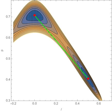
Figure 1: The contour plot of the potential $V_{{\rm gluon},4}(L,T)/b_{4}T$ at $\tilde{a}_{c}=a/T_{c}=2.237527$. The green linear line links the two degenerated vacua (31) and (32) shown by the red points. The shape of the potential as a function of $\ell$ or $p$ on the linear line corresponds to the black solid-line in Fig. 2.

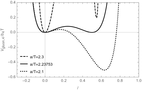
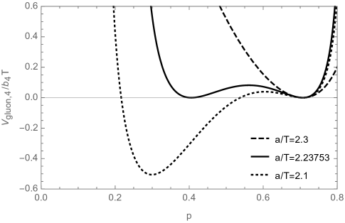
Figure 2: The potential $V_{{\rm gluon},4}(L,T)/b_{4}T$ as a function of $\ell$ (left) and of $p$ (right) on the straight line linking the two minimum points given in (31) and (32) around the critical temperature $\tilde{a}_{c}=a/T_{c}=2.237527$. Note that along the line $\ell$ increases while $p$ decreases.

There are two independent angles for $N=4$, and the traced Polyakov loop $\ell$ assumes the form

$$\ell =\frac{1}{2}\left(x_{1}+x_{2}\right),$$ (27)

where $x_{1}=\cos\theta_{1}$ and $x_{2}=\cos\theta_{2}$, and $V_{{\rm gluon},4}^{0}(L)$ is given by

$$V_{{\rm gluon},4}^{0}(L) =-\ln\left[(x_{1}-x_{2})^{4}(1-x_{1}^{2})(1-x_{2}^{2})\right]$$ (28)

up to a constant. Note that $V_{\rm gluon}^{0}(L)$ has no longer $Z_{N}$ center symmetry due to the reality assumption on $\ell$. Instead, $V_{{\rm gluon},4}^{0}(L)$ is invariant under $S_{2}\times Z_{2}$, under which $x_{1}$ and $x_{2}$ transform as

$$S_{2} :x_{1},x_{2}\to x_{2},x_{1}, Z_{2} :~{}x_{1},x_{2}\to-x_{2},-x_{1}.$$ (29)

Since $\ell$ transforms as $\ell\to-\ell$ under $Z_{2}$, $\ell$ is an order parameter for $Z_{2}$. An order parameter for $S_{2}$ is $p=(x_{1}-x_{2})/2$. In terms of these order parameters $V_{{\rm gluon},4}^{0}(L)$ can be rewritten as

$$V_{{\rm gluon},4}^{0}(L) =-\ln\left[p^{4}\left(1+\ell^{2}(\ell^{2}-2)+p^{2}(p^{2}-2)-2\ell^{2}p^{2}\right)\right],$$ (30)

where we have suppressed the constant in (30). Note that $|\ell|,|p|\leq 1$, and one finds that the absolute minimum of (30) in this interval is located at

$$\ell =0, p =\cos(\pi/4)=0.7071\dots$$ (31)

The two points $p=+\cos(\pi/4)$ and $p=-\cos(\pi/4)$ are the physically same point because of the permutation symmetry $S_{2}$ for $x_{1}$ and $x_{2}$ (and hence for $\theta_{1}$ and $\theta_{2}$). Consequently, $Z_{2}$ is unbroken, while $S_{2}$ is spontaneously broken.

In the presence of the kinetic term (the first term on the rhs of (22)) the location of the absolute minimum changes. We find that the critical value of $a/T$ denoted by $\tilde{a}_{c}$ is $2.237527$, and at $\tilde{a}_{c}$ the total potential $V_{{\rm gluon},4}(L,T)$ is minimized at two points in the $\ell-p$ plane (up to the sign of $\ell$ and $p$ because of the permutation symmetry $S_{2}$): The one is given in (31), and the second point is located at

$$\ell =0.4995, p =0.4056,$$ (32)

implying that $Z_{2}$ and $S_{2}$ are both spontaneously broken for $a/T<2.237527$. In Fig. 1 we show the contour plot of the potential $V_{{\rm gluon},4}(L,T)$ at $a/T=\tilde{a}_{c}=2.237527$ as a function of $\ell$ and of $p$. The green straight-line links the two minimum points (red points). Fig. 2 shows the shapes of the potential as a function of $\ell$ (left) or $p$ (right) on the straight line linking the two minimum points around $\tilde{a}_{c}$. The black solid-line corresponds to the green line in Fig.1.

$N=5$

In this case there are also two independent angles, and the traced Polyakov loop $\ell$ assumes the form

$$\ell =\frac{2}{5}\left(x_{1}+x_{2}+\frac{1}{2}\right),$$ (33)

where $x_{1}=\cos\theta_{1}$ and $x_{2}=\cos\theta_{2}$ (as in the case for $N=4$), and $V_{{\rm gluon},5}^{0}(L)$ is given by

$$V_{{\rm gluon},5}^{0}(L) =-\ln\left[(x_{1}-x_{2})^{4}(1-x_{1}^{2})(1-x_{2}^{2})(1-x_{1})^{2}(1-x_{2})^{2}\right]$$ (34)

up to a constant. Note that $V_{{\rm gluon},5}^{0}(L)$ has no longer $Z_{2}$ symmetry (29), but only the permutation symmetry $S_{2}$ for $x_{1}$ and $x_{2}$. Therefore, $\ell$ can no longer serve as an order parameter, while $p=(x_{1}-x_{2})/2$ is still a good order parameter for $S_{2}$.

Note that $|x_{1}|,|x_{2}|\leq 1$, and one finds that the absolute minimum in this interval appears at

$$x_{1} =\cos(2\pi/5)=0.30901\dots, x_{2} =\cos(4\pi/5)=-0.80901\dots,$$ (35)

(up to the permutation of $x_{1}$ and $x_{2}$), at which $\ell$ and $p$ take the value

$$\ell =0, p =\frac{\sqrt{5}}{4}=0.55901\dots$$ (36)

(up to the sign of $p$). So, $S_{2}$ is spontaneously broken as in the case for $N=4$. Although $\ell$ for $N=5$ is not related to any symmetry, the absolute minimum of $V_{{\rm gluon},5}^{0}(L)$ appears at $\ell=0$.

The presence of the kinetic term in (22) can change the location of the absolute minimum. We find that the transition is a first-order phase transition, and that the critical value of $a/T$ is $\tilde{a}_{c}=2.12699$. At $\tilde{a}_{c}$ the total potential $V_{{\rm gluon},5}(L,T)$ is minimized at two points in the $x_{1}-x_{2}$ plane (up to the the permutation of $x_{1}$ and $x_{2}$): The one is given in (36), and the second point is located at

$$x_{1} =0.7752, x_{2} =0.02621,$$ (37)

which means

$$\ell =0.5206, p =0.3745.$$ (38)

In Fig. 3 we plot the potential $V_{{\rm gluon},5}(L,T)$ at $a/T=\tilde{a}_{c}=2.12699$ on the $\ell$–$p$ plane. The two degenerated vacua (36) and (38) shown by the red points are linked by the green straight line. In Fig. 4, we show the shapes of the potential as a function of $\ell$ (left) or $p$ (right) on the straight line around the critical temperature.

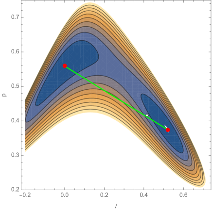
Figure 3: The contour plot of the potential $V_{{\rm gluon},5}(L,T)/b_{5}T$ at $\tilde{a}_{c}=a/T_{c}=2.12699$. The green linear line links the two degenerated vacua (31) and (32) shown by the red points. The shape of the potential as a function of $\ell$ or $p$ on the linear line corresponds to the black solid-line in Fig. 4.

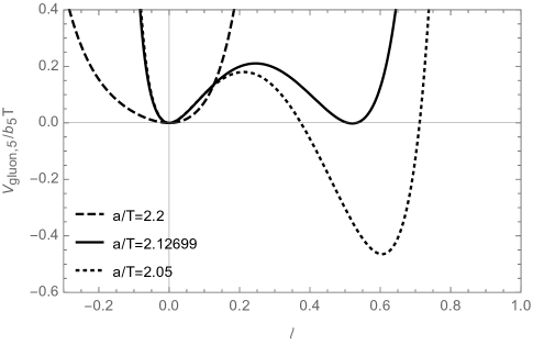
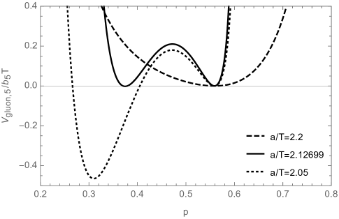
Figure 4: The potential $V_{{\rm gluon},5}(L,T)/b_{5}T$ as a function of $\ell$ (left) and of $p$ (right) on the straight line linking the two minimum points given in (36) and (38) around the critical temperature $\tilde{a}_{c}=a/T_{c}=2.12699$.

$N=6$

There are three independent angles for $N=6$, and the traced Polyakov loop $\ell$ is

$$\ell =\frac{1}{3}\left(x_{1}+x_{2}+x_{3}\right),$$ (39)

where $x_{i}=\cos\theta_{i}~{}(i=1,2,3)$, and $V_{{\rm gluon},6}^{0}(L)$ is given by

$$V_{{\rm gluon},6}^{0}(L) =-\ln\left[(x_{1}-x_{2})^{4}(x_{2}-x_{3})^{4}(x_{3}-x_{1})^{4}(1-x_{1}^{2})(1-x_{2}^{2})(1-x_{3}^{2})\right]$$ (40)

up to a constant. $V_{{\rm gluon},6}^{0}(L)$ is invariant under $S_{3}\times Z_{2}$, where $S_{3}$ consists of all the permutations of $x_{1},x_{2},x_{3}$, and $x_{1},x_{2},x_{3}\to-x_{2},-x_{1},-x_{3}$ under $Z_{2}$. $x_{1}$, $x_{2}$ and $x_{3}$ form a three dimensional reducible representation of $S_{3}$ and can be decomposed into the irreducible representations ${\bf 1}$ and ${\bf 2}$:

$${\bf 1}:~{}\ell=\frac{1}{3}\left(x_{1}+x_{2}+x_{3}\right), {\bf 2}:~{}\left(x_{1}-x_{2}~{},~{}(x_{1}+x_{2}-2x_{3})/\sqrt{3}\right).$$ (41)

The two dimensional representation can be further transformed to a complex representation

$$z =(x_{1}-x_{2})+i(x_{1}+x_{2}-2x_{3})/\sqrt{3}.$$ (42)

Then using $\ell$ and $z$ we can now express the potential as

$$V_{{\rm gluon},6}^{0}(L) =-\ln\left((z^{3}+z^{*3})^{4}\left[1-3\ell+3\ell^{2}-\ell^{3}-zz^{*}(1-\ell)/4+\frac{i}{24\sqrt{6}}(z^{3}-z^{*3})\right]\right.$$

$$\qquad\left.\times\left[1+3\ell+3\ell^{2}+\ell^{3}-zz^{*}(1+\ell)/4-\frac{i}{24\sqrt{6}}(z^{3}-z^{*3})\right]\right)$$ (43)

(up to a constant), which is invariant under $Z_{2}$:

$$\ell \to-\ell, z \to z^{*},$$ (44)

and under $Z_{3}$:

$$z \to\exp(2\pi ik/3)z, \ell \to\ell$$ (45)

with $k=1,2,3$. Since $\ell$ transforms as $\ell\to-\ell$ under $Z_{2}$, $\ell$ is an order parameter for $Z_{2}$, and the order parameter for $Z_{3}$ is $z$. We find that the absolute minimum under $|\ell|\leq 1$ and $|z|\leq 4/\sqrt{3}$ is located at

$$\ell =0, z =z^{*}=\sqrt{3}.$$ (46)

Therefore, $Z_{2}$ is unbroken, while $Z_{3}$ is spontaneously broken. Note that this vacuum corresponds to

$$x_{1} =\cos\!\left(\pi/6\right)=0.8660, x_{2} =\cos\!\left(5\pi/6\right)=-0.8660, x_{3} =\cos\!\left(3\pi/6\right)=0.$$ (47)

Now we include the kinetic term and find that the transition in this case is also a first-order phase transition. The critical value $\tilde{a}_{c}$ is $2.06064$, and the second minimum point at $a/T=\tilde{a}_{c}$ is located at

$$\ell =0.5299, z =0.99689-0.224514i, z^{*} =0.99689+0.224514i,$$ (48)

or equivalently,

$$x_{1} =0.9635, x_{2} =-0.03339, x_{3} =0.6595,$$ (49)

implying that $Z_{2}$ and $Z_{3}$ are both spontaneously broken for $a/T<2.06064$. In Fig. 5 we plot the potential $V_{{\rm gluon},6}(L,T)$ at $a/T=\tilde{a}_{c}=2.06064$ as a function of $\ell$ (upper panel) and $|z|$ (lower panel) varying along the three different lines $c_{1}~{}\mbox{(black)},c_{2}~{}\mbox{(red)}$ and $c_{3}~{}\mbox{(blue)}$, which link the two minimum points using a parameter $t$:

$$c_{1}: x_{1} =0.0975t+0.8660, x_{2} =0.83261t-0.8660, x_{3} =0.6595t$$ (50)

$$c_{2}: x_{1} =0.0975t^{2}+0.8660, x_{2} =0.83261t-0.8660, x_{3} =0.6595t^{3}$$ (51)

$$c_{3}: x_{1} =0.0975t+0.8660, x_{2} =0.83261t-0.8660, x_{3} =0.6595t^{2}.$$ (52)

We have (48) for $t=0$, while $t=1$ yields (49). In Fig. 6, we show the temperature evolution of the potential around the critical temperature for the three different lines $c_{1}$, $c_{2}$ and $c_{3}$.

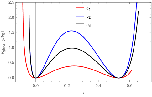
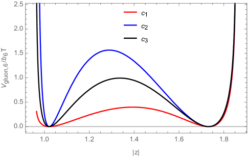
Figure 5: The potential $V_{{\rm gluon},6}(L,T)/b_{6}T$ at $\tilde{a}_{c}=2.06064$ as a function of $\ell$ (left) and $|z|$ (right) on the three different lines $c_{1}$ (red), $c_{2}$ (blue), $c_{3}$ (black) linking the two minimum points given in (46) and (48).

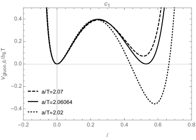
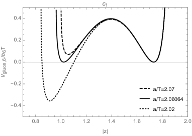
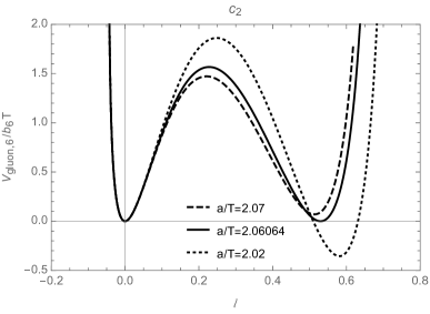
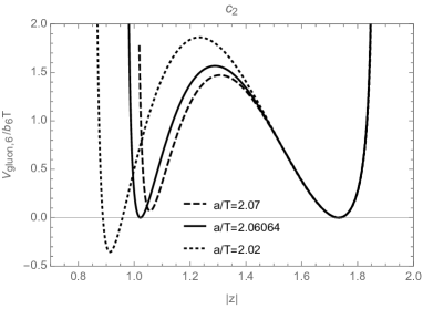
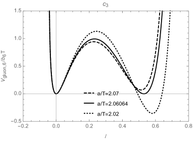
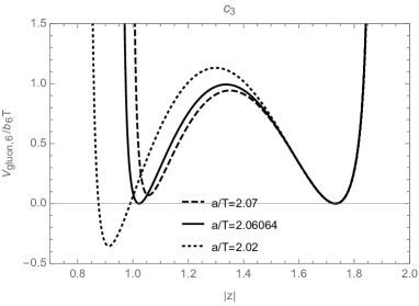
Figure 6: The potential $V_{{\rm gluon},6}(L,T)/b_{6}T$ around the critical temperature $\tilde{a}_{c}=2.06064$ as a function of $\ell$ (left) and $|z|$ (right) on the three different lines $c_{1}$, $c_{2}$, $c_{3}$ linking the two minimum points given in (46) and (48).

III.2.2 Scale phase transition

After we have analyzed the pure gluonic part $V_{\text{gluon}}\!\left(L,T\right)$, we here study the scale phase transition including the Polyakov loop effect. The matter part is $V_{\text{matter}}\!\left(L,f,T\right)=V_{\text{MFA}}\!\left(f\right)+V_{\rm FT}(L,f,T)$, where

$$V_{\text{MFA}}\!\left(f\right) =-N_{f}(N_{f}\lambda_{S}+\lambda_{S}^{\prime})f^{2}+\frac{NN_{f}}{32\pi^{2}}M^{4}\ln\frac{M^{2}}{\Lambda_{H}^{2}},$$ (53)

$$V_{\rm FT}(L,f,T) =2N_{f}T\int\frac{d^{3}p}{(2\pi)^{3}}\,{\rm Tr}\,\ln\!\left(1-L\,e^{-E_{p}/T}\right),$$ (54)

and $E_{p}=\sqrt{\vec{p}^{2}+\tilde{M}^{2}\!\left(T\right)}$ with the thermally dressed mass of $S$,

$$\tilde{M}^{2}\!\left(T\right) =\tilde{M}^{2}+\frac{T^{2}}{6}\Big{(}(NN_{f}+1)\lambda_{S}+(N_{f}+N)\lambda^{\prime}_{S}\Big{)}.$$ (55)

Here, $V_{\text{MFA}}$ is given in (53) with $S$ suppressed, and $\tilde{M}^{2}$ is defined in (7). ${\rm Tr}\,_{c}$ in (54) stands for the trace in the $SU(N)$ color space. Since the Polyakov loop is diagonal in the Polyakov gauge (14) and we assume that the angles $\theta$s are constants, the thermal effect part in (54) can be written as

$${\rm Tr}\,\ln\!\left(1-L\,e^{-E_{p}/T}\right)=\sum_{n=1}^{N}\ln\!\left(1-\exp\!\left(i\theta_{n}-E_{p}/T\right)\right).$$ (56)

Then using the reality condition (16), we find that

$$V_{\rm FT}(L,f,T) =-\frac{2N_{f}T^{2}{\tilde{M}}^{2}}{2\pi^{2}}\sum_{n=1}^{N}\sum_{j=1}^{\infty}\frac{e^{i(j\theta_{n})}}{j^{2}}K_{2}(j{\tilde{M}}/T)$$

$$=-\frac{2N_{f}T^{2}{\tilde{M}}^{2}}{\pi^{2}}\sum_{j=1}^{\infty}\frac{K_{2}(j{\tilde{M}}/T)}{j^{2}}$$

$$\quad\times\begin{cases}\left(\cos\!\left(j\theta_{1}\right)+\cdots+\cos\!\left(j\theta_{N/2}\right)\right)\\[10.0pt] \left(\cos\!\left(j\theta_{1}\right)+\cdots+\cos\!\left(j\theta_{(N-1)/2}\right)+1/2\right)\end{cases}~{}~{}\text{for}~{}~{}\begin{cases}\text{even}~{}~{}N\\[10.0pt] \text{odd }~{}~{}N\end{cases},$$ (57)

where $K_{2}\!\left(x\right)$ is the modified Bessel function of the second kind of order two, and we will truncate the sum at $j=10$. A useful identity is given by

$$\cos\!\left(j\theta_{i}\right)=T_{j}\!\left(x_{i}\right),$$ (58)

where $T_{n}\!\left(x\right)$ is the Chebyshev polynomials of the first kind which satisfies the recurrence relation, $T_{n+1}\!\left(x\right)=2xT_{n}\!\left(x\right)-T_{n-1}\!\left(x\right)$ with $T_{0}\!\left(x\right)=1$ and $T_{1}\!\left(x\right)=x$ for $n=1,2,\cdots$, and $x_{i}=\cos\theta_{i}$.

Since in the $N=3$ case the volume factor $b_{3}T$ approximately satisfies $b_{3}T\simeq T^{4}$ at the critical temperature Fukushima (2004), we assume that this relation holds for other $N$, too. Accordingly, we consider the dimensionless effective potential

$$V_{\text{eff}}\!\left(L,f,T\right)/T^{4}=V_{\text{matter}}\!\left(L,f,T\right)/T^{4}-6\exp\!\left(-a_{N}/T\right)N^{2}\ell+V^{0}_{\text{gluon},N}\!\left(L\right),$$ (59)

where the pure gluonic potential $V^{0}_{\text{gluon},N}\!\left(L\right)$ is given in (19). Further, since $f$ is a positive definite field with the canonical dimension two, we introduce a canonically defined field $\chi$ with the canonical dimension one:

$$f=\chi^{2}.$$ (60)

Note that the effective potential $V_{\text{eff}}\!\left(L,f=\chi^{2},T\right)$ is invariant under $\chi\to-\chi$.

For a given set of $\lambda_{S}$, $\lambda_{S}^{\prime}$, $N_{f}$ and $N$, the effective potential $V_{\text{eff}}\!\left(L,\chi,T\right)/T^{4}$ is controlled by $T$ and $a_{N}$. For an arbitrary choice of $T$ and $a_{N}$, the deconfinement and the scale transitions do not occur at the same temperature. Since we assume that the both transitions occur at the same temperature $T_{c,N}$, we have to adjust $T$ and $a_{N}$, such that this happens. We find that $T_{c,N}$ is not unique for a given set of $\lambda_{S}$ and $\lambda_{S}^{\prime}$, $N_{f}$ and $N$ and varies slightly as $a_{N}$ varies. In the following we consider the cases with $N=3,4,5$ and $6$ for the set of the other parameters given by

$$\lambda_{S} =1, \lambda_{S}^{\prime} =2, N_{f} =2.$$ (61)

$N=3$

To show behaviors of the effective potential, we here use (61) and the choice

$$T_{c,4}/\Lambda_{H} =14.38, a_{4}/\Lambda_{H} =40,$$ (62)

which yield the degenerated vacua

$$\text{(i) broken phase}: \chi/\Lambda_{H}=6.44464, \ell=0.22473,$$ (63)

$$(x_{1}=-0.16291)$$

$$\text{(ii) symmetric phase}: \chi/\Lambda_{H}=0, \ell=0.31247,$$ (64)

$$(x_{1}=-0.03129).$$

In order to plot the effective potential, let us define two lines linking the vacua (63) and (64):

$$c_{1}^{\prime}: \chi=6.4446t, x_{1}=-0.13162t-0.03129.$$ (65)

The effective potential along these lines is shown in Fig. 8. Fig. 8 shows the effective potential around the critical temperature (62).

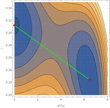
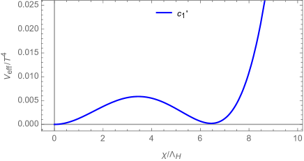
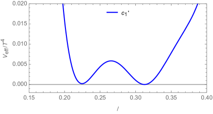
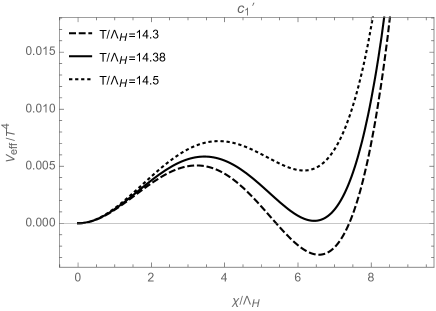
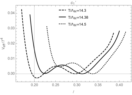
Figure 7: The potential $V_{\text{eff}}(L,\chi,T)/T^{4}$ at $T_{c,3}/\Lambda_{H}=14.38$ as a function of $\chi$ and $\ell$. The top panel is a contour plot on $\chi$–$\ell$ plane. The green line ($c_{1}^{\prime}$) links the degenerated vacua (63) and (64) which are shown by the red points. The bottom panels show the effective potential along the line $c_{1}^{\prime}$ as a function of $\chi$ (left) and $\ell$ (right).

Figure 8: The potential $V_{\text{eff}}(L,\chi,T)/T^{4}$ around $T_{c,3}/\Lambda_{H}=14.38$ as a function of $\chi$ (left) and $\ell$ (right) on the line $c_{1}^{\prime}$ linking the two minimum points given in (63) and (64).

$N=4$

As an example, we use (61) and the choice

$$T_{c,4}/\Lambda_{H} =6.670, a_{4}/\Lambda_{H} =16.$$ (66)

This set yields the following vacua:

$$\text{(i) broken phase}: \chi/\Lambda_{H}=2.9857, \ell=0.1510, p=0.6594,$$ (67)

$$(x_{1}=0.810, x_{2}=-0.5084)$$

$$\text{(ii) symmetric phase}: \chi/\Lambda_{H}=0, \ell=0.3723, p=0.5059,$$ (68)

$$(x_{1}=0.8781, x_{2}=-0.1336).$$

In order to plot the effective potential, let us define two lines linking the vacua (67) and (68):

$$c_{1}^{\prime}: \chi=2.9857t, x_{1}=-0.06775t+0.8781, x_{2}=-0.3748t-0.1336,$$ (69)

$$c_{2}^{\prime}: \chi=2.9857t, x_{1}=-0.06775t^{2}+0.8781, x_{2}=-0.3748t-0.1336.$$ (70)

The effective potential along these lines is shown in Fig. 10. In Fig. 10 we plot the effective potential around the critical temperature (66).

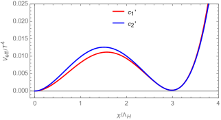
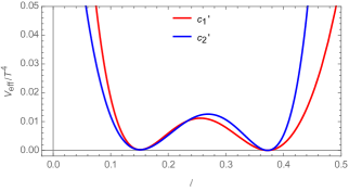
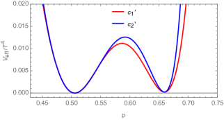
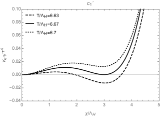
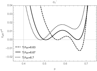
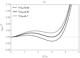
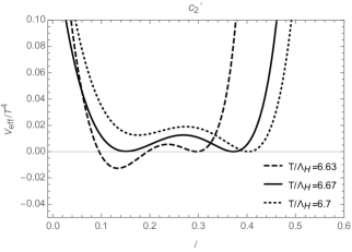
Figure 9: The potential $V_{\text{eff}}(L,\chi,T)/T^{4}$ at $T_{c,4}/\Lambda_{H}=6.670$ as a function of $\chi$ (left), $\ell$ (center) and $p$ (right) on the two different lines $c_{1}^{\prime}$ (red) and $c_{2}^{\prime}$ (blue) linking the two minimum points given in (67) and (68).

Figure 10: The potential $V_{\text{eff}}(L,\chi,T)/T^{4}$ around $T_{c,4}/\Lambda_{H}=6.670$ as a function of $\chi$ (left), $\ell$ (center) and $p$ (right) on the two different lines $c_{1}^{\prime}$ and $c_{2}^{\prime}$ linking the two minimum points given in (67) and (68).

$N=5$

With the parameter set (61) and the following choice

$$T_{c,5}/\Lambda_{H} =3.615, a_{5}/\Lambda_{H} =8.0,$$ (71)

we obtain

$$\text{(i) broken phase}: \chi/\Lambda_{H}=1.9088, \ell=0.1171, p=0.5938,$$ (72)

$$(x_{1}=0.4902, x_{2}=-0.6974)$$

$$\text{(ii) symmetric phase}: \chi/\Lambda_{H}=0, \ell=0.4733, p=0.4101,$$ (73)

$$(x_{1}=0.7517, x_{2}=-0.0684).$$

We make two lines connecting the vacua (72) and (73) as

$$c_{1}^{\prime}: \chi=1.9088t, x_{1}=-0.2615t+0.7517, x_{2}=-0.6290t-0.06840,$$ (74)

$$c_{2}^{\prime}: \chi=1.9088t, x_{1}=-0.2615t^{2}+0.7517, x_{2}=-0.6290t-0.06840.$$ (75)

The effective potential along these lines is shown in Fig. 12. In Fig. 12 we plot the effective potential around the critical temperature (71).

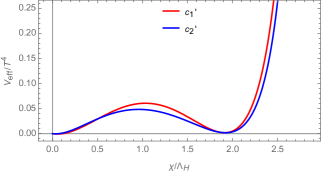
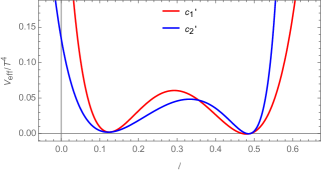
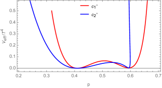
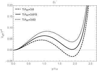
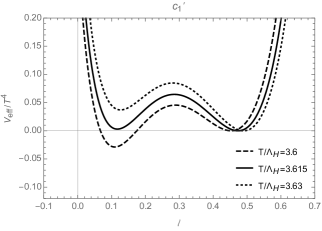
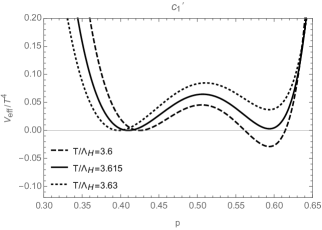
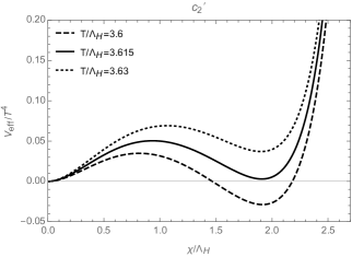
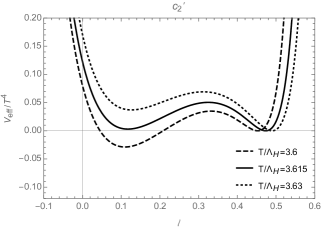
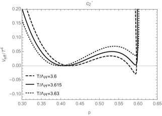
Figure 11: The potential $V_{\text{eff}}(L,\chi,T)/T^{4}$ at $T_{c,5}/\Lambda_{H}=3.615$ as a function of $\chi$ (left), $\ell$ (center) and $p$ (right) on the two different lines $c_{1}^{\prime}$ (red) and $c_{2}^{\prime}$ (blue) linking the two minimum points given in (72) and (73).

Figure 12: The potential $V_{\text{eff}}(L,\chi,T)/T^{4}$ around $T_{c,5}/\Lambda_{H}=3.615$ as a function of $\chi$ (left), $\ell$ (center) and $p$ (right) on the two different lines $c_{1}^{\prime}$ and $c_{2}^{\prime}$ linking the two minimum points given in (72) and (73).

$N=6$

A representative example of the critical value of $T$ and $a$ is

$$T_{c,6}/\Lambda_{H} =2.918, a_{6}/\Lambda_{H} =6.2.$$ (76)

At this critical point two minima of $V_{\text{eff}}\!\left(L,\chi,T\right)/T^{4}$ appear at:

$$\text{(i) broken phase}: \chi/\Lambda_{H}=1.3649, \ell=0.1107, z=1.0009-1.3806i, z^{*}=1.0009+1.3806i,$$ (77)

$$(x_{1}=0.2126, x_{2}=-0.78828, x_{3}=0.90782)$$

$$\text{(ii) symmetric phase}: \chi/\Lambda_{H}=0, \ell=0.48691, z=0.7528-0.81933i, z^{*}=0.7528+0.81933i,$$ (78)

$$(x_{1}=0.62679, x_{2}=-0.12601, x_{3}=0.95995).$$

We plot $V_{\text{eff}}\!\left(L,\chi,T\right)/T^{4}$ at the critical point (given in (76)) as a function of $\chi$ (left), $\ell$ (center) and $|z|$ in Fig. 14, where we vary $\chi$, $\ell$ and $|z|$ along the two different lines $c_{1}^{\prime}$ (red) and $c_{2}^{\prime}$ (black), which link the two minimum points:

$$c_{1}^{\prime}: \chi=1.3649t, x_{1}=-0.41419t+0.62679, x_{2}=-0.66227t-0.12601, x_{3}=-0.052131t+0.95995,$$ (79)

$$c_{2}^{\prime}: \chi=1.3649t, x_{1}=-0.41419t^{2}+0.62679, x_{2}=-0.66227t-0.12601, x_{3}=-0.052131t^{3}+0.95995.$$ (80)

Fig. 14 exhibits the effective potential around the critical temperature. From these figures we conclude that the scale phase transition for $N=6$ with the Polyakov loop effect included is a first-order phase transition.

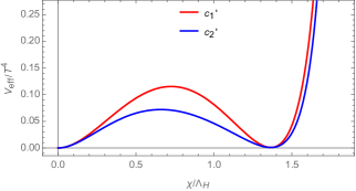
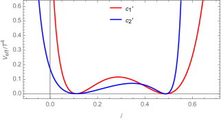
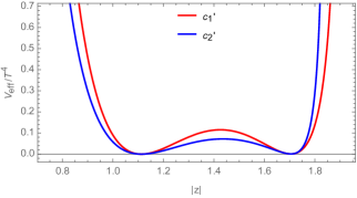
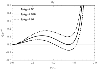
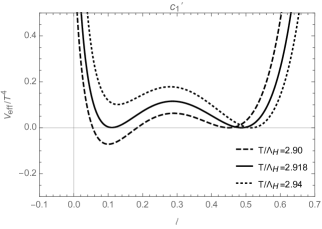
Figure 13: The potential $V_{\text{eff}}(L,\chi,T)/T^{4}$ at $T_{c,6}/\Lambda_{H}=2.918$ as a function of $\chi$ (left), $\ell$ (center) and $|z|$ (right) on the two different lines $c_{1}^{\prime}$ (red) and $c_{2}^{\prime}$ (blue) linking the two minimum points given in (77) and (78).

Figure 14: The potential $V_{\text{eff}}(L,\chi,T)/T^{4}$ around $T_{c,6}/\Lambda_{H}=2.918$ as a function of $\chi$ (left), $\ell$ (center) and $|z|$ (right) on the two different lines $c_{1}^{\prime}$ and $c_{2}^{\prime}$ linking the two minimum points given in (77) and (78).

III.2.3 Latent heat

Let us here evaluate the latent heat which is defined by

$$\epsilon\!\left(T\right)=-\Delta V_{\text{eff}}\!\left(L,\chi,T\right)+T\frac{\partial\Delta V_{\text{eff}}}{\partial T},$$ (81)

where $\Delta V_{\text{eff}}$ is the difference between those of broken phase (B.P.) and symmetric phase (S.P), namely, $\Delta V_{\text{eff}}\!\left(L,\chi,T\right)=V_{\text{eff}}\!\left(L,\chi,T\right)|_{\text{B.P.}}-V_{\text{eff}}\!\left(L,\chi,T\right)|_{\text{S.P.}}$. This is a key quantity of gravitational waves produced by a first-order phase transition. The larger the latent heat becomes, the stronger spectra of gravitational waves become.

We first evaluate the latent heat in the pure gluon case. Here, to this end, we set $a=1$ and $b_{N}=T^{3}$ in the effective potential of the Polyakov loop (22). In Table 1, we show the critical temperature and the latent heat normalized by $T_{c}^{4}$. We see that larger number of the color yields the larger latent heat, which can be understood from the analytic expression

$$\epsilon(T_{c})/T_{c}^{4}=\frac{b_{N}}{T_{c}^{4}}e^{-1/T_{c}}\ln\ell_{c}^{2}~{},$$ (82)

where $\ell_{c}$ is the traced Polyakov loop in the de-confining phase.

Table 1: Critical temperature and latent heat in pure gluon case with $a=1$ and $b_{N}=T^{3}$.

$N$	$T_{c}$	$\epsilon\!\left(T_{c}\right)/T_{c}^{4}$
3	0.40736	2.2857
4	0.44692	5.7278
5	0.47015	10.313
6	0.48529	15.917

Next, we consider the system where the scalar field is coupled with the Polyakov loop. Here, before evaluating the latent heat numerically, let us describe what we could observe when the Polyakov loop effects are taken into account. In the case without the Polyakov loop, the vacuum contribution from the scalar field loop at finite temperature is

$$V_{\rm FT}^{\text{wo}}(0,T) =-2N_{f}N\times\frac{\pi^{2}}{90}T^{4}.$$ (83)

Since this term does not depend on the field $\chi$ and is subtracted in $\Delta V_{\text{eff}}\!\left(\chi,T\right)$, it does not contribute to the latent heat (81). In contrast, when we take the Polyakov loop effects into account, as one can see from (57), the traced Polyakov loop is coupled to the vacuum contribution (83):

$$V_{\rm FT}^{\text{w}}(L,0,T) =-\frac{4N_{f}T^{4}}{\pi^{2}}\sum_{j=1}^{\infty}\frac{1}{j^{4}}\times\begin{cases}\left(\cos\!\left(j\theta_{1}\right)+\cdots+\cos\!\left(j\theta_{N/2}\right)\right)\\[10.0pt] \left(\cos\!\left(j\theta_{1}\right)+\cdots+\cos\!\left(j\theta_{(N-1)/2}\right)+1/2\right)\end{cases}~{}~{}\text{for}~{}~{}\begin{cases}\text{even}~{}~{}N\\[10.0pt] \text{odd }~{}~{}N\end{cases},$$ (84)

where we used the fact that $K_{2}\!\left(x\right)=2/x^{2}-1/2+\cdots$. Note that if we set all angles to zero ($\theta_{1}=\theta_{2}=\cdots=0$), (84) produces (83) using $\sum_{j=1}^{\infty}\frac{1}{j^{4}}=\zeta\!\left(4\right)=\pi^{4}/90$. Then, we see the relation between the vacuum contributions with and without the Polyakov loop:

$$V_{\rm FT}^{\text{w}}(L,0,T)=V_{\rm FT}^{\text{wo}}(0,T)\times\frac{90}{\pi^{4}}\sum_{j=1}^{\infty}\frac{1}{j^{4}}\Upsilon\!\left(j,\{\theta_{i}\}\right),$$ (85)

where

$$\Upsilon\!\left(j,\{\theta_{i}\}\right)=\frac{2}{N}\begin{cases}\left(\cos\!\left(j\theta_{1}\right)+\cdots+\cos\!\left(j\theta_{N/2}\right)\right)\\[10.0pt] \left(\cos\!\left(j\theta_{1}\right)+\cdots+\cos\!\left(j\theta_{(N-1)/2}\right)+1/2\right)\end{cases}~{}~{}\text{for}~{}~{}\begin{cases}\text{even}~{}~{}N\\[10.0pt] \text{odd }~{}~{}N\end{cases}.$$ (86)

Note that $\Upsilon\!\left(j=1,\{\theta_{i}\}\right)=\ell$. Since $\Upsilon\!\left(j,\{\theta_{i}\}\right)$ takes different values between broken and symmetric phases, the vacuum term (85) contributes to the latent heat.

We show the $N=6$ case with the parameters (61) and (76). Fig. 15 shows the latent heat normalized by $T^{4}$ slightly below the critical temperature. At the critical temperature, we have vacua (77) and (78) at which the latent heat in the case with and without the Polyakov loop is

$$\frac{\epsilon\!\left(T_{c}\right)}{T_{c}^{4}}=\begin{cases}10.3733&\text{with Polyakov loop}\\[10.0pt] 1.02791&\text{without Polyakov loop}\end{cases}.$$ (87)

We see that the Polyakov loop effect increases the latent heat. The vacuum contribution (85) at the critical temperature becomes $\Delta\epsilon\!\left(T_{c}^{4}\right)/T_{c}^{4}=2.4905$. That is, this contribution accounts for about $24\%$ within the total contribution (87). In Fig. 15, we show the temperature-dependence of the latent heat slightly below the critical temperature. We see that there is a jump at about $T/T_{c}=0.99724$. Below this temperature, the scalar condensate takes different values between the true and false vacua, whereas the Polyakov loop does not. In other words, the false vacuum for the Polyakov loop in the effective potential appears above $T/T_{c}=0.99724$. Once the false vacuum of the Polyakov loop is generated, the latent heat could be large.

Figure 15: The latent heat (81) normalized by $T^{4}$ as a function of $T/T_{c}$.

IV Summary

In this paper we have considered scalegenesis, the spontaneous breaking of scale invariance, by the condensation of the scalar bilinear in an $SU(N)$ gauge theory, where the scalar field is in the fundamental representation of $SU(N)$. This non-perturbative effect has been studied by means of an effective theory which we have developed in Kubo and Yamada (2016a, 2015, b); Kubo et al. (2018). In the previous formulation of the effective theory no confinement effect has been taken into account. Following the ansatz of Fukushima (2004) we have included the Polyakov loop effect into the scale phase transition at finite temperature, where we have assumed that the deconfinement transition and the scale phase transition appear at the same critical temperature. $N$ is not restricted to $3$ in phenomenological applications of the scalar-bilinear condensation in a scale invariant extension of the SM. We therefore have studied the cases with $N=3,4,5$ and $6$ and found that in all these cases the phase transition is a first-order phase transition. We could introduce a current scalar mass (which breaks the scale symmetry softly and investigate the change of the nature of the scale phase transition. As in QCD we expect the scale phase transition will become cross-over type above some current scalar mass. But this would go beyond the scope of our paper, and we would like to leave it to the next project.

Since the latent heat is an important quantity to estimate the strength of the gravitational waves background which is produced by a first-order phase transition in the early Universe, we have calculated it at and slightly below the critical temperature and compared the results with those obtained without the Polyakov loop effect. We have found that the Polyakov effect can indeed increase the latent heat if the cosmological phase transition occurs very close to the critical temperature of the first-order phase transition. This would mean a large increase in the energy density of the gravitational waves background, if it were produced by the scale phase transition.

Acknowledgements

M. Y. thanks Jan. M. Pawlowski for valuable discussions. The work of J. K. is partially supported by the Grant-in-Aid for Scientific Research (C) from the Japan Society for Promotion of Science (Grant No.16K05315). The work of M. Y. is supported by the DFG Collaborative Research Centre SFB1225 (ISOQUANT).

References

- Gildener (1976) E. Gildener, Phys. Rev. D14, 1667 (1976).
- Weinberg (1979) S. Weinberg, Phys. Lett. B82, 387 (1979).
- Oda and Yamada (2016) K.-y. Oda and M. Yamada, Class. Quant. Grav. 33, 125011 (2016), eprint 1510.03734.
- Wetterich and Yamada (2017) C. Wetterich and M. Yamada, Phys. Lett. B770, 268 (2017), eprint 1612.03069.
- Hamada and Yamada (2017) Y. Hamada and M. Yamada, JHEP 08, 070 (2017), eprint 1703.09033.
- Eichhorn et al. (2018) A. Eichhorn, Y. Hamada, J. Lumma, and M. Yamada, Phys. Rev. D97, 086004 (2018), eprint 1712.00319.
- Niedermaier and Reuter (2006) M. Niedermaier and M. Reuter, Living Rev. Rel. 9, 5 (2006).
- Niedermaier (2007) M. Niedermaier, Class. Quant. Grav. 24, R171 (2007), eprint gr-qc/0610018.
- Percacci (2007) R. Percacci (2007), eprint 0709.3851.
- Reuter and Saueressig (2012) M. Reuter and F. Saueressig, New J. Phys. 14, 055022 (2012), eprint 1202.2274.
- Codello et al. (2009) A. Codello, R. Percacci, and C. Rahmede, Annals Phys. 324, 414 (2009), eprint 0805.2909.
- Eichhorn (2017) A. Eichhorn, in Black Holes, Gravitational Waves and Spacetime Singularities Rome, Italy, May 9-12, 2017 (2017), eprint 1709.03696, URL http://inspirehep.net/record/1623009/files/arXiv:1709.03696.pdf.
- Percacci (2017) R. Percacci, An Introduction to Covariant Quantum Gravity and Asymptotic Safety, vol. 3 of 100 Years of General Relativity (World Scientific, 2017), ISBN 9789813207172, 9789813207196, 9789813207172, 9789813207196.
- Wetterich (1984) C. Wetterich, Phys. Lett. B140, 215 (1984).
- Bardeen (1995) W. A. Bardeen, in Ontake Summer Institute on Particle Physics Ontake Mountain, Japan, August 27-September 2, 1995 (1995).
- Aoki and Iso (2012) H. Aoki and S. Iso, Phys. Rev. D86, 013001 (2012), eprint 1201.0857.
- Coleman and Weinberg (1973) S. R. Coleman and E. J. Weinberg, Phys. Rev. D7, 1888 (1973).
- Hur and Ko (2011) T. Hur and P. Ko, Phys. Rev. Lett. 106, 141802 (2011), eprint 1103.2571.
- Heikinheimo et al. (2014) M. Heikinheimo, A. Racioppi, M. Raidal, C. Spethmann, and K. Tuominen, Mod. Phys. Lett. A29, 1450077 (2014), eprint 1304.7006.
- Holthausen et al. (2013) M. Holthausen, J. Kubo, K. S. Lim, and M. Lindner, JHEP 12, 076 (2013), eprint 1310.4423.
- Kubo et al. (2014) J. Kubo, K. S. Lim, and M. Lindner, JHEP 09, 016 (2014), eprint 1405.1052.
- Heikinheimo and Spethmann (2014) M. Heikinheimo and C. Spethmann, JHEP 12, 084 (2014), eprint 1410.4842.
- Carone and Ramos (2015) C. D. Carone and R. Ramos, Phys. Lett. B746, 424 (2015), eprint 1505.04448.
- Ametani et al. (2015) Y. Ametani, M. Aoki, H. Goto, and J. Kubo, Phys. Rev. D91, 115007 (2015), eprint 1505.00128.
- Kubo and Yamada (2016a) J. Kubo and M. Yamada, Phys. Rev. D93, 075016 (2016a), eprint 1505.05971.
- Haba et al. (2016) N. Haba, H. Ishida, N. Kitazawa, and Y. Yamaguchi, Phys. Lett. B755, 439 (2016), eprint 1512.05061.
- Hatanaka et al. (2016) H. Hatanaka, D.-W. Jung, and P. Ko, JHEP 08, 094 (2016), eprint 1606.02969.
- Ishida et al. (2017) H. Ishida, S. Matsuzaki, S. Okawa, and Y. Omura, Phys. Rev. D95, 075033 (2017), eprint 1701.00598.
- Haba and Yamada (2017a) N. Haba and T. Yamada, Phys. Rev. D95, 115016 (2017a), eprint 1701.02146.
- Haba and Yamada (2017b) N. Haba and T. Yamada, Phys. Rev. D95, 115015 (2017b), eprint 1703.04235.
- Tsumura et al. (2017) K. Tsumura, M. Yamada, and Y. Yamaguchi, JCAP 1707, 044 (2017), eprint 1704.00219.
- Aoki et al. (2017) M. Aoki, H. Goto, and J. Kubo, Phys. Rev. D96, 075045 (2017), eprint 1709.07572.
- Osterwalder and Seiler (1978) K. Osterwalder and E. Seiler, Annals Phys. 110, 440 (1978).
- Fradkin and Shenker (1979) E. H. Fradkin and S. H. Shenker, Phys. Rev. D19, 3682 (1979).
- Nambu and Jona-Lasinio (1961a) Y. Nambu and G. Jona-Lasinio, Phys. Rev. 122, 345 (1961a).
- Nambu and Jona-Lasinio (1961b) Y. Nambu and G. Jona-Lasinio, Phys. Rev. 124, 246 (1961b).
- Kubo et al. (2018) J. Kubo, Q. M. B. Soesanto, and M. Yamada, Eur. Phys. J. C78, 218 (2018), eprint 1712.06324.
- Kubo and Yamada (2015) J. Kubo and M. Yamada, PTEP 2015, 093B01 (2015), eprint 1506.06460.
- Kubo and Yamada (2016b) J. Kubo and M. Yamada, JCAP 1612, 001 (2016b), eprint 1610.02241.
- Seto et al. (2001) N. Seto, S. Kawamura, and T. Nakamura, Phys. Rev. Lett. 87, 221103 (2001), eprint astro-ph/0108011.
- Kawamura et al. (2006) S. Kawamura et al., Class. Quant. Grav. 23, S125 (2006).
- Kawamura et al. (2011) S. Kawamura et al., Class. Quant. Grav. 28, 094011 (2011).
- Seoane et al. (2013) P. A. Seoane et al. (eLISA) (2013), eprint 1305.5720.
- Weiss (1981) N. Weiss, Phys. Rev. D24, 475 (1981).
- Pisarski (2000) R. D. Pisarski, Phys. Rev. D62, 111501 (2000), eprint hep-ph/0006205.
- Dumitru and Pisarski (2001) A. Dumitru and R. D. Pisarski, Phys. Lett. B504, 282 (2001), eprint hep-ph/0010083.
- Dumitru and Pisarski (2002) A. Dumitru and R. D. Pisarski, Phys. Lett. B525, 95 (2002), eprint hep-ph/0106176.
- Pisarski (2002) R. D. Pisarski, Nucl. Phys. A702, 151 (2002), eprint hep-ph/0112037.
- Sannino (2005) F. Sannino, Phys. Rev. D72, 125006 (2005), eprint hep-th/0507251.
- Marhauser and Pawlowski (2008) F. Marhauser and J. M. Pawlowski (2008), eprint 0812.1144.
- Braun et al. (2010) J. Braun, A. Eichhorn, H. Gies, and J. M. Pawlowski, Eur. Phys. J. C70, 689 (2010), eprint 1007.2619.
- Fukushima (2004) K. Fukushima, Phys. Lett. B591, 277 (2004), eprint hep-ph/0310121.
- Ratti et al. (2006) C. Ratti, M. A. Thaler, and W. Weise, Phys. Rev. D73, 014019 (2006), eprint hep-ph/0506234.
- Roessner et al. (2007) S. Roessner, C. Ratti, and W. Weise, Phys. Rev. D75, 034007 (2007), eprint hep-ph/0609281.
- Fukushima (2008) K. Fukushima, Phys. Rev. D77, 114028 (2008), [Erratum: Phys. Rev.D78,039902(2008)], eprint 0803.3318.
- Herbst et al. (2011) T. K. Herbst, J. M. Pawlowski, and B.-J. Schaefer, Phys. Lett. B696, 58 (2011), eprint 1008.0081.
- Fukushima and Hatsuda (2011) K. Fukushima and T. Hatsuda, Rept. Prog. Phys. 74, 014001 (2011), eprint 1005.4814.
- Fukushima and Sasaki (2013) K. Fukushima and C. Sasaki, Prog. Part. Nucl. Phys. 72, 99 (2013), eprint 1301.6377.
- Fukushima and Skokov (2017) K. Fukushima and V. Skokov, Prog. Part. Nucl. Phys. 96, 154 (2017), eprint 1705.00718.
- Bardeen et al. (1986) W. A. Bardeen, C. N. Leung, and S. T. Love, Phys. Rev. Lett. 56, 1230 (1986).
- Polyakov (1978) A. M. Polyakov, Phys. Lett. 72B, 477 (1978).
- Susskind (1979) L. Susskind, Phys. Rev. D20, 2610 (1979).
- Svetitsky and Yaffe (1982) B. Svetitsky and L. G. Yaffe, Nucl. Phys. B210, 423 (1982).
- Svetitsky (1986) B. Svetitsky, Phys. Rept. 132, 1 (1986).
- Greensite (2003) J. Greensite, Prog. Part. Nucl. Phys. 51, 1 (2003), eprint hep-lat/0301023.
- Fukugita and Ukawa (1986) M. Fukugita and A. Ukawa, Phys. Rev. Lett. 57, 503 (1986).
- Karsch and Laermann (1994) F. Karsch and E. Laermann, Phys. Rev. D50, 6954 (1994), eprint hep-lat/9406008.
- Aoki et al. (1998) S. Aoki et al. (JLQCD), Phys. Rev. D57, 3910 (1998), eprint hep-lat/9710048.
- Karsch et al. (2001) F. Karsch, E. Laermann, and A. Peikert, Nucl. Phys. B605, 579 (2001), eprint hep-lat/0012023.
- Allton et al. (2002) C. R. Allton, S. Ejiri, S. J. Hands, O. Kaczmarek, F. Karsch, E. Laermann, C. Schmidt, and L. Scorzato, Phys. Rev. D66, 074507 (2002), eprint hep-lat/0204010.
- Haas et al. (2013) L. M. Haas, R. Stiele, J. Braun, J. M. Pawlowski, and J. Schaffner-Bielich, Phys. Rev. D87, 076004 (2013), eprint 1302.1993.
- Kondo (2015) K.-I. Kondo (2015), eprint 1508.02656.
- Shirogane et al. (2016) M. Shirogane, S. Ejiri, R. Iwami, K. Kanaya, and M. Kitazawa, Phys. Rev. D94, 014506 (2016), eprint 1605.02997.