Nuclear systems under extreme conditions: isospin asymmetry and strong B-fields

Dissertation
zur Erlangung des Doktorgrades
der Naturwissenschaften

vorgelegt beim Fachbereich Physik
der Johann Wolfgang Goethe–Universität
in Frankfurt am Main

von
Martin Stein
aus Frankfurt am Main

Frankfurt am Main 2015
(D30)

vom Fachbereich Physik der Johann Wolfgang Goethe–Universität
in Frankfurt am Main als Dissertation angenommen

Dekan	Prof. Dr. Rene Reifarth
Gutachter	Prof. Dr. Joachim A. Maruhn, PD Dr. Armen Sedrakian
Datum der Disputation	16. Dezember 2015

Übersicht

Diese Doktorarbeit beschäftigt sich mit Kernmaterie und Atomkernen unter extremen Bedingungen, wie sie z.B. in kompakten Sternen vorkommen können. Kapitel 1 untersucht suprafluide Neutron-Proton Paarung in Isospin-asymmetrischer Kernmaterie im ${}^{3}S_{1}$-${}^{3}D_{1}$ Kanal. In Kapitel 2 untersuchen wir den Einfluß starker Magnetfelder auf [12]C, [16]O und [20]Ne. Abschließend untersuchen wir in Kapitel 3 suprafluide Neutron-Neutron Paarung in Spin-asymmetrischer (polarisierter) Neutronenmaterie im ${}^{1}S_{0}$ Kanal; eine Polarisation kann z.B. durch ein magnetisches Feld verursacht werden.

In Kapitel 1 erhalten wir ein reichhaltiges Phasendiagramm für Isospin-asymmetrische Kernmaterie. Ein besseres Verständnis dieser Materie kann z.B. für niederenergetische Schwerionenkollisionen, Supernovaexplosionen oder Atomkerne wichtig sein. Im äußeren Bereich von Atomen ist die Dichte gering. Dies führt dazu, dass eine Isospin-Asymmetrie die Neutron-Proton-Paarung kaum unterdrückt. Wir untersuchen die ungepaarte Phase und verschiedene suprafluide Phasen. Wir untersuchen den Crossover von der schwach gebundenen Bardeen Cooper Schrieffer (BCS) Phase bei hohen Dichten hin zum Bose-Einstein-Kondensat (englisch: Bose-Einstein condensate) (BEC) im Grenzfall starker Kopplung bei niedrigen Dichten. Außerdem untersuchen wir zwei exotische Phasen: Die Larkin-Ovchinnikov-Fulde-Ferrell (LOFF) Phase, bei der die Cooper-Paare einen endlichen Schwerpunktsimpuls erhalten. Diese Phase taucht nur bei hohen Dichten auf. Außerdem untersuchen wir eine Phasenseparation (PS), bei der die Materie in einen Isospin-symmetrischen Teil in der BCS oder BEC Phase und einen ungepaarten Teil mit Neutronenüberschuss aufgeteilt wird. Die Phasenseparation kann sowohl bei hohen als auch bei niedrigen Dichten auftauchen, weshalb wir in der Phasenseparation einen Crossover erhalten. Der Phasenübergang zwischen LOFF und PS ist erster Ordnung, alle anderen sind Phasenübergänge zweiter Ordnung. Außerdem untersuchen wir den Gap, den Kernel der Gap-Gleichung, die Wellenfunktionen der Cooper-Paare, die Besetzungszahlen und die Einteilchenenergien. Im BCS Grenzfall erhalten wir ein fermionisches und im BEC Grenzfall erhalten wir ein bosonisches Verhalten. Im Fall der LOFF Phase nähern sich die oben aufgeführten Funktionen denen der BCS Phase mit verschwindender Isospin-Asymmetrie an.

In Kapitel 2 untersuchen wir den Einfluss eines starken Magnetfeldes auf die Elemente [16]O, [12]C und [20]Ne. Diese Elemente können z.B. in Weißen Zwergen vorkommen, welche starke Magnetfelder aufweisen können. Des Weiteren können diese Elemente bei akkretierenden Neutronensternen eine Rolle spielen. Bei [16]O und [12]C werden die Einteilchenenergien mit zunehmendem Magnetfeld aufgespalten. Außerdem werden Bahndrehimpuls und Spin bei starken Magnetfeldern am Magnetfeld ausgerichtet, diese Ausrichtung wird bei schwachen Magnetfeldern durch die Spin-Bahn-Kopplung unterdrückt. Bei starken Magnetfeldern werden bei [16]O die Energieniveaus umbesetzt. Die kollektive Fließgeschwindigkeit in den Atomkernen beschreibt kreisförmige oder nahezu kreisförmige Bahnen um die Magnetfeldachse. Die Spindichte richtet sich bei starkem Magnetfeld aus. [20]Ne ist bei verschwindendem Magnetfeld stark verformt, diese Verformung nimmt mit zunehmendem Magnetfeld ab.

Das in Kapitel 3 untersuchte Phasendiagramm für polarisierte Neutronenmaterie kann für Studien in Neutronenmaterie von großer Bedeutung sein; besonders für die innere Kruste von Neutronensternen. Auch für Untersuchungen an Atomkernen kann es von Bedeutung sein. Es gibt phänomenologische Hinweise auf Neutronen-Suprafluidität in Neutronensternen. Das erhaltene Phasendiagramm besteht nur aus der ungepaarten Phase und der BCS Phase. Da es keine gebundenen Neutron-Neutron-Paare gibt, kann kein BEC entstehen. Da die Kopplungsstärke im ${}^{1}S_{0}$ Kanal schwächer ist als im ${}^{3}S_{1}$-${}^{3}D_{1}$ Kanal, ist die kritische Temperatur geringer als bei dem in Kapitel 1 analysierten Phasendiagramm. Für die mikroskopischen Funktionen erhalten wir ähnliche Resultate wie für die BCS Phase in Kapitel 1. Außerdem haben wir das für eine bestimmte Polarisation benötigte Magnetfeld berechnet und dessen Energie mit der Temperatur des Systems verglichen. Hierbei ist die magnetische Energie in dem von uns analysiertem Bereich in der Regel größer als die Temperatur.

Zusammenfassung

Einleitung

In dieser Arbeit untersuchen wir Kernmaterie und Atomkerne unter extremen Bedingungen. In Kapitel 1 und 3 untersuchen wir suprafluide Phasen von Kernmaterie bzw. Neutronenmaterie. In Kapitel 2 und 3 untersuchen wir den Einfluss starker Magnetfelder auf Atomkerne bzw. auf Neutronenmaterie.

Die Untersuchungen der Crossovers mit Einbeziehung von unkonventionellen Phasen, wie sie in Kapitel 1 erörtert werden, könnte hilfreich sein bei Untersuchungen von fermionischen Systemen mit unausgeglichenem Spin/Flavor in ultrakalten atomischen Gasen, siehe z.B. [1, 2, 3], farbsupraleitender dichter Quarkmaterie, siehe z.B. [4, 5, 6, 7, 8], oder anderen verwandten Quantensystemen. Bei niederenergetischen Schwerionenkollisionen erhält man im Endzustand viele Deuteronen, welche ${}^{3}S_{1}$-${}^{3}D_{1}$ Kondensation nahelegen [9]. Große Atomkerne wie z.B. ⁹²Pd könnten Neutron-Proton-Paare aufweisen [10].

Neutron-Neutron-Paarung wird z.B. in [11, 12, 13, 14, 15, 16, 17] untersucht. Neutron-Neutron-Paarung kann wichtig für Studien von Neutronensternmaterie sein, besonders für die innere Kruste, und für Atomkerne, besonders für neutronenreiche wie z.B. ¹¹Li, welches einen Neutron-Halo besitzt [13]. Die Rotation von Neutronensternen und Anomalien in der Rotation sprechen für suprafluide Phasen [17].

Neutron-Proton-Paarung kann eine wichtige Rolle in Supernova-Materie spielen, in der die Isospin-Asymmetrie gering ist. Sie kann auch im äußeren Bereich von Atomkernen auftreten; aufgrund der geringen Dichte unterdrückt die dort vorherrschende Isospin-Asymmetrie die Neutron-Proton-Paarung kaum.

Suprafluide Materie

Bei hohen Dichten von $\rho\lesssim\frac{1}{2}\rho_{0}$ mit $\rho_{0}=0{,}16\,$fm^-3, was $2{,}8\cdot 10^{14}\,$g cm^-3 entspricht, können verschiedene suprafluide Phasen auftreten; hierbei steht $\rho_{0}$ für die Kernsättigungsdichte. Diese Phasen sind mathematisch der Phase supraleitender Elektronen sehr ähnlich. Ähnlich wie bei Supraleitung muss auch bei Suprafluidität die Temperatur gering sein, wobei die Temperatur hierbei gering bezüglich der anderen relevanten Energien sein muss. Tiefe Temperatur bedeutet in diesem Zusammenhang bis zu mehrere MeV, wobei ein MeV einer Temperatur von $11{,}6\cdot 10^{9}$ K entspricht.

Bei ausreichend hohen Dichten erreichen die chemischen Potenziale der Nukleonen Werte, die mit der Ruhemasse von Hyperonen vergleichbar sind. In diesem Fall kann die Materie mit Hyperonen angereichert werden, dies kann bei doppelter Kernsättigungsdichte geschehen. Wenn die Dichten sehr groß werden, wird der Teilchenabstand kleiner als der Nukleonenradius und das Confinement kann aufgehoben werden.

Supraleitende bzw. suprafluide Paarung kann zwischen ähnlichen Fermionen auftreten, die sich aufgrund des Pauli Prinzips in mindestens einer Quantenzahl unterscheiden müssen. So kann z.B. eine supraleitende bzw. suprafluide Paarung von zwei Elektronen, Neutronen oder Protonen unterschiedlichen Spins entstehen. Zwei Nukleonen unterschiedlichen Isospins, also ein Proton und ein Neutron, können auch mit gleichem Spin eine suprafluide Paarung eingehen. Da der Massenunterschied zwischen Neutronen und Protonen weniger als 0,14% der Nukleonenmasse beträgt, können die Effekte, die aufgrund des Massenunterschiedes auftreten, vernachlässigt werden. Die Ruhemasse eines Neutrons beträgt 939,6 MeV und die eines Protons beträgt 938,3 MeV.

Aus der Streutheorie von Nukleonen kann man die kritische Temperatur verschiedener Paarungskanäle berechnen [17]. Bei den für uns interessanten Dichten ist der Spin-Triplett ${}^{3}S_{1}$-${}^{3}D_{1}$ Kanal dominant, wobei er für Isospin-Triplett-Paarung (Neutron-Neutron-Paarung) aufgrund des Pauli-Prinzips verboten ist. Der für Isospin-Triplett-Paarung dominante Kanal ist der deutlich schwächere Isospin-Singulett ${}^{1}S_{0}$ Kanal.

In Kapitel 1 untersuchen wir Isospin-Singulett Spin-Triplett Paarung (Neutron-Proton-Paarung mit gleichem Spin) im ${}^{3}S_{1}$-${}^{3}D_{1}$ Kanal in Kernmaterie und in Kapitel 3 untersuchen wir Isospin-Triplett Spin-Singulett Paarung (Neutron-Neutron-Paarung mit unterschiedlichem Spin) im ${}^{1}S_{0}$ Kanal in Neutronenmaterie. In Isospin-symmetrischer Kernmaterie bzw. Spin-symmetrischer Neutronenmaterie haben wir für tiefe Temperaturen Paarung in der Bardeen Cooper Schrieffer (BCS) Phase. Hierbei findet eine Paarung zwischen zwei Nukleonen statt, deren Impuls betragsmäßig gleich ist, deren Richtung aber entgegengesetzt ist (${\bm{k}}_{1}=-{\bm{k}}_{2}$). Günstig für eine Paarung sind sowohl eine hohe Zustandsdichte als auch eine hohe Kopplungsstärke. Die Zustandsdichte nimmt mit steigender Dichte zu, die Kopplungsstärke dagegen nimmt ab. Die Zustandsdichte dominiert für geringe und die Kopplungsstärke für hohe Dichten. Für den Gap bei verschwindender Temperatur und Asymmetrie $\Delta_{00}$ finden wir folgende Relation:

$$\Delta_{00} = 2\varepsilon_{F}\cdot e^{-\frac{1}{NV}}\,.$$ (1)

Folglich steigt der Gap für geringe Dichten mit zunehmender Dichte, wohingegen er bei hohen Dichten abfällt. Die kritische Temperatur $T_{C}$ ist proportional zu diesem Gap:

$$\Delta_{00}=1{,}76\,T_{C}\,.$$ (2)

Die Asymmetrie $\alpha$ bezieht sich im Isospin-Singulett Spin-Triplett Zustand auf eine Isospin Asymmetrie $\alpha_{\tau}$ und im Isospin-Triplett Spin-Singulett Zustand auf eine Spin Asymmetrie – oder auch Polarisation – $\alpha_{\sigma}$ mit

$$\alpha_{\tau} = \frac{\rho_{n}-\rho_{p}}{\rho_{n}+\rho_{p}}\,,$$ (3a)

$$\alpha_{\sigma} = \frac{\rho_{n\uparrow}-\rho_{n\downarrow}}{\rho_{n\uparrow}+\rho_{n\downarrow}}\,,$$ (3b)

wobei $\rho_{i}$ sich auf die jeweilige Anzahldichte der Teilchensorte $i$ bezieht. $\rho_{n}$ und $\rho_{p}$ sind als Summe der jeweiligen Spin up und Spin down Teilchen zu verstehen; $\rho_{\tau}=\rho_{\tau\uparrow}+\rho_{\tau\downarrow},\,\tau\in\{n,p\}$.

Das Phasendiagramm suprafluider Kern- und Neutronenmaterie

In Abbildung 1 sehen wir das Phasendiagramm für Isospin-Singulett Spin-Triplett Paarung (Neutron-Proton-Paarung mit gleichem Spin) im ${}^{3}S_{1}$-${}^{3}D_{1}$ Kanal in Kernmaterie und in Abbildung 2 das Phasendiagramm für Isospin-Triplett Spin-Singulett Paarung (Neutron-Neutron-Paarung mit unterschiedlichem Spin) im ${}^{1}S_{0}$ Kanal. Die Paarung im ${}^{3}S_{1}$-${}^{3}D_{1}$-Kanal ist näher beschrieben in den Kapitel 1 zugrundeliegenden Publikationen [18, 19]. Um das Phasendiagramm zu bestimmen, haben wir ein gekoppeltes Gleichungssystem für den Gap und die Dichten gelöst (Gleichungen (1.42) und (1.44) bzw. (3.1) und (3.20)).

In der Natur wird der Zustand mit niedrigster Energie realisiert. Wir untersuchen die normale, ungepaarte Phase und verschiedene suprafluide Phasen. Neben dem BCS untersuchen wir zwei exotische suprafluide Phasen, auf die weiter unten genauer eingegangen wird. Welche Phase die niedrigste freie Energie hat, haben wir mit Gleichungen (1.49) und (1.51) bzw. (3.19) bestimmt, wobei wir bei Neutron-Neutron-Paarung die Möglichkeit einer Phasenseparation nicht berücksichtigt haben. Für Neutron-Neutron-Paarung erhalten wir keinen Bereich, in dem die Larkin-Ovchinnikov-Fulde-Ferrell (LOFF) Phase am energetisch günstigsten ist. Neben den verschiedene Phasen untersuchen wir einen Crossover, der unten genauer erklärt wird.

Wir haben separable Paris Potenziale aus [20] verwendet. Für die Neutron-Proton-Paarung im ${}^{3}S_{1}$-${}^{3}D_{1}$ Kanal haben wir das PEST 1 und für die Neutron-Neutron-Paarung im ${}^{1}S_{0}$ Kanal das PEST 3 Potenzial verwendet. Die effektive Masse haben wir mit der Skyrmekraft SkIII aus [21] berechnet.

Allgemeiner Verlauf

Wie oben beschrieben, steigt $T_{C}$ bei geringen Dichten mit zunehmender Dichte, wohingegen es bei hohen Dichten abfällt. Ein Vergleich der beiden untersuchten Paarungskanäle zeigt, dass die kritische Temperatur des ${}^{1}S_{0}$ Kanals deutlich geringer ist als die des ${}^{3}S_{1}$-${}^{3}D_{1}$ Kanals.

Als Nächstes wollen wir auf den Effekt der Asymmetrie eingehen. Wie oben beschrieben, findet die Paarung in der BCS-Phase zwischen zwei Teilchen mit betragsmäßig gleichem aber entgegengerichtetem Impuls statt. Die Paarung findet hierbei bei tiefen Temperaturen in der Nähe der Fermikante statt. Eine Asymmetrie verändert die Dichten und somit auch die Fermiimpulse der Paarungspartner. In asymmetrischer Kernmaterie haben wir mehr Neutronen als Protonen ($\rho_{n}>\rho_{p}$), in asymmetrischer Neutronenmaterie gehen wir – wie oben – von einem Spin up Überschuss aus ($\rho_{\uparrow}>\rho_{\downarrow}$). (Für die Rechnungen spielt es keine Rolle, ob mit einem Spin up oder Spin down Überschuss gerechnet wird.) Somit gilt auch: $k_{F_{n}}>k_{F_{p}}$ bzw. $k_{F_{\uparrow}}>k_{F_{\downarrow}}$. Folglich wird die Paarung durch die Asymmetrie unterdrückt. Die Stärke der Unterdrückung hängt von der Dichte ab: Im Grenzfall hoher Dichten erhalten wir Stufenfunktionen für die Besetzungszahlen. Hierdurch wird der Bereich um die Fermikante, in dem Paarung stattfinden kann, gering. Für niedrige Dichten werden die Besetzungszahlen aufgeweicht, wodurch der Bereich um die Fermikante, in dem Paarung stattfinden kann, vergrößert wird. Somit hat die Unterdrückung der Paarung durch die Asymmetrie nur bei hohen Dichten starke Auswirkungen, was auch gut in den Abbildungen 1 und 2 zu sehen ist. Die Pauli-Abstoßung ist für geringe Dichten weniger effektiv.

Im Phasendiagramm für Neutronenmaterie in Abbildung 2 erhalten wir bei bestimmten Werten für Asymmetrie und Dichte eine untere kritische Temperatur [22]. Bei $T=0$ befindet sich die Neutronenmaterie in der ungepaarten Phase. Eine Erhöhung der Temperatur führt bei der unteren kritischen Temperatur zu einem Phasenübergang in die BCS Phase, eine weitere Erhöhung führt in die ungepaarte Phase. Diese untere kritische Temperatur hat folgenden Grund: Für eine Paarung werden überlappende Fermikanten benötigt. Eine endliche Asymmetrie führt zu einer Aufspaltung der Fermikanten, folglich wird für eine Paarung ein Effekt benötigt, der die Fermikanten aufweicht; z.B. eine entsprechend hohe Temperatur. Im Phasendiagramm für Kernmaterie in Abbildung 1 erhalten wir aufgrund der exotischen Phasen keine untere kritische Temperatur.

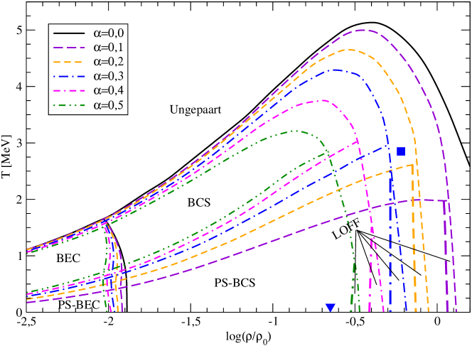
Abbildung 1: Das Phasendiagramm von Kernmaterie im Isospin-Singulett Spin-Triplett ${}^{3}S_{1}$-${}^{3}D_{1}$ Kanal in der Temperatur-Dichte Ebene für verschiedene Isospin-Asymmetrien $\alpha$ aus [18]. Wir sehen vier Phasen: die ungepaarte Phase, die BCS (BEC) Phase, die LOFF Phase und die PS (PS-BCS und PS-BEC) Phase. Für genügend kleine Asymmetrien sehen wir zwei trikritische Punkte. Für einen bestimmten Wert der Asymmetrie fallen diese beiden Werte zusammen und wir erhalten einen tetrakritischen Punkt, dargestellt durch ein blaues Quadrat. Das blaue Dreieck zeigt den Punkt der niedrigsten Dichte und gleichzeitig höchsten Asymmetrie, an dem die LOFF Phase existiert.

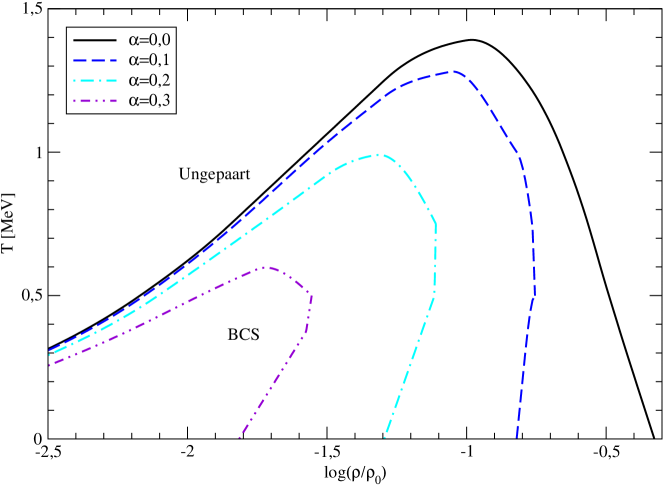
Abbildung 2: Das Phasendiagramm von Neutronenmaterie im Isospin-Triplett Spin-Singulett ${}^{1}S_{0}$ Kanal in der Temperatur-Dichte Ebene für verschiedene Spin-Asymmetrien $\alpha$. Wir sehen die ungepaarte Phase und die BCS Phase.

Crossover von BCS nach BEC

Fermionische Supraflüssigkeiten, die im Grenzfall schwacher Kopplung ein BCS aus schwach gebundenen Cooper-Paaren bilden, gehen über in ein Bose-Einstein-Kondensat (englisch: Bose-Einstein condensate) (BEC) aus stark gebundenen bosonischen Dimeren, wenn die Stärke der Paarung ausreichend groß wird [23, 24]. Für Paarung im ${}^{3}S_{1}$-${}^{3}D_{1}$ Kanal erhalten wir ein BEC aus Deuteronen im Grenzfall starker Kopplung [25, 9, 26, 27, 28, 11, 29, 30, 31, 32, 12, 33, 34, 35].

Im Grenzfall hoher Dichten erhalten wir Paarung ungebundener Teilchen im BCS. Die Paarung erfolgt hierbei an der Fermikante, die Kopplungsstärke ist schwach. Das mittlere chemische Potenzial der beiden Paarungspartner $\bar{\mu}$ ist größer als null. Wenn wir die Dichte verringern, verringert sich auch das mittlere chemische Potenzial. Bei geringen Dichten erhalten wir ein BEC aus gebundenen Teilchen mit negativem mittlerem chemischen Potenzial. Hierbei ist die Kopplungsstärke groß.

Ein weiteres Kriterium für den Crossover ist das Verhältnis des mittleren Teilchenabstandes $d$ und dem Abstand von zwei gepaarten Teilchen $\xi$. Dies ist in Abbildung 3 dargestellt. Rechts sehen wir die Situation, in der ein BCS Bereich vorkommt, hierbei gibt es Paarung an der Fermifläche von zwei Teilchen, die eine große räumliche Distanz haben; $\xi\gg d$. Links sehen wir stark gebundene Paare, die räumlich von den anderen Paaren isoliert sind; $\xi\ll d$.

Ein BEC kann nicht in jedem Paarungskanal entstehen. Im ${}^{3}S_{1}$-${}^{3}D_{1}$ Kanal können gebundene Paare entstehen; im Grenzfall verschwindender Dichte erhalten wir gebundene Deuteronen. Im ${}^{1}S_{0}$ Kanal können keine gebundenen Paare entstehen; im Grenzfall verschwindender Dichte erhalten wir freie Neutronen. Einen Übergangsbereich kann man trotzdem nachweisen [13, 14, 11].

Der Übergang von einem BCS zu einem BEC ist kein Phasenübergang, weil keine Symmetrie gebrochen wird. Es handelt sich vielmehr um Grenzfälle des gleichen Phänomens.

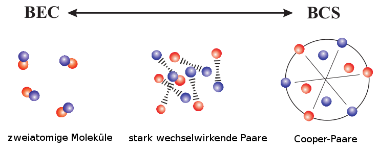
Abbildung 3: Eine Darstellung des Crossovers übernommen aus [36]. Links sehen wir gebundene Deuteronen, rechts sehen wir ungebundene Cooper-Paare.

Exotische Phasen

Neben der ungepaarten Phase und der BCS Phase haben wir exotische Phasen untersucht. Zum einen eine Phase, bei der die Cooper-Paare einen endlichen Schwerpunktsimpuls haben [37, 38, 11]. Diese Phase ist analog zur Larkin-Ovchinnikov-Fulde-Ferrell (LOFF) Phase in elektrischen Supraleitern [39, 40]. Wir hatten gesehen, dass man für eine Paarung überlappende Fermikanten benötigt. Diese Fermikanten nähern sich Stufenfunktionen für hohe Dichten und tiefe Temperaturen und werden für hohe Asymmetrien getrennt, was eine Paarung in der BCS Phase unmöglich macht.

Eine Möglichkeit trotzdem überlappende Fermikanten zu bekommen, ist, die Fermikanten gegeneinander zu verschieben. Dies ist in Abbildung 4 dargestellt. Wir erhalten einen endlichen Cooper-Paar-Impuls ${\bm{Q}}$, der in braun dargestellt ist. Die Kreise geben die Fermiflächen von Neutronen (blau) und Protonen (rot) an. Wir sehen, dass sich die Fermiflächen durch die Verschiebung um ${\bm{Q}}$ kreuzen und es einen Bereich gibt, in dem die Fermiflächen nahe beieinander sind. Außerdem sehen wir in Schwarz den Vektor ${\bm{k}}_{F}$, der mit ${\bm{Q}}$ einen Winkel von $45\degree$ einschließt und die dazugehörigen Vektoren der Neutronen (${\bm{k}}_{n}$ blau) und Protonen (${\bm{k}}_{p}$ rot). Bei diesem Winkel kompensiert der Cooper-Paar-Impuls die Verschiebung der Fermiflächen sehr gut. Durch den Cooper-Paar-Impuls erhöht sich die kinetische Energie des Systems. Andererseits wird durch die Kondensation die Energie vermindert. Die LOFF Phase bricht die Translationssymmetrie und ist somit – im Gegensatz zum Crossover von BCS nach BEC – ein Phasenübergang. Nach unseren Rechnungen tritt die LOFF Phase in Spin-asymmetrischer Neutronenmaterie nicht auf.

Eine weitere Phase, die wir im ${}^{3}S_{1}$-${}^{3}D_{1}$ Kondensat untersucht haben, ist die Phasenseparation (PS); hier trennt sich die Materie in zwei Bereiche auf: in einen Isospin-symmetrischen Teil, in dem symmetrische BCS/BEC Paarung stattfindet und in einen ungepaarten Teil, der einen starken Neutronenüberschuss besitzt. Die Phasenseparation wurde in kalten atomaren Gasen vorgeschlagen [41]. Diese Phase gibt es – im Gegensatz zum LOFF – auch bei geringen Dichten. Den Crossover von BCS zu BEC gibt es auch in der Phasenseparation. Beim Übergang zur Phasenseparation wird auch eine Symmetrie gebrochen: Das System ist anschließend nicht mehr homogen.

Sehr interessant ist auch der Verlauf der Phasenübergänge. Wir erhalten zwei trikritische Punkte, die je nach Asymmetrie an verschiedenen Phasen angrenzen. Für bestimmte Werte von Dichte, Temperatur und Asymmetrie fallen diese beiden Punkte zusammen und wir erhalten einen tetrakritischen Punkt, an dem vier Phasen koexistieren: LOFF, PS, BCS und die ungepaarte Phase. Für die Ordnung der Phasenübergänge erhalten wir Folgendes: Fast alle Phasenübergänge sind zweiter Ordnung, weil die Änderung der Parameter glatt verläuft. Die einzige Ausnahme ist der Übergang von LOFF nach PS, dort macht der Gap einen Sprung, was einem Phasenübergang erster Ordnung entspricht.

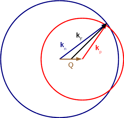
Abbildung 4: Die Fermifläche für die beiden Komponenten in der LOFF Phase. Durch die Verschiebung der Fermiflächen erhöht sich einerseits die kinetische Energie, andererseits kommt es durch den Überlapp der Fermiflächen zu einer Kondensation und somit zu einer Absenkung der Energie.

Mikroskopische Funktionen

Neben dem Verlauf des Phasendiagramms beschäftigt sich diese Arbeit auch mit mikroskopischen Funktionen. Wir haben den Gap, den Kernel der Gap-Gleichung, die Wellenfunktionen der Cooper-Paare, die Besetzungszahlen und die Einteilchenenergien berechnet. Dies haben wir sowohl für ${}^{3}S_{1}$-${}^{3}D_{1}$ Paarung als auch für ${}^{1}S_{0}$ Paarung durchgeführt. Im ${}^{3}S_{1}$-${}^{3}D_{1}$ Kanal konnten wir auch den Crossover und die LOFF Phase betrachten, im ${}^{1}S_{0}$ Kanal waren wir auf die BCS Phase beschränkt. Wir haben keine mikroskopischen Funktionen in der Phasenseparation dargestellt; da sich ein Teil der Materie in einem symmetrischen BCS/BEC befindet, kann hierbei keine neue physikalische Erkenntnis gewonnen werden.

In Abbildung 5 sehen wir den Gap als Funktion der Temperatur bei konstanter Dichte für verschiedene Asymmetrien. Oben sehen wir den ${}^{3}S_{1}$-${}^{3}D_{1}$ und unten den ${}^{1}S_{0}$ Kanal. Im ${}^{3}S_{1}$-${}^{3}D_{1}$ Kanal beziehen sich die gestrichelten Linien auf die BCS Phase und die durchgezogenen auf die resultierende Phase, BCS oder LOFF. Wir sehen, dass der Gap im ${}^{3}S_{1}$-${}^{3}D_{1}$ Kanal deutlich größer ist als im ${}^{1}S_{0}$ Kanal. Insgesamt sehen wir, dass der Gap für höhere Asymmetrien unterdrückt wird. Bei endlicher Asymmetrie und geringer Temperatur steigt der Gap für die BCS Phase mit steigender Temperatur, ansonsten fällt er. Dies liegt an dem oben beschriebenen Zusammenhang, dass die Fermikanten für hohe Asymmetrien separiert und für hohe Temperaturen aufgeweicht werden. In der LOFF Phase erhalten wir diese Anomalie nicht, weil die Fermikanten verschoben werden.

Als Nächstes wollen wir uns mit den Besetzungszahlen beschäftigen. Diese sind in Abbildung 6 für beide Paarungskanäle im BCS Limit dargestellt. Wir sehen, dass wir als grobe Struktur zwei Fermifunktionen haben, die bei $k_{F_{n/p}}/k_{F}=(1\pm\alpha)^{1/3}$ bzw. $k_{F_{\uparrow/\downarrow}}/k_{F}=(1\pm\alpha)^{1/3}$ abfallen; in der Abbildung für den ${}^{3}S_{1}$-${}^{3}D_{1}$ Kanal sind die Fermiimpulse der Neutronen und Protonen durch waagerechte schwarze Linien dargestellt. Im Fall der ${}^{3}S_{1}$-${}^{3}D_{1}$ Paarung ist das Maximum bei $2$, weil wir über den Spin summiert haben. Durch die endliche Temperatur werden die Fermifunktionen aufgeweicht. Neben der normalen Aufweichung durch die Temperatur kommt ein weiterer Effekt durch die Paarung hinzu: An der Fermikante der Minderheitskomponente fällt auch die Mehrheitskomponente ab, dann bildet sich eine Lücke aus, bis schließlich an der Fermikante der Mehrheitskomponente die Minderheitskomponente ansteigt. Wir haben sozusagen einen Abfall beider Komponenten an der Fermikante mit einer Lücke für $k_{F_{p}}\lesssim k\lesssim k_{F_{n}}$ bzw. $k_{F_{\downarrow}}\lesssim k\lesssim k_{F_{\uparrow}}$.

Diese Lücke ist auch in anderer Hinsicht von Bedeutung. Der Kernel der Gap-Gleichung liefert in diesem Bereich, in dem Paarung durch Asymmetrie unterdrückt wird, keinen Beitrag. Die Einteilchenenergien der Minderheitskomponente werden hier negativ, was zur sogenannten gapless superconductivity führt.

Beim Verringern der Dichte geht die BCS-Phase im Fall von ${}^{3}S_{1}$-${}^{3}D_{1}$ Paarung in ein BEC über. Dieser Übergang von fermionischen Eigenschaften hin zu bosonischen lässt sich bei verschiedenen untersuchten mikroskopischen Funktionen beobachten. In der LOFF Phase erhalten wir, dass der Cooper-Paar-Impuls die Aufspaltung der beiden Komponenten stark verringern kann. Insgesamt erhalten wir bei den mikroskopischen Funktionen, dass die LOFF Phase eine Annäherung an den BCS Fall mit verschwindender Asymmetrie bedeutet.

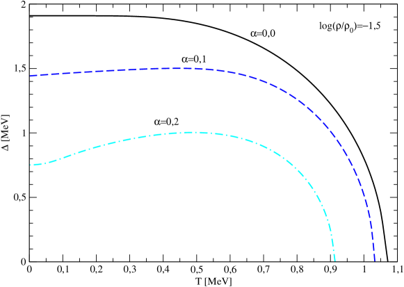
Abbildung 5: Der Gap als Funktion der Temperatur bei konstanter Dichte für verschiedene Asymmetrien. Oben für den ${}^{3}S_{1}$-${}^{3}D_{1}$ und unten für den ${}^{1}S_{0}$ Kanal. Im ${}^{3}S_{1}$-${}^{3}D_{1}$ Kanal beziehen sich die gestrichelten Linien auf die BCS Phase und die durchgezogenen Linien auf die resultierende Phase, BCS oder LOFF.

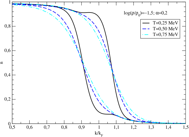
Abbildung 6: Die Besetzungszahlen der beiden Komponenten als Funktion des Impulses bei konstanter Dichte und Asymmetrie für verschiedene Temperaturen. Oben für den ${}^{3}S_{1}$-${}^{3}D_{1}$ und unten für den ${}^{1}S_{0}$ Kanal. Im ${}^{3}S_{1}$-${}^{3}D_{1}$ Kanal zeigen wir die Besetzungszahlen von Neutronen und Protonen und im ${}^{1}S_{0}$ Kanal die von Spin up und Spin down Neutronen.

Materie in starken magnetischen Feldern

Starke magnetische Felder können in kompakten Sternen auftreten [42, 43, 44, 45, 46]. Nach dem Wasserstoffbrennen entwickelt sich ein Stern, je nach Masse, zu einem Roten Riesen oder Roten Überriesen. Nach der Entwicklung über einen planetarischer Nebel bzw. eine Supernova entsteht ein kompakter Stern: ein Weißer Zwerg, ein Neutronenstern oder ein Schwarzes Loch. Das Oberflächenmagnetfeld von Weißen Zwergen beträgt $B\approx 10^{6}-10^{8}\,$G, das von Neutronensternen beträgt $B\approx 10^{12}\,$G [47]. Es wurden Neutronensterne mit Oberflächenmagnetfeldern von $B\approx 10^{14}-10^{15}\,$G entdeckt; diese Neutronensterne werden als Magnetare bezeichnet. Es wird vermutet, dass sie in ihrem Inneren Magnetfelder mit $B\approx 10^{18}\,$G haben können [42, 43, 44, 45, 47]. Aufgrund des Virialsatzes kann das Magnetfeld im Inneren eines Neutronensterns einen Wert von $B\approx 10^{18}\,$G und im Inneren von Weißen Zwergen einen Wert von $B\approx 10^{12}\,$G nicht überschreiten [47]. Starke Magnetfelder ($B\approx 10^{16}-10^{17}\,$G) werden in neugeborenen Neutronensternen in Betracht gezogen [46]. Die Zusammensetzung der Elemente in der Kruste von Neutronensternen kann durch starke Magnetfelder mit $B\gtrsim 10^{17}\,$G stark beeinflusst werden; eine aktuelle Studie über die Elementenhäufigkeit in Neutronensternen in Abhängigkeit des Magnetfeldes kann in [46] gefunden werden. Aufgrund der geringen Masse der Sterne, aus denen sich Weiße Zwerge entwickeln, bestehen Weiße Zwerge aus leichteren Elementen als die Kruste eines Neutronensterns; schwere Weiße Zwerge bestehen vermutlich zu großen Teilen aus Kohlenstoff und Wasserstoff [48]. Neon, das dritte Element, das wir in Kapitel 2 untersuchen, kommt auch in Weißen Zwergen vor. Diese relativ leichten Elemente können auch bei akkretierenden Neutronensternen vorkommen.

In Kapitel 2 und 3 untersuchen wir Materie in starken magnetischen Feldern. In Kapitel 2 untersuchen wir Kerne mit der Hartree-Fock-Theorie. Eine nähere Beschreibung findet sich z.B. in [49] und [50]; die folgende Beschreibung stützt sich auf diese Arbeiten. Der den Rechnungen aus Kapitel 2 zugrundeliegende Code ist der Sky3D Code [50]. Das ultimative Ziel bei der Beschreibung von Kernmaterie und Atomkernen ist eine Theorie, die aufgrund von grundlegenden mikroskopischen Wechselwirkungen die Eigenschaften großer Systeme voraussagen kann; die sogenannten ab inito Methoden. Für Kernmaterie und Atomkerne wären das Nukleon-Nukleon-Wechselwirkungen, bzw. die noch fundamentaleren Quantenchromodynamik (QCD) Wechselwirkungen. Derartige Modelle sind zwar für Coulomb Wechselwirkungen realisiert, aber nicht für Kernmaterie, weswegen man Näherungen machen muss. Das andere Extrem ist das Flüssigkeitstropfen-Modell (englisch: liquid-drop model) (LDM). Hierbei werden makroskopische Daten gefittet. Zwischen diesen beiden Extremen gibt es verschiedene Ansätze, z.B. Rechnungen mit einem selbstkonsistenten mittleren Feld (englisch: self-consistent mean-field) (SCMF). Diese Modelle arbeiten auf einem mikroskopischem Level, verwenden aber auch effektive Wechselwirkungen, z.B. wie in unserem Fall Skyrme-Kräfte, die eine verschwindende Reichweite haben.

In Kapitel 3 untersuchen wir suprafluide Neutronenmaterie in starken magnetischen Feldern. Vieles deckt sich mit den Untersuchungen suprafluider Kernmaterie aus Kapitel 1, diese Effekte sind weiter oben bereits erklärt. Studien zu Neutron-Neutron-Paarung finden sich z.B. in [11, 12, 13, 14, 15, 16, 17]. Neutron-Neutron-Paarung tritt auf, wenn die Isospin-Asymmetrie groß genug ist, um die dominante ${}^{3}S_{1}$-${}^{3}D_{1}$ Paarung von Neutron-Proton-Paaren zu unterdrücken. Neutron-Neutron-Paarung im ${}^{3}S_{1}$-${}^{3}D_{1}$ Kanal ist aufgrund des Pauli-Prinzips verboten. Der dominante Kanal für Neutron-Neutron-Paarung bei niedrigen Dichten ist der ${}^{1}S_{0}$ Kanal. Dieser Spin-Singulett Kanal wird durch eine Spin-Asymmetrie, die z.B. durch ein Magnetfeld verursacht wird, unterdrückt.

Kerne in starken magnetischen Feldern

Der in Sky3D gegebene Hamiltonian, der in Anhang B.4 näher beschrieben wird, hat die folgende Form:

$$\hat{h}_{q} = U_{q}(\bm{r})-\nabla\cdot\left[B_{q}(\bm{r})\nabla\right]+\mathrm{i}\bm{W}_{q}\cdot\left({\bm{\sigma}}\times\nabla\right)+{\bm{S}}_{q}\cdot{\bm{\sigma}}$$ (4)

$$-\tfrac{\mathrm{i}}{2}\left[\left(\nabla\cdot\bm{A}_{q}\right)+2\bm{A}_{q}\cdot\nabla\right]\,,$$

wobei $q$ den Isospin bezeichnet.

Um Kerne in starken magnetischen Feldern zu untersuchen, haben wir diesen Hamiltonian wie folgt modifiziert:

$$\hat{h}_{\mathrm{mod},\,q} = \hat{h}_{q}+\hat{h}_{\mathrm{mag},\,q}\,,$$ (5a)

$$\hat{h}_{\mathrm{mag},\,q} = -\left({\bm{l}}\cdot\delta_{q,p}+g_{q}\frac{{\bm{\sigma}}}{2}\right)\cdot\tilde{\bm{B}}_{q}\,,$$ (5b)

hierbei bezeichnet $g_{q}$ den Landé $g$-Faktor und $\tilde{\bm{B}}_{q}=e\hbar/(2m_{q}c){\bm{B}}$. Der erste Term berücksichtigt die Kopplung des Bahndrehimpulses an das Magnetfeld und der zweite die des Spins. Eine nähere Erklärung von Gleichung (5b) befindet sich in Unterabschnitt 2.3.1.

In Abbildung 7 sind verschiedene Quantenzahlen für Spin und Bahndrehimpuls dargestellt. Hierbei haben wir $s$- und $p$-Zustände berücksichtigt. Da wir Spin-$1/2$-Teilchen haben, ist der Spin $s$ immer $1/2$ und somit gilt für die $z$-Komponente $m_{s}=\uparrow,\,\downarrow$, mit $\uparrow=+1/2$ und $\downarrow=-1/2$. Bei $s$-Zuständen erhalten wir für den Bahndrehimpuls $l=0$, somit gilt für die $z$-Komponente $m_{l}=0$. Folglich haben wir zwei Zustände, nämlich die in Abbildung 7 rot bzw. braun dargestellten Pfeile. Bei $p$-Zuständen haben wir $l=1$ und somit drei Möglichkeiten für $m_{l}$: $m_{l}=-1,\,0,\,1$. Für Zustände mit $M=\pm 3/2$ haben wir je eine Möglichkeit, für Zustände mit $M=\pm 1/2$ haben wir je zwei Möglichkeiten; die entsprechenden Einteilchenzustände berechnen sich aus Superpositionen dieser Zustände.

Im Folgenden wollen wir unsere Resultate kurz zusammenfassen; eine ausführliche Darstellung findet sich in Unterabschnitt 2.3.3.

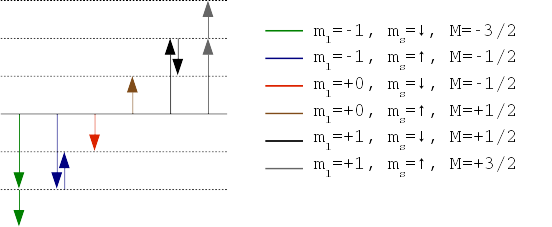
Abbildung 7: Die Quantenzahlen für verschiedene Zustände. $m_{l}$ bezeichnet die $z$-Komponente des Bahndrehimpulses, $m_{s}$ die des Spins und $M$ ist deren Summe.

Energieniveaus, Bahndrehimpuls und Spin

In den Abbildungen 8 und 9 sind verschiedene Größen für Protonen und Neutronen in [16]O dargestellt. Links unten sehen wir jeweils die Energieniveaus der einzelnen Einteilchenzustände. Die $s_{1/2}$, $p_{3/2}$ und $p_{1/2}$ Zustände sind bei verschwindendem Magnetfeld jeweils entartet und spalten sich bei nicht verschwindendem Magnetfeld auf. Bei $B=4.0\cdot 10^{17}\,$G erhalten wir eine Umbesetzung der Energieniveaus. Für $\left<L_{z}\right>$ und $\left<S_{z}\right>$ erhalten wir halb- bzw. ganzzahlige Werte für alle $s$-Zustände und $p$-Zustände mit $M=\pm 3/2$; für $p$-Zustände mit $M=\pm 1/2$ erhalten wir Superpositionen, wie oben erklärt. Bei Letzteren haben wir zwei Effekte: die Spin-Bahn-Kopplung und die Kopplung des Bahndrehimpulses und des Spins einzeln an das Magnetfeld. Ersteres dominiert bei schwachen, Letzteres bei starken Magnetfeldern. Deswegen erhalten wir halb- bzw. ganzzahlige Werte nur im Grenzfall starker Magnetfelder. Der Grenzfall schwacher Magnetfelder wird durch den Zeeman-Effekt und der Grenzfall starker Magnetfelder durch den Paschen-Back-Effekt beschrieben.

Abbildung 8: Die Energieniveaus (gestrichelte Linie: analytisch, durchgezogene Linie: numerisch), $\left<L_{z}\right>$ und $\left<S_{z}\right>$ als Funktionen des Magnetfeldes für Protonen in [16]O.

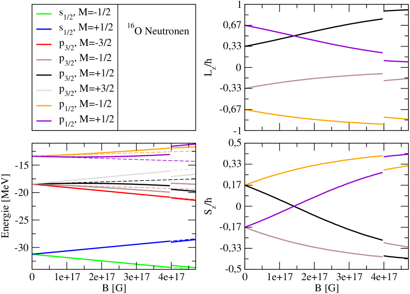
Abbildung 9: Die Energieniveaus (gestrichelte Linie: analytisch, durchgezogene Linie: numerisch), $\left<L_{z}\right>$ und $\left<S_{z}\right>$ als Funktionen des Magnetfeldes für Neutronen in [16]O.

Spin- und Stromdichte

Als Nächstes wollen wir auf die Spin- und die Stromdichte anhand von [12]C eingehen. In Abbildung 10 ist die normierte Stromdichte (kollektive Fließgeschwindigkeit) dargestellt. Das Magnetfeld ist in beiden Fällen $B=4{,}1\cdot 10^{17}\,$G, die linke Abbildung stellt Neutronen und die rechte Protonen dar. Wir sehen, dass die kollektive Fließgeschwindigkeit senkrecht zum Magnetfeld verläuft. Außerdem sehen wir, dass die kollektive Fließgeschwindigkeit der Protonen und Neutronen in verschiedene Richtungen verläuft. Dies liegt an den unterschiedlichen Vorzeichen von $g_{n}$ und $g_{p}$.

In Abbildung 11 sehen wir die normierte Spindichte für Protonen bei zwei verschiedenen Magnetfeldern: Links ist das Magnetfeld verhältnismäßig sehr klein ($B=4{,}0\cdot 10^{13}\,$G) und rechts groß ($B=4{,}1\cdot 10^{17}\,$G). Hier sehen wir die Ausrichtung des Spins bei zunehmendem Magnetfeld; bei kleinem Magnetfeld ist der Spin aufgrund der dominanten Spin-Bahn-Kopplung wenig ausgerichtet, wohingegen die Ausrichtung bei starkem Magnetfeld deutlich zu sehen ist.

Abbildung 10: Die Stromdichte dividiert durch die Teilchendichte (kollektive Fließgeschwindigkeit) für [12]C für $B=4{,}1\cdot 10^{17}\,$G mit der Teilchendichte im Hintergrund für Neutronen (links) und Protonen (rechts). Diese Abbildung wurde mit VisIt [51] erstellt.

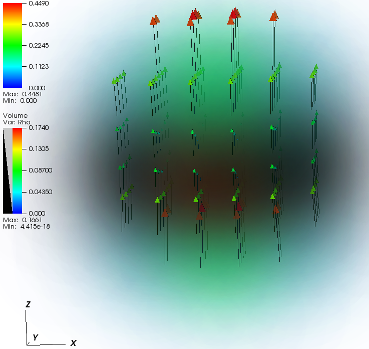
Abbildung 11: Die Spindichte dividiert durch die Teilchendichte für [12]C mit der Teilchendichte im Hintergrund für Protonen für verschiedene Magnetfelder: $B=4{,}0\cdot 10^{13}\,$G (links) und $B=4{,}1\cdot 10^{17}\,$G (rechts). Diese Abbildung wurde mit VisIt [51] erstellt.

Verformung

In Abbildung 12 sehen wir die Verformung von [20]Ne, das Magnetfeld nimmt von links nach rechts zu. Bei $B=0$ ist der Atomkern stark verformt, mit zunehmendem Magnetfeld nimmt die Verformung ab.

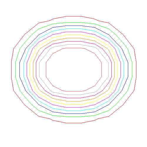
Abbildung 12: Der verformte Atomkerne [20]Ne für $B=0$, $B=2{,}4\cdot 10^{17}\,$G und $B=4{,}9\cdot 10^{17}\,$G. Diese Abbildung wurde mit VisIt [51] erstellt.

Neutronenmaterie in starken magnetischen Feldern

Neutronensternmaterie kann in erster Näherung als reine Neutronenmaterie behandelt werden [16], weil der Anteil von Protonen und Elektronen und schweren Barionen nicht mehr als $5\%$-$10\%$ der Gesamtdichte des Systems ausmacht. Daher spielt Neutron-Neutron-Paarung eine wichtige Rolle in der Physik der inneren Kruste eines Neutronensterns. Außerdem spielt sie eine wichtige Rolle für Neutronen-reiche Atomkerne in der Nähe der Drip Line (Kerne, die keine Neutronen mehr binden können.) [13]. Es gibt ein paar phänomenologische Hinweise auf Neutronen-Suprafluidität in Neutronensternen. Bekannte Beispiele sind Periodensprünge (englisch: glitches) in dem Rotationsverhalten einiger Pulsare und das Kühlungsverhalten des jüngsten bekannten Neutronensterns in Kassiopeia A [17].

Neben dem oben erwähnten Phasendiagramm und den mikroskopischen Funktionen haben wir den Einfluss des Magnetfeldes auf die Spin-Asymmetrie (Polarisation) untersucht. Außerdem haben wir die magnetische Energie mit der Temperatur verglichen. In Abbildung 13 ist das Magnetfeld, das für eine bestimmte Polarisation benötigt wird, als Funktion der Dichte dargestellt. Verschiedene Felder zeigen verschiedene Werte der Polarisation, verschiedene Farben stehen für verschiedene Temperaturen. Wir sehen, dass das benötigte Magnetfeld in der Regel für steigende Polarisation, steigende Dichte oder fallende Temperatur steigt.

In Abbildung 14 sehen wir die magnetische Energie $\varepsilon_{B}$ mit

$$\varepsilon_{B} = |\tilde{\mu}_{n}B|$$ (6)

dividiert durch die Temperatur $T$. Wir sehen, dass $\varepsilon_{B}$ in der Regel größer ist als $T$. Formel 6 wird in Abschnitt 3.2 näher erklärt.

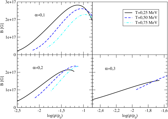
Abbildung 13: Das Magnetfeld, das benötigt wird, um eine bestimmte Spin-Asymmetrie (Polarisation) zu erzeugen, als Funktion der Dichte. In jedem Feld ist eine bestimmte Polarisation fixiert. Verschiedene Temperaturen sind mit verschiedenen Farben dargestellt.

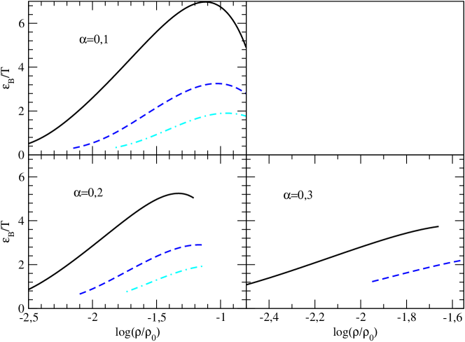
Abbildung 14: Die magnetische Energie dividiert durch die Temperatur als Funktion der Dichte für verschiedene Temperaturen und Polarisationen. Der Farbcode ist der gleiche wie in Abbildung 13.

Schlußfolgerungen

In Kapitel 1 untersuchen wir Kernmaterie bei niedrigen Dichten, tiefen Temperaturen und nicht verschwindender Isospin-Asymmetrie. Hierbei erhalten wir ein reichhaltiges Phasendiagramm bestehend aus der translations- und rotationssymmetrischen BCS Phase, einem BEC bestehend aus Neutron-Proton-Dimeren und den exotischen Phasen LOFF und PS. Wir erhalten zwei trikritische Punkte, die für einen bestimmten Wert von Dichte, Temperatur und Asymmetrie in einem tetrakritischen Punkt zusammenfallen können. Außerdem existieren zwei Crossovers: bei hohen Temperaturen von einer asymmetrischen BCS Phase zu einem von BEC, das von einem Neutronengas umgeben ist. Bei tiefen Temperaturen erhalten wir einen Crossover in der Phasenseparation. Wir haben verschiedene mikroskopische Funktionen untersucht – den Gap, den Kernel der Gap-Gleichung, die Wellenfunktionen der Cooper-Paare, die Besetzungszahlen und die Einteilchenenergien. Hierbei konnten wir den Übergang von einer schwach gebundenen BCS-Phase bei hohen Dichten zu einem stark gebundenen BEC bei niedrigen Dichten beobachten. Wir konnten auch sehen, dass sich die mikroskopischen Funktionen der LOFF Phase denen der BCS-Phase bei verschwindender Asymmetrie annähern. Außerdem konnten wir eine Lücke um die Fermikante herum feststellen, die sich auf die mikroskopischen Funktionen auswirkt.

In Kapitel 2 untersuchen wir den Einfluss von starken Magnetfeldern auf verschiedene Atomkerne mit einem Skyrme-Hartree-Fock (SHF) Ansatz unter Benutzung des Codes Sky3D. Starke Magnetfelder können z.B. in Neutronensternen realisiert werden. Die Elemente, die wir untersuchen, kommen in Weißen Zwergen vor, die auch starke Magnetfelder haben können. Wir haben drei verschiedene Atomkerne betrachtet: [16]O, [12]C und [20]Ne. Wir haben den Spin und den Bahndrehimpuls als Funktion des Magnetfeldes untersucht; bei schwachen Magnetfeldern ist deren Ausrichtung aufgrund der dominierenden Spin-Bahn-Wechselwirkung gering, bei starken Magnetfeldern dominiert die Kopplung von Spin- und Bahndrehimpuls an das Magnetfeld. Bei [16]O haben wir eine Umbesetzung der Energieniveaus bei starken Magnetfeldern sehen können. Bei [20]Ne konnten wir erkennen, dass die Verformung mit zunehmendem Magnetfeld abnimmt.

In Kapitel 3 untersuchen wir Neutronenmaterie und erhalten ein Phasendiagramm für Spin-asymmetrische (polarisierte) Materie, das dem aus Kapitel 1 zwar sehr ähnelt, aber einige Unterschiede aufweist. Dadurch, dass der Paarungskanal schwächer ist, erhalten wir geringere kritische Temperaturen. Außerdem erhalten wir kein BEC und keine LOFF Phase. Die Berechnungen der mikroskopischen Funktionen in der BCS-Phase sind mit denen aus Kapitel 1 vergleichbar. Durch das Ausbleiben der LOFF Phase erhalten wir eine untere kritische Temperatur. Wir haben auch untersucht, welche Magnetfeldstärken welche Polarisation verursachen. Außerdem haben wir die magnetische Energie mit der Temperatur verglichen; hierbei war die magnetische Energie in der Regel größer als die der Temperatur.

Perspektiven

Die Rechnungen in Kapitel 1 gehen von Neutron-Proton-Paarung und zusätzlichen Neutronen aus. Die Rechnungen könnten durch Einbeziehen von Clustern verbessert werden. Des Weiteren könnte man die Rechnungen aus den Kapiteln 1 und 3 kombinieren, indem sowohl Isospin-Singulett Spin-Triplett Paarung als auch Isospin-Triplett Spin-Singulett Paarung in die Rechnungen eingebaut werden. Hierbei ist zu erwarten, dass bei einer bestimmten Isospin-Asymmetrie ein Phasenübergang von Isospin-Singulett Spin-Triplett Paarung zu Isospin-Triplett Spin-Singulett Paarung erfolgt.

Die Ergebnisse, die in Kapitel 2 gezeigt werden, können in Zukunft auf verschiedene Weisen verbessert werden. Ein verbesserter Hamiltonian könnte verwendet werden; insbesondere könnten Spin-Spin-Wechselwirkungen in Hinblick auf starke magnetische Felder interessant sein. Außerdem könnten Methoden entwickelt werden, die die aktuellen Studien in den Bereich stärkerer Magnetfelder oder schwererer Atomkerne ausdehnen.

Abstract

This PhD thesis deals with nuclear matter and nuclei under extreme conditions. These can occur e.g. in compact stars. Chapter 1 studies superfluid neutron-proton pairing in isospin-asymmetric nuclear matter in the ${}^{3}S_{1}$-${}^{3}D_{1}$ channel. In chapter 2 we study the influence of strong magnetic fields on [12]C, [16]O and [20]Ne. Finally, we study in chapter 3 superfluid neutron-neutron pairing in spin-asymmetric (polarized) neutron matter in the ${}^{1}S_{0}$ channel; a polarization can be induced e.g. by a magnetic field.

In chapter 1 we obtain a rich phase diagram for isospin-asymmetric nuclear matter. A better understanding of this matter can be important e.g. for low energy heavy ion collisions, supernovae explosions or nuclei. In the outer area of nuclei the density is low, thus an isospin-asymmetry hardly suppresses neutron-proton pairing. We study the unpaired phase and several superfluid phases. We study the crossover from the weakly coupled Bardeen Cooper Schrieffer (BCS) phase at high densities to the Bose-Einstein condensate (BEC) in the limit of strong coupling at low densities. Moreover, we study two exotic phases: the Larkin-Ovchinnikov-Fulde-Ferrell (LOFF) phase, at which Cooper-pairs get a nonvanishing center-of-mass momentum. This phase exists only at high densities. Moreover, we study a phase separation (PS) consisting of an isospin symmetric BCS or BEC part and an isospin asymmetric unpaired part with neutron excess. The phase separation can exist both at high and low densities, thus we obtain a crossover in the phase separation. The phase transition between LOFF and PS is of first order, all other phase transitions are of second order. Furthermore, we study the gap, the kernel of the gap equation, the Cooper-pair wave functions, the occupation numbers and the quasiparticle dispersion relations. In the BCS limit, we obtain a fermionic and in the BEC limit a bosonic nature. For the LOFF phase the intrinsic features approach those of the BCS phase at vanishing isospin asymmetry.

In chapter 2 we study the effect of a strong magnetic field on the elements [16]O, [12]C and [20]Ne. These elements can occur e.g. in white dwarfs, which can have strong magnetic fields. Furthermore, these elements can play an important role for accreting neutron stars. For [16]O and [12]C the single particle energies are splitted with increasing magnetic field. Moreover, the $z$-component of the angular momentum and the spin are aligned with the magnetic field at strong magnetic fields, this alignment is suppressed by the spin-orbit coupling for weak magnetic fields. In [16]O the energy states are rearranged at strong magnetic fields. For the collective flow velocity in the nuclei we obtain circular or almost circular orbits around the axis of the magnetic field. The spin density aligns with the magnetic field for strong mangetic fields. [20]Ne is strongly deformed at vanishing magnetic fields, this deformation decreases with increasing magnetic field.

The phase diagram for polarized neutron matter studied in chapter 3 can be of great importance for studies of neutron matter; in particular for the inner crust of neutron stars. It can also be important for studies on nuclei. There are some phenomenological indications of neutron superfluidity in neutron stars. The obtained phase diagram consists only of the unpaired phase and the BCS phase. Since there exists no bound neutron-neutron pairs, BEC cannot form. Since the coupling strength of the ${}^{1}S_{0}$ channel is weaker than the one of the ${}^{3}S_{1}$-${}^{3}D_{1}$ channel, the critical temperature is lower than in the phase diagram analyzed in chapter 1. For the intrinsic features we obtain similar results as for the BCS phase in chapter 1. Moreover, we have studied the magnetic field needed for a certain magnetization and compared its energy with the temperature of the system. In the sector we studied, the magnetic energy is normally greater than the temperature.

Table of Contents

1. 1 BCS-BEC crossovers and unconventional phases in dilute nuclear matter
   1. 1.1 Introduction
   2. 1.2 Theory
   3. 1.3 BCS-phase, LOFF phase and crossover to BEC
      1. 1.3.1 Phase diagram
      2. 1.3.2 Temperature and asymmetry dependence of the gap: contrasting the BCS and LOFF phases
      3. 1.3.3 Occupation numbers and chemical potentials
      4. 1.3.4 Effects of finite momentum in the LOFF phase
      5. 1.3.5 The kernel of the gap equation
      6. 1.3.6 The Cooper-pair wave function across the BCS-BEC crossover
      7. 1.3.7 Occupation numbers across the BCS-BEC crossover
      8. 1.3.8 Quasiparticle spectra
   4. 1.4 Conclusion
2. 2 Hartree-Fock
   1. 2.1 Introduction
   2. 2.2 Overview of the TDHF Code
      1. 2.2.1 Introduction
      2. 2.2.2 Physics implemented in the code
   3. 2.3 Hartree-Fock with magnetic field
      1. 2.3.1 Introduction
      2. 2.3.2 Clebsch-Gordan coefficients
      3. 2.3.3 Results
      4. 2.3.4 Outlook
   4. 2.4 Conclusion
3. 3 BCS pairing in neutron matter
   1. 3.1 Introduction
   2. 3.2 Theory
   3. 3.3 Results
      1. 3.3.1 Phase diagram
      2. 3.3.2 Intrinsic features
      3. 3.3.3 Magnetic field strength
   4. 3.4 Conclusion
4. A Matsubara summations
5. B Description of the TDHF Code
   1. B.1 Local densities and currents
   2. B.2 The energy-density functional
   3. B.3 Force coefficients
   4. B.4 The single-particle Hamiltonian
   5. B.5 Static Hartree-Fock
   6. B.6 Observables

List of Figures

1. 1 Das Phasendiagramm von Kernmaterie im Isospin-Singulett Spin-Triplett ${}^{3}S_{1}$-${}^{3}D_{1}$ Kanal in der Temperatur-Dichte Ebene für verschiedene Isospin-Asymmetrien $\alpha$ aus [18]. Wir sehen vier Phasen: die ungepaarte Phase, die BCS (BEC) Phase, die LOFF Phase und die PS (PS-BCS und PS-BEC) Phase. Für genügend kleine Asymmetrien sehen wir zwei trikritische Punkte. Für einen bestimmten Wert der Asymmetrie fallen diese beiden Werte zusammen und wir erhalten einen tetrakritischen Punkt, dargestellt durch ein blaues Quadrat. Das blaue Dreieck zeigt den Punkt der niedrigsten Dichte und gleichzeitig höchsten Asymmetrie, an dem die LOFF Phase existiert.
2. 2 Das Phasendiagramm von Neutronenmaterie im Isospin-Triplett Spin-Singulett ${}^{1}S_{0}$ Kanal in der Temperatur-Dichte Ebene für verschiedene Spin-Asymmetrien $\alpha$. Wir sehen die ungepaarte Phase und die BCS Phase.
3. 3 Eine Darstellung des Crossovers übernommen aus [36]. Links sehen wir gebundene Deuteronen, rechts sehen wir ungebundene Cooper-Paare.
4. 4 Die Fermifläche für die beiden Komponenten in der LOFF Phase. Durch die Verschiebung der Fermiflächen erhöht sich einerseits die kinetische Energie, andererseits kommt es durch den Überlapp der Fermiflächen zu einer Kondensation und somit zu einer Absenkung der Energie.
5. 5 Der Gap als Funktion der Temperatur bei konstanter Dichte für verschiedene Asymmetrien. Oben für den ${}^{3}S_{1}$-${}^{3}D_{1}$ und unten für den ${}^{1}S_{0}$ Kanal. Im ${}^{3}S_{1}$-${}^{3}D_{1}$ Kanal beziehen sich die gestrichelten Linien auf die BCS Phase und die durchgezogenen Linien auf die resultierende Phase, BCS oder LOFF.
6. 6 Die Besetzungszahlen der beiden Komponenten als Funktion des Impulses bei konstanter Dichte und Asymmetrie für verschiedene Temperaturen. Oben für den ${}^{3}S_{1}$-${}^{3}D_{1}$ und unten für den ${}^{1}S_{0}$ Kanal. Im ${}^{3}S_{1}$-${}^{3}D_{1}$ Kanal zeigen wir die Besetzungszahlen von Neutronen und Protonen und im ${}^{1}S_{0}$ Kanal die von Spin up und Spin down Neutronen.
7. 7 Die Quantenzahlen für verschiedene Zustände. $m_{l}$ bezeichnet die $z$-Komponente des Bahndrehimpulses, $m_{s}$ die des Spins und $M$ ist deren Summe.
8. 8 Die Energieniveaus (gestrichelte Linie: analytisch, durchgezogene Linie: numerisch), $\left<L_{z}\right>$ und $\left<S_{z}\right>$ als Funktionen des Magnetfeldes für Protonen in [16]O.
9. 9 Die Energieniveaus (gestrichelte Linie: analytisch, durchgezogene Linie: numerisch), $\left<L_{z}\right>$ und $\left<S_{z}\right>$ als Funktionen des Magnetfeldes für Neutronen in [16]O.
10. 10 Die Stromdichte dividiert durch die Teilchendichte (kollektive Fließgeschwindigkeit) für [12]C für $B=4{,}1\cdot 10^{17}\,$G mit der Teilchendichte im Hintergrund für Neutronen (links) und Protonen (rechts). Diese Abbildung wurde mit VisIt [51] erstellt.
11. 11 Die Spindichte dividiert durch die Teilchendichte für [12]C mit der Teilchendichte im Hintergrund für Protonen für verschiedene Magnetfelder: $B=4{,}0\cdot 10^{13}\,$G (links) und $B=4{,}1\cdot 10^{17}\,$G (rechts). Diese Abbildung wurde mit VisIt [51] erstellt.
12. 12 Der verformte Atomkerne [20]Ne für $B=0$, $B=2{,}4\cdot 10^{17}\,$G und $B=4{,}9\cdot 10^{17}\,$G. Diese Abbildung wurde mit VisIt [51] erstellt.
13. 13 Das Magnetfeld, das benötigt wird, um eine bestimmte Spin-Asymmetrie (Polarisation) zu erzeugen, als Funktion der Dichte. In jedem Feld ist eine bestimmte Polarisation fixiert. Verschiedene Temperaturen sind mit verschiedenen Farben dargestellt.
14. 14 Die magnetische Energie dividiert durch die Temperatur als Funktion der Dichte für verschiedene Temperaturen und Polarisationen. Der Farbcode ist der gleiche wie in Abbildung 13.
15. 1.1 The elastic scattering phase shifts and the critical temperatures of pairing in the attractive interaction channels.
16. 1.2 Phase diagram of isospin asymmetric nuclear matter.
17. 1.3 The gap of various phases, the LOFF momentum and the PS filling fraction
18. 1.4 Illustration of the crossover.
19. 1.5 The zoomed crossover region of the phase diagram.
20. 1.6 Illustration of temperature induced smearing of the Fermi surfaces.
21. 1.7 The gap as a function of the temperature.
22. 1.8 The gap as a function of the asymmetry.
23. 1.9 The neutron and proton occupation numbers for several temperatures in the BCS phase.
24. 1.10 Chemical potentials of neutrons and protons for several temperatures in the BCS/BEC phase.
25. 1.11 Illustration of the mechanism of phase-space restoration by the LOFF phase.
26. 1.12 Properties of the nuclear LOFF phase. Pairing gaps and the corresponding free energies are shown as functions of the total momentum of a Cooper-pair.
27. 1.13 Dependence of the kernel on momentum for various densities.
28. 1.14 Dependence of the kernel on momentum for various temperatures.
29. 1.15 Dependence of the kernel on momentum for various asymmetries.
30. 1.16 Dependence of the kernel on momentum in the BCS and the LOFF phase.
31. 1.17 Dependence of the kernel on momentum in the LOFF phase for different angles.
32. 1.18 Dependence of $\Psi(r)$ on $r$ for the three coupling regimes.
33. 1.19 Dependence of $r^{2}|\Psi(r)|^{2}$ on $r$ for the three coupling regimes.
34. 1.20 Dependence of $\Psi(r)$ and $r^{2}|\Psi(r)|^{2}$ on $r$ in the LOFF phase in the WCR for three different angles and two different asymmetries.
35. 1.21 Dependence of $\Psi(r)$ on $r$ in the LOFF phase in the WCR for two different angles and one asymmetry.
36. 1.22 Dependence $r^{2}|\Psi(r)|^{2}$ on $r$ in the LOFF phase in the WCR for two different angles and one asymmetry.
37. 1.23 Dependence of $\Psi(r)$ and $r^{2}|\Psi(r)|^{2}$ on $r$ in the LOFF phase in the WCR integrated over the angle for two asymmetries.
38. 1.24 Dependence of the neutron and proton occupation numbers on momentum for the three coupling regimes.
39. 1.25 Dependence of the neutron and proton occupation numbers on momentum in the LOFF phase in the WCR for two asymmetries and three angles.
40. 1.26 Dispersion relations for quasiparticle spectra in the case of the BCS condensate, as functions of momentum.
41. 1.27 Dispersion relations for quasiparticle spectra in the LOFF phase in the WCR, as functions of momentum for three angles.
42. 1.28 Illustration of Fermi surfaces in the LOFF phase.
43. 2.1 Spin and orbit angular momentum quantum numbers of $s$- and $p$-states.
44. 2.2 The energy levels, $\left<L_{z}\right>$ and $\left<S_{z}\right>$ as functions of the magnetic field for protons in ¹⁶O.
45. 2.3 The energy levels, $\left<L_{z}\right>$ and $\left<S_{z}\right>$ as functions of the magnetic field for neutrons in ¹⁶O.
46. 2.4 The energy levels as functions of the magnetic field for neutrons and protons in ¹²C.
47. 2.5 The angular momentum and the spin as functions of the magnetic field for neutrons and protons in ¹²C.
48. 2.6 The $r_{\mathrm{rms}}$, $\beta$ and $\gamma$ as functions of the magnetic field for [20]Ne.
49. 2.7 Illustration of the deformed ²⁰Ne nucleus for different values of the magnetic field.
50. 2.8 The collective flow velocity for neutrons and protons for ¹⁶O for different values of the magnetic field.
51. 2.9 The spin density divided by the particle density for neutrons and protons for ¹⁶O for different values of the magnetic field.
52. 2.10 The collective flow velocity for neutrons and protons for ¹²C for different values of the magnetic field.
53. 2.11 The spin density divided by the particle density for neutrons and protons for ¹²C for different values of the magnetic field.
54. 2.12 The collective flow velocity for neutrons and protons for ²⁰Ne for different values of the magnetic field.
55. 2.13 The spin density divided by the particle density for neutrons and protons for ²⁰Ne for different values of the magnetic field.
56. 3.1 Phase diagram of spin polarized neutron matter.
57. 3.2 The gap as a function of the temperature.
58. 3.3 The gap as a function of the polarization.
59. 3.4 Dependence of the kernel on momentum for various polarizations at high density.
60. 3.5 Dependence of the kernel on momentum for various polarizations at intermediate density.
61. 3.6 Dependence of the kernel on momentum for various polarizations at low density.
62. 3.7 Dependence of the kernel on momentum for various temperatures.
63. 3.8 Dependence of $\Psi(r)$ on $r$ for three densities and four polarizations.
64. 3.9 Dependence of $r^{2}|\Psi(r)|^{2}$ on $r$ for three densities and four polarizations.
65. 3.10 Dependence of the spin-up and spin-down neutron occupation numbers on momentum for various polarizations at high density.
66. 3.11 Dependence of the spin-up and spin-down neutron occupation numbers on momentum for various polarizations at intermediate density.
67. 3.12 Dependence of the spin-up and spin-down neutron occupation numbers on momentum for various polarizations at low density.
68. 3.13 Dependence of the spin-up and spin-down neutron occupation numbers on momentum for various temperatures.
69. 3.14 Dispersion relations for quasiparticle spectra in the case of the BCS condensate, as functions of momentum.
70. 3.15 The needed magnetic field to create a certain spin-polarization as a function of the density with fixed polarisation.
71. 3.16 The needed magnetic field to create a certain spin-polarization as a function of the density with fixed temperature.
72. 3.17 The magnetic energy divided by the temperature as a function of the density with fixed polarisation.
73. 3.18 The magnetic energy divided by the temperature as a function of the density with fixed temperature.

Chapter 1 BCS-BEC crossovers and unconventional phases in dilute nuclear matter

1.1 Introduction

The vacuum two-nucleon interaction at low energies is experimentally constrained by the phase-shift data obtained from the analysis of elastic nucleon-nucleon collisions. The attractive part of the nuclear interaction which is dominant at low energies leads to a formation of nuclear clusters and the appearance of nucleonic pair condensates of the Bardeen-Cooper-Schrieffer (BCS) type at sufficiently low temperatures. Fig. 1.1 shows the scattering phase shifts as a function of laboratory energy for attractive channels (left panel) and the corresponding critical temperatures for transition to superconducting/superfluid state (right panel). The overall behavior of nuclear matter at low density is rather complex because of the possibility of the formation of clusters and condensates. The physics of low density nuclear matter is relevant for astrophysics of supernova matter and neutron stars. These settings differ in the values of additional parameters (apart from the matter density) such as temperature ($T$) and isospin asymmetry ($\alpha$). In supernovae $\alpha$ is non-zero but small compared to that of cold $\beta$-catalyzed matter in neutron stars. Under large isospin asymmetry the neutron-proton pairing is disrupted and ${}^{1}S_{0}$ pairing in the isospin-triplet, spin-singlet state of neutrons is favored. This is the case in neutron stars. In supernova matter nearly isospin-symmetrical matter supports ${}^{3}S_{1}$-${}^{3}D_{1}$ pairing in the spin-triplet, isospin-singlet state, because the isospin asymmetry is not large enough to suppress the ${}^{3}S_{1}$-${}^{3}D_{1}$ pairing.

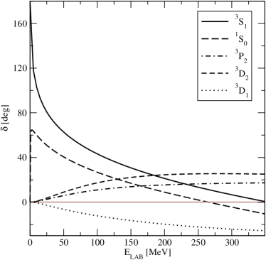
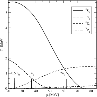
Figure 1.1: a) The elastic scattering phase shifts as a function of the laboratory energy (left panel). The critical temperatures of pairing in the attractive interaction channels (right panel). Taken from Ref. [52] (The variable $n_{0}$ of the right figure is the nuclear saturation density which is called $\rho_{0}$ in this thesis.)

Fermionic BCS superfluids, which form loosely bound Cooper-pairs in the weak-coupling limit undergo a transition to the Bose-Einstein condensate (BEC) of tightly bound bosonic dimers, when the pairing strength increases sufficiently [23, 24]. In experiments on cold atomic gases, the pairing strength can be manipulated via the Feshbach mechanism. The transition from BCS to BEC regime of pairing was confirmed experimentally in these systems. In isospin-symmetric nuclear matter, this transition may occur upon dilution of the system. If the pairing is in the ${}^{3}S_{1}$-${}^{3}D_{1}$ channel the asymptotic state of the strong-coupling limit is a BEC of deuterons [25, 9, 26, 27, 28, 11, 29, 30, 31, 32, 12, 33, 34, 35]. The isoscalar neutron-proton ($np$) pairing is disrupted by isospin asymmetry, which is induced by weak interactions in stellar environments and is expected in exotic nuclei. This disruption occurs because the mismatch in the Fermi surfaces of protons and neutrons suppresses the pairing correlations [22]. Moreover the standard Nozières-Schmitt-Rink theory [23] of the BCS-BEC crossover must also be modified in a way that the low-density asymptotic state becomes a gaseous mixture of neutrons and deuterons [53]. The ${}^{3}S_{1}$-${}^{3}D_{1}$ condensates can be important in several physical backgrounds. (i) Low-energy heavy-ion collisions produce large amounts of deuterons in final states as putative fingerprints of ${}^{3}S_{1}$-${}^{3}D_{1}$ condensation [9]. (ii) Large nuclei may feature spin-aligned $np$ pairs, as evidenced by recent experimental findings [10] on excited states in ⁹²Pd; moreover, exotic nuclei with extended halos provide a locus for $n$-$p$ Cooper pairing. (iii) Directly relevant to the parameter ranges covered in this chapter are the observations that supernova and hot proto-neutron-star matter at sub-saturation densities have low temperature and low isospin asymmetry, and that the deuteron fluid is a substantial constituent [54, 55].

Two relevant energy scales which are important for this chapter are the magnitude of the shift $\delta\mu=(\mu_{n}-\mu_{p})/2$ of the chemical potentials of neutrons $\mu_{n}$ and protons $\mu_{p}$ from their common value $\mu_{0}$ at isospin symmetry and the pairing gap $\Delta_{0}$ in the ${}^{3}S_{1}$-${}^{3}D_{1}$ channel at $\delta\mu=0$. With increasing isospin asymmetry, i.e., with $\delta\mu$ increasing from zero to values of the order for $\Delta_{0}$, several unconventional phases may emerge. One of these is a neutron-proton condensate with Cooper-pairs which have a nonzero center-of-mass (CM) momentum [37, 38, 11]. This phase is the analogue of the Larkin-Ovchinnikov-Fulde-Ferrell (LOFF) phase in electric superconductors [39, 40]. Another possible phase is the phase-separation (PS) consisting of an isospin symmetric BCS part and an isospin asymmetric unpaired part. This phase was first proposed in cold atomic gases [41]. As an alternative to the LOFF phase we could include üthe deformed Fermi surface (DFS) phase. In contrast to the LOFF phase it is translationally invariant but it breaks the rotational symmetry [56, 38]. However, these two phases have many properties in common and we concentrate only on the LOFF phase. At large isospin asymmetry, where ${}^{3}S_{1}$-${}^{3}D_{1}$ pairing is strongly suppressed, a BCS-BEC crossover may also occur in the isotriplet ${}^{1}S_{0}$ pairing channel, notably in neutron-rich systems and halo nuclei [13, 14, 15, 57, 58, 59, 60, 61]. From the experimental phase shifts we can conclude that the pairing force in the ${}^{3}S_{1}$-${}^{3}D_{1}$ channel is stronger than in the ${}^{1}S_{0}$ channel. Isotriplet, spin-triplet pairing is prohibited by the Pauli principle; accordingly, isotriplet pairing occurs only in the spin-singlet channel. Since isosinglet, spin-triplet pairing is favored over isotriplet spin-singlet pairing for not very high asymmetries, we neglect isotriplet pairing. For large asymmetries, isosinglet pairing is strongly suppressed and therefore pairing takes place mostly in the isotriplet spin-singlet channel. Thus, to conclude, for large asymmetries we expect pairing in the ${}^{1}S_{0}$ state of neutron-neutron and proton-proton pairs, whereas at low asymmetries the ${}^{3}S_{1}$-${}^{3}D_{1}$ pairing between neutrons and protons dominates.

This chapter describes and extends the research presented in Ref. [18] and [19]. In the first paper, the concepts of unconventional ${}^{3}S_{1}$-${}^{3}D_{1}$ pairing and the crossover were unified in a model of isospin-asymmetrical nuclear matter by including some of the phases mentioned above. A phase diagram for superfluid nuclear matter was constructed over wide ranges of density, temperature, and isospin asymmetry. For this purpose the coupled equations for the gap and the densities of the constituents (neutrons and protons) were solved for the ordinary BCS state, its low-density strong-coupling counterpart the BEC state, and two exotic phases which may occur at finite isospin asymmetry: the phase with finite Cooper-pair momentum (LOFF phase) and the PS phase, which separates the matter into an unpaired part and an isospin symmetric BCS part (PS-BCS) in the high-density weak-coupling limit or an isospin symmetric BEC part (PS-BEC) in the low-densities strong-coupling limit, respectively.

The basic parameters of the superfluid phases, such as the pairing gap and the energy density have been studied widely for the BCS-BEC crossover and in unconventional phases as for example the LOFF phase. However, some intrinsic features which characterize the condensate are less well known. These are for example the Cooper-pair wave functions, the occupation probabilities of particles, the coherence length, and related quantities. Certainly, for a deeper understanding of the transitions from BCS to LOFF as well as from BCS to BEC, an understanding of the evolution of these properties during these transitions provide important insights into the mechanisms underlying the emergence of new phases as well as into their nature. In our second paper [19] we studied the intrinsic properties of the condensate for the case of the ${}^{3}S_{1}$-${}^{3}D_{1}$ condensate, thereby extending our first study in this series [18]. As a representative of the unconventional phases we choose the LOFF phase. In the case of the PS phase, one of the constituents is the isospin-symmetrical BCS phase and the other is the normal isospin-asymmetrical phase. Therefore, the intrinsic features of the superfluid component of the PS phase are identical to those of the BCS phase and there is no need to discuss the intrinsic properties of the PS phase separately.

In order to induce a BCS-BEC crossover in the ${}^{3}S_{1}$-${}^{3}D_{1}$-condensate we vary the density of matter, which is a control parameter. The energies which are relevant for scattering of two nucleons in the medium essentially depend on their Fermi energies and therefore on the density of the medium. Therefore, the nuclear interaction strength also changes with density. There are two effects enforcing the BCS-BEC crossover: a progressive dilution of the system and a concomitant increase in the interaction strength in the ${}^{3}S_{1}$-${}^{3}D_{1}$ channel at lower energies. In [19], we additionally varied the isospin asymmetry for generating a mismatch in the Fermi surfaces of paired fermions, and we changed the temperature to access the entire density-temperature-asymmetry plane. In ultracold atomic gases the BCS-BEC crossover is experimentally achieved by changing the effective interaction strengths via the Feshbach mechanism, whereas the mismatch of Fermi surfaces is accomplished by trapping different amounts of atoms in different hyperfine states.

This chapter is structured as follows. In Sec. 1.2 we present the theory of asymmetric nuclear matter formulated in terms of the imaginary-time finite-temperature Green’s functions. In Sec. 1.3 we discuss the phase diagram of asymmetric nuclear matter (Subsec. 1.3.1), the temperature and asymmetry dependence of the gap in the BCS and LOFF phases (Subsec. 1.3.2), the occupation numbers and chemical potentials (Subsec. 1.3.3), the effects of finite momentum in the LOFF phase (Subsec. 1.3.4), the kernel of the gap equation across the BCS-BEC crossover and within the LOFF phase (Subsec. 1.3.5), the Cooper-pair wave functions throughout the BCS-BEC crossover (Subsec. 1.3.6), and the occupation numbers and quasiparticle dispersion relations (Subsec. 1.3.7 and 1.3.8, respectively). This chapter is closed with a summary of the results in Sec. 1.4.

1.2 Theory

In the Nambu-Gorkov basis, the Greens function of the superfluid is given by

$$i\mathscr{G}_{12}=i\left(\begin{array}[]{cc}G_{12}^{+}&F_{12}^{-}\\ F_{12}^{+}&G_{12}^{-}\end{array}\right)=\left(\begin{array}[]{cc}\langle T_{\tau}\psi_{1}\psi_{2}^{+}\rangle&\langle T_{\tau}\psi_{1}\psi_{2}\rangle\\ \langle T_{\tau}\psi_{1}^{+}\psi_{2}^{+}\rangle&\langle T_{\tau}\psi_{1}^{+}\psi_{2}\rangle\end{array}\right)\,,$$ (1.5)

with $G_{12}^{+}\equiv G^{+}_{\alpha\beta}(x_{1},x_{2})$ etc., $x=(t,\bm{r})$ is the continuous space-time variable, Greek indices label the discrete spin and isospin variables and $T_{\tau}$ is the time-ordering operator for imaginary time. The operators in Eq. (1.5) can be viewed as bi-spinors with $\psi_{\alpha}=(\psi_{n\uparrow},\psi_{n\downarrow},\psi_{p\uparrow},\psi_{p\downarrow})^{T}$. The indices $n$ and $p$ label the isospin and the indices $\uparrow$ and $\downarrow$ label the spin.

The matrix in Eq. (1.5) obeys the familiar Dyson equation with the formal solution

$$\left(\mathscr{G}_{0,13}^{-1}-\Xi_{13}\right)\mathscr{G}_{32}=\delta_{12}\,,$$ (1.6)

with $\Xi$ being the self-energy. Summation and integration over repeated indices is implicit. In the next step we need to transform Eq. (1.6) into momentum space, where it becomes an algebraic equation. We cannot assume translational invariance for our purposes and therefore we introduce center-of-mass (CM) coordinates $\tilde{r}=(x_{1}-x_{2})$ and $R=(x_{1}+x_{2})/2$, with ${\bm{R}}$ denoting the three vector component of $R$. $k=(ik_{\nu},{\bm{k}})$ is the associated relative momentum, whose zero component takes discrete values of $k_{\nu}=(2\nu+1)\pi T$ (Matsubara frequencies), where $\nu\in\mathbb{Z}$ and $T$ is the temperature. Here ${\bm{Q}}$ is the three-momentum in the CM system. We first perform a variable transformation to CM coordinates

$$iG_{12}^{+}=iG^{+}_{\alpha\beta}(x_{1},x_{2})=iG^{+}_{\tau\sigma,\tau^{\prime}\sigma^{\prime}}(\bm{x}_{1},\bm{x}_{2},\tilde{t})$$ (1.7)

$$= \langle T\psi_{1}\psi_{2}^{+}\rangle=\langle T\psi_{\tau\sigma}(\bm{x}_{1},0)\psi_{\tau^{\prime}\sigma^{\prime}}^{+}(\bm{x}_{2},\tilde{t})\rangle$$ (1.8)

$$= \left\langle T\psi_{\tau\sigma}\left(\bm{R}+\frac{\tilde{\bm{r}}}{2},0\right)\psi_{\tau^{\prime}\sigma^{\prime}}^{+}\left(\bm{R}-\frac{\tilde{\bm{r}}}{2},\tilde{t}\right)\right\rangle\,,$$ (1.9)

with $\tilde{t}=t^{\prime}-t$. Afterwards we perform a Fourier transformation with respect to the relative four-coordinate and the CM three-coordinate. Here we first do the Fourier transformation with respect to the three-coordinates:

$$G^{+}_{\tau\sigma,\tau^{\prime}\sigma^{\prime}}(\bm{k},\bm{Q},\tilde{t}) = \frac{1}{(2\pi)^{3}}\int d^{3}\bm{R}d^{3}\tilde{\bm{r}}\cdot e^{-i(\tilde{\bm{r}}\cdot\bm{k}+\bm{R}\cdot\bm{Q})}$$ (1.10)

$$\times G^{+}_{\tau\sigma,\tau^{\prime}\sigma^{\prime}}(\bm{x}_{1},\bm{x}_{2},\tilde{t})\,,$$

and then we perform the Fourier transformation with respect to the zero component of the relative momentum:

$$G^{+}_{\tau\sigma,\tau^{\prime}\sigma^{\prime}}(\bm{k},\bm{Q},\tilde{t})=\frac{1}{\beta}\sum_{\nu}e^{-ik_{\nu}t}G^{+}_{\tau\sigma,\tau^{\prime}\sigma^{\prime}}(ik_{\nu},\bm{k},\bm{Q})\,.$$ (1.11)

The other components of $i\mathscr{G}_{12}$ can be Fourier transformed in an analogous manner to obtain $\mathscr{G}(k,\bm{Q})$.

Thus the Fourier image of Eq. (1.6) is written as

$$\left[\mathscr{G}_{0}(k,{\bm{Q}})^{-1}-\Xi(k,{\bm{Q}})\right]\mathscr{G}(k,{\bm{Q}})={\bf{1}}_{8\times 8}\,.$$ (1.12)

The normal propagators of particles and holes are diagonal in both spaces, i.e., $(G^{+},G^{-})\propto\delta_{\alpha\alpha^{\prime}}$; thus the off-diagonal elements of $\mathscr{G}_{0}^{-1}$ are zero. The nonvanishing components in the Nambu-Gorkov space are:

$$[\mathscr{G}_{0}^{-1}(ik_{\nu},{\bm{k}},{\bm{Q}})]_{11}=-[\mathscr{G}_{0}^{-1}(-ik_{\nu},{\bm{k}},-{\bm{Q}})]_{22}=G_{0}^{-1}(ik_{\nu},{\bm{k}},{\bm{Q}})$$ (1.13)

with

$${G}_{0}^{-1}(k,{\bm{Q}})={\rm diag}(ik_{\nu}-\epsilon_{n\uparrow}^{+},ik_{\nu}-\epsilon_{n\downarrow}^{+},ik_{\nu}-\epsilon_{p\uparrow}^{+},ik_{\nu}-\epsilon_{p\downarrow}^{+})\,.$$ (1.14)

Here we have

$$\epsilon_{n/p,\,\uparrow/\downarrow}^{\pm}=\frac{1}{2m^{*}}\left({\bm{k}}\pm\frac{{\bm{Q}}}{2}\right)^{2}-\mu_{n/p}\,,$$ (1.15)

which we separate into symmetrical and antisymmetrical parts with respect to the time-reversal operation into

$$\epsilon_{n,\uparrow/\downarrow}^{\pm}=E_{S}-\delta\mu\pm E_{A}\,,$$ (1.16)

$$\epsilon_{p,\uparrow/\downarrow}^{\pm}=E_{S}+\delta\mu\pm E_{A}\,,$$ (1.17)

with

$$E_{S} = \left(Q^{2}/4+k^{2}\right)/2m^{*}-\bar{\mu}\,,$$ (1.18)

$$E_{A} = {\bm{k}}\cdot{\bm{Q}}/2m^{*}\,,$$ (1.19)

with $\bar{\mu}\equiv(\mu_{n}+\mu_{p})/2$. Here $E_{S}$ is the symmetric part of the quasiparticle spectrum which does not depend on the angle between ${\bm{k}}$ and ${\bm{Q}}$, whereas $E_{A}$ is the antisymmetric part of quasiparticle spectrum which depends on the angle. The self-energy effects can be taken into account via the effective mass $m^{*}$, which we compute using the Skyrme force:

$$\frac{m}{m^{*}}= \left[1-(m/p)\partial_{p}\Xi_{11}|_{p=p_{F}}\right]=\left[1+\frac{\rho\cdot m}{8\hbar^{2}}(3t_{1}+5t_{2})\right]\,,$$ (1.20)

$$t_{1}=395\,\mathrm{MeV}\,\mathrm{fm}^{5}\,,\quad t_{2}=-95\,\mathrm{MeV}\,\mathrm{fm}^{5}\,,\quad m=939\,\mathrm{MeV}\,,$$

where $m$ is the bare mass and $p_{F}$ is the Fermi momentum. We use the SkIII parameterization of the Skyrme interaction [21]. In our calculations we ignore the small mismatch between neutrons and protons. Had we kept the mismatch, we would obtain

$$\frac{m_{n/p}}{m^{*}_{n/p}}= \left[1+\frac{\rho\cdot m_{n/p}}{2\hbar^{2}}(t_{1}+t_{2})+\frac{\rho\cdot m_{n/p}}{8\hbar^{2}}(t_{2}-t_{1})(1\pm\alpha)\right]\,,$$ (1.21)

with $\alpha=(\rho_{n}-\rho_{p})/(\rho_{n}+\rho_{p})$ being the density asymmetry. This mismatch changes $E_{S/A}\to E_{S/A}(1\pm\delta_{m})$ and $\delta\mu\to\delta\mu+\mu\delta_{m}$, with $\delta_{m}=(m^{*}_{n}-m^{*}_{p})/(m^{*}_{n}+m^{*}_{p})\ll 1$. In our analysis of this chapter, we obtain $0\leq|\delta_{m}|\leq 0.06$. Because the upper bound that is reached for the largest asymmetries is small we can neglect the missmatch, as stated above.

The quasiparticle spectra in Eq. (1.14) are written in a general reference frame moving with the CM momentum of Cooper-pairs ${\bm{Q}}$ with respect to a laboratory frame at rest. The spectrum of quasiparticles is two-fold degenerate. The SU(4) Wigner symmetry of the unpaired state is broken down to spin SU(2). The phase shifts in the isoscalar and isotriplet $S$-waves differ, thus this symmetry is always approximate. The isosinglet pairing is stronger than isotriplet pairing in bulk nuclear matter.

The nucleon-nucleon scattering data (see Fig. 1.1) shows that the dominant attractive interaction in low-density nuclear matter is in the ${}^{3}S_{1}$-${}^{3}D_{1}$ partial wave. Thus isosinglet spin-triplet pairing in the ${}^{3}S_{1}$-${}^{3}D_{1}$ channel dominates the pairing at low densities and not too large asymmetries. Accordingly, we have the following relation for the anomalous propagators: $(F^{+}_{12},F^{-}_{12})\propto(-i\tau_{y})\otimes\sigma_{x}$, with $\tau_{i}$ and $\sigma_{i}$ being the Pauli matrices in isospin and spin spaces. This implies that in the quasiparticle approximation, the self-energy $\Xi$ has only off-diagonal elements in the Nambu-Gorkov space. This implies that $\Xi_{12}=\Xi_{21}^{+}=i\Delta_{\alpha\beta}$, with $\Delta_{14}=\Delta_{23}=-\Delta_{32}=-\Delta_{41}\equiv\Delta$, where $\Delta$ is the (scalar) pairing gap in the ${}^{3}S_{1}$-${}^{3}D_{1}$ channel.

With specifications above we obtain for $\Xi$ and $\mathscr{G}_{0}^{-1}$ the following matrix structure

$$\Xi_{12} = \begin{pmatrix}0&0&0&-i\Delta\\ 0&0&-i\Delta&0\\ 0&i\Delta&0&0\\ i\Delta&0&0&0\end{pmatrix}$$ (1.22)

$$\Rightarrow\Xi = \begin{pmatrix}\bf{0}&\begin{matrix}0&0&0&-i\Delta\\ 0&0&-i\Delta&0\\ 0&i\Delta&0&0\\ i\Delta&0&0&0\end{matrix}\\ \begin{matrix}0&0&0&-i\Delta\\ 0&0&-i\Delta&0\\ 0&i\Delta&0&0\\ i\Delta&0&0&0\end{matrix}&\bf{0}\end{pmatrix}\,,$$ (1.23)

$$\begin{split}\mathscr{G}_{0}^{-1}&=&{\rm diag}\left(ik_{\nu}-\epsilon_{n\uparrow}^{+},\,ik_{\nu}-\epsilon_{n\downarrow}^{+},\,ik_{\nu}-\epsilon_{p\uparrow}^{+},\,ik_{\nu}-\epsilon_{p\downarrow}^{+},\right.\\ &&\left.ik_{\nu}+\epsilon_{n\uparrow}^{-},\,ik_{\nu}+\epsilon_{n\downarrow}^{-},\,ik_{\nu}+\epsilon_{p\uparrow}^{-},\,ik_{\nu}+\epsilon_{p\downarrow}^{-}\right)\,.\end{split}$$ (1.24)

Since we have $\epsilon_{n/p\uparrow}^{\pm}=\epsilon_{n/p\downarrow}^{\pm}$, we do not lose information by reducing the $8\times 8$ equation $(\mathscr{G}_{0}^{-1}-\Xi)\cdot\mathscr{G}=\bm{1}$ to an equation written in terms of $4\times 4$ matrices:

$$\begin{pmatrix}ik_{\nu}-\epsilon_{n}^{+}&0&0&i\Delta\\ 0&ik_{\nu}-\epsilon_{p}^{+}&-i\Delta&0\\ 0&i\Delta&ik_{\nu}+\epsilon_{n}^{-}&0\\ -i\Delta&0&0&ik_{\nu}+\epsilon_{p}^{-}\end{pmatrix}$$

$$\cdot\begin{pmatrix}\begin{matrix}G^{+}_{n}&0\\ 0&G^{+}_{p}\end{matrix}&\begin{matrix}0&F^{-}_{np}\\ F^{-}_{pn}&0\end{matrix}\\ \begin{matrix}0&F^{+}_{np}\\ F^{+}_{pn}&0\end{matrix}&\begin{matrix}G^{-}_{n}&0\\ 0&G^{-}_{p}\end{matrix}&\end{pmatrix}=\begin{pmatrix}1&0&0&0\\ 0&1&0&0\\ 0&0&1&0\\ 0&0&0&1\end{pmatrix}\,,$$ (1.25)

or explicitly

$$(ik_{\nu}-\epsilon_{n}^{+})G^{+}_{n}+i\Delta F^{+}_{pn}=1\,,$$ (1.26)

$$(ik_{\nu}+\epsilon_{p}^{-})F^{+}_{pn}-i\Delta G^{+}_{n}=0\,,$$ (1.27)

$$(ik_{\nu}-\epsilon_{p}^{+})G^{+}_{p}-i\Delta F^{+}_{np}=1\,,$$ (1.28)

$$(ik_{\nu}+\epsilon_{n}^{-})F^{+}_{np}+i\Delta G^{+}_{p}=0\,,$$ (1.29)

$$(ik_{\nu}+\epsilon_{n}^{-})G^{-}_{n}+i\Delta F^{-}_{pn}=1\,,$$ (1.30)

$$(ik_{\nu}-\epsilon_{p}^{+})F^{-}_{pn}-i\Delta G^{-}_{n}=0\,,$$ (1.31)

$$(ik_{\nu}+\epsilon_{p}^{-})G^{-}_{p}-i\Delta F^{-}_{np}=1\,,$$ (1.32)

$$(ik_{\nu}-\epsilon_{n}^{+})F^{-}_{np}+i\Delta G^{-}_{p}=0\,.$$ (1.33)

These equations are solved in terms of normal and anomalous Green’s functions:

$$G_{n/p}^{\pm} = \frac{ik_{\nu}\pm\epsilon_{p/n}^{\mp}}{(ik_{\nu}-E^{+}_{\mp/\pm})(ik_{\nu}+E^{-}_{\pm/\mp})}\,,$$ (1.34)

$$F_{np}^{\pm} = \frac{-i\Delta}{(ik_{\nu}-E^{+}_{\pm})(ik_{\nu}+E^{-}_{\mp})}\,,$$ (1.35)

$$F_{pn}^{\pm} = \frac{i\Delta}{(ik_{\nu}-E^{+}_{\mp})(ik_{\nu}+E^{-}_{\pm})}\,.$$ (1.36)

The poles of the propagators define the four possible branches of the quasiparticle spectra, which are given by

$$E_{r}^{a}=\sqrt{E_{S}^{2}+\Delta^{2}}+r\delta\mu+aE_{A}\,,$$ (1.37)

with $a,r\in\{+,-\}$. Here $E_{r}^{a}$ accommodates the disruptive effects such as the shift in the chemical potentials as well as the effects of finite momentum ${\bm{Q}}$ which can compensate for the mismatch. The latter effects can be viewed as a shift between the centers of the Fermi spheres of protons and neutrons due to the CM momentum ${\bm{Q}}$. At angles with $\cos\theta>0$ (where $\theta$ is the angle between ${\bm{k}}$ and ${\bm{Q}}$), the branches with $a=r$ are located further away from each other than in ordinary BCS paring and, conversely, the branches with $a\neq r$ are shifted closer together. In this case, the shift due to the Cooper-pair momentum works against the shift due to the asymmetry.

For the following calculations we need the Matsubara summations over frequencies in the Green’s function $G_{n/p}^{\pm}$ and $F_{np/pn}^{\pm}$. They are calculated in appendix A. The result of the summations is given by

$$\frac{1}{\beta}\sum_{\nu}G_{n/p}^{\pm} = \frac{1}{2}\left(1\pm\frac{E_{S}}{\sqrt{E_{S}^{2}+\Delta^{2}}}\right)f(E^{+}_{\mp/\pm})$$ (1.38)

$$+\frac{1}{2}\left(1\mp\frac{E_{S}}{\sqrt{E_{S}^{2}+\Delta^{2}}}\right)(1-f(E^{-}_{\pm/\mp}))\,,$$

$$\frac{1}{\beta}\sum_{\nu}F_{np}^{\pm} = \frac{i\Delta}{2\sqrt{E_{S}^{2}+\Delta^{2}}}\left(1-f(E^{+}_{\pm})-f(E^{-}_{\mp})\right)\,,$$ (1.39)

$$\frac{1}{\beta}\sum_{\nu}F_{pn}^{\pm} = \frac{-i\Delta}{2\sqrt{E_{S}^{2}+\Delta^{2}}}\left(1-f(E^{+}_{\mp})-f(E^{-}_{\pm})\right)\,.$$ (1.40)

We introduce the following equation for the gap:

$$\Delta({\bm{k}},{\bm{Q}}) = \frac{1}{4\beta}\int\!\!\frac{d^{3}k^{\prime}}{(2\pi)^{3}}\sum_{\nu}V({\bm{k}},{\bm{k}}^{\prime})$$ (1.41)

$$\times{\rm Im}[F_{np}^{+}(k^{\prime}_{\nu},{\bm{k}}^{\prime},{\bm{Q}})+F_{np}^{-}(k^{\prime}_{\nu},{\bm{k}}^{\prime},{\bm{Q}})$$

$$-F_{pn}^{+}(k^{\prime}_{\nu},{\bm{k}}^{\prime},{\bm{Q}})-F_{pn}^{-}(k^{\prime}_{\nu},{\bm{k}}^{\prime},{\bm{Q}})]\,,$$

with $V({\bm{k}},{\bm{k}}^{\prime})$ being the neutron-proton interaction potential and $f(E)=1/[\exp(E/T)+1]$. Using the Matsubara summations of Eq. (1.39) and Eq. (1.40) and performing the partial wave expansion we obtain:

$$\Delta_{l}(Q) = \frac{1}{4}\sum_{a,r,l^{\prime}}\int\!\!\frac{d^{3}k^{\prime}}{(2\pi)^{3}}V_{l,l^{\prime}}(k,k^{\prime})$$ (1.42)

$$\times\frac{\Delta_{l^{\prime}}(k^{\prime},Q)}{2\sqrt{E_{S}^{2}(k^{\prime},Q)+\Delta^{2}(k^{\prime},Q)}}[1-2f(E^{a}_{r})]\,,$$

with $V_{l,l^{\prime}}(k,k^{\prime})$ being the interaction in the ${}^{3}S_{1}$-${}^{3}D_{1}$ partial wave and $\Delta^{2}=3/(8\pi)\sum_{l}\Delta_{l}^{2}$.

For the densities of neutrons and protons in any of the superfluid states we obtain:

$$\rho_{n/p}({\bm{Q}}) = \int\frac{d^{3}k}{(2\pi)^{3}}\cdot\frac{1}{\beta}\sum_{\nu}\left[(G_{n/p,\uparrow}^{+}(k_{\nu},{\bm{k}},{\bm{Q}})+G_{n/p,\downarrow}^{+}(k_{\nu},{\bm{k}},{\bm{Q}})\right]$$ (1.44)

$$= 2\int\frac{d^{3}k}{(2\pi)^{3}}\cdot\frac{1}{\beta}\sum_{\nu}G_{n/p}^{+}(k_{\nu},{\bm{k}},{\bm{Q}})$$

$$= \int\frac{d^{3}k}{(2\pi)^{3}}\cdot\left(1+\frac{E_{S}}{\sqrt{E_{S}^{2}+\Delta^{2}}}\right)f(E^{+}_{\mp})$$

$$+\left(1-\frac{E_{S}}{\sqrt{E_{S}^{2}+\Delta^{2}}}\right)(1-f(E^{-}_{\pm}))\,.$$

The grand canonical potential is given by:

$$\Omega(\Delta,{\bm{Q}}) = \frac{3}{4\pi}\sum_{l}\int\frac{d^{3}k}{(2\pi)^{3}}\Delta_{l}({\bm{k}})\phi_{l}({\bm{k}})$$ (1.45)

$$-\sum_{a,r}\int\frac{d^{3}k}{(2\pi)^{3}}\left[\frac{E^{a}_{r}({\bm{k}})-E_{S}({\bm{k}})}{2}\right.$$

$$+\left.T\ln\left(1+e^{-\beta E^{a}_{r}({\bm{k}})}\right)\right]\,,$$

where

$$\Delta_{l}({\bm{k}}) = \sum_{l^{\prime}}\int\frac{d^{3}k^{\prime}}{(2\pi)^{3}}V_{l,l^{\prime}}({\bm{k}},{\bm{k}}^{\prime})\phi_{l^{\prime}}({\bm{k}}^{\prime})\,,$$ (1.46)

where the $\phi_{l}({\bm{k}})$ function is given by

$$\phi_{l}({\bm{k}})=\frac{1}{4}\sum_{a,r}\frac{\Delta_{l}(k,Q)}{2\sqrt{E_{S}^{2}(k,Q)+\Delta^{2}(k,Q)}}[1-2f(E^{a}_{r})]\,.$$ (1.47)

The free energy can be further related to the grand canonical potential as follows

$$\tilde{\Omega}(\Delta,{\bm{Q}}) = \Omega(\Delta,{\bm{Q}})-\Omega(0,{\bm{Q}})+\Omega(0,0)\,,$$ (1.48)

$$F(\Delta,{\bm{Q}}) = \tilde{\Omega}(\Delta,{\bm{Q}})+\mu_{n}\rho_{n}+\mu_{p}\rho_{p}\,.$$ (1.49)

The CM momentum $Q$ is obtained in the following way: First we solve the system of equations (1.42) and (1.44) simultaneously. Afterwards we determine the free energy according to Eq. (1.49). This procedure is carried out for a range of values of $Q$ and the value corresponding to the lowest free energy is the one chosen by the system. The case with $Q=0$ corresponds to the BCS state, the case with $Q\neq 0$ corresponds to the LOFF phase.

For the ordinary BCS phase and the phase-separated phase it is sufficient to find the free energy of the superfluid (S) and the unpaired (N) phase,

$$F_{S}=E_{S}-TS_{S}\,,\quad F_{N}=E_{N}-TS_{N}\,,$$ (1.50)

where $E$ is the internal energy (statistical average of the system Hamiltonian) and $S$ is the entropy. The free energy of the PS phase can be calculated as a linear combination of the free energy of the superfluid and the unpaired free energy:

$$\mathscr{F}(x,\alpha)=(1-x)F_{S}(\alpha=0)+xF_{N}(\alpha\neq 0)\,,\quad(Q=0)\,,$$ (1.51)

with $x$ being the filling fraction of the unpaired phase. By construction, the superfluid (S) part is isospin symmetric, whereas the extra neutrons are shifted to the unpaired (N) part. Thus we have $\rho_{n}^{(S)}=\rho_{p}^{(S)}=\frac{1}{2}\rho^{(S)}$ and $\rho_{n/p}=\frac{1}{2}(1-x)\rho^{(S)}+x\rho_{n/p}^{(N)}$. Thus if the ground state is achieved with $0<x<1$ we assign the ground state to the phase-separated phase.

Putting all these together we see that we have three superfluid phases and the normal state, which can be classified according to their properties as follows

$$\left\{\begin{array}[]{llll}\Delta\neq 0,&Q=0,&x=0,&\textrm{BCS phase,}\\ \Delta\neq 0,&Q\neq 0,&x=0,&\textrm{LOFF phase,}\\ \Delta\neq 0,&Q=0,&0<x<1,&\textrm{PS phase,}\\ \Delta=0,&Q=0,&x=1,&\textrm{unpaired phase.}\end{array}\right.$$ (1.56)

The first line of Eq. (1.56) corresponds to the homogeneous, translational invariant, BCS phase. The second line corresponds to the homogeneous, translational non-invariant LOFF phase. The third line corresponds to the phase-separated phase, where the matter is divided into an isospin symmetric BCS phase and an unpaired phase. The latter phase is inhomogeneous but translational invariant phase-separated (PS) phase. The last line corresponds to the normal (unpaired) state.

1.3 BCS-phase, LOFF phase and crossover to BEC

1.3.1 Phase diagram

Eq. (1.42) and Eq. (1.44) were solved self-consistently for pairing in the ${}^{3}S_{1}$-${}^{3}D_{1}$ channel based on the (phase-shift equivalent) Paris potential [20]. Thus, we choose the dominant attractive channel at relevant energies which corresponds to the isosinglet, spin-triplet pairing. We, however, ignore the isotriplet, spin-singlet pairing in the ${}^{1}S_{0}$ channel, which can become dominant once the ${}^{3}S_{1}$-${}^{3}D_{1}$ pairing is suppressed by isospin asymmetry. Thus, at low temperatures and high asymmetries, ${}^{1}S_{0}$ pairing may play an important role. The bare force in Eq. (1.42) benchmarks the phase diagram, which should be reproducible by any phase-shift-equivalent interaction. However, some regions of the phase diagram may strongly be affected by polarization of the medium. Studies of polarization in neutron matter exemplify the complexity of this problem: while propagator-based methods predict suppression of the gap, quantum Monte-Carlo methods predict gaps closer to the BCS result obtained with the bare force (for a recent assessment, see [16]). The nuclear mean field was modelled by a Skyrme density functional. We used two parameterizations: the first one is the SkIII taken from [21] and the second one is the SLy4 parameterization of Ref. [62]. We found that the results are insensitive to the choice of parameterization.

Fig. 1.2 shows the phase diagram of dilute nuclear matter with pairing in the ${}^{3}S_{1}$-${}^{3}D_{1}$ channel. We start with a discussion of the phase transition from paired phase to unpaired phase for vanishing asymmetry. At $T=0$, the gap has its maximal value. It decreases with increasing temperature until it vanishes at $T_{C}$. The relation between the gap and the critical temperature is given by

$$\Delta(T=0=\alpha)=1.76\,T_{C}\,.$$ (1.57)

Thus, a larger gap at vanishing temperature leads to a larger critical temperature. Qualitative insight can be obtained from examining the BCS weak coupling formula for the gap at zero temperature and asymmetry

$$\Delta=2\varepsilon_{F}\cdot e^{-\frac{1}{NV}}\,,$$ (1.58)

with $N$ being the density of states and $V$ the strength of the interaction and $\varepsilon_{F}$ the Fermi energy. The density of states increases linearly with the Fermi momentum, whereas, according to the phase-shift analysis, the interaction decreases as a function of energy of colliding particles. We see that the critical temperature increases initially due to the increase of $N$, but it becomes suppressed in the high density limit as the attractive pairing interactions tends to zero. This behavior is reflected in the shape we can see in Fig. 1.2.

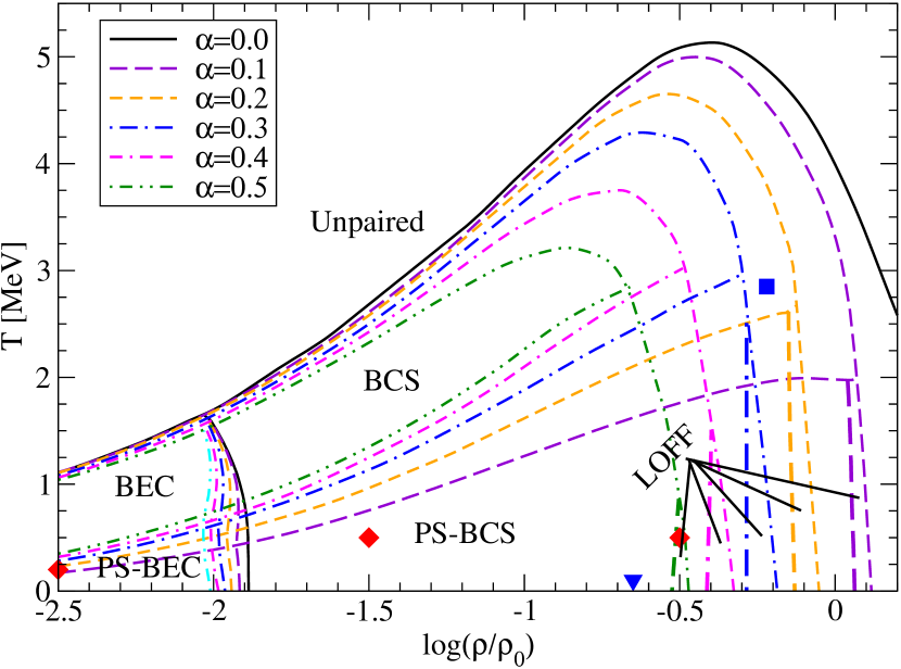
Figure 1.2: Phase diagram of dilute nuclear matter in the temperature-density plane for several isospin asymmetries $\alpha$ (from [18]). Included are four phases: unpaired phase, BCS (BEC) phase, LOFF phase, and PS-BCS (PS-BEC) phase. For each asymmetry between $0<\alpha<\alpha_{\mathrm{LOFF}}$ there are two tri-critical points, one of which is always a Lifshitz point [63]. For special values of asymmetry these two points degenerate into a single tetra-critical point for $\log(\rho_{4}/\rho_{0})=-0.22$, $T_{4}=2.85$ MeV and $\alpha_{4}=0.255$ (shown by a square). The LOFF phase disappears at the point $\log(\rho_{\mathrm{LOFF}}/\rho_{0})=-0.65$, $\alpha_{\mathrm{LOFF}}=0.62$ and $T=0$ (shown by a triangle). The boundaries between BCS and BEC phases are identified by the change of sign of the average chemical potential $\bar{\mu}$. The red diamonds refer to three regions of the phase diagram explained later.

The phase diagram has a richer structure at non-zero isospin, as can be seen in Fig. 1.2 where the phase structure is shown for several values of isospin asymmetry $\alpha=(\rho_{n}-\rho_{p})/(\rho_{n}+\rho_{p})$, where $\rho_{n}$ and $\rho_{p}$ are the number densities of neutrons and protons and $\rho_{0}=0.16\,\mathrm{fm}^{-3}$ is the nuclear saturation density. There are four different phases of matter in the phase diagram (see Eq. (1.56)), which we discuss in turn:

(a) The unpaired normal phase, which is the ground state for temperatures $T>T_{c}(\rho,\alpha)$, where $T_{c}(\rho,\alpha)$ is the critical temperature of the superfluid phase transition for any given asymmetry.

(b) The LOFF phase is the ground state for nonvanishing values of $\alpha$ within the range $0<\alpha<\alpha_{\mathrm{LOFF}}$ and high densities with $\rho>\rho_{\mathrm{LOFF}}$ and in a narrow temperature-density strip at low temperatures with $T<T_{4}$. Here $\alpha_{\mathrm{LOFF}}$ and $\rho_{\mathrm{LOFF}}$ correspond to the point of maximal asymmetry and at the same time the minimal density were the LOFF phase exists at $T=0$. This is shown by a blue triangle in Fig. 1.2. $\rho_{4}$, $T_{4}$ and $\alpha_{4}$ belong to the tetra-critical point, where the four phases BCS, PS-BCS, LOFF and unpaired phase coexist. This is shown by a blue square in Fig. 1.2. As borders for the LOFF phase we have the triangle with $\log(\rho_{\mathrm{LOFF}}/\rho_{0})=-0.65$, $T=0$ and $\alpha_{\mathrm{LOFF}}=0.62$ and the square with $\log(\rho_{4}/\rho_{0})=-0.22$, $T_{4}=2.85$ MeV and $\alpha_{4}=0.255$.

(c) For nonvanishing asymmetry, the phase-separated (PS) phase is the ground state for low temperatures and densities.

(d) The isospin-asymmetric BCS phase is the ground state at intermediate temperatures below the transition to the unpaired phase and above the transition to the PS phase and densities above the crossover to a BEC.

One may, of course, pose the question of the structure of the phase diagram in the high-density limit. At sufficiently large density, when the chemical potentials of nucleons become of the order of the rest mass of hyperons, the matter may become hyperon rich. This may occur at about twice the nuclear saturation density. Furthermore, at very high densities the interparticle distances decrease to values smaller than the nucleon radius and the quarks bound in nucleons may deconfine into free quarks.

The phase transitions have a very interesting shape. In addition to the crossover lines, we see several phase transition lines, resulting in two tri-critical points, where three phases coexist. At asymmetries below $\alpha_{4}$, we have a low-density tri-critical point, where the PS-BCS, the LOFF and the BCS phase coexist and a high-density tri-critical point, where the LOFF, the BCS and the unpaired phase coexist. However, at asymmetries above $\alpha_{4}$, we obtain a low-density tri-critical point with PS-BCS, BCS and unpaired phase and a high-density tri-critical point with PS-BCS, LOFF and unpaired phase. Interestingly they degenerate into a tetra-critical point, where PS-BCS, BCS, LOFF and unpaired phase coexist at asymmetry $\alpha_{4}$.

To access the order of various phase transitions (first or second order) we examine the behavior of the gap function across the phase diagram. This is illustrated in Fig. 1.3. In the upper panel we present the gap at fixed temperature and asymmetry for increasing density for three different phases. The calculated gap for the LOFF phase does not take into account the possibility of a PS-phase and vice versa. The BCS gap calculation ignores the possibility of the LOFF and PS pairing. Of course, the phase realized in nature is the one with the lowest free energy. In the lower panel we present the LOFF momentum ${\bm{Q}}$ and the PS filling fraction $x$ with a reference to the corresponding gaps presented in the upper panel. At low densities ${\bm{Q}}=0$ and $x=0$ and the BCS phase is the ground state. With increasing density we find $x\neq 0$, therefore a phase transition into the PS-BCS phase occurs which breaks the homogeneity of the system. If we ignore the possibility of the PS phase, a phase transition to the LOFF phase at higher density occurs; this breaks the translational symmetry. Since both, the filling parameter ($x$) of the PS phase and the momentum of the condensate (${\bm{Q}}$) of the LOFF phase increase smoothly, the change in the gap is also smooth and the phase transitions are second order. If we increase the density, ignoring the possibility of a PS or LOFF phase, the BCS gap vanishes smoothly. The same holds for the gap of the LOFF phase, if we consider the possibility of the LOFF phase but ignore the possibility of the PS phase. If we consider the PS phase but ignore the possibility of a LOFF phase, the filling fraction $x$ increases smoothly and we obtain a second order phase transition from BCS, PS-BCS or LOFF to the unpaired phase. The same holds for phase transitions from BEC, BCS, PS-BCS or LOFF to the unpaired phase with increasing temperature. However, if we take PS-BCS and LOFF phases into account, the free energy of the LOFF phase becomes less than the free energy of the PS-BCS phase at a certain density. At this point the gap does not change smoothly and therefore a first order phase transition is expected. To summarize, we have second order phase transitions from all superfluid phases to the unpaired phase and between superfluid phases, with the exception of a first order phase transition between the PS-BCS and LOFF phase (thick lines in Fig. 1.2). The transitions from BCS to BEC and from PS-BCS to PS-BEC are smooth crossovers.

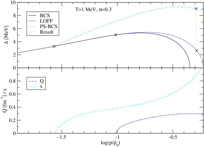
Figure 1.3: Upper panel: The gap of various phases. Lower panel: LOFF momentum ${\bm{Q}}$ and PS filling fraction $x$.

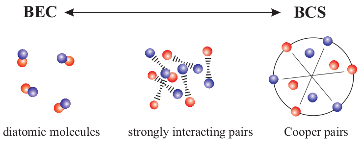
Figure 1.4: An illustration of the crossover from [36]. On the left we see bound deuterons, on the right we see unbound Cooper-pairs.

As mentioned above the low density limit of the phase diagram corresponds to the strong-coupling limit where a BEC of deuterons emerges. At intermediate temperatures we find a direct crossover from the ordinary BCS phase to a BEC consisting of bound deuterons and free neutrons. The situation is more complicated at low temperatures. The crossover occurs in the presence of the PS phase. Therefore, we obtain a crossover from the PS-BCS (which features a mixture of symmetric BCS and an asymmetric unpaired phase) to the PS-BEC phase where the symmetric BCS domains are replaced by a symmetric BEC of deuterons. These transformations are not phase transitions, but smooth crossovers, since no symmetry is broken. Therefore, the points of the phase diagram where BCS, BEC and unpaired phases coexist cannot be viewed as critical points. The same applies to the points where BCS, BEC, PS-BCS, PS-BEC coexist.

In the BCS limit, the size of a Cooper-pair is given by the coherence length $\xi$ which is very large compared to the average interparticle distance $d$. In the BEC limit the pairs are tightly bound deuterons with $\xi\ll d$. This is illustrated schematically in Fig. 1.4. Fig. 1.5 zooms in at the crossover region of Fig. 1.2 and shows the results including and excluding the PS phase. At higher temperatures the PS phase does not arise and we observe an ordinary BCS-BEC crossover even in the presence of isospin asymmetry. However, note that at sufficiently low temperatures, the crossover density decreases with decreasing temperature. At constant density the interparticle distance $d$ does not change. By decreasing the temperature we have two competitive effects affecting each other. At lower temperatures the particles have less momentum and thus pairing can occur at lower distances, which means that $\xi$ decreases and the crossover is shifted to higher densities. However, by increasing asymmetry we have less protons and thus less pairs, therefore $\xi$ increases, which means, that the crossover is shifted to lower densities. At high temperatures, the temperature can smear out the Fermi edges and thus the asymmetry effect is weak. However, at low temperatures the temperature induced smearing is weak compared to the asymmetry effect. Thus, the effect induced by asymmetry dominates at low temperatures and high asymmetries. Taking the PS-phase into account, we see that the crossover density increases with decreasing temperature for temperatures below the phase transition from BCS/BEC to PS-BCS/PS-BEC. In the PS phase, we have an isospin symmetric BCS/BEC domain in the matter. This means that $\xi$ is lower than in the ordinary BCS/BEC phase and thus the crossover is shifted to higher densities towards the $\alpha=0$ result.

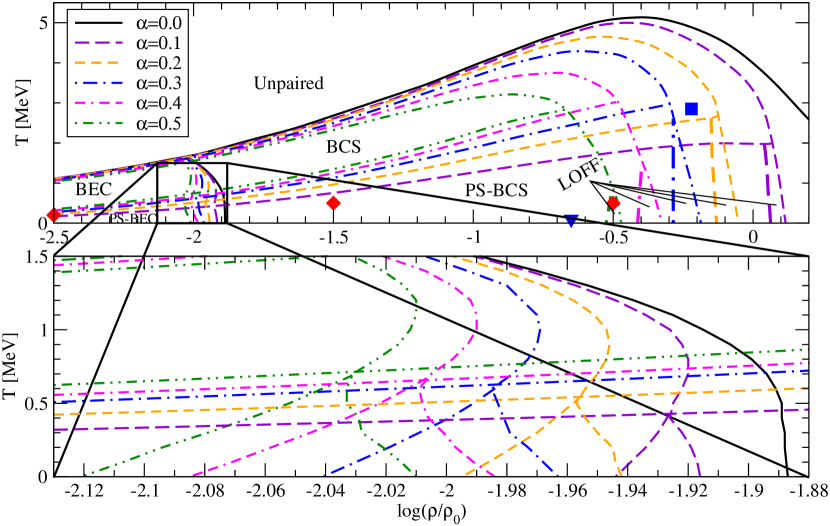
Figure 1.5: The upper panel shows the complete phase diagram, as seen in Fig. 1.2. The lower panel zooms in the crossover region. The horizontal lines here show the phase transition lines for different asymmetries between the BCS/BEC phase (which exists above a given asymmetry line) to the PS phase (which exists below the line). The nearly vertical lines show the crossover from BCS to BEC regimes. The left line is the case without PS phase, whereas the right line is the one including the PS phase. Thus, the inclusion of the PS phase induces the BCS-BEC crossover at higher density.

In the following we will discuss the crossover in detail. For that purpose we choose three points (marked with red diamonds in Fig. 1.2) which correspond to the weak, strong and intermediate couplings. Indeed, the point at $\log(\rho/\rho_{0})=-0.5$ and $T=0.5$ MeV corresponds to the high-density weak-coupling region (WCR) where we clearly have BCS pairing. For the low-density strong-coupling region (SCR) we choose the parameter values $\log(\rho/\rho_{0})=-2.5$ and $T=0.2$ MeV as representative for the BEC pairing. For comparison we also choose one point in between in the intermediate-coupling region (ICR) at $\log(\rho/\rho_{0})=-1.5$ and $T=0.5$ MeV. We have chosen low values for the temperatures to make sure that the matter is in all cases in the well developed condensate phase.

1.3.2 Temperature and asymmetry dependence of the gap: contrasting the BCS and LOFF phases

We now turn to the discussion of the properties of individual phases appearing in our phase diagram focusing on the key features. As a first step in understanding the mechanism that governs the appearance of various phases at different regimes present in the phase diagram we now focus on the behavior of the gap function as a function of temperature and asymmetry at constant density. We concentrate only on the weak-coupling regime (WCR), as the behavior of the gap function in the strong coupling regime (SCR) is self-similar to that of the WCR. For now, we also neglect the possibility that the PS phase is the ground state. Fig. 1.7 shows the weak-coupling gap as a function of temperature for a range of asymmetries. The plotted results for each nonzero value of $\alpha$ reveal different regimes of relatively low and relatively high temperature that reflect the different behaviors of the gap when the possibility of a LOFF phase is taken into account (solid curves) and when it is not (dashed curves). Two branches existing at lower temperatures merge at some point to form a single segment stretching up to the critical temperature of phase transition. This high-temperature segment corresponds to the BCS state, and the temperature dependence of the gap is standard, with $d\Delta(T)/dT<0$ and asymptotic behavior $\Delta(\alpha,T)\sim[T_{c}(\alpha)(T_{c}(\alpha)-T)]^{1/2}$ as $T\to T_{c}(\alpha)$, where $T_{c}(\alpha)$ is the (upper) critical temperature. In the low-temperature region below the branching point, there are two competing phases (BCS and LOFF), with very different temperature dependences of the gap function. The quenching of the BCS gap (dashed lines) as the temperature is decreased is caused by the loss of coherence among the quasiparticles as the thermal smearing of the Fermi surfaces disappears.

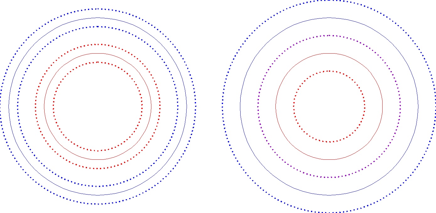
Figure 1.6: The proton Fermi surface is shown by a red solid line, the neutron Fermi surface is shown by a blue solid line. The dotted lines present the temperature induce smearing. The temperature in the right figure is bigger than in the left one.

Consequently, in the low-temperature range below the branch point, the BCS branch shows the unorthodox behavior $d\Delta(T)/dT>0$, and for large enough asymmetries there exists a lower critical temperature $T_{c}^{*}$ [22].

This effect is illustrate in Fig. 1.6, where the Fermi-spheres of protons and neutrons are shown by red and blue solid lines, respectively. The dotted concentric circles illustrate the smearing induced by temperature. For pairing we need an overlap of the Fermi spheres, thus the smearing of the temperature needs to overcome the shift of the Fermi levels due to asymmetry. In the left plot the smearing of the temperature is too low and coherence is lost. On the right it is large enough to create an overlap. This simple picture captures the effect of temperature on the pairing in asymmetric systems: if temperature is high enough it restores the pairing correlations which are otherwise suppressed by the asymmetry.

On the contrary, one finds $d\Delta(T)/dT<0$ for the LOFF branch, as is the case in ordinary (symmetrical) BCS theory [64]. It should be mentioned that the “anomalous” behavior of the BCS gap below the point of bifurcation leading to the LOFF state gives rise to a number of anomalies in thermodynamic quantities, such as negative superfluid density or excess entropy of the superfluid [65]. These anomalies are absent in the LOFF state [66]. Fig. 1.8 shows the dependence of the gap function on asymmetry for several pertinent temperatures. In accord with Fig. 1.7, there are two curves (or segments) for each temperature: one in the low-$\alpha$ domain where only the BCS phase exists and the other in the large-$\alpha$ domain where both BCS (dashed lines) and LOFF states (solid lines) are possible. Clearly the LOFF solution, for which the gap extends to larger $\alpha$ values, is favored in the latter domain.

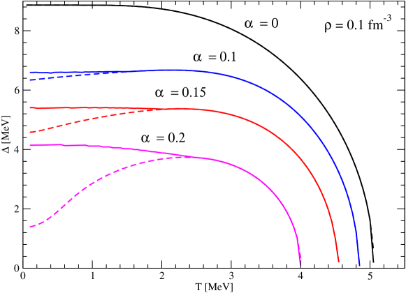
Figure 1.7: The gap as a function of the temperature at constant density $\rho=0.1$ fm^-3 for several asymmetries. Solid lines allow for the emergence of the LOFF phase, whereas the dashed lines show only the BCS phase.

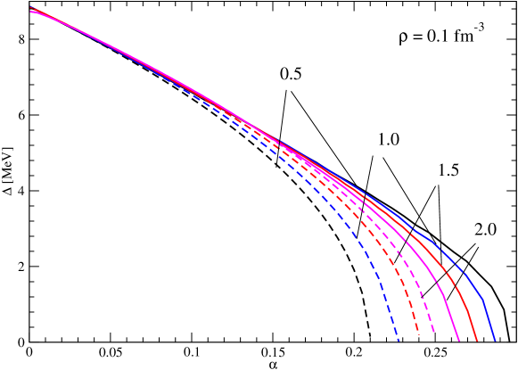
Figure 1.8: The gap as a function of the asymmetry at constant density $\rho=0.1$ fm^-3 for several temperatures, given in MeV. Solid lines allow for the emergence of the LOFF phase, whereas the dashed lines show only the BCS phase.

For small $\alpha$ the gap function is linear in $\alpha$. At the other extreme of large $\alpha$, the gap has the asymptotic behavior $\Delta(\alpha)\sim\Delta_{00}\left(1-\alpha/\alpha_{1}\right)^{1/2}$, where $\alpha_{1}\sim\Delta_{00}/\bar{\mu}$ and $\Delta_{00}$ is the value of the gap at vanishing temperature and asymmetry. The critical asymmetry $\alpha_{2}$ at which the LOFF phase transforms into the normal phase is a decreasing function of temperature, whereas that for termination of the BCS phase (denoted $\alpha_{1}$ above) increases up to the temperature where $\alpha_{1}=\alpha_{2}$. For higher temperatures, $\alpha_{1}$ decreases with temperature. Consequently, in the dominant phase the critical asymmetry always decreases with temperature.

1.3.3 Occupation numbers and chemical potentials

Next let us examine the behavior of the occupation numbers, which are defined as integrands of the densities appearing in Eq. 1.44, i.e.,

$$n_{n/p}({\bm{Q}}) = \left(1+\frac{E_{S}}{\sqrt{E_{S}^{2}+\Delta^{2}}}\right)f(E^{+}_{\mp})$$ (1.59)

$$+\left(1-\frac{E_{S}}{\sqrt{E_{S}^{2}+\Delta^{2}}}\right)(1-f(E^{-}_{\pm}))\,.$$

Fig. 1.9 shows the occupation numbers of neutrons and protons respectively for a fixed density of $\rho=0.04\,\mathrm{fm}^{-3}$ and a fixed asymmetry of $\alpha=0.3$ for several values of the temperature (see also the discussion in Subsec. 1.3.7). Due to the asymmetry, the Fermi surfaces are shifted by $\delta\mu$. Because $\rho_{n/p}=(1\pm\alpha)/2\cdot\rho$ and $k_{F}\propto\sqrt[3]{\rho}$, one can define new Fermi surfaces for neutrons and protons as $k_{F_{n/p}}/k_{F}=\sqrt[3]{1\pm\alpha}$, where $k_{F_{n/p}}$ are the Fermi momenta for neutrons and protons and $k_{F}$ is the Fermi momentum in isospin symmetric nuclear matter. The Fermi surfaces of neutrons and protons are presented by vertical black solid lines in Fig. 1.9. The prominent feature is the depletion of the proton occupation numbers around the common Fermi surface, which is most pronounced at low temperatures. At finite temperature this depletion is gradually washed out. Note that at the neutron Fermi surface, the proton occupancy increases again and these protons contribute most to the Cooper pairing with the neutrons at their Fermi surface. We thus have a Fermi distribution type occupation for protons and neutrons for $k\lesssim k_{{F_{p}}}$ and $k\gtrsim k_{{F_{n}}}$ respectively with a “breach” in the momentum range $k_{{F_{p}}}\lesssim k\lesssim k_{{F_{n}}}$. The effect of the temperature smearing is demonstrated illustratively in Fig. 1.6.

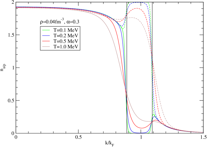
Figure 1.9: The neutron (proton) occupation numbers in the BCS phase are shown with dashed (solid) lines at a fixed density of $\rho=0.04\,\mathrm{fm}^{-3}$ and a fixed asymmetry of $\alpha=0.3$. The labeling of temperatures is shown in the plot with various colors. The vertical black solid lines present the Fermi momenta of neutrons and protons, respectively.

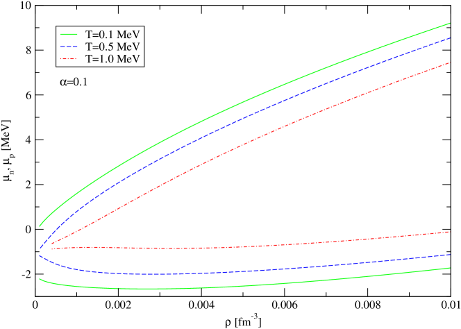
Figure 1.10: Chemical potentials of neutrons and protons in the BCS/BEC phase as a function of the density at $\alpha=0.1$ for several temperatures.

Fig. 1.10 shows the chemical potentials of protons and neutrons as a function of density for a fixed asymmetry of $\alpha=0.1$ for several values of the temperature. We see that the separation of proton and neutron chemical potentials decreases with decreasing density and with increasing temperature. In both cases the distributions of neutrons and protons are smeared out, Pauli blocking is less effective and the difference of the chemical potentials is also smeared out.

1.3.4 Effects of finite momentum in the LOFF phase

A phase-space overlap between the members of a Cooper-pair is required for pairing. Increasing the asymmetry shifts the Fermi momenta of neutrons and protons apart. BCS pairing at finite asymmetry thus requires smearing out of Fermi surfaces, which then provides the needed phase-space overlap. The overlap is large at high temperatures and low densities. Similar effect of restoration of phase-space overlap can be achieved if a total Cooper-pair momentum ${\bm{Q}}$ is allowed, as is the case in the LOFF phase. The shift of the Fermi-surfaces due to finite ${\bm{Q}}$ which restores pairing correlations in the limit of high densities, low temperatures and large asymmetries, is illustrated in Fig. 1.11.

Figure 1.11: The purpose of this figure is to illustrate the mechanism of phase-space restoration by the LOFF phase. The centers of the neutron and proton Fermi surfaces are shifted by ${\bm{Q}}$. The neutron and proton Fermi surfaces are shown by a blue or red cycle, respectively. We show the momenta of neutrons and protons for $\theta=45\degree$ which are constructed according to ${\bm{k}}_{n}={\bm{k}}_{F}+{\bm{Q}}/2$ and ${\bm{k}}_{p}={\bm{k}}_{F}-{\bm{Q}}/2$. These are drawn towards a point where the Fermi surfaces intersect and there is a maximal phase space overlap.

Fig. 1.11 illustrates the mechanism of phase-space restoration by the LOFF phase. In the case of high densities, low temperatures and finite asymmetry, pairing with finite ${\bm{Q}}$ is energetically favorable, because the negative pairing energy compensates the positive kinetic energy of motion of Cooper-pairs. The momenta of protons are shown in red and the ones of neutrons in blue. The Cooper-pair momentum ${\bm{Q}}$ describes the shift of the centers of the Fermi spheres. The relative momentum of the pairs at the Fermi surface ${\bm{k}}_{F}$ is shown for the angle $45\degree$. The corresponding neutron momentum is then given as ${\bm{k}}_{F}+{\bm{Q}}/2$ (in blue) and that of the proton is given by ${\bm{k}}_{F}-{\bm{Q}}/2$ (in red). By construction the sum of the momenta is such that $({\bm{k}}_{F}+{\bm{Q}}/2)+(-{\bm{k}}_{F}+{\bm{Q}}/2)={\bm{Q}}$. Note that we show the case where the Fermi-surfaces intersect and the overlap is optimal for pairing.

Fig. 1.12 shows the gap and the free energy for several densities, temperatures and asymmetries. We see that the maximum of the gap and the minimum of the free energy are at finite values of ${\bm{Q}}$ at high density, high asymmetry or low temperature. In particular, the gap at vanishing ${\bm{Q}}$ vanishes for high asymmetry or high density. At high temperatures, low asymmetries or low densities, we expect the translational symmetric BCS phase to be favored over the LOFF phase. By introducing the effective chemical potential $\tilde{\bar{\mu}}=(\bar{\mu}-Q^{2}/8m^{*})$ we obtain

$$E_{S} = k^{2}/2m^{*}-\tilde{\bar{\mu}}.$$ (1.60)

Thus, the non-zero total momentum implies that the average chemical potential of the BCS phase $\bar{\mu}$ is reduced.

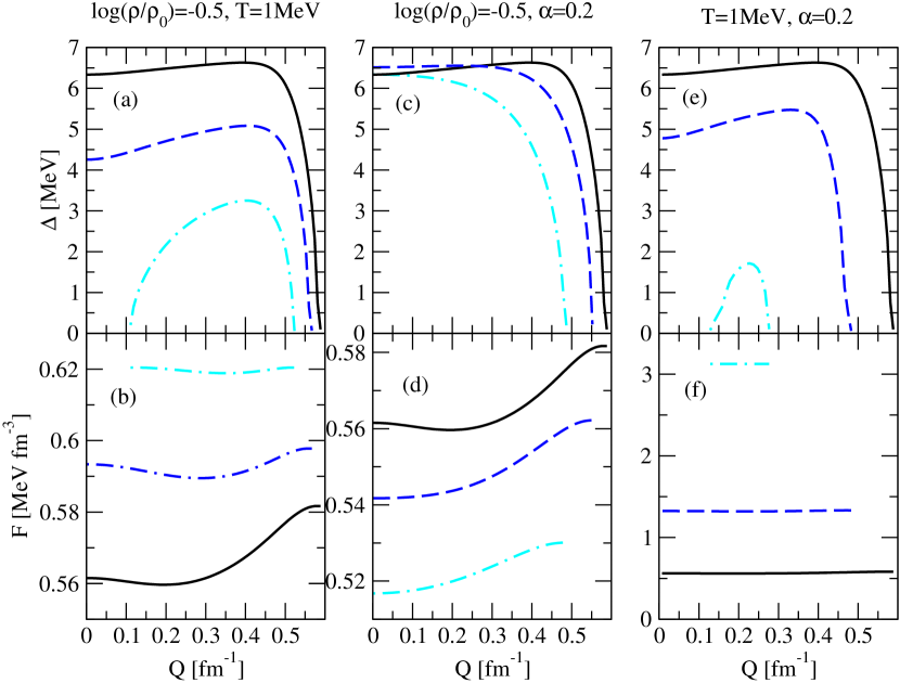
Figure 1.12: Properties of the nuclear LOFF phase. The upper panel shows the pairing gaps and the lower panel shows the free energies as a function of the total momentum ${\bm{Q}}$ of a Cooper-pair.
In (a) and (b) the density is fixed at $\log(\rho/\rho_{0})=-0.5$ and the temperature is fixed at $T=1$ MeV, the asymmetries are:
$\left.\right.\qquad\alpha=0.2$ (black, solid),
$\left.\right.\qquad\alpha=0.3$ (blue, dashed) and
$\left.\right.\qquad\alpha=0.4$ (cyan, dash-dotted).
In (c) and (d) the density is fixed at $\log(\rho/\rho_{0})=-0.5$, the asymmetry is fixed at $\alpha=0.2$, the temperatures are:
      1 MeV (black, solid),
      2 MeV (blue, dashed) and
      3 MeV (cyan, dash-dotted).
In (e) and (f) the temperature is fixed at $T=1$ MeV, the asymmetry is fixed at $\alpha=0.2$, the densities are:
$\left.\right.\qquad\log(\rho/\rho_{0})=-0.5$ (black, solid),
$\left.\right.\qquad\log(\rho/\rho_{0})=-0.3$ (blue, dashed) and
$\left.\right.\qquad\log(\rho/\rho_{0})=-0.1$ (cyan, dash-dotted).

1.3.5 The kernel of the gap equation

We start our study of the intrinsic quantities with the kernel of the gap equation,

$$K(k,\theta) \equiv \sum_{a,r}\frac{P^{a}_{r}}{4\sqrt{E_{S}^{2}(k)+\Delta^{2}(k,Q)}}.$$ (1.61)

This kernel is proportional to the imaginary part of the retarded anomalous propagator and the Pauli operator represented by $P_{r}^{a}=1-2f(E^{a}_{r})$. Physically, $K(k)$ can be interpreted as the wave function of the Cooper-pairs, since it obeys a Schrödinger-type eigenvalue equation in the limit of extremely strong coupling. The Pauli operator is a smooth function of the momentum having a minimum at the Fermi surface, where $E_{S}$ vanishes in the limit of weak-coupling. In Figs. 1.13-1.17 we present the kernel for several values of density, temperature and asymmetry as a function of the momentum. When studying the variation with density, temperature or asymmetry we fix the remaining quantities at the following values $\rho=0.04$ fm^-3, $T=0.2$ MeV, and $\alpha=0.3$. These values correspond to the BCS region in all figures where the density is fixed. The ranges of momenta which contribute substantially to the gap equation in different regimes of the phase diagram can be identified from these figures. We now discuss the insights that can be gained from these figures in some detail.

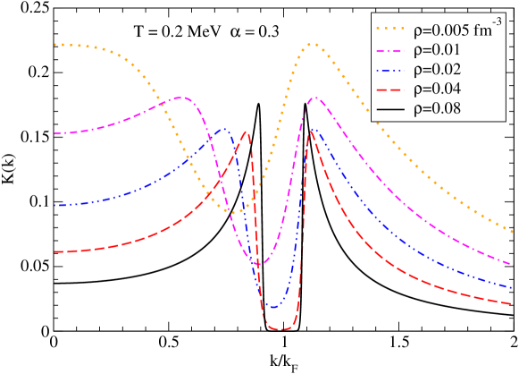
Figure 1.13: Dependence of the kernel $K(k)$ on momentum in units of Fermi momentum for fixed $T=0.2$ MeV, $\alpha=0.3$, and various densities indicated in the plot.

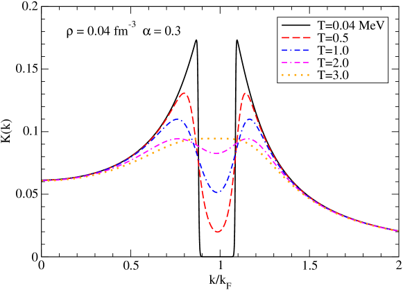
Figure 1.14: Dependence of the kernel $K(k)$ on momentum in units of Fermi momentum for fixed $\rho=0.04$ fm^-3, $\alpha=0.3$, and various temperatures indicated in the plot.

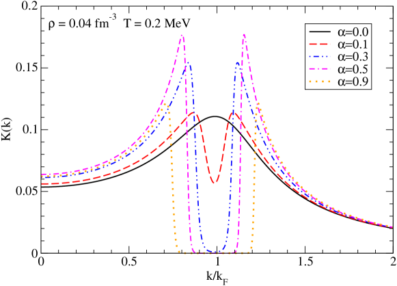
Figure 1.15: Dependence of the kernel $K(k)$ on momentum in units of Fermi momentum for fixed $\rho=0.04$ fm^-3, $T=0.2$ MeV, and various values of asymmetry indicated in the plot.

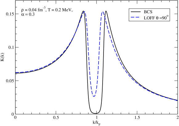
Figure 1.16: Dependence of the kernel $K(k)$ on momentum in units of Fermi momentum at fixed $\rho=0.04$ fm^-3, $T=0.2$ MeV, and $\alpha=0.3$ for the BCS phase and the LOFF phase at $\theta=90\degree$, where $\theta$ is the angle formed by the CM and relative momenta in Eq. (1.61).

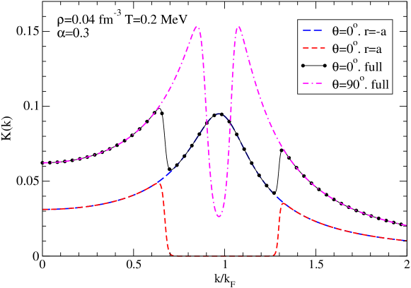
Figure 1.17: Dependence of the kernel $K(k)$ on momentum in units of Fermi momentum at fixed $\rho=0.04$ fm^-3, $T=0.2$ MeV, and $\alpha=0.3$ for the LOFF phase, where $\theta$ is the angle formed by the CM and relative momenta in Eq. (1.61). In the case $\theta=0\degree$ the full result (black, solid-filled-circle line) is decomposed into components with $r=-a$ (blue, long dashed line) and $r=a$ (red, short dashed line).

Fig. 1.13 shows the function $K(k)$ at constant temperature and asymmetry for various densities. The high densities correspond to the BCS regime, and the low densities to the BEC regime, allowing us to follow the evolution of this function through the BCS-BEC crossover. In the BCS regime, $K(k)$ has two sharp maxima which are separated by a depression of width ∼ $\delta\mu$ around the Fermi momentum. The lower maximum is located at the Fermi momentum of protons, whereas the upper maximum at the Fermi momentum of neutrons. As discussed in Subsec. 1.3.7 below, this feature originates from the Pauli operator. Because of their strong localization in momentum space, the Cooper-pairs have an intrinsic structure that is broad in real space, implying a large coherence length. This is characteristic of the BCS regime. The picture is reversed in the strong-coupling (low-density) limit, where $K(k)$ is a broad function of momentum, corresponding to the presence of bound states (deuterons), which are well-localized in real space. This is characteristic of the BEC regime. In addition, as the density decreases, the lower (proton) peak moves toward $k=0$ and also the minimum moves away from $k=k_{F}$ towards lower momenta, due to the fact that $\bar{\mu}$ changes its sign from positive to negative at the transition from the BCS to the BEC regime. As a consequence, the prefactor of the Pauli operator $P^{r}_{a}$ peaks at $k=0$ in the BEC regime, rather than at the Fermi surface as in the BCS regime. In addition, one can clearly see a smearing of the two peaks of the kernel with decreasing density.

Fig. 1.14 shows the function $K(k)$ for various temperatures, now at constant asymmetry and constant density, such that the system is situated in the BCS regime. At low temperatures, $K(k)$ is seen to have two maxima separated by a depression around the Fermi momentum, as already discussed above. Increasing the temperature smears out the structures characteristic of the low-temperature case, due to temperature-induced blurring of the Fermi surface. Close to $T_{c}$, the temperature effects dominate over the effects of asymmetry. Consequently, the double-peak structure disappears and the isospin asymmetry does not affect the properties of the condensate.

Fig. 1.15 shows the function $K(k)$ for various asymmetries at constant temperature and the same density as above (thus again implying the BCS regime). We can now follow how the double peak-structure builds up as the asymmetry is increased. Because the width of the depression is proportional to $\delta\mu$, it increases with increasing isospin asymmetry, a behavior consistent with the facts that the Fermi surfaces of neutrons and protons are pulled apart by the isospin asymmetry, and that in the BCS regime the available phase space is constrained to the vicinity of the corresponding Fermi surface. (See also the Subsec. 1.3.3 for a discussion of the Fermi momenta.)

Finally, in Figs. 1.16 and 1.17 we show $K(k)$ for fixed values of temperature, asymmetry, and density, in Fig. 1.16 for the BCS phase and the LOFF phase at $\theta=90\degree$ and in Fig. 1.17 for the LOFF phase at two values of the angle formed by the relative and CM momenta, as defined in Eq. (1.61). It is seen from Fig. 1.16 that in the orthogonal case ($\theta=90\degree$) the double-peak structure present in the BCS phase remains, although the effects of asymmetry are weaker compared to the BCS case. This is easily understood by noting that $E_{A}=0$ for $\theta=90\degree$, therefore finite momentum induces only a shift in the energy origin according to $\bar{\mu}\to\bar{\mu}-Q^{2}/8m^{*}$. The case $\theta=0\degree$ in Fig. 1.17 exposes an interesting feature of the LOFF phase: for a range of orientations of the CM momentum of Cooper-pairs ($\theta\approx 0\degree$), the effects of asymmetry are mitigated and the kernel obtains a maximum at $k/k_{F}=1$, which is a combination of the contribution from $r=-a$ which acts to enhance the pairing correlations in the vicinity of the Fermi surface and the $r=a$ contribution which vanishes in this region.

1.3.6 The Cooper-pair wave function across the BCS-BEC crossover

The transition to the BEC regime of strongly-coupled neutron-proton pairs, which are asymptotically identical with deuterons, occurs at low densities. The criterion for the transition from BCS to BEC is that either the average chemical potential $\bar{\mu}$ changes its sign from positive to negative values, or the coherence length $\xi$ of a Cooper-pair becomes comparable to the interparticle distance, i.e., $\xi$ becomes of order $d\sim\rho^{-1/3}$. (In the BCS regime $\xi\gg d$, whereas in the BEC regime $\xi\ll d$).

The coherence length can be related to the root-mean-square of the Cooper-pair wave function, as we show below. The wave function of a Cooper-pair is defined in terms of the kernel of the gap equation according to

$$\Psi(\bm{r})=\sqrt{N}\int\frac{d^{3}p}{(2\pi)^{3}}[K({\bm{p}},\Delta)-K({\bm{p}},0)]e^{i{\bm{p}}\cdot\bm{r}}\,,$$ (1.62)

which, after integration over angles, becomes

$$\Psi(r) = \frac{\sqrt{N}}{2\pi^{2}r}\int_{0}^{\infty}dp\,p\,[K(p,\Delta)-K(p,0)]\sin(pr)\,,$$ (1.63)

where $N$ is a constant determined by the normalization condition

$$N\int d^{3}r|\Psi(\bm{r})|^{2}=1\,.$$ (1.64)

In Eq. (1.62) we subtract from the kernel its value $K({\bm{p}},0)$ in the normal state to regularize the integral, which is otherwise divergent. Cut-off regularization of this strongly oscillating integral is not appropriate. The mean-square radius of a Cooper-pair is defined via the second moment of the probability density,

$$\langle r^{2}\rangle=\int d^{3}r\,r^{2}|\Psi(\bm{r})|^{2}\,.$$ (1.65)

The coherence length, i.e., the spatial extension of a Cooper-pair, is then defined as

$$\xi_{\rm rms}=\sqrt{\langle r^{2}\rangle}\,.$$ (1.66)

Thus the change in the coherence length is related to the change of the condensate wave function across the BCS-BEC crossover. The regimes of strong and weak coupling can be identified by comparing the coherence length to the mean interparticle distance $d=(3/(4\pi\rho))^{1/3}$. In the BCS regime the coherence length is given by the well-known analytical formula

$$\xi_{a}=\frac{\hbar^{2}k_{F}}{\pi m^{*}\Delta}\,.$$ (1.67)

Table 1.1 lists the analytical and root-mean-square values of the coherence length for several densities and temperatures, chosen to represent the different regimes WCR, ICR, and SCR, together with the corresponding values of the mean interparticle distance. It is seen that in the case of neutron-proton pairing, one of the criteria for the BCS-BEC transition is fulfilled, namely, the mean distance between the pairs becomes larger than the coherence length of the superfluid as one goes from WCR to SCR for the numerical computed coherence length $\xi_{\mathrm{rms}}$. This is not the case for the analytical expression $\xi_{a}$. Thus one should rely only on the numerical value $\xi_{\mathrm{rms}}$. We have verified that the average chemical potential changes its sign accordingly, so that the second criterion is fulfilled as well.

	log$\left(\frac{\rho}{\rho_{0}}\right)$	$k_{F}$[fm-1]	$T$ [MeV]	$d$ [fm]	$\xi_{\rm rms}$ [fm]	$\xi_{a}$ [fm]
WCR	$-0.5$	0.91	0.5	1.68	3.17	1.41
ICR	$-1.5$	0.42	0.5	3.61	0.94	1.25
SCR	$-2.5$	0.20	0.2	7.79	0.57	1.79

Table 1.1: For each of the three regimes of coupling strength, corresponding values are presented for the density $\rho$ (in units of nuclear saturation density $\rho_{0}=0.16$ fm^-3), Fermi momentum $k_{F}$, temperature $T$, interparticle distance $d$, and coherence parameters $\xi_{\rm rms}$ and $\xi_{a}$. The values of the gap and effective mass (in units of bare mass) at $\alpha=0$ in these three regimes are 9.39, 4.50, 1.44 MeV and 0.903, 0.989, 0.999, respectively. In the WCR, the LOFF phase is found in the vicinity of asymmetry $\alpha=0.49$, for which $\Delta=1.27$ MeV and $Q=0.40$ fm^-1.

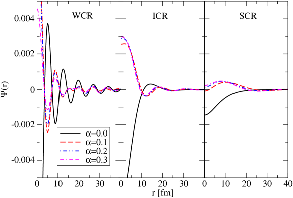
Figure 1.18: Dependence of $\Psi(r)$ on $r$ for the three coupling regimes and various values of asymmetry (see Table 1.1 for values of density and temperature).

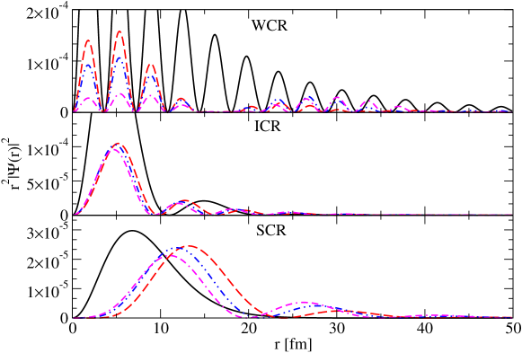
Figure 1.19: Dependence of $r^{2}|\Psi(r)|^{2}$ on $r$ for the three coupling regimes. Conventions are the same as in Fig. 1.18.

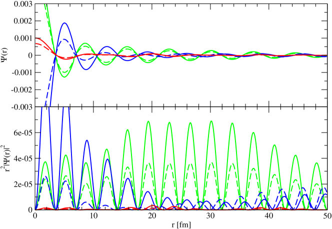
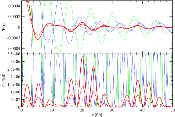
Figure 1.20: Dependence of $\Psi(r)$ and $r^{2}|\Psi(r)|^{2}$ on $r$ in the WCR for three different angles $\theta$: green $\theta=0\degree$, blue $\theta=45\degree$ and red $\theta=90\degree$ for two different asymmetries: solid lines for $\alpha=0.49$ and dashed lines for $\alpha=0.50$ at which the LOFF phase is the ground state. The figures only differ in the scale and show the results for $\theta=0\degree$ and $\theta=45\degree$ (top figure) and $\theta=90\degree$ (bottom figure).

Fig. 1.18 shows the wave function of Cooper-pairs as a function of radial distance across the BCS-BEC crossover for various densities. In weak coupling, the wave function has a well-defined oscillatory form that extends over many periods of the interparticle distance. Such a state conforms to the familiar BCS picture, in which the spatial correlations are characterized by scales that are much larger than the interparticle distance. We clearly see a decrease of the amplitude with increasing asymmetry, which is correlated with the observation that the asymmetry decreases the gap. For intermediate and strong coupling the wave function is increasingly concentrated at the origin with at most a few periods of oscillation. The strong-coupling limit corresponds to pairs that are well localized in space within a small radius. This regime clearly has BEC character, with the pair correlations extending only over distances comparable to the interparticle distance. At large distances the asymmetry does not change the shape of the wave function significantly. However, at small distances the changes are significant. In the SCR $\Psi(\bm{r})$ has, for vanishing asymmetry, a minimum at $r=0$ and reaches asymptotically $\Psi(\bm{r})=0$ for $r\rightarrow\infty$. Increasing the asymmetry increases the small-distance values leading to a maximum at nonvanishing $r$. The function $\Psi(\bm{r})$ in the ICR and at vanishing asymmetry starts at a large negative value and oscillates only once to a maximum. At nonvanishing asymmetry $\Psi(\bm{r})$ starts at a large positive value which is followed by oscillatory behavior. The first minimum at nonvanishing asymmetry is at lower $r$ than the first maximum at vanishing asymmetry. In the WCR we find a regularly oscillating shape at vanishing asymmetry with the amplitude vanishing for large $r$. For nonvanishing asymmetry we basically have two segments. In the large $r$ segment the symmetric and asymmetric condensate wave-functions oscillate in-phase. For small $r$ the oscillations are counter-phase. The transition between these segments is characterized by $\Psi(\bm{r})\approx 0$. As a general trend we find that the wave function is almost independent of the asymmetry in the WCR. In the SCR there are substantial changes as soon as asymmetry is switched on.

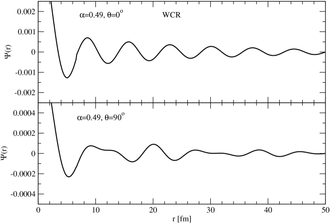
Figure 1.21: Dependence of $\Psi(r)$ on $r$ in the WCR for two different angles $\theta$ and for asymmetry $\alpha=0.49$ at which the LOFF phase is the ground state. (Cutout of Fig. 1.20)

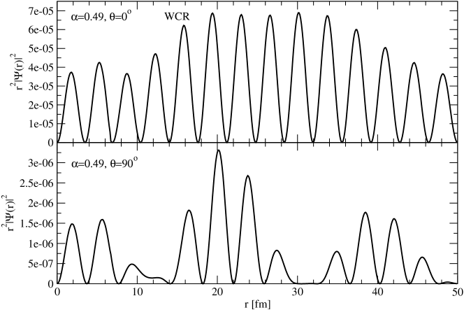
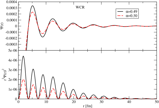
Figure 1.22: Dependence of $r^{2}|\Psi(r)|^{2}$ on $r$ in the WCR for two different angles $\theta$ and for asymmetry $\alpha=0.49$ at which the LOFF phase is the ground state. (Cutout of Fig. 1.20)

Figure 1.23: Dependence of $\Psi(r)$ and $r^{2}|\Psi(r)|^{2}$ on $r$ in the WCR integrated over the angle $\theta$ for asymmetries $\alpha=0.49$ and $\alpha=0.50$ at which the LOFF phase is the ground state.

Fig. 1.19, complementary to Fig. 1.18, displays the quantity $r^{2}|\Psi(\bm{r})|^{2}$. The spatial correlation in the SCR is dominated by a single peak corresponding to a tightly bound state close to the origin. The existence of residual oscillations indicates that there is no unique bound state formed at such coupling, but the tendency towards its formation is clearly seen. We find that in the weak coupling there is perfect match in the maxima of the function $r^{2}|\Psi(\bm{r})|^{2}$ for all asymmetries (which was less visible in Fig. 1.18 where the oscillations are counter-phase). An oscillatory structure appears in the ICR as a fingerprint of the transition from the BEC to the BCS regime. In this case there are similar changes of maxima and zeros, which is also the case in SCR. At low and high asymmetries the strong-coupling peaks are well defined, whereas at intermediate asymmetries the weight of the function is distributed among several peaks. By increasing the coupling from WCR via ICR to SCR we see a change of the shape from a heavily oscillating wave function of unbound Cooper-pairs fixed in momentum space and spread in real space in the WCR to a single peak dominated wave function of bound deuterons fixed in real space and spread in momentum space, pronounced best for $\alpha=0$.

Figs. 1.20 to 1.23 demonstrate the same quantities, i.e., $\Psi(\bm{r})$ and $r^{2}|\Psi(\bm{r})|^{2}$ for the case of the LOFF phase computed at the WCR point of the phase diagram (as specified in Table 1.1). In Fig. 1.20 a broad range of angles and asymmetries is shown, whereas Figs. 1.21 and 1.22 show only the essential features. Fig. 1.23 presents the angle integrated quantities. At this point the LOFF phase is the ground state of the matter at asymmetry $\alpha=0.49$ ($\delta\mu=6.45$ MeV), where $\Delta=1.27$ MeV and $Q=0.40$ fm^-1 and at $\alpha=0.50$ ($\delta\mu=6.51$ MeV), where $\Delta=0.84$ MeV and $Q=0.40$ fm^-1. For slightly lower asymmetries ($\alpha\leq 0.48$) the system is in the PS phase, whereas for $\alpha>0.50$ the gap is vanishingly small, the system being in the normal state. Unfortunately it is not possible to carry out a direct comparison between BCS and LOFF, since the gap of the BCS vanishes at $\alpha=0.37$ in the WCR. In the case $\theta=0\degree$ and $\theta=45\degree$ the perfect oscillatory behavior seen in $\Psi(\bm{r})$ in the BCS case is replicated, as in this case the finite momentum of the condensate does not contribute to the spectrum of the Cooper-pairs. This shape is also seen for the angle integrated result, because contributions of angles around $\theta\approx 0\degree$ are dominant. Regarding $r^{2}|\Psi(\bm{r})|^{2}$ at $\theta=0\degree$ we see that the maxima first increase in value with a maximum at about $r=25$ fm and afterwards decrease. This is due to the phase, which can be chosen freely. Thus the physics at $\theta=45\degree$ and $\theta=0\degree$ does not differ significantly. In the case $\theta=90\degree$ $\Psi(\bm{r})$ is distorted in the LOFF phase by the presence of a second oscillatory mode with the period $2\pi/Q$ in addition to the first mode, with the period $2\pi/k_{F}$. The additional periodic structure is more pronounced in the quantity $r^{2}|\Psi(\bm{r})|^{2}$, where the rapid oscillations are modulated with a period $\approx 16$ fm. Moreover we see a large decrease of the amplitude at $\theta=90\degree$ compared to $\theta\approx 0\degree$ because of the low phase-space overlap.

1.3.7 Occupation numbers across the BCS-BEC crossover

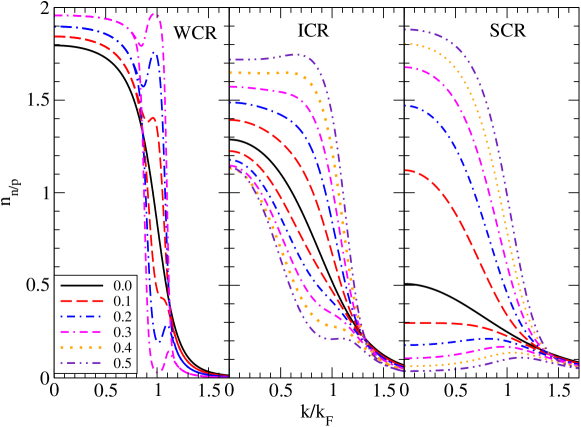
Figure 1.24: Dependence of the neutron and proton occupation numbers on momentum $k$ (in units of Fermi momentum) for the three coupling regimes and various asymmetries indicated in the legend.

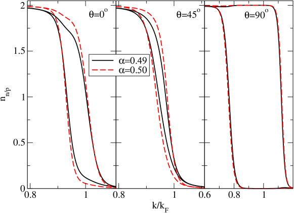
Figure 1.25: Dependence of the neutron and proton occupation numbers on momentum $k$ (in units of Fermi momentum) in the WCR for two asymmetries where the LOFF phase is the ground state. The three angles indicated refer to the neutron occupation numbers. The proton occupation numbers are plotted for angles $180\degree-\theta$. Note: For $\theta=0\degree$ the neutron curves are the left ones.

The integrand of Eq. (1.44) defines the occupation numbers $n_{n/p}(k)$ of the neutrons and protons, given by $n_{n/p}(k)=n_{n/p,\uparrow}(k)+n_{n/p,\downarrow}(k)$. The maximal value of $n_{n/p}(k)$ is therefore two. The Cooper-pairs with total momentum ${\bm{Q}}$ represent pairs with individual momenta ${\bm{k}}+{\bm{Q}}/2$ (neutrons) and $-{\bm{k}}+{\bm{Q}}/2$ (protons).

Regarding Eq. (1.44) and Eq. (1.37) we see that the energy shift due to the Cooper-pair momentum has the opposite direction of the energy shift due to the mismatch of the Fermi spheres and therefore promotes pairing for $\theta<90\degree$ in case of neutrons and $\theta>90\degree$ in case of protons. To achieve a better comparison, we therefore depict the proton occupation numbers at $180\degree-\theta$. These quantities are shown in different coupling regimes of the BCS-BEC crossover in Fig. 1.24. In the WCR (leftmost panel) the occupation numbers of protons exhibit a “breach” [67] or “blocking region” for large asymmetries, i.e., the minority component is entirely expelled from the blocking region ($n_{p}=0$), while the majority component is maximally occupied ($n_{n}/2=1$). In the small-$\alpha$ limit the occupation numbers are clearly fermionic (with some diffuseness due to the temperature), in that all single-particle states below a certain mode (the Fermi momentum at $T=0$) are almost filled, while all states above are nearly empty. We have verified that in the high-temperature limit the breach is filled in, the occupation numbers becoming smooth functions of momentum; consequently the low-momentum modes are less, this can be seen in Fig. 1.9. Since the densities of neutrons and protons are different, Fermi momenta are shifted to $k_{F_{n/p}}/k_{F}=\sqrt[3]{1\pm\alpha}$ as explained in Subsec. 1.3.3. For uncoupled particles, we would expect two independent Fermi distributions with different $k_{F_{n/p}}$ at finite asymmetry. However, we see a special behavior around the Fermi surface also explained in Subsec. 1.3.3.

In the ICR (middle panel) the fermionic nature of the occupation numbers is lost. The low-momentum modes are not fully populated and, accordingly, high-momentum modes are more heavily occupied. A Fermi surface cannot be identified because of the smooth population of the modes. Moreover, a breach no longer appears for the parameters chosen. It is also to be noted that for large asymmetries $\alpha\geq 0.4$, the momentum dependence of the occupation numbers becomes non-monotonic; for the minority component this is a precursor of the change in the topology of the Fermi surface under increase of coupling strength. Furthermore, this non-monotonic behavior could be interpreted as a relict of the effect at the neutron Fermi sphere explained for the WCR.

The SCR (rightmost panel) can be identified with the BEC phase of strongly coupled pairs. At large asymmetries the distribution of the minority component undergoes a topological change. First there develops an empty strip within the distribution function, which is reorganized at larger momenta into a distribution in which the modes are populated starting from a certain nonzero value. Thus, the Fermi sphere occupied by the minority component in the weakly coupled BCS limit evolves into a shallow shell structure in the strongly coupled Bose-Einstein-condensed limit. This behavior was already revealed in the case of the ${}^{3}S_{1}$-${}^{3}D_{1}$ condensate in Ref. [53]. In this shallow shell structure, the occupation number of the minority component is approximately equal to the occupation number of the majority component, which promotes pairing.

Fig. 1.25 depicts the occupation numbers in the WCR at asymmetries corresponding to a LOFF-phase ground state for three fixed angles $\theta=0\degree$, $45\degree$, and $90\degree$. In the case $\theta=90\degree$ we have $E_{A}=0$, and the LOFF spectrum differs from the asymmetrical BCS spectrum only by a shift in the energy origin, $\bar{\mu}\to\bar{\mu}-Q^{2}/8m^{*}$. Therefore the occupation numbers do not depart qualitatively from their BCS behavior; moreover, the “breach” is clearly seen. The occupation numbers of protons and neutrons are very rarely correlated as one would expect for unpaired particles. This fits to the fact that there is no pairing in the BCS phase at this asymmetry. For $\theta=45\degree$ the difference between the occupation numbers disappears, i.e., the superfluid behaves as if it were isospin symmetric. This result follows from the fact that the nonzero CM momentum of the LOFF phase compensates for the mismatch of the Fermi spheres and restores the coherence needed for pairing. In the case $\theta=0\degree$ the effect of $E_{A}$ attains its maximal value, but the occupation numbers are intermediate between those of the two cases previously addressed. This is due to the fact that the overlap between the spectra of neutron and proton quasiparticle branches is better for $\theta=45\degree$ than for $\theta=0\degree$, in which case the quasiparticle spectra “overshoot” the optimal overlap (see the discussion in the following section and Fig. 1.11). Also in quark matter, matter in the LOFF phase at high asymmetry behaves as isospin symmetric at $\theta=45\degree$ [4].

1.3.8 Quasiparticle spectra

Finally, let us consider the dispersion relations for quasiparticle excitations about the ${}^{3}S_{1}$-${}^{3}D_{1}$ condensate. We first examine in some detail the spectra $E^{a}_{\pm}$ in the BCS case defined in Eq. (1.37), which are then independent of the sign of $a$ and we take $a=+$.

$$E_{\pm}^{-}=E_{\pm}^{+}=\sqrt{E_{S}^{2}+\Delta^{2}}\pm\delta\mu\,.$$ (1.68)

These are shown in Fig. 1.26 for the three coupling regimes of interest. In the isospin-symmetric BCS case, the dispersion relation has a minimum at $E^{+}_{+}=E^{+}_{-}=\Delta$ for $k=k_{F}$ due to:

$$E_{\pm}^{+}(k) = \sqrt{\left(\frac{k^{2}}{2m^{*}}-\bar{\mu}\right)^{2}+\Delta^{2}}\,,\qquad\bar{\mu}=\mu_{n}=\mu_{p}=\frac{k_{F}^{2}}{2m^{*}}\,.$$ (1.69)

For finite asymmetries one has $E^{+}_{\pm}=\sqrt{E_{S}^{2}+\Delta^{2}}\pm\delta\mu$; hence the minima of the dispersion relations of neutron and proton quasiparticles are given by an asymmetry-dependent gap value modified by the shift in chemical potential, i.e., $\Delta(\alpha)\pm\delta\mu$. For protons this leads to a gapless spectrum, which does not require a finite minimum energy for excitation of two modes (say $k_{1}$ and $k_{2}$) for which the dispersion relation intersects the zero-energy axis. This phenomenon is well known as gapless superconductivity. In a gaped BCS phase, the energy levels of the pairing particles are beneath the Fermi surface. Therefore, they can not scatter with other particles. However, in the gapless BCS, the pairing protons are at the Fermi surface and can therefore scatter with other particles. In nuclear matter e.g. of supernovae, this can change the properties of matter, i.e. the neutrino transport. Also in quark matter of cooling neutron stars this can affect the neutrino transport and have a remarkable effect on the cooling curve [68]. The momentum interval $k_{1}\leq k\leq k_{2}$ corresponds to the interval in Fig. 1.24 where the occupation numbers of majority and minority components separate and the “breach” in the occupation of the minority component becomes prominent. Moreover it is the interval in which the kernel has a very low value, see Subsec. 1.3.5.

Consider now the SCR, in which case we are dealing with a gas of deuterons and free neutrons. Due to the negative average chemical potential, the minimum of $E^{+}_{\pm}$ is shifted to $k=0$, as can be seen from Eq. (1.69). In the symmetrical limit (i.e. when only deuterons are present), the dispersion relation has a minimum at the origin that corresponds to the (average) chemical potential, which asymptotically approaches half the binding energy of a deuteron in vacuum [53]. The effect of asymmetry is to shift the average chemical potential downwards and to introduce the separation $\delta\mu$ in the quasiparticle spectra.

Since the minimum is now at the origin, there is only one mode for which the dispersion relation crosses zero at a finite $k$. The dispersion relations in the ICR experience a transition from the WCR to the SCR, such that their key features resemble those of the WCR, but with a shallower minimum and a larger momentum interval $[k_{1},k_{2}]$ over which the excitation spectrum becomes gapless.

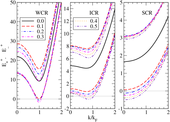
Figure 1.26: Dispersion relations for quasiparticle spectra in the case of the BCS condensate, as functions of momentum in units of Fermi momentum. For each asymmetry, the upper branch corresponds to $E^{+}_{+}$, and the lower to the $E^{+}_{-}$ solution.

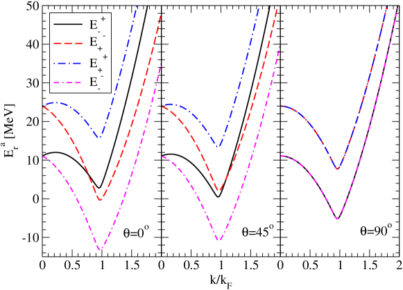
Figure 1.27: Dispersion relations for quasiparticle spectra in the LOFF phase in the WCR, as functions of momentum for three angles and $\alpha=0.49$.

The dispersion relations for quasiparticles in the LOFF phase for special angles $\theta$ are shown in Fig. 1.27 in the WCR and for $\alpha=0.49$ corresponding to the LOFF phase as ground state. In this case, we show all four branches of quasiparticle spectrum. Consistent with the earlier discussion of Figs. 1.11 and 1.25 for $\theta=90\degree$, the LOFF phase resembles the BCS phase and there is a large mismatch between the spectra of protons and neutrons. In this case the branches $a=+$ and $a=-$ are degenerated. For other angles we see again that the nonzero CM momentum mitigates the asymmetry and brings the quasiparticle spectra closer together, i.e., the LOFF phase resembles the symmetrical BCS phase for the two branches with $a\neq r$ for $\theta<90\degree$. This is particularly clear for $\theta=45\degree$, in which case two of the four dispersion relations coincide in the vicinity of the Fermi momentum. It is clear that the optimal mitigation of the isospin mismatch by the finite moment does not need to be for $\theta=0\degree$, but can occur at some angle $0\degree\leq\theta\leq 90\degree$; it is seen that for $\theta=0\degree$ the branches cross and, hence, “overshoot” the optimal compensation.

The restoration of the coherence (Fermi-surface overlap) in the LOFF phase can be illustrated by looking at the solutions of $\epsilon_{n/p,\uparrow/\downarrow}^{\pm}=0$ [see Eq. (1.15)] which define the Fermi-surface in the limit $\Delta\to 0$ but $Q\neq 0$. Solutions for $\epsilon_{n}^{-}=0$ and $\epsilon_{p}^{+}=0$ with ${\bm{Q}}=Q\bm{e}_{z}$ are illustrated in Fig. 1.28 in two cases $Q=0$ and $Q\neq 0$. In both cases we calculated with the effective mass and the chemical potentials we obtained for the LOFF phase in the WCR at $\alpha=0.49$. In the first case the Fermi surfaces are concentric spheres which have no intersection. In the second case the non-zero CM leads to an intersection of the Fermi-spheres; in these regions of intersection the pair-correlations are restored to the magnitude characteristic to the BCS phase. Of course, the CM momentum costs positive kinetic energy, which must be smaller than the negative condensation energy for LOFF phase to be stable.

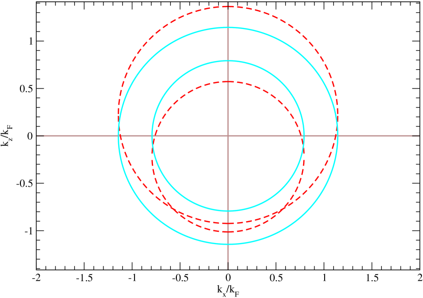
Figure 1.28: Illustration of Fermi surfaces in the LOFF phase. It is characterized by the following values of parameters: $\alpha=0.49$, $\delta\mu=6.45$ MeV, $\Delta=1.27$ MeV and $Q=0.40$ fm^-1. The dashed lines are the actual results for the LOFF phase; by the calculations of the solid lines we use the effective mass and chemical potentials of the LOFF phase in the WCR with $\alpha=0.49$, but we set ${\bm{Q}}=0$.

1.4 Conclusion

Low-density nuclear matter is predicted to feature a rich phase diagram at low temperatures and nonzero isospin asymmetry. The phase diagram contains at least the following phases: the translationally and rotationally symmetric, but isospin-asymmetrical BCS phase, the BEC phase containing neutron-proton dimers, the current carrying Larkin-Ovchinnikov-Fulde-Ferrell phase, and associated phase-separated phases.

Our analysis of these phases can be summarized as follows:

• The phase diagram of nuclear matter composed of these phases has two tri-critical points in general, one of which is a Lifshitz point. These can combine in a tetra-critical point for a special combination of density, temperature, and isospin asymmetry. Tri-critical points exist only for $0<\alpha<\alpha_{\mathrm{LOFF}}$. The phase diagram contains two types of crossovers from the asymmetrical BCS phase to the BEC of deuterons and an embedded neutron gas: a transition between the homogeneous BCS-BEC phases at relatively high temperatures and between the heterogeneous BCS-BEC phases at low temperatures. We have shown that the LOFF phase exists only in a narrow strip in the high-density, low-temperature domain and at nonzero asymmetries.

• The crossovers of BCS-BEC type are smooth and are characterized by lines in the temperature-density plane that do not change much with isospin asymmetry. These lines were obtained by examining the sign of the average chemical potential.

• Detailed analysis of key intrinsic quantities, including the kernel of the gap equation along with the Cooper-pair wave function and its probability density, clearly establishes that in the BCS limit one deals with a coherent state, whose wave function oscillates over many periods with a wavelength characterized by the inverse Fermi momentum $k_{F}^{-1}$. In the opposite limit the wave function is well-localized around the origin, indicating that one is then dealing with a Bose condensate of strongly bound states, namely deuterons. For high densities and high asymmetries, when matter is stable in the LOFF phase, an oscillation emerges belonging to the inverse Cooper-pair momentum $Q^{-1}$, additional to the one belonging to $k_{F}^{-1}$.

• The analysis of the kernel of the wave function, the occupation probabilities of neutrons and protons, and the quasiparticle dispersion relations demonstrates the prominent role played by the Pauli-blocking region (called “the breach”) [67] that appears in these quantities. In the BCS phase and the low-temperature limit of the weak-coupling regime (WCR), the blocking region embraces modes in the range $k_{1}\leq k\leq k_{2}$ around the Fermi surface. In this modal region, it has been found that (a) the minor constituents (protons) are extinct; (b) there are no contributions to the kernel of the gap equation from these modes; and (c) the end of points of this region correspond to the onset of gapless modes that can be excited without any energy cost. The LOFF phase appearing in this regime substantially mitigates the blocking mechanism by allowing for nonzero CM momentum of the condensate. As a consequence, all the intrinsic quantities studied are much closer to those of the isospin-symmetric BCS state.

• We have traced the evolution of the targeted intrinsic properties into the strong-coupling regime (SCR) as the system crosses over from the BCS condensate to a BEC of deuterons plus a neutron gas. In the SCR the long-range coherence of the condensate is lost. The dispersion relations change their form from a spectrum having a minimum at the Fermi surface to a spectrum that is minimal at $k=0$, as would be expected for a BEC, independent of isospin asymmetry. With increasing isospin asymmetry, the proton dispersion relation acquires points with zero excitation energy in this regime. The occupation numbers reach a maximum for finite $k$ and reflect a change of topology at large asymmetries: the filled “Fermi sphere” becomes an empty “core.”

The present investigation of BCS-BEC crossovers with inclusion of unconventional phases, such as the LOFF phase and the heterogeneous phase-separated phase, could be useful in the studies of spin/flavor-imbalanced fermionic systems in ultracold atomic gases, for recent studies see, e.g., [1, 2, 3], dense quark matter, e.g., [4, 5, 6, 7, 8], and other related quantum systems.

Chapter 2 Hartree-Fock

2.1 Introduction

This chapter describes matter in strong magnetic fields which may occur in compact stars [48, 47, 42, 43, 44, 45, 46]. After the hydrogen burning process, a star develops into a red giant or a red supergiant, depending on its mass. After the state of a planetary nebular or a supernova, respectively, the star finely results in a compact star, namely white dwarf, neutron star or black hole. Matter in stellar objects can occur in the form of ordinary baryonic matter either in confined (hadronic) or deconfined (quark-gluon) state. It can also occur in the form of strange matter if the hypothesis that the strange matter is the absolute ground state of matter is true [43]. In this chapter we do not discuss strange matter; its physics is described for example in Refs. [43, 44, 45]. The ordinary baryonic matter in strong magnetic fields has been studied extensively in the literature, see e.g. Ref. [42]. The surface magnetic field of a white dwarf is $B\approx 10^{6}-10^{8}\,$G and the surface magnetic field of a neutron star is $B\approx 10^{12}\,$G [47]. Neutron stars with strong magnetic fields (known as magnetars) with a surface magnetic field of $B\approx 10^{14}-10^{15}\,$G have been observed. It is further conjectured that magnetic fields of the order of $B\approx 10^{18}\,$G can exist in the interiors of magnetars [42, 43, 44, 45, 47]. Due to the virial theorem, the magnetic field can not exceed $B\approx 10^{18}\,$G in the interior of a neutron star and $B\approx 10^{12}\,$G in the interior of a white dwarf [47]. It is estimated that the magnetic field in self-bound compact stars made of strange quark matter cannot exceed $B\approx 10^{20}\,$G [69]. Moreover, strong magnetic fields ($B\approx 10^{16}-10^{17}\,$G) have been considered in newly-born neutron stars [46]. Magnetic fields of order $B\gtrsim 10^{17}\,$G can substantially affect the composition of the outer crust of a neutron star [46]. A discussion of the composition of the outer crust can be found in Ref. [48, 70, 71]. A recent study of the composition of crustal matter in relation to the magnetic field can be found in Ref. [46]. One source of the changes in the composition of the crust in strong magnetic field is the Landau quantization of electron orbits. It has been found that strong magnetic fields favor more isospin-symmetric nuclei in the outer crust of a neutron star. Macroscopically strong magnetic fields act to make the crust of a magnetar more massive than its non-magnetized counterpart [46]. Due to the lower mass of the progenitor stars of white dwarfs, white dwarfs consist of lighter elements than the neutron star crust; massive white dwarfs are conjectured to consist largely of carbon and oxygen [48]. The third element we study in this chapter, neon, can also be found in white dwarfs. These relatively light elements can also occur in accreting neutron stars.

In this introduction 2.1 we give an overview of the Hartree-Fock theory, which is used to compute the properties of nuclei in strong magnetic fields. The discussion follows mostly Refs. [49] and [50]. In Section 2.2 we give an overview of the code Sky3D [50] which was used in numerical computations. In Section 2.3 we describe the extension of the Hartree-Fock theory to include magnetic fields. The corresponding modifications to the code are described. Further we present our results and discussion.

Nuclear systems can be described at different levels of sophistication and precision. At the most fundamental level to describe strongly interacting matter one needs to start from the quantum chromodynamics (QCD). However, it is more rational to start from the nucleon-nucleon interaction to describe bound states of nucleons which form the nuclei. The methods which rely on the basic nucleon-nucleon interaction fitted to the empirical data as a starting point are called ab initio methods. Ab initio calculations are numerically very expensive. The ultimate goal of an ab initio theory is to start from basic microscopic interactions and to predict the properties of a complex compound. This program, however, is not yet realized, although there are no fundamental obstacles. Indeed, for molecules and solids where the basic Coulomb interaction is well known such a program works well. To circumvent the difficulties in the case of finite nuclei or nuclear matter, approximations like restricting to the low-momentum regime or chiral perturbation theory have been applied with increasing success. Within these approximations, many-body methods are exploited to obtain the fully correlated nuclear state, although often one restricts to the mean-field state (Slater determinant or BCS state).

On the other extreme is the macroscopic nuclear liquid-drop model (LDM). It parameterizes the energy of a nucleus in terms of its bulk properties. The parameters of the model are obtained from extensive fits to a large pool of ground-state data of nuclei. The necessary quantum effects, which are not explicit in the LDM, can be added for an improvement of the model. In-between these methods there is the so-called microscopic-macroscopic (mic-mac) method, which combines the single particle model and LDM approaches. The mic-mac method relies on a large amount of preconceived knowledge, in particular on the expected nuclear mean field. It has disadvantages caused by uncertainties when it is extrapolated to the unknown regime of exotic nuclei and it is restricted to ground-state properties.

Another class of “intermediate” approaches is based on the self-consistent mean-field (SCMF). They work at the microscopic level, but they employ effective interactions. Like the vast majority of microscopic models that describe many-body systems, they use a description in terms of single-particle (s.p.) wave functions. SCMF models generate the optimal one-body potential corresponding to the s.p. wave functions starting from various types of zero-range or finite-range effective interactions. Widely used interactions are the Skyrme (zero-range) interaction and the Gogny (finite range) interaction. The effective interaction, as opposed to the bare nucleon-nucleon interaction is “soft” and therefore the Hartree-Fock (HF) theory can be straighforwardly applied. One thus obtains the s.p. wave functions variationally for a given effective interaction, which is calibrated to reproduce the empirical data. The great strength of SCMF is that they reach a high-quality description of ground-state properties, excitations and large-amplitude dynamics. (Covariant versions of SCMF methods based on meson picture of interaction between nuclei and relativistic mean-field (RMF) approach have also been used with success to describe nuclei.)

Correlations in nuclei can be divided roughly into short-range, long-range and collective correlations. The short-range correlations describe the hard repulsive core within the range $r\leq 0.5\,$fm. The long-range correlations act over long distances, which are characterized by coherence lengths that are larger than the interparticle distance. Collective correlations refer to e.g. the center-of-mass motion or rotation of a nucleus. The short- and long-range correlations are fully active in the nuclear volume, their effects can be expressed via smoothly varying functions of densities and currents. This can be summarized in an effective energy-density functional or in an effective interaction. Short- and long-range correlations have been a priori built into the mean-field model. They should not be computed again with effective interactions. Collective correlations on the other hand cannot be transferred to a simple effective functional and need a posteriori treatment.

2.2 Overview of the TDHF Code

2.2.1 Introduction

The calculations reported in this chapter were done with the TDHF code Sky3D [50]. Below we mostly follow Ref. [50] but we discuss in some detail the effects of the magnetic field. These were included in the code in manner similar to the inclusion of the angular momentum in cranking term described in Ref. [72]. In addition we have included the effects of the interaction between the magnetic field and the spin of the nucleons.

The code Sky3D contains a useful selection of Skyrme forces. However it does not contain all terms that have been included in some recent works which aim a high precision description of nuclear systems. Therefore the Skyrme interaction used in Sky3D is useful for a semiquantitative description, where high precision of the Skyrme force is not decisive. (These additional terms can be added to the code without much difficulty).

The code Sky3D solves the static or dynamic equations of motion using Skyrme-like forces on a three-dimensional Cartesian grid. Certain symmetries are assumed when imposing isolated or periodic boundary conditions. Consequently the nucleonic wave function spinors are always periodic functions, while it is possible to choose an isolated charge distribution for the Coulomb potential. Due to the possibility of choosing periodic boundary conditions and due to the highly flexible initialization, the code is also suitable for astrophysical nuclear matter applications. All spatial derivatives in the code are calculated with the finite Fourier transform method. For the static Hartree-Fock equations a damped gradient iteration method is used and for the time-dependent Hartree-Fock (TDHF) equations an expansion of the time-development operator is employed. It is possible to place any number of initial nuclei into the mesh at arbitrary positions with any velocities. It is also possible to include pairing in the BCS approximation for the static case. However, due to the absence of some time-odd terms in the implementation of the Skyrme interaction, calculations may be restricted only to even-even nuclei. Altogether the code Sky3D can be used (within the limitations of mean-field theory) for a wide variety of applications in nuclear structure, collective excitations, and nuclear reactions.

An overview of the code Sky3D is included in Ref. [50] to offer the possibility to include additional physics or special analysis of the results. In this chapter and in appendix B we give an overview of the code and add the extensions which are needed for the inclusion of magnetic fields.

2.2.2 Physics implemented in the code

Here we give a brief discussion of the physics implemented in the code which is important for the studies of this chapter. See appendix B and Ref. [50] for further details.

In the mean-field theory, the many-body system is described in terms of a set of single-particle (s.p.) wave functions. With these s.p. wave functions local densities and currents can be defined, see appendix B.1.

The code Sky3D solves the mean-field equations based on the widely used Skyrme energy functional. The energy-density functional contains an expansion in a number of derivatives, i.e., it corresponds to a low-momentum expansion of many-body theory (see Ref. [49]). The energy functional as implemented in the code can be written as

$$E_{\mathrm{tot}} = T+(E_{0}+E_{1}+E_{2}+E_{3}+E_{\mathrm{ls}})$$ (2.1)

$$+E_{\mathrm{Coulomb}}+E_{\mathrm{pair}}+E_{\mathrm{corr}}\,,$$

where the terms which arise from the Skyrme force are collected within the parenthesis. The various terms of Eq. (2.1) are defined in appendix B.2.

The variation of the energy-density functional discussed above with $\partial_{\psi_{\alpha}^{*}}E=\hat{h}\psi_{\alpha}$ leads to the mean-field Hamiltonian $\hat{h}$. It is given by

$$\hat{h}_{q} = U_{q}(\bm{r})-\nabla\cdot\left[B_{q}(\bm{r})\nabla\right]+\mathrm{i}\bm{W}_{q}\cdot\left({\bm{\sigma}}\times\nabla\right)+{\bm{S}}_{q}\cdot{\bm{\sigma}}$$ (2.2)

$$-\tfrac{\mathrm{i}}{2}\left[\left(\nabla\cdot\bm{A}_{q}\right)+2\bm{A}_{q}\cdot\nabla\right]\,,$$

with $q\in\{p,n\}$ specifying the isospin. The terms are discussed in appendix B.4, using the force coefficients of appendix B.3. Note that because protons are charged, the Coulomb potential acting between protons should be added to the potential.

With the Hamiltonian operator the eigenvalues of the system can be computed through the Schrödinger equation

$$\hat{h}\psi_{\alpha}=\varepsilon_{\alpha}\psi_{\alpha}\,,$$ (2.3)

with $\hat{h}$ being the mean-field Hamiltonian of Eq. (2.2) and $\varepsilon_{\alpha}$ being the single-particle energy of state $\alpha$. This equation follows upon variation with respect to single-particle wave-function $\psi_{\alpha}$. In the code Sky3D, pairing can be included in the BCS approximation. See appendix B.5 for more details on the static calculations without pairing. For more details also on static Hartree-Fock including pairing and on time-dependent Hartree-Fock see [50].

As an output, the code provides several observables, e.g. the total deformation $\beta$, the triaxiality $\gamma$ and the r.m.s radii $r_{\mathrm{rms}}^{q}$. See appendix B.6 for further details on the observables.

The calculations of Sky3D run on a three dimensional regular Cartesian grid. The number of grid points and the distance between the grid points can be chosen by the user. The code uses a fast Fourier transform and therefore periodic boundary conditions, except for the Coulomb force.

A particular strength of the code Sky3D is the possibility of a flexible initialization. For the calculations of this chapter, we used the harmonic oscillator initialization. Here the user can implement the radii of the harmonic oscillator states in each spatial direction. Moreover, it is possible to choose the numbers of neutrons and protons and it is also possible to include unoccupied neutron and proton states. When using unoccupied states, there are more nucleon states calculated than the actual existing ones. This can lead to a faster convergence. Initially the harmonic oscillator states are filled up. For certain set-ups, e.g., if we consider magnetic fields, some normally higher harmonic oscillator states may be energetically favored, but not taken into account by using only occupied states. In this case it can happen that the code converges to two different configurations, whether we use unoccupied states or not; or it can happen that the code is stuck in one configuration for a long time, before it converges to the lower energy state without the additional unoccupied states.

2.3 Hartree-Fock with magnetic field

2.3.1 Introduction

Now we turn to the central problem of this chapter – the determination of the properties of nuclei in strong magnetic fields. To introduce the magnetic field the Hamiltonian (2.2) is modified as

$$\hat{h}_{\mathrm{mod},\,q} = \hat{h}_{q}+\hat{h}_{\mathrm{mag},\,q}\,,$$ (2.4a)

$$\hat{h}_{\mathrm{mag},\,q} = -\left({\bm{l}}\cdot\delta_{q,p}+g_{q}\frac{{\bm{\sigma}}}{2}\right)\cdot\tilde{\bm{B}}_{q}\,,$$ (2.4b)

with $q\in\{p,n\}$ specifying the isospin, ${\bm{\sigma}}$ is the spin Pauli matrix and ${\bm{l}}$ is the (dimensionless) orbital angular momentum related to the spin ${\bm{S}}$ and the orbital angular momentum ${\bm{L}}$ via ${\bm{S}}=\hbar{\bm{\sigma}}/2$ and ${\bm{L}}=\hbar{\bm{l}}$, where $g_{n}=-3.82608544$ and $g_{p}=5.584694712$ are the Landé $g$-factors of neutrons and protons and

$$\tilde{{\bm{B}}_{q}}=\frac{e\hbar}{2\,m_{q}c}{\bm{B}}\,,$$ (2.5)

where ${\bm{B}}$ being the magnetic field. The Kronecker Delta is due to the fact that neutrons are charge neutral and thus do not couple to the orbital angular momentum. Despite their charge neutrality, they couple to the spin because of the charge distribution of the constituent quarks. If dipole modes are considered, effective currents for neutrons and protons should be introduced; neutrons get a negative effective charge and the proton charge is reduced [73]. Due to the interactions of the nucleons within the nucleus, the $g$ factors are modified, and one should include quenching factors as it is done in [49]. These quenching factors are known for random-phase approximation (RPA), but not for our studies, therefore we can not adopt them. However, without these quenching factors, the results are only qualitative.

Using a constant magnetic field in $\bm{e}_{z}$ direction (${\bm{B}}=B_{z}\bm{e}_{z}$) allows us to simplify the equations to the form

$$\hat{h}_{\mathrm{mod},\,q} = \hat{h}_{q}-\left(l_{z}\cdot\delta_{q,p}+g_{q}\frac{\sigma_{z}}{2}\right)\cdot\tilde{B}_{q,z}\,,$$ (2.6a)

$$\hat{h}_{\mathrm{mod},\,q} = \hat{h}_{q}+\left(\mathrm{i}(x\partial_{y}-y\partial_{x})\delta_{q,p}+\frac{g_{q}}{2}\begin{pmatrix}-1&0\\ 0&1\end{pmatrix}\right)\cdot\tilde{B}_{q,z}\,.$$ (2.6b)

The additional terms due to the magnetic field appearing in Eq. (2.4) are implemented in the module Meanfield of the code.

2.3.2 Clebsch-Gordan coefficients

The definition of the Clebsch-Gordan coefficients follows the book of Greiner and Maruhn [73]. We need the general formula

$$\left|JMls\right> = \sum_{m_{l}m_{s}}\left|lm_{l}sm_{s}\right>(lsJ|m_{l}m_{s}M)\,,$$ (2.7)

hereby $l$ is the orbital angular momentum, $s$ the spin and $J$ the total angular momentum and $m_{l}$, $m_{s}$ and $M$ are the $z$-components of $l$, $s$ or $J$, respectively. The following conditions need to be fulfilled:

$$m_{l}+m_{s} = M\,,$$ (2.8a)

$$|l-s| \leq J\leq l+s\,.$$ (2.8b)

In our case we deal with nucleons, which have $s=1/2$ and thus have $m_{s}=\pm 1/2$. For $l$ we have non-negative integer numbers, for $m_{l}$ we obtain integer numbers, which can be positive or negative or zero. Thus we have non-negative half-integer numbers for $J$ and we obtain half-integer numbers, which can be positive or negative for $M$. For clarity we introduce the following conventions:

• $s$ is always $1/2$, therefore it is skipped.

• $m_{s}$ is always $\pm 1/2$. To prevent confusion with other terms, it is written in the following way:

  • $m_{s}=\uparrow$ for $m_{s}=+1/2$

  • $m_{s}=\downarrow$ for $m_{s}=-1/2$

• $l$ is always positive, it is always written without sign.

• $m_{l}$ is always written with sign to prevent confusion with $l$.

• For $J$ and $M$ the same conventions as for $l$ and $m_{l}$ are introduced. There is no confusion between $J$, $M$ and $l$, $m_{l}$, because the former are half-integer and the latter are integer numbers.

Thus, to summarize our convention,

$s$		skipped
$m_{s}$		$\uparrow$ or $\downarrow$
$l$	without sign	integer number
$m_{l}$	with sign	integer number
$J$	without sign	half-integer number
$M$	with sign	half-integer number

Now we can introduce the Clebsch-Gordan coefficients for $s_{1/2}$, $p_{3/2}$ and $p_{1/2}$ states

$$\left|J,M,l\right> = \sum_{m_{l},m_{s}}\left|l,m_{l},m_{s}\right>$$ (2.9a)

$$\times\left(l,J\middle|m_{l},m_{s},M\right)\,,$$

$$s_{1/2},M=-\tfrac{1}{2}:\quad\left|\tfrac{1}{2},-\tfrac{1}{2},0\right> = \left|0,+0,\downarrow\right>\left(0,\tfrac{1}{2}\middle|+0,\downarrow,-\tfrac{1}{2}\right)\,,$$ (2.9b)

$$s_{1/2},M=+\tfrac{1}{2}:\quad\left|\tfrac{1}{2},+\tfrac{1}{2},0\right> = \left|0,+0,\uparrow\right>\left(0,\tfrac{1}{2}\middle|+0,\uparrow,+\tfrac{1}{2}\right)\,,$$ (2.9c)

$$p_{3/2},M=-\tfrac{3}{2}:\quad\left|\tfrac{3}{2},-\tfrac{3}{2},1\right> = \left|1,-1,\downarrow\right>\left(1,\tfrac{3}{2}\middle|-1,\downarrow,-\tfrac{3}{2}\right)\,,$$ (2.9d)

$$p_{3/2},M=-\tfrac{1}{2}:\quad\left|\tfrac{3}{2},-\tfrac{1}{2},1\right> = \left|1,-1,\uparrow\right>\left(1,\tfrac{3}{2}\middle|-1,\uparrow,-\tfrac{1}{2}\right)$$ (2.9e)

$$+\left|1,+0,\downarrow\right>\left(1,\tfrac{3}{2}\middle|+0,\downarrow,-\tfrac{1}{2}\right)\,,$$

$$p_{3/2},M=+\tfrac{1}{2}:\quad\left|\tfrac{3}{2},+\tfrac{1}{2},1\right> = \left|1,+0,\uparrow\right>\left(1,\tfrac{3}{2}\middle|+0,\uparrow,+\tfrac{1}{2}\right)$$ (2.9f)

$$+\left|1,+1,\downarrow\right>\left(1,\tfrac{3}{2}\middle|+1,\downarrow,+\tfrac{1}{2}\right)\,,$$

$$p_{3/2},M=+\tfrac{3}{2}:\quad\left|\tfrac{3}{2},+\tfrac{3}{2},1\right> = \left|1,+1,\uparrow\right>\left(1,\tfrac{3}{2}\middle|+1,\uparrow,+\tfrac{3}{2}\right)\,,$$ (2.9g)

$$p_{1/2},M=-\tfrac{1}{2}:\quad\left|\tfrac{1}{2},-\tfrac{1}{2},1\right> = \left|1,-1,\uparrow\right>\left(1,\tfrac{1}{2}\middle|-1,\uparrow,-\tfrac{1}{2}\right)$$ (2.9h)

$$+\left|1,+0,\downarrow\right>\left(1,\tfrac{1}{2}\middle|+0,\downarrow,-\tfrac{1}{2}\right)\,,$$

$$p_{1/2},M=+\tfrac{1}{2}:\quad\left|\tfrac{1}{2},+\tfrac{1}{2},1\right> = \left|1,+0,\uparrow\right>\left(1,\tfrac{1}{2}\middle|+0,\uparrow,+\tfrac{1}{2}\right)$$ (2.9i)

$$+\left|1,+1,\downarrow\right>\left(1,\tfrac{1}{2}\middle|+1,\downarrow,+\tfrac{1}{2}\right)\,,$$

which by inserting the Clebsch-Gordan coefficients reduce to

$$s_{1/2},M=-\tfrac{1}{2}:\quad\left|\tfrac{1}{2},-\tfrac{1}{2},0\right> = \left|0,+0,\downarrow\right>\,,$$ (2.10a)

$$s_{1/2},M=+\tfrac{1}{2}:\quad\left|\tfrac{1}{2},+\tfrac{1}{2},0\right> = \left|0,+0,\uparrow\right>\,,$$ (2.10b)

$$p_{3/2},M=-\tfrac{3}{2}:\quad\left|\tfrac{3}{2},-\tfrac{3}{2},1\right> = \left|1,-1,\downarrow\right>\,,$$ (2.10c)

$$p_{3/2},M=-\tfrac{1}{2}:\quad\left|\tfrac{3}{2},-\tfrac{1}{2},1\right> = \tfrac{1}{\sqrt{3}}\left|1,-1,\uparrow\right>$$ (2.10d)

$$+\sqrt{\tfrac{2}{3}}\left|1,+0,\downarrow\right>\,,$$

$$p_{3/2},M=+\tfrac{1}{2}:\quad\left|\tfrac{3}{2},+\tfrac{1}{2},1\right> = \sqrt{\tfrac{2}{3}}\left|1,+0,\uparrow\right>$$ (2.10e)

$$+\tfrac{1}{\sqrt{3}}\left|1,+1,\downarrow\right>\,,$$

$$p_{3/2},M=+\tfrac{3}{2}:\quad\left|\tfrac{3}{2},+\tfrac{3}{2},1\right> = \left|1,+1,\uparrow\right>\,,$$ (2.10f)

$$p_{1/2},M=-\tfrac{1}{2}:\quad\left|\tfrac{1}{2},-\tfrac{1}{2},1\right> = -\sqrt{\tfrac{2}{3}}\left|1,-1,\uparrow\right>$$ (2.10g)

$$+\tfrac{1}{\sqrt{3}}\left|1,+0,\downarrow\right>\,,$$

$$p_{1/2},M=+\tfrac{1}{2}:\quad\left|\tfrac{1}{2},+\tfrac{1}{2},1\right> = -\tfrac{1}{\sqrt{3}}\left|1,+0,\uparrow\right>$$ (2.10h)

$$+\sqrt{\tfrac{2}{3}}\left|1,+1,\downarrow\right>\,.$$

We can now calculate the $z$-components of the orbital angular momentum and the spin with the following definition

$$\left<\mathcal{O}(J,M,l)\right>=\left<J,M,l\middle|\mathcal{O}(J,M,l)\middle|J,M,l\right>\,,$$ (2.11)

and using the following relations

$$\left<l,m_{l}\middle|\frac{L_{z}}{\hbar}\middle|l,m_{l}^{\prime}\right>= m_{l}\delta_{m_{l},m_{l}^{\prime}}\,, \quad\left<l,m_{l}\middle|l,m_{l}^{\prime}\right>= \delta_{m_{l},m_{l}^{\prime}}\,,$$ (2.12a)

$$\left<m_{s}\middle|\frac{S_{z}}{\hbar}\middle|m_{s}^{\prime}\right>= m_{s}\delta_{m_{s},m_{s}^{\prime}}\,, \quad\left<m_{s}\middle|m_{s}^{\prime}\right>= \delta_{m_{s},m_{s}^{\prime}}\,.$$ (2.12b)

For the orbital angular momentum we obtain

$$\left<\frac{L_{z}(J,M,l)}{\hbar}\right> = \left<J,M,l\middle|\frac{L_{z}}{\hbar}\middle|J,M,l\right>$$

$$= \sum_{m_{l},m_{l}^{\prime},m_{s},m_{s}^{\prime}}\left<l,m_{l},m_{s}\middle|\frac{L_{z}}{\hbar}\middle|l,m_{l}^{\prime},m_{s}^{\prime}\right>$$

$$\times\left(l,J|m_{l},m_{s},M\right)\left(l,J|m_{l}^{\prime},m_{s}^{\prime},M\right)$$

$$= \sum_{m_{l},m_{s}}\left<l,m_{l},m_{s}\middle|\frac{L_{z}}{\hbar}\middle|l,m_{l},m_{s}\right>\left(l,J|m_{l},m_{s},M\right)^{2}$$

$$= \sum_{m_{l},m_{s}}\left(l,J|m_{l},m_{s},M\right)^{2}\left<l,m_{l}\middle|\frac{L_{z}}{\hbar}\middle|l,m_{l}\right>\left<m_{s}\middle|m_{s}\right>$$

$$\Rightarrow\left<\frac{L_{z}(J,M,l)}{\hbar}\right> = \sum_{m_{l},m_{s}}m_{l}\cdot\left(l,J|m_{l},m_{s},M\right)^{2}\,.$$ (2.13b)

In an analogous manner we evaluate the spin component

$$\left<\frac{S_{z}(J,M,l)}{\hbar}\right> = \left<J,M,l\middle|\frac{S_{z}}{\hbar}\middle|J,M,l\right>$$ (2.14a)

$$\Rightarrow\left<\frac{S_{z}(J,M,l)}{\hbar}\right> = \sum_{m_{l},m_{s}}m_{s}\cdot\left(l,J|m_{l},m_{s},M\right)^{2}\,.$$ (2.14b)

Performing the summation and calculating the Clebsch-Gordan coefficients gives

$$s_{1/2},M= -\tfrac{1}{2}: \quad\left<L_{z}\right>= +0\cdot\hbar\,, \quad\left<S_{z}\right>= -\tfrac{1}{2}\cdot\hbar\,,$$ (2.15a)

$$s_{1/2},M= +\tfrac{1}{2}: \quad\left<L_{z}\right>= +0\cdot\hbar\,, \quad\left<S_{z}\right>= +\tfrac{1}{2}\cdot\hbar\,,$$ (2.15b)

$$p_{3/2},M= -\tfrac{3}{2}: \quad\left<L_{z}\right>= -1\cdot\hbar\,, \quad\left<S_{z}\right>= -\tfrac{1}{2}\cdot\hbar\,,$$ (2.15c)

$$p_{3/2},M= -\tfrac{1}{2}: \quad\left<L_{z}\right>= -\tfrac{1}{3}\cdot\hbar\,, \quad\left<S_{z}\right>= -\tfrac{1}{6}\cdot\hbar\,,$$ (2.15d)

$$p_{3/2},M= +\tfrac{1}{2}: \quad\left<L_{z}\right>= +\tfrac{1}{3}\cdot\hbar\,, \quad\left<S_{z}\right>= +\tfrac{1}{6}\cdot\hbar\,,$$ (2.15e)

$$p_{3/2},M= +\tfrac{3}{2}: \quad\left<L_{z}\right>= +1\cdot\hbar\,, \quad\left<S_{z}\right>= +\tfrac{1}{2}\cdot\hbar\,,$$ (2.15f)

$$p_{1/2},M= -\tfrac{1}{2}: \quad\left<L_{z}\right>= -\tfrac{2}{3}\cdot\hbar\,, \quad\left<S_{z}\right>= +\tfrac{1}{6}\cdot\hbar\,,$$ (2.15g)

$$p_{1/2},M= +\tfrac{1}{2}: \quad\left<L_{z}\right>= +\tfrac{2}{3}\cdot\hbar\,, \quad\left<S_{z}\right>= -\tfrac{1}{6}\cdot\hbar\,.$$ (2.15h)

Let us now have a closer look at these coefficients. In all states we obtain $M=m_{l}+m_{s}=(\left<L_{z}\right>+\left<S_{z}\right>)/\hbar$ as a good quantum number. However we only obtain $\left<L_{z}\right>=\hbar\,m_{l}$ and $\left<S_{z}\right>=\hbar\,m_{s}$ as a good quantum number for states with pure Clebsch-Gordan coefficients. Hereby “pure” refers to Clebsch-Gordan coefficients where one $\left|J,M,L\right>$ state refers to one $\left|l,m_{l},m_{s}\right>$ state and “mixed” refers to those, where $\left|J,M,L\right>$ are formed by superpositions of $\left|l,m_{l},m_{s}\right>$ states. For the states with mixed Clebsch-Gordan coefficients, this differs due to the l-s coupling. In these states, $\left<L_{z}\right>$ and $\left<S_{z}\right>$ are superpositions of one state with $|{m_{l}}|=l$ and one with $|{m_{l}}|<l$. The quantum numbers $m_{l}$ and $m_{s}$ and the resulting $M=m_{l}+m_{s}$ are shown in Fig. 2.1 for different states. We have one solid line at $M=0$ and dashed lines with intervals of $1/2$. The arrows corresponding to $m_{l}$ start at the origin and the ones corresponding to $m_{s}$ start at the end points of the arrows corresponding to $m_{l}$ to present $M$.

We can now also calculate the energy difference of these states according to Eq. (2.4) with the relations of (2.12):

$$\Delta E_{q}(J,M,l) = \left<J,M,l\middle|\hat{h}_{\mathrm{mag},\,q}\middle|J,M,l\right>\,,$$ (2.16a)

$$\Delta E_{q}(J,M,l) = \left<J,M,l\middle|-\tilde{B}_{q}\middle(\frac{L_{z}}{\hbar}\cdot\delta_{q,p}\right.$$ (2.16b)

$$\left.+g_{q}\cdot\frac{S_{z}}{\hbar}\middle)\middle|J,M,l\right>\,.$$

This can be written as

$$\Delta E_{q}(J,M,l) = \left<J,M,l\middle|-\tilde{B}_{q}\middle(\frac{L_{z}}{\hbar}\cdot\delta_{q,p}+g_{q}\cdot\frac{S_{z}}{\hbar}\middle)\middle|J,M,l\right>$$

$$= -\sum_{m_{l},m_{l}^{\prime},m_{s},m_{s}^{\prime}}\left<l,m_{l},m_{s}\middle|\tilde{B}_{q}\middle(\frac{L_{z}}{\hbar}\cdot\delta_{q,p}\right.$$

$$+\left.g_{q}\cdot\frac{S_{z}}{\hbar}\middle)\middle|l,m_{l}^{\prime},m_{s}^{\prime}\right>$$

$$\times\left(l,J|m_{l},m_{s},M\right)\left(l,J|m_{l}^{\prime},m_{s}^{\prime},M\right)$$

$$= -\sum_{m_{l},m_{s}}\left<l,m_{l},m_{s}\middle|\tilde{B}_{q}\middle(\frac{L_{z}}{\hbar}\cdot\delta_{q,p}\right.$$

$$+\left.g_{q}\cdot\frac{S_{z}}{\hbar}\middle)\middle|l,m_{l},m_{s}\right>\left(l,J|m_{l},m_{s},M\right)^{2}$$

$$= -\sum_{m_{l},m_{s}}\left(l,J|m_{l},m_{s},M\right)^{2}$$

$$\times\left(\left<l,m_{l}\middle|\middle<m_{s}\middle|\tilde{B}_{q}\cdot\frac{L_{z}}{\hbar}\cdot\delta_{q,p}\middle|l,m_{l}\middle>\middle|m_{s}\right>\right.$$

$$+\left.\left<l,m_{l}\middle|\middle<m_{s}\middle|\tilde{B}_{q}\cdot g_{q}\cdot\frac{S_{z}}{\hbar}\middle|l,m_{l}\middle>\middle|m_{s}\right>\right)$$

$$= -\sum_{m_{l},m_{s}}\left(l,J|m_{l},m_{s},M\right)^{2}\left(\left<l,m_{l}\middle|\tilde{B}_{q}\cdot\frac{L_{z}}{\hbar}\cdot\delta_{q,p}\middle|l,m_{l}\right>\right.$$

$$\times\left<m_{s}\middle|m_{s}\right>+\left.\left<m_{s}\middle|\tilde{B}_{q}\cdot g_{q}\cdot\frac{S_{z}}{\hbar}\middle|m_{s}\right>\left<l,m_{l}\middle|l,m_{l}\right>\right)$$

$$= -\sum_{m_{l},m_{s}}\left(l,J|m_{l},m_{s},M\right)^{2}\tilde{B}_{q}\left(\delta_{q,p}\left<l,m_{l}\middle|\frac{L_{z}}{\hbar}\middle|l,m_{l}\right>\right.$$

$$\left.+g_{q}\left<m_{s}\middle|\frac{S_{z}}{\hbar}\middle|m_{s}\right>\right)$$

$$\Rightarrow\Delta E_{q}(J,M,l) = -\sum_{m_{l},m_{s}}\left(l,J|m_{l},m_{s},M\right)^{2}\tilde{B}_{q}$$ (2.17b)

$$\times\left(m_{l}\cdot\delta_{q,p}+g_{q}\cdot m_{s}\right)\,.$$

Using Eq. (2.17b) and Eq. (2.10) leads to:

$$s_{1/2},M= -\tfrac{1}{2}: \Delta E_{n}= \tfrac{1}{2}\tilde{B}_{n}\cdot{g_{n}}\,, \Delta E_{p}= \tilde{B}_{p}\cdot\tfrac{g_{p}}{2}\,,$$ (2.18a)

$$s_{1/2},M= +\tfrac{1}{2}: \Delta E_{n}= -\tfrac{1}{2}\tilde{B}_{n}\cdot{g_{n}}\,, \Delta E_{p}= -\tilde{B}_{p}\cdot\tfrac{g_{p}}{2}\,,$$ (2.18b)

$$p_{3/2},M= -\tfrac{3}{2}: \Delta E_{n}= \tfrac{1}{2}\tilde{B}_{n}\cdot{g_{n}}\,, \Delta E_{p}= \tilde{B}_{p}\left(1+\tfrac{g_{p}}{2}\right)\,,$$ (2.18c)

$$p_{3/2},M= -\tfrac{1}{2}: \Delta E_{n}= \tfrac{1}{6}{\tilde{B}_{n}}\cdot{g_{n}}\,, \Delta E_{p}= \tfrac{\tilde{B}_{p}}{3}\left(1+\tfrac{g_{p}}{2}\right)\,,$$ (2.18d)

$$p_{3/2},M= +\tfrac{1}{2}: \Delta E_{n}= -\tfrac{1}{6}{\tilde{B}_{n}}\cdot{g_{n}}\,, \Delta E_{p}= -\tfrac{\tilde{B}_{p}}{3}\left(1+\tfrac{g_{p}}{2}\right)$$ (2.18e)

$$p_{3/2},M= +\tfrac{3}{2}: \Delta E_{n}= -\tfrac{1}{2}\tilde{B}_{n}\cdot{g_{n}}\,, \Delta E_{p}= -\tilde{B}_{p}\left(1+\tfrac{g_{p}}{2}\right)\,,$$ (2.18f)

$$p_{1/2},M= -\tfrac{1}{2}: \Delta E_{n}= -\tfrac{1}{6}{\tilde{B}_{n}}\cdot{g_{n}}\,, \Delta E_{p}= \tfrac{2}{3}\tilde{B}_{p}\left(1-\tfrac{g_{p}}{4}\right)\,,$$ (2.18g)

$$p_{1/2},M= +\tfrac{1}{2}: \Delta E_{n}= \tfrac{1}{6}{\tilde{B}_{n}}\cdot{g_{n}}\,, \Delta E_{p}= -\tfrac{2}{3}\tilde{B}_{p}\left(1-\tfrac{g_{p}}{4}\right)\,.$$ (2.18h)

2.3.3 Results

All calculations used for the following analysis were done on a grid with 32 grid points in each direction and a distance between the grid points of 1.0 fm. For the convergence parameters $\delta$ and $E_{0}$ of Eq. (B.5) we chose $\delta=0.4$ and $E_{0}=100$ as recommended in [50]. For testing, we varied the number of grid points, the distance between the grid points and the convergence parameters, leading to different computational times and different levels of convergence, but not to different physical results. Moreover, we used a fragment initialization with one fragment for testing. For the radii of the harmonic oscillator states we chose 3.0 fm, 3.2 fm and 3.1 fm for the $x$-, $y$- and $z$-direction, respectively. We chose the Skyrme force SV-bas [74] without pairing. The boundary condition for the Coulomb force was implemented with isolated boundary conditions. To achieve a better convergence, we used unoccupied states. We studied nuclei with equal amount of neutrons and protons: [12]C, [16]O and [20]Ne and chose the same number of neutron and proton unoccupied states each. We chose 8 occupied and 8 unoccupied states for [16]O, 10 occupied and 10 unoccupied for [20]Ne and 6 occupied and 4 unoccupied for [12]C. See subsection 2.2.2, appendix B and Ref. [50] for further discussion on the terms in this paragraph.

The magnetic field was chosen in $\bm{e}_{z}$ direction. For testing, also other directions were calculated, leading to the same physical results. For stronger magnetic fields, convergence was not always achieved. Within the code, we used natural units for the magnetic field of $\sqrt{\mathrm{MeV}\,\mathrm{fm}^{-3}}=4.00\cdot 10^{16}\,$G. We started at $B=0$, increased it slightly to $B=0.001\sqrt{\mathrm{MeV}\,\mathrm{fm}^{-3}}=4.00\cdot 10^{13}\,$G. Afterwards we used multiples of $0.25\sqrt{\mathrm{MeV}\,\mathrm{fm}^{-3}}=1.00\cdot 10^{16}\,$G to increment the magnetic field. First, we computed 2000 iterations at $B=0$, then 2000 at $B=0.001\sqrt{\mathrm{MeV}\,\mathrm{fm}^{-3}}$ and then 4000 at each multiple of $0.25\sqrt{\mathrm{MeV}\,\mathrm{fm}^{-3}}$, as long as we reached convergence. For [12]C, a calculation starting at $B=0$ did not give good converging results for stronger magnetic fields. However, a calculation starting at $B=6\sqrt{\mathrm{\mathrm{MeV}\,\mathrm{fm}^{-3}}}$ did. With these steps, we got better convergence for stronger magnetic fields. However, for certain strengths of the magnetic field, no convergence was achieved. Since we got a change of the occupation for protons in [16]O, we changed the step size in this region, see below for discussion.

To access the shape and size of the nuclei we examined the parameters $r_{\mathrm{rms}}\equiv r_{\mathrm{rms}}^{(\mathrm{total})}$ of Eq. (B.7h) and $\beta,\,\gamma$ of Eq. (B.7g). Here $\gamma=0\degree$ refers to a prolate deformed nucleus, $\gamma=60\degree$ refers to an oblate deformed nucleus and angles between $\gamma=0\degree$ and $\gamma=60\degree$ refer to a deformation in a state between prolate and oblate. If $\beta=0$ the nucleus is spherical (undeformed) independent of $\gamma$. For non-zero $\beta$ nuclei are deformed [73].

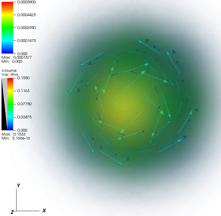
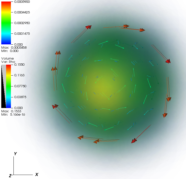
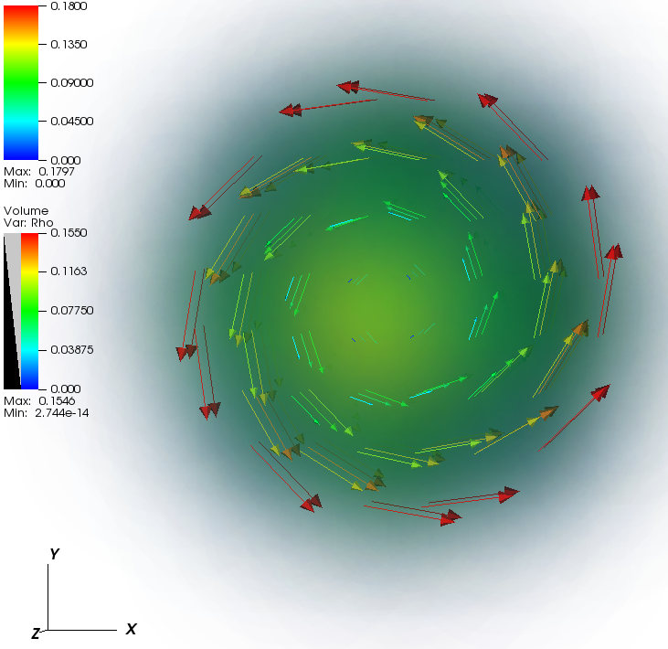
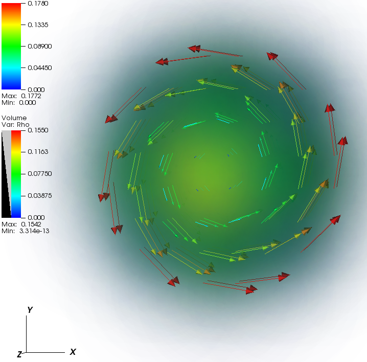
Figure 2.8: The current density divided by the particle density (collective flow velocity) for neutrons (top left) and protons (right and bottom) for [16]O for different values of the magnetic field. Top: $B=3.9\cdot 10^{17}\,$G, bottom left: $B=4.1\cdot 10^{17}\,$G, bottom right: $B=4.7\cdot 10^{17}\,$G. As background the particle density is added. This figure was created with VisIt [51].

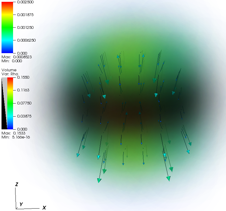
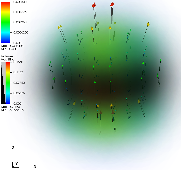
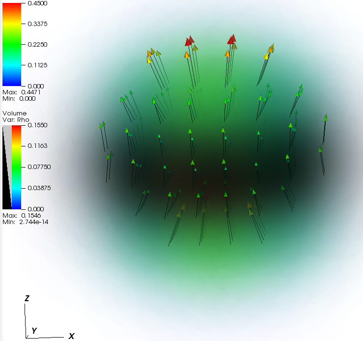
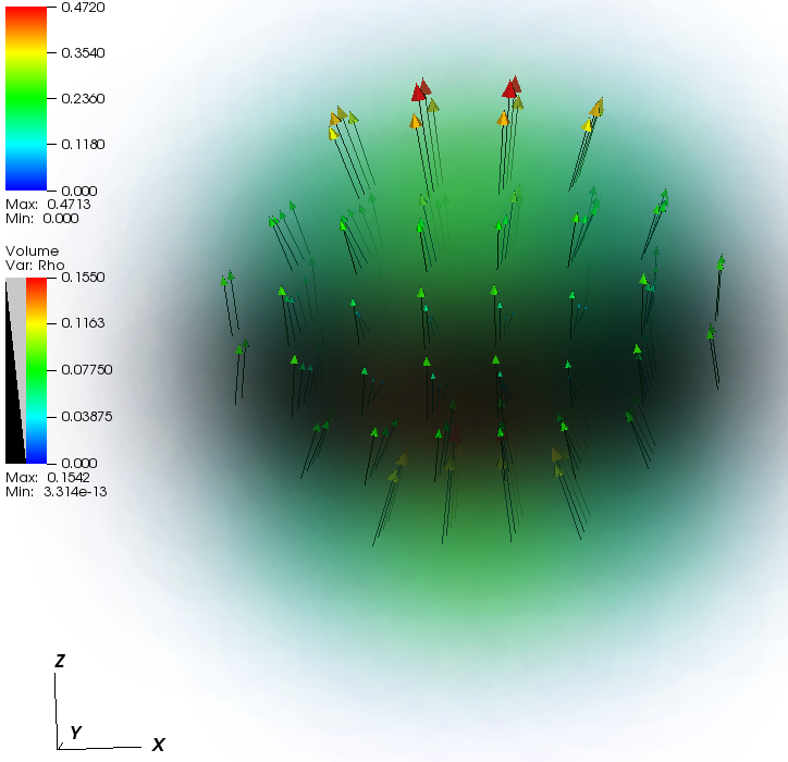
Figure 2.9: The spin density divided by the particle density for [16]O with the same arrangement and magnetic fields as in Fig. 2.8. This figure was created with VisIt [51].

Moreover, we calculated the current and spin densities. We evaluated them separately for neutrons and protons normalised with the particle density. The current density over the particle density results in the collective flow velocity. Since the particle density approaches $0$ outside of the nucleus, we had to do a cut off and displayed these quantities only in the region with $\rho_{n/p}>0.01\,$fm^-3. All figures for the velocity (Figs. 2.8, 2.10 and 2.12) and for the spin (Figs. 2.9, 2.11 and 2.13) are done from the same perspective, respectively. For a specific nucleus, magnetic field and quantity (current or spin density) we used the same scaling for the neutron and proton quantity. To show the position of these vectors relative to the nucleus, we added the particle density ($\rho=\rho_{n}+\rho_{p}$) as background. The scaling of this particle density is always the same for both quantities (current and spin density) for both isospins for all magnetic fields, but differs for different nuclei. These figures were created with VisIt [51]. A note on the corresponding coding of the vectors: In each figure, the magnitudes of the vectors are specified by the length of the vector and by its color. The color changes from red for high values via yellow, green and cyan to blue for low values.

Effects of the magnetic field on [16]O

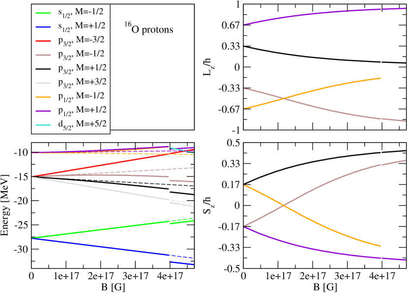
Figure 2.2: The energy levels (analytical (dashed) and numerical (solid)), $\left<L_{z}\right>$ and $\left<S_{z}\right>$ as functions of the magnetic field for protons in [16]O.

We evaluated the effect of the magnetic field on different nuclei. First we want to report our results for [16]O. Here we calculated the energy levels and the $z$-components of orbital angular momentum $\left<L_{z}\right>$ and spin $\left<S_{z}\right>$ of neutrons and protons as functions of the magnetic field. The results are shown in Figs. 2.2 and 2.3. For the states defined in Eqs. (2.10a), (2.10b), (2.10c) and (2.10f) we obtain integer or half-integer numbers for $\left<L_{z}\right>/\hbar$ or $\left<S_{z}\right>/\hbar$ which are identical to the quantum numbers $m_{l}$ or $m_{s}$, respectively, independent of the magnetic field. However, for the states with mixed Clebsch-Gordan coefficients defined in Eqs. (2.10d), (2.10e), (2.10g) and (2.10h), $\left<L_{z}\right>$ and $\left<S_{z}\right>$ change as functions of the magnetic field. In Figs. 2.2 and 2.3 $\left<L_{z}\right>$ and $\left<S_{z}\right>$ are only shown for those state, where $\left<L_{z}\right>$ and $\left<S_{z}\right>$ change as functions of the magnetic field.

We now take a closer look at these states. For all magnetic fields, we obtain $M=m_{l}+m_{s}=(\left<L_{z}\right>+\left<S_{z}\right>)/\hbar$ as a good quantum number. However, for the orbital angular momentum and the spin there are two ranges of values for the magnetic field. In the limit of weak magnetic fields the angular momentum and spin are coupled via the l-s coupling. Then $\left<L_{z}\right>$ and $\left<S_{z}\right>$ are given according to Eq. (2.15). Because of the l-s coupling the vectors of ${\bm{L}}$ and ${\bm{S}}$ are not aligned with the magnetic field separately. The influence of the weak magnetic field on the system is described by the Zeeman effect. In the regime of strong magnetic fields the l-s coupling is ineffective, i.e., the orbital angular momentum $l$ and the spin $s$ couple separately to the magnetic field. In this case, the mixed states of Eq. (2.10) reach asymptotically the following non mixed states:

$$p_{3/2},M=-\tfrac{1}{2}: \left|1,+0,\downarrow\right>\,,$$ (2.19a)

$$p_{3/2},M=+\tfrac{1}{2}: \left|1,+1,\downarrow\right>\,,$$ (2.19b)

$$p_{1/2},M=-\tfrac{1}{2}: \left|1,-1,\uparrow\right>\,,$$ (2.19c)

$$p_{1/2},M=+\tfrac{1}{2}: \left|1,+0,\uparrow\right>\,.$$ (2.19d)

The influence of the strong magnetic fields on the system is described by the Paschen-Back effect.

For magnetic fields lower than $B_{\isotope[16]{O},\,c}=4.0\cdot 10^{17}\,$G, the lowest modes of the harmonic oscillator, the $1s$ and $1p$ states, are filled up. The shape of the nucleus is spherically symmetrical, as one would expect for a doubly magic nucleus. A comparison between our numerical and analytical results is given in Figs. 2.2 and 2.3. The analytical results for non-zero $B$ are obtained in the following way: We first take the numerical solution for $B=0$ and then use analytical formulae given by Eq. (2.18) to obtain the splitting of the energies for non-zero $B$.

For the states with pure Clebsch-Gordan coefficients (all $s$ states and $p$ states with $M=\pm 3/2)$, we obtain a good agreement between the numerical and analytical results for the energy levels if the magnetic field $B<B_{\isotope[16]{O},\,c}$. For the states with mixed Clebsch-Gordan coefficients the analytical results differ significantly from the numerical ones. For $B>B_{\isotope[16]{O},\,c}$, we find a change in the occupation for protons: the $d_{5/2},M=+5/2$ state becomes occupied instead of the $p_{1/2},M=-1/2$ state. Therefore, in Fig. 2.2, the lines corresponding to $p_{1/2},M=-1/2$ stop at $B_{\isotope[16]{O},\,c}$. Since $\left<L_{z}\right>/\hbar=m_{l}=2$ and $\left<S_{z}\right>/\hbar=m_{s}=1/2$ assume constant values for $d_{5/2},M=+5/2$ for all magnetic fields we do not show these in Fig. 2.2 to keep it clear. However the corresponding energy values, which are not constant, are shown. This redistribution in the energy states affects the other proton and neutron states as well as it slightly deforms the nucleus, i.e., the nucleus looses its spherical symmetry.

For magnetic fields larger than $B_{\isotope[16]{O},\,e}=4.7\cdot 10^{17}\,$G we do not find convergence. We expect that there are further redistributions of energy states above this value of magnetic field which we leave for future studies.

Next we want to look at the current and the spin densities shown in Fig. 2.8 and Fig. 2.9, respectively. For stronger magnetic fields, only the proton values are shown, because the neutron values are much smaller. In the top panels the magnetic field is $B=3.9\cdot 10^{17}\,$G; neutron quantities are shown on the left and proton quantities on the right. In the bottom panels proton quantities are shown for stronger magnetic fields: on the left for $B=4.1\cdot 10^{17}\,$G and on the right for $B=4.7\cdot 10^{17}\,$G. We chose one value slightly below $B_{\isotope[16]{O},\,c}$, one slightly above and finally $B_{\isotope[16]{O},\,e}$. Below the redistribution, the current and spin densities of neutrons and protons are roughly of the same order of magnitude, but in opposite direction. Above the redistribution, we see an alignment of the proton quantities. A comparison of the values of neutrons and protons yields that the proton values are much higher, more than one order of magnitude. Since the neutron quantities are much lower, no meaningful statement can be made. The current density is perpendicular to the magnetic field. For the protons we see a current at the surface of the nucleus, whereas the current inside is relatively low. In the inner parts we approximately obtain a rigid body rotation. In Fig. 2.2 we see that the energy levels of the $p$ and $d$ states are very close, whereas the $s$ states are below. Therefore we can get a mixing of states resulting in a current at the surface.

Finally, we want to consider the shape and the size of the [16]O nucleus for non-zero magnetic fields. For $B<B_{\isotope[16]{O},\,c}$, the lowest states of the harmonic oscillator are filled and the shape of the nucleus is spherical. Its radius is $r_{\mathrm{rms}}=2.69\,$fm. For $B_{\isotope[16]{O},\,c}<B<B_{\isotope[16]{O},\,e}$ the nucleus is deformed with deformation parameters $\beta=0.1$ and $\gamma=60\degree$, which imply that the deformation is oblate. The mean radius is $r_{\mathrm{rms}}=2.72\,$fm in this case.

Effects of the magnetic field on [12]C

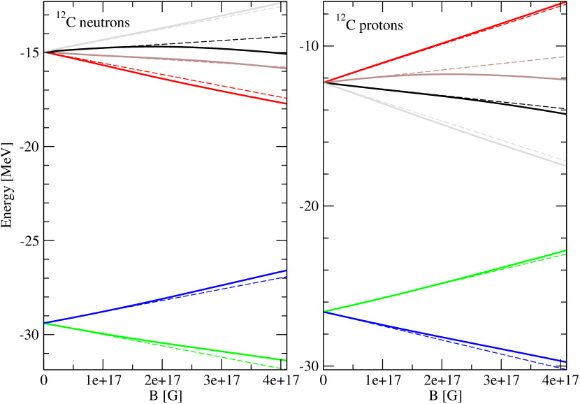
Figure 2.4: The energy levels (analytical (dashed) and numerical (solid)) as functions of the magnetic field for neutrons and protons in [12]C. The color code is analog to Figs. 2.2 and 2.3.

We have repeated the computations done for [16]O also for the nucleus [12]C. In Fig. 2.4 we present the energy levels. The difference between the analytical and the numerical results is much greater in this case compared to the [16]O nucleus.

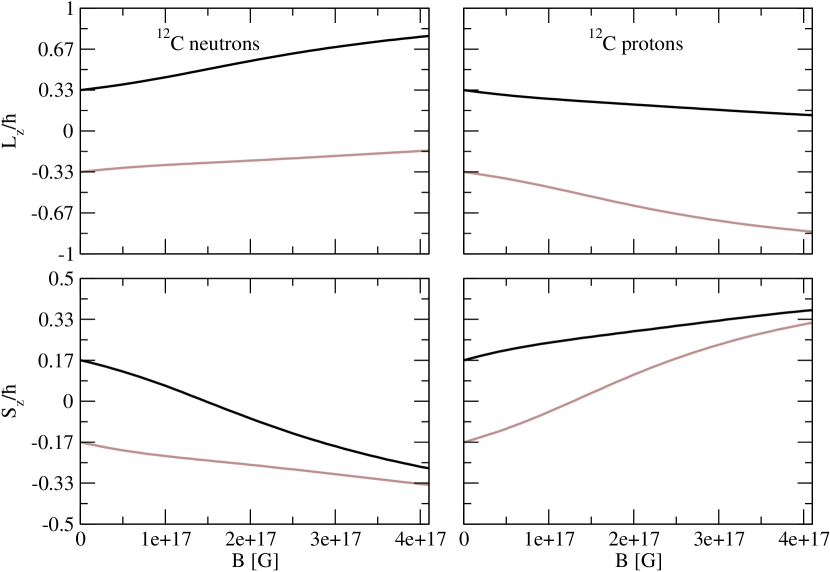
Figure 2.5: The angular momentum $\left<L_{z}\right>$ and the spin $\left<S_{z}\right>$ as functions of the magnetic field for neutrons and protons in [12]C. The color code is analog to Figs. 2.2 and 2.3.

In Fig. 2.5 we show only those $\left<L_{z}\right>/\hbar$ and $\left<S_{z}\right>/\hbar$ components of [12]C which differ from (half-)integer values. These are again those with mixed Clebsch-Gordan coefficients. They behave in the same way as those of [16]O.

The shape of the nucleus does not change much. At $B=0$, it is spherical symmetric with $r_{\mathrm{rms}}=2.47\,$fm, increasing slightly to 2.51 fm for $B_{\isotope[12]{C},\,e}=4.1\cdot 10^{17}\,$G which is defined in analogy to $B_{\isotope[16]{O},\,e}$. Increasing the magnetic field also results in a smooth deformation from $\beta=0$ at $B=0$ to $\beta=0.071$ at $B=B_{\isotope[12]{C},\,e}$. The deformation is always oblate with $\gamma=60\degree$.

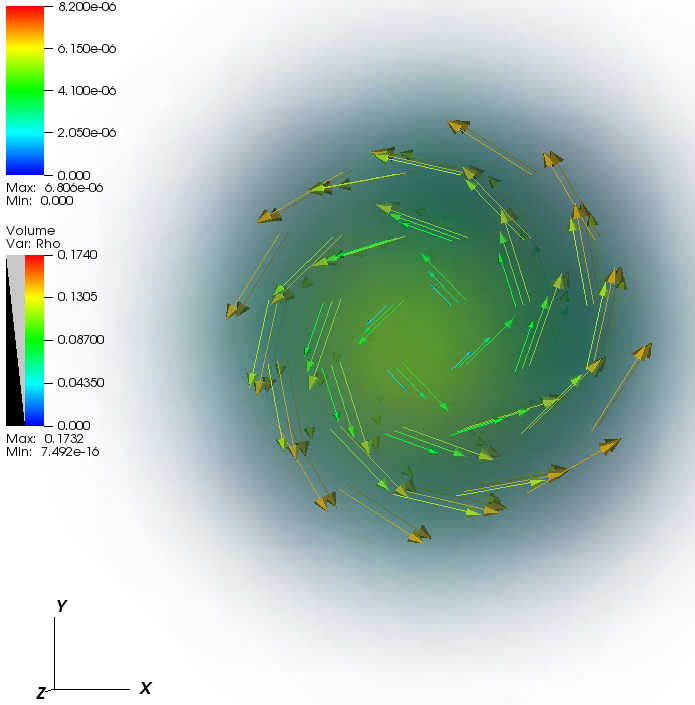
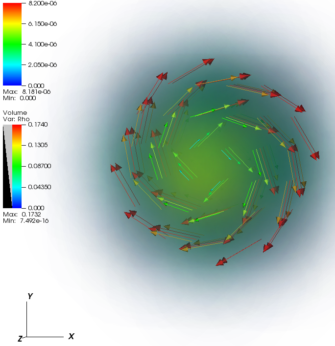
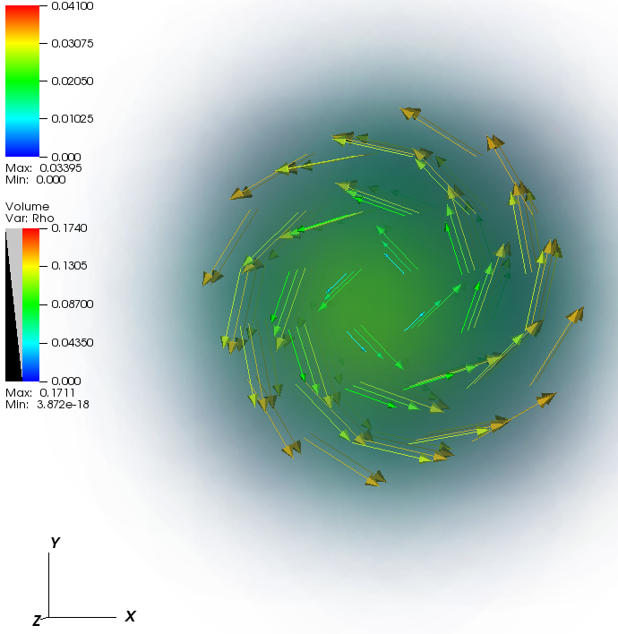
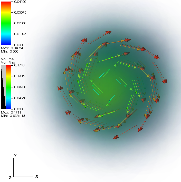
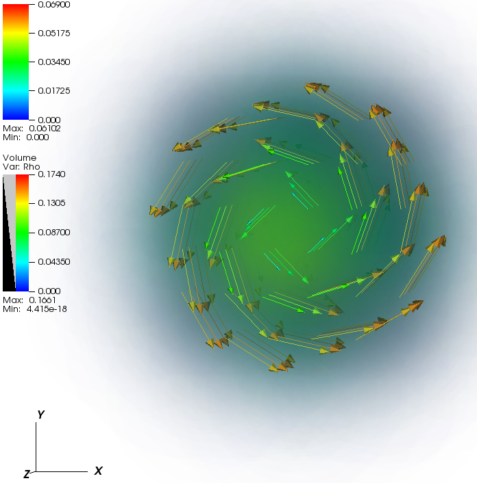
Figure 2.10: The current density divided by the particle density (collective flow velocity) for neutrons (left) and protons (right) for [12]C for different values of the magnetic field. Top: $B=4.0\cdot 10^{13}\,$G, middle: $B=2.0\cdot 10^{17}\,$G, bottom: $B=4.1\cdot 10^{17}\,$G. As background the particle density is added. This figure was created with VisIt [51].

We also evaluated the current and spin densities in Figs. 2.10 and 2.11 analogously to [16]O. We chose three magnetic fields. An infinitesimal magnetic field, $B_{i}=4.0\cdot 10^{13}\,$G, $B_{\isotope[12]{C},\,h}=2.0\cdot 10^{17}\,$G and $B_{\isotope[12]{C},\,e}$. Hereby $B_{\isotope[12]{C},\,h}\approx 1/2\cdot B_{\isotope[12]{C},\,e}$. $B_{i}$ is large enough for an orientation on the magnetic field, but too small to have other significant effects. For both quantities, the absolute values are approximately equal at each magnetic field for protons and neutrons, but the direction is opposite. The values increase with increasing magnetic field. We see that the current is concentrated at the surface for neutrons and protons, as we obtained for the protons of [16]O. For the spin we clearly see the change from the Zeeman effect to the Paschen-Back effect: For weak magnetic fields the l-s coupling is dominant, whereas for strong magnetic fields the spin is aligned with the $z$-axis.

To summarize, the [12]C nucleus in a magnetic field behaves similarly to [16]O for $B<B_{\isotope[16]{O},\,c}$. We do not find any redistribution of energy states in this case up to the strongest converging magnetic field. However, we expect redistributions to occur also for [12]C. For [12]C we find a similar behavior as for [16]O regarding the energy levels and the $z$-components of the s.p. angular momentum and spin. The alignment of spin density was more pronounced for [12]C than for [16]O.

Effects of the magnetic field on [20]Ne

Among the nuclei considered in this study ([12]C, [16]O and [20]Ne) the nucleus [20]Ne is the one which is farthest away from the closed shell structure. Indeed, [16]O is a double magic nucleus which has all $1s$ and $1p$ states filled. The [12]C is also a nucleus which has all $1s$ and all $1p_{3/2}$ states filled. If the states are filled according to the harmonic oscillator, in addition to the $1s$ and $1p$ states two $1d_{5/2}$ states should be filled in the case of [20]Ne nucleus.

We do not find states with half-integer numbers for $(\left<L_{z}\right>+\left<S_{z}\right>)/\hbar$. This nucleus is deformed and the symmetry axis of the nucleus is not equal to the axis of the magnetic field. Therefore the $z$-components are not good quantum numbers. Since we have no good quantum numbers for the $(\left<L_{z}\right>+\left<S_{z}\right>)/\hbar$ states, we do not present energy states and $\left<L_{z}\right>$ and $\left<S_{z}\right>$ for [20]Ne in contrast to the evaluation of the other nuclei.

In contrast to [16]O, we do not have two sectors, but we have continuous deformations as smooth functions of the magnetic field. As for [16]O, we regard $r_{\mathrm{rms}}$, $\beta$ and $\gamma$ for evaluating the size and shape of the nucleus, see Figs. 2.6 and 2.7. Fig. 2.7 was created with VisIt [51]. Fig. 2.6 shows some parameters as functions of the magnetic fields. Fig. 2.7 shows the deformed nucleus for $B=0$, $B_{\isotope[20]{Ne},\,h}=2.4\cdot 10^{17}\,$G and $B_{\isotope[20]{Ne},\,e}=4.9\cdot 10^{17}\,$G, hereby $B_{\isotope[20]{Ne},\,h}$ and $B_{\isotope[20]{Ne},\,e}$ are defined in analogy to $B_{\isotope[12]{C},\,h}$ and $B_{\isotope[12]{C},\,e}$. The radius $r_{\mathrm{rms}}$ slightly decreases from 2.93 fm to 2.87 fm. However, $\beta$ decreases from 0.32 to 0.15 to a value being less than half of the original one. This denotes a continuous significant change in the deformation, which can be seen well in Figs. 2.6 and 2.7. $\gamma$ starts at $0\degree$ for $B=0$, but increases asymptotically to $11\degree$, denoting a change from a purely prolate deformed nucleus to a mainly prolate deformed one.

Analogously to [12]C we evaluated the current and spin densities in Figs. 2.12 and 2.13 for $B_{i}$, $B_{\isotope[20]{Ne},\,h}$ and $B_{\isotope[20]{Ne},\,e}$. Apart from the current at infinitesimal magnetic field, the absolute values of both quantities are again approximately equal at each magnetic field for protons and neutrons and the direction is again opposite. The values increase with increasing magnetic field. Again the current is concentrated at the surface. The change from the Zeeman effect to the Paschen-Back effect is again clearly seen in the spin. However, in this highly deformed nucleus, we see two main axis for spin alignment. In all figures concerning [20]Ne, we see a stronger change of values at weaker magnetic fields, explaining why figures for $B_{\isotope[20]{Ne},\,h}$ look more similar to those of $B_{\isotope[20]{Ne},\,e}$ than to those of $B=0$ or $B_{i}$.

The current distribution could give a clearer understanding of the deformation. At vanishing magnetic field, the nucleus is deformed with nucleons at low velocity. Increasing the magnetic field increases the collective flow velocity. Hence the orbits of the nuclei approach to circular orbits resulting in a less deformed nucleus at stronger magnetic fields.

Accuracy considerations

The code Sky3D offers several variables for judging the convergence. E.g. the average uncertainties in the single particle energies $\Delta\varepsilon_{1}$ and $\Delta\varepsilon_{2}$ defined as

$$\Delta\varepsilon_{1} = \sqrt{\left<\psi\middle|\hat{h}^{2}\middle|\psi\right>-\left<\psi\middle|\hat{h}\middle|\psi\right>^{2}}\,,$$ (2.20a)

$$\Delta\varepsilon_{2} = \sqrt{\left<\hat{h}\psi\middle|\hat{h}\psi\right>-\left<\psi\middle|\hat{h}\middle|\psi\right>^{2}}\,.$$ (2.20b)

These uncertainties have to be low. Moreover, the change in the total energy has to be low, but the uncertainties of Eq. (2.20) are more important [50].

For all results of this chapter, we obtain $\Delta\varepsilon_{1}<10^{-3}$ and $\Delta\varepsilon_{2}<10^{-3}$. For [16]O we obtain $\Delta\varepsilon_{1}<10^{-4}$ and $\Delta\varepsilon_{2}<10^{-4}$ for $B<B_{\isotope[16]{O},\,c}$. For [12]C we obtain $\Delta\varepsilon_{1}<10^{-4}$ and $\Delta\varepsilon_{2}<10^{-4}$ for $B\leq 2.9\cdot 10^{17}\,$G. For all results of this chapter we obtain $\Delta\varepsilon_{2}<10^{-4}$ for [12]C, whereas $\Delta\varepsilon_{1}$ increases above $10^{-4}$.

2.3.4 Outlook

To achieve convergence on strong magnetic fields, we used several methods, explained in 2.3.3. Hereby we improved the convergence and got the results presented in this chapter. Besides these techniques, we changed the Skyrme force and we introduced the spin-spin term in the Hamiltonian analogue to [49]. However, these attempts were not yet successful. For future works, it will be interesting to develop all these techniques and to study effects for strengths of the magnetic field where our present methods fail to converge. In addition, it will be interesting to study nuclei which are likely to occur in magnetars, the nuclei we studied for this work are not likely to occur in magnetars [46]. Moreover, it will be interesting to study the effects of the magnetic field on different terms of the Hamiltonian, which we neglected, e.g. the spin-spin interaction.

Figure 2.1: The quantum numbers for different states. The orbital angular momentum and spin of states are given by these quantum numbers or by superpositions of them. The limit of weak magnetic fields can be seen in Eq. (2.10), for increasing magnetic field the prefactors of the mixed states differ. The limit of strong magnetic fields can be seen in Eq. (2.19).

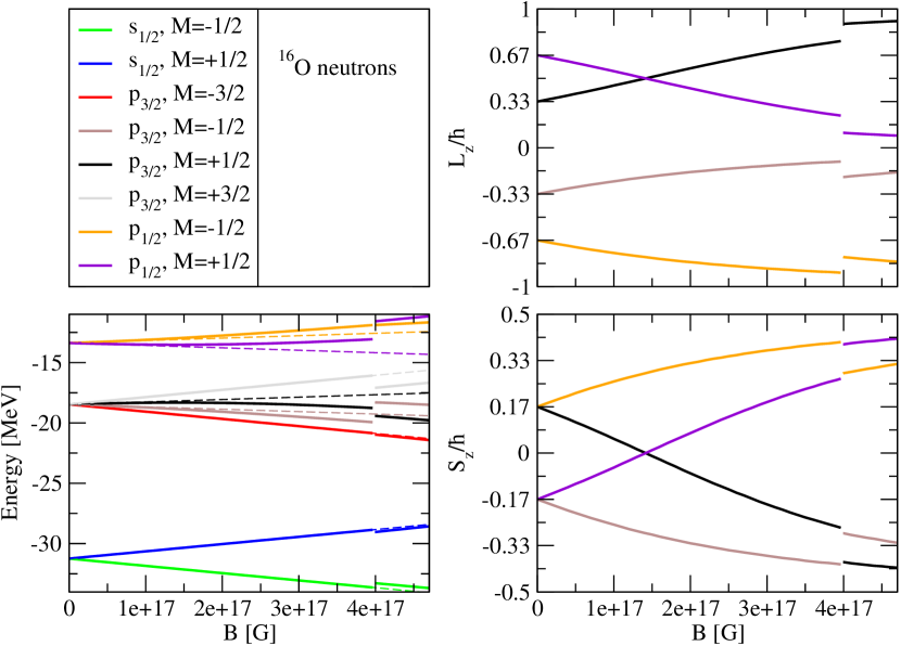
Figure 2.3: The energy levels (analytical (dashed) and numerical (solid)), $\left<L_{z}\right>$ and $\left<S_{z}\right>$ as functions of the magnetic field for neutrons in [16]O.

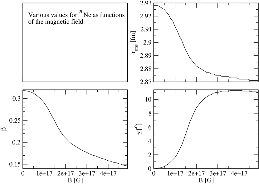
Figure 2.6: The $r_{\mathrm{rms}}$, $\beta$ and $\gamma$ as functions of the magnetic field for [20]Ne.

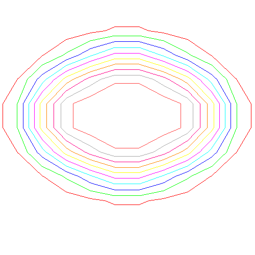
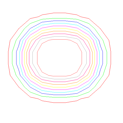
Figure 2.7: The deformed [20]Ne nucleus for $B=0$, $B=2.4\cdot 10^{17}\,$G and $B=4.9\cdot 10^{17}\,$G. This figure was created with VisIt [51].

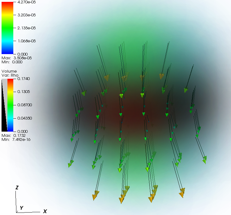
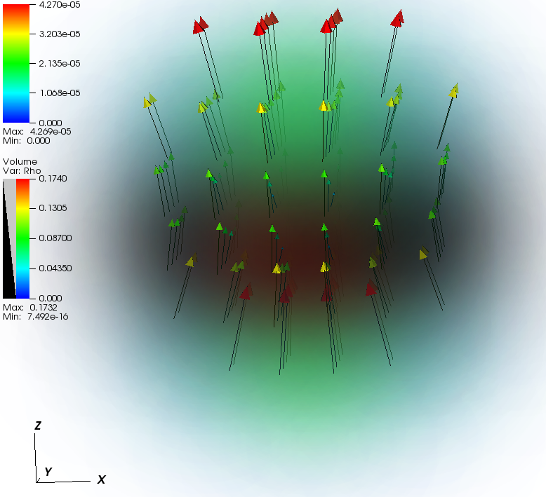
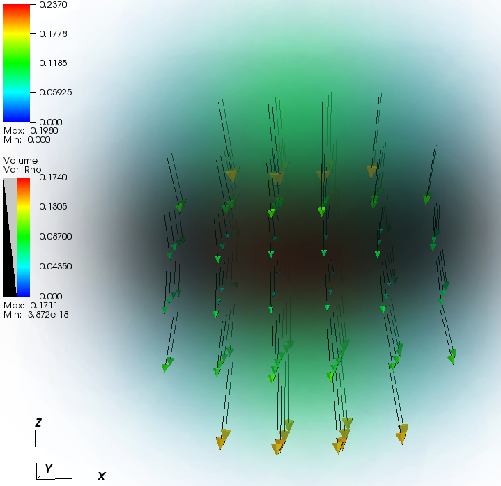
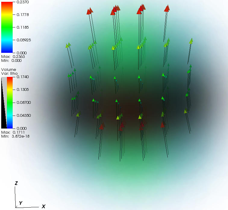
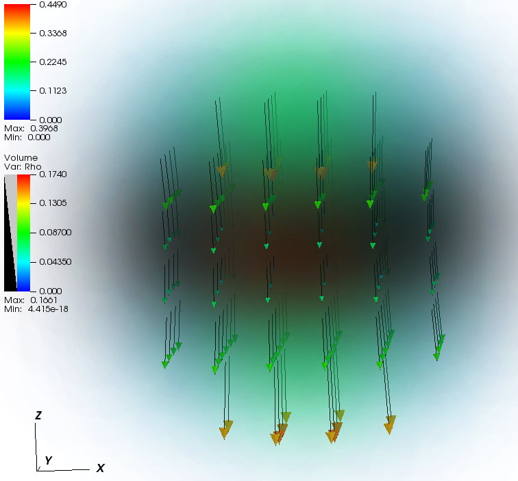
Figure 2.11: The spin density divided by the particle density for [12]C with the same arrangement and magnetic fields as in Fig. 2.10. This figure was created with VisIt [51].

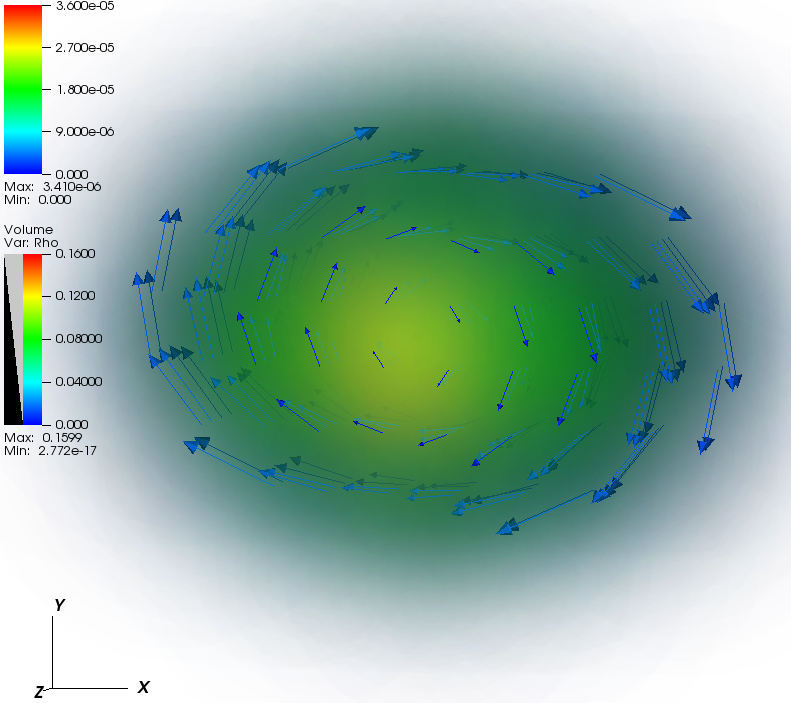
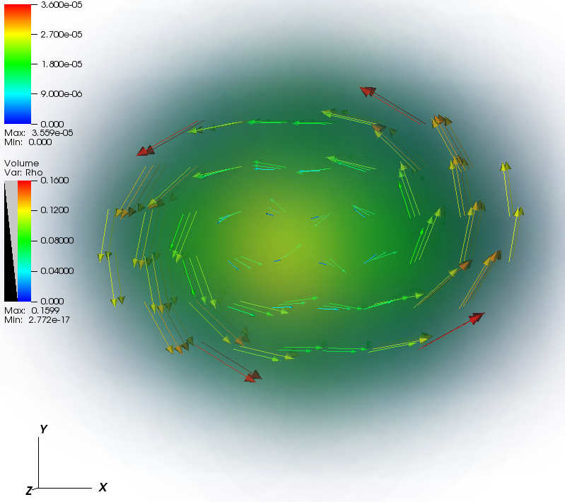
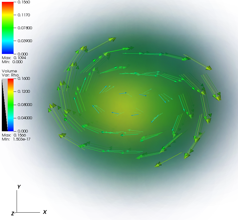
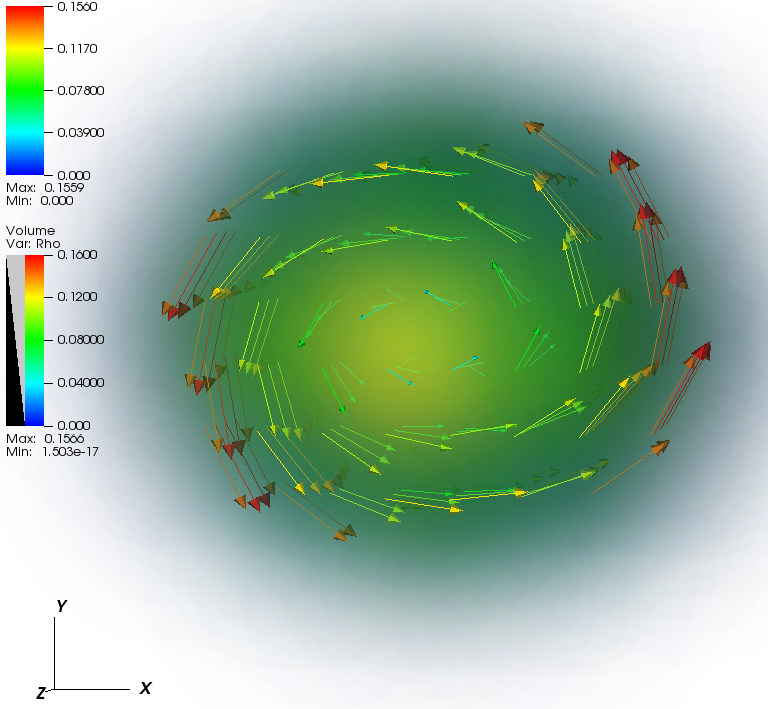
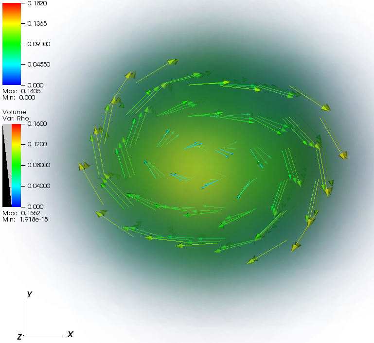
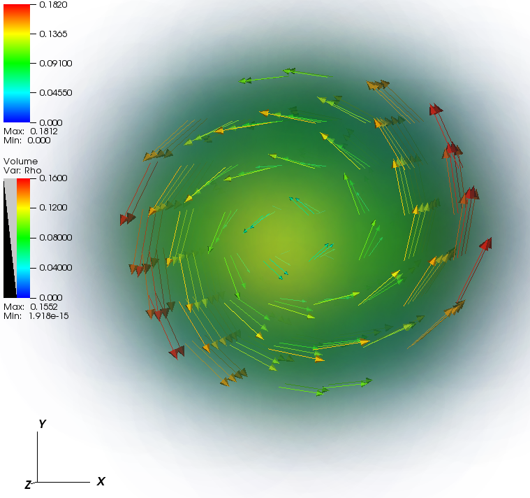
Figure 2.12: The current density divided by the particle density (collective flow velocity) for neutrons (left) and protons (right) for [20]Ne for different values of the magnetic field. Top: $B=4.0\cdot 10^{13}\,$G, middle: $B=2.4\cdot 10^{17}\,$G, bottom: $B=4.9\cdot 10^{17}\,$G. As background the particle density is added. This figure was created with VisIt [51].

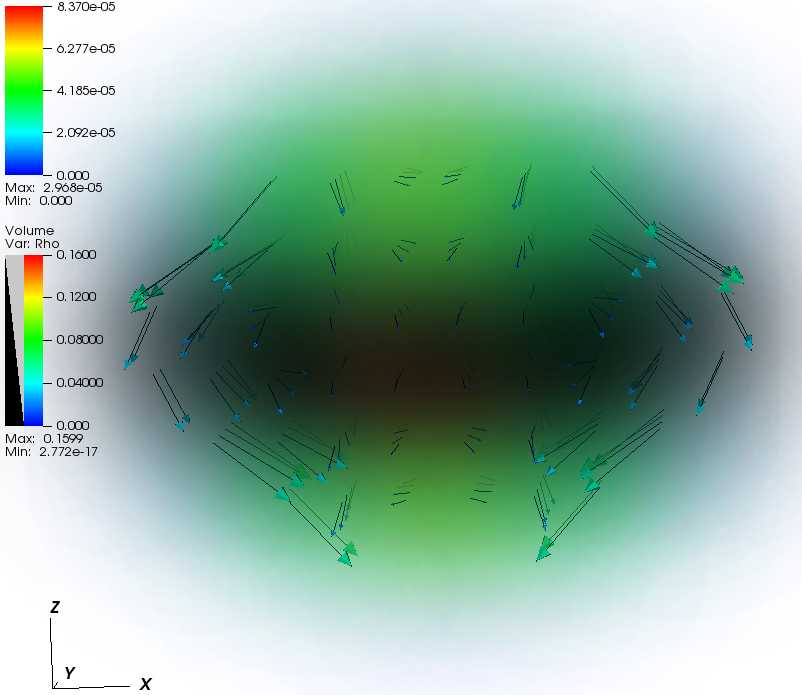
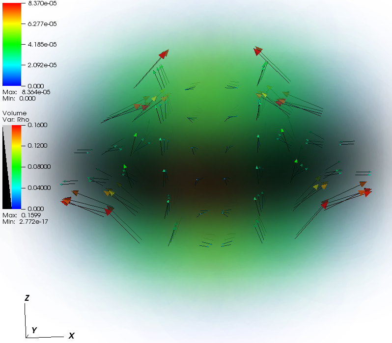
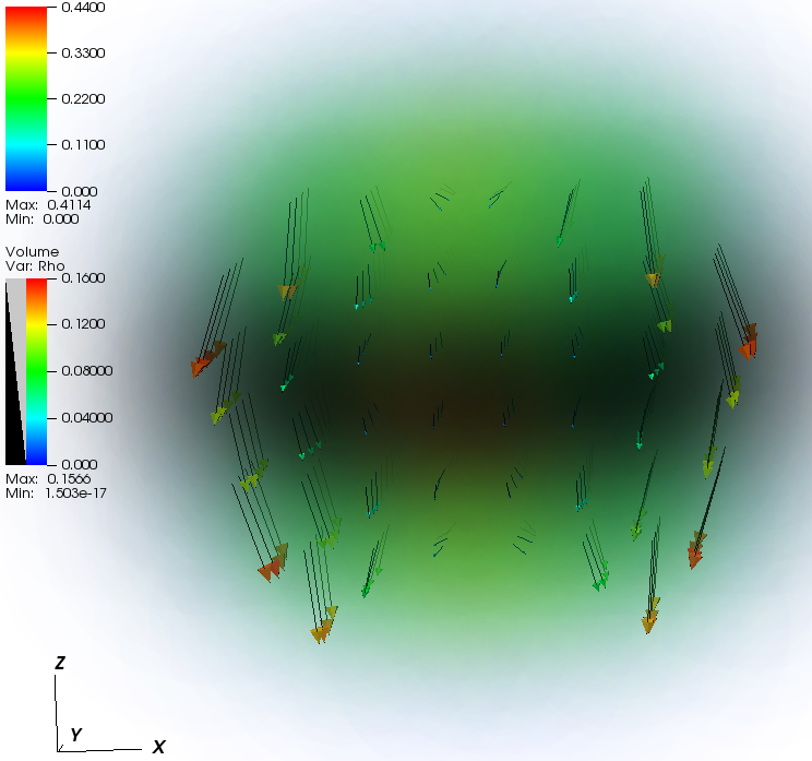
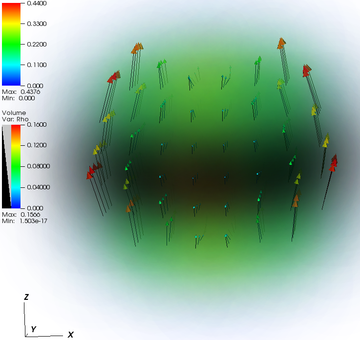
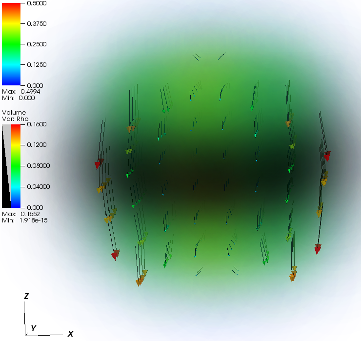
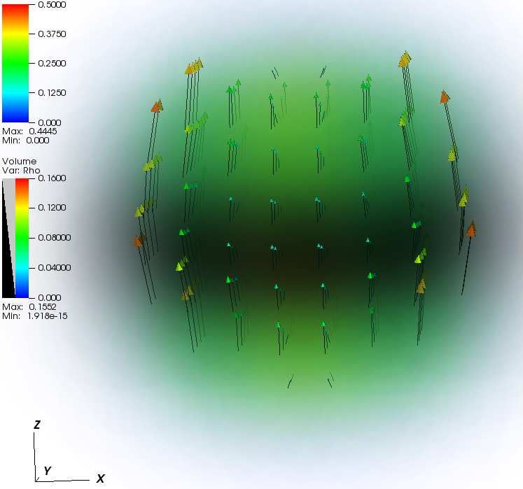
Figure 2.13: The spin density divided by the particle density for [20]Ne with the same arrangement and magnetic fields as in Fig. 2.12. This figure was created with VisIt [51].

2.4 Conclusion

We have studied the effects of strong magnetic fields on different nuclei using a Skyrme-Hartree-Fock (SHF) approach [49, 50] calculated with the code Sky3D [50]. The strong magnetic fields can be realized e.g. in neutron stars [42, 43, 44, 45]. The elements we study occur in white dwarfs [48], which also have strong magnetic fields [47].

We studied the effects of strong magnetic fields on different nuclei and our results can be summarized as follows:

• [16]O is a double magic nucleus. For $B<B_{\isotope[16]{O},\,c}$ it has the lowest states of the harmonic oscillator filled and it is spherical symmetric. We find a change from a Zeeman effect to a Paschen-Back effect dominated region by increasing the magnetic field. For magnetic fields above $B_{\isotope[16]{O},\,c}$, we find a rearrangement of energy states and a slight deformation of the nucleus. The current and spin densities of neutrons and protons differ a lot above $B_{\isotope[16]{O},\,c}$.

• [12]C is an isospin symmetric nucleus which is in many ways analogous to [16]O. Also the lowest states of the harmonic oscillator are filled and the change from a Zeeman effect to a Paschen-Back effect dominated region is clearly seen. The current and spin densities of neutrons and protons differ in direction but not much in magnitude.

• [20]Ne is an isospin symmetric nucleus. At vanishing magnetic field it is strongly deformed in a purely prolate deformation. Increasing the magnetic field decreases the strength of the deformation and changes the shape from purely prolate to mainly prolate. In general we obtain equal features for current and spin densities as for [12]C, but due to the deformation it shows more interesting features.

Future work may extend the present studies in different directions, in particular as follows:

• An improved Hamiltonian can be considered. In particular including the spin-spin interaction may be interesting in the context of strong magnetic fields.

• Extension of the present studies to stronger magnetic fields. For that purpose the techniques which have been used in this study must be improved or modified.

Chapter 3 BCS pairing in neutron matter

3.1 Introduction

In this chapter we continue the discussion of pairing in nuclear systems, started in chapter 1. In particular, we study here the pairing in pure neutron matter in strong magnetic fields (strong magnetic fields we have already discussed in chapter 2). The order of magnitude of these fields is within the range $10^{16}-10^{17}$ G, which was also relevant for our discussion of nuclei in the previous chapter. We will show the analogies between isospin asymmetric pairing in neutron-proton systems and spin-polarized (spin asymmetric) neutron matter and contrast them by pointing out the key differences.

Neutron-neutron pairing was studied extensively in the past, see for example [11, 12, 13, 14, 15, 16, 17]. Neutron-neutron pairing comes into play in systems where the isospin asymmetry is large enough to suppress the dominant ${}^{3}S_{1}$-${}^{3}D_{1}$ pairing. The isospin triplet pairing in the ${}^{3}S_{1}$-${}^{3}D_{1}$ channel is prohibited by Pauli blocking in pure neutron matter. Therefore, the dominant pairing channel is an isospin singlet state, which at low-energies (low-densities) is in the ${}^{1}S_{0}$ channel. We may then expect that a spin-polarization, e.g., induced by a magnetic field will suppress the pairing significantly. At large energies (high densities) the dominant pairing channel in neutron matter is the ${}^{3}P_{2}$-${}^{3}F_{2}$ pairing channel, which corresponds to a spin-1 condensate of neutrons [17]. In this case the spin-polarizing effect of the magnetic field on the internal structure of the spin-1 pairs is non-destructive.

Because in the vacuum the two-neutron system is unbound, diluting neutron matter does not lead automatically to a state with strongly bound two-neutron gas, which may then form a Bose condensate. Therefore, in general one cannot expect a Bose condensed regime of neutron-pairs in the low-density limit [11]. Nevertheless, as shown in Refs [13, 14, 11] a BCS-BEC crossover region may exist also for neutron matter, when the neutron matter is diluted. This, in principle, occurs in full analogy with the ${}^{3}S_{1}$-${}^{3}D_{1}$ pairing, with the exception that the asymptotical state of the system at low-densities is non-interacting neutron gas, instead of a Bose condensate of neutron-pairs.

In a first approximation neutron star matter can be treated as pure neutron matter [16], because the fraction of protons and electrons (and other heavier baryons) does not exceed $5\%$-$10\%$ of the total density of the system. Thus, it is well known that neutron-neutron pairing plays an important role in the physics of the inner crust of a neutron star. It plays also a significant role for neutron-rich nuclei near the drip line [13]. This type of pairing may also occur for halo neutrons in halo nuclei, such as, e.g. ¹¹Li [13]. There are some phenomenological indications of neutron superfluidity in neutron stars. Prominent examples are glitches in the rotational behavior of some pulsars, as well as the cooling behavior of the youngest known neutron star in Cassiopeia A [17].

3.2 Theory

In this section we adapt the formalism developed in chapter 1 to the case of neutron matter. We will continue to use the separable version of the Paris potential. However, now we would like to extend the discussion to arbitrary rank $n$ separable potentials. This extension applies for both uncoupled channels, such as the ${}^{1}S_{0}$ channel as well as for coupled channels as the ${}^{3}S_{1}$-${}^{3}D_{1}$ channel.

We start with some basic definition following Ref. [75]. The gap equation for an uncoupled neutron-neutron channel can be written as

$$\Delta_{l}({\bm{k}})=\sum_{l^{\prime}}\int\frac{d^{3}k^{\prime}}{(2\pi)^{3}}V_{l,l^{\prime}}({\bm{k}},{\bm{k}}^{\prime})\phi_{l^{\prime}}({\bm{k}}^{\prime})\,,$$ (3.1)

where we use the same notations as in chapter 1 and we define

$$\phi_{l}({\bm{k}})=\frac{1}{4}\sum_{a,r}\frac{\Delta_{l}({\bm{k}})}{2\sqrt{E_{S}^{2}({\bm{k}})+\Delta^{2}({\bm{k}})}}[1-2f(E^{a}_{r}({\bm{k}})]\,.$$ (3.2)

Here the neutron spin-up and spin-down spectra are given by

$$E_{r}^{a} = \sqrt{E_{S}^{2}+\Delta^{2}}+r\delta\mu+aE_{A}\,,$$ (3.3)

where

$$E_{S}=\left(Q^{2}/4+k^{2}\right)/2m^{*}-\bar{\mu}\,,\qquad E_{A}={\bm{k}}\cdot{\bm{Q}}/2m^{*}\,,$$ (3.4)

and

$$\delta\mu=\tfrac{1}{2}(\mu_{\uparrow}-\mu_{\downarrow})\,,\qquad\bar{\mu}=\tfrac{1}{2}(\mu_{\uparrow}+\mu_{\downarrow})\,,$$ (3.5)

where $\delta\mu$ describes the spin-polarization of neutron matter in terms of chemical potentials of spin-up $\mu_{\uparrow}$ and spin-down $\mu_{\downarrow}$ chemical potentials. The symmetric part of the spectrum $E_{S}$ contains a kinetic energy shift due to the finite momentum and an “averaged” chemical potential $\bar{\mu}$. The angle-dependent part of the spectrum $E_{A}$ is the kinematical factor that allows for LOFF phase. It describes the mutual shift in the Fermi-surfaces of spin-up and spin-down neutrons which allows for partial overlap of the Fermi-surfaces at the cost of additional kinetic energy appearing in $E_{S}$. Thus we see that for $\delta\mu=0$ one recovers the spin-unpolarized limit, whereas for $E_{A}=0$ the LOFF phase is excluded from consideration.

The condensation energy of neutron matter is given by

$$E_{\mathrm{cond}}= \frac{g_{\mathrm{deg}}}{2}N_{\Omega}\sum_{l,l^{\prime}}\int\frac{d^{3}k}{(2\pi)^{3}}\int\frac{d^{3}k^{\prime}}{(2\pi)^{3}}V_{l,l^{\prime}}({\bm{k}},{\bm{k}}^{\prime})\phi_{l}({\bm{k}})\phi_{l^{\prime}}({\bm{k}}^{\prime})\,,$$ (3.6)

where $g_{\mathrm{deg}}$ is the degeneration factor; $g_{\mathrm{deg}}=2$ for neutron matter and $g_{\mathrm{deg}}=4$ for symmetric nuclear matter. $N_{\Omega}$ is the gap averaging factor. For the ${}^{1}S_{0}$ pairing channel we obtain $N_{\Omega}=1$. For the ${}^{3}S_{1}$-${}^{3}D_{1}$ pairing channel, which can occur e.g. for neutron-proton pairing, we obtain $N_{\Omega}=3/(8\pi)$.

It will be convenient in the following to describe the polarization of matter also in terms of the partial densities of spin-up and spin-down particles

$$\alpha=\frac{\rho_{\uparrow}-\rho_{\downarrow}}{\rho_{\uparrow}+\rho_{\downarrow}}\,.$$ (3.7)

Finally, we note that we use the same Skyrme functional based expression for the effective mass of neutrons as was used in chapter 1

$$\frac{m}{m^{*}} = \left[1+\frac{\rho\cdot m}{8\hbar^{2}}(3t_{1}+5t_{2})\right]\,.$$ (3.8)

We will neglect the effects of spin-polarization on the effective mass of neutrons. This is a small effect compared to the ones that are taken into account (i.e. the splitting in the chemical potentials of spin-up and down particles.)

Now we proceed to implement a separable potential in the preceding equations. Following Ref. [20] we define a separable potential as

$$V_{l,l^{\prime}}(k,k^{\prime})=-2\pi^{2}\sum_{i=1}^{n}\sum_{j=1}^{n}\lambda_{ij}\cdot g_{li}(k)g_{l^{\prime}j}(k^{\prime})\,.$$ (3.9)

To solve the gap equation we carry out angle averaging in the denominator of the gap equation by substituting

$$\Delta^{2}(k) = N_{\Omega}\sum_{l}\Delta_{l}^{2}(k)\,.$$ (3.10)

The separable potential allows one to make the following ansatz for the gap function

$$\Delta_{l}(k) = \sum_{i=1}^{n}c_{i}\cdot g_{li}(k)\,,$$ (3.11)

where $c_{i}$ are constants. Then the gap equation takes the form

$$\sum_{i=1}^{n}c_{i}\cdot g_{li}(k) = -2\pi^{2}\cdot\frac{1}{4}\sum_{a,r}\sum_{l^{\prime}}\sum_{i=1}^{n}g_{li}(k)\sum_{j=1}^{n}\lambda_{ij}\int\frac{d^{3}k^{\prime}}{(2\pi)^{3}}g_{l^{\prime}j}(k^{\prime})$$

$$\times\frac{\Delta_{l^{\prime}}(k^{\prime})}{2\sqrt{E_{S}^{2}(k^{\prime})+\Delta^{2}(k^{\prime})}}\cdot[1-2f(E^{a}_{r}(k^{\prime}))]\,.$$

This equation will be fulfilled for arbitrary sets of functions $g_{li}(k)$ only if for each term in the $i$ sum we have

$$c_{i} = -2\pi^{2}\cdot\frac{1}{4}\sum_{a,r}\sum_{l}\sum_{j=1}^{n}\lambda_{ij}\int\frac{d^{3}k}{(2\pi)^{3}}g_{lj}(k)\newline$$

$$\times\frac{\Delta_{l}(k)}{2\sqrt{E_{S}^{2}(k)+\Delta^{2}(k)}}\cdot[1-2f(E^{a}_{r}(k))]$$

$$= -2\pi^{2}\sum_{l}\sum_{j=1}^{n}\lambda_{ij}\int\frac{d^{3}k}{(2\pi)^{3}}g_{lj}(k)\phi_{l}(k)\,.$$ (3.13)

Thus the problem reduces to solving a set of non-linear algebraic equations.

In the following step we compute the condensation energy for separable interactions. For that purpose with insert Eq. (3.1) in Eq. (3.6) and find

$$E_{\mathrm{cond}} = \frac{g_{\mathrm{deg}}}{2}N_{\Omega}\sum_{l}\int\frac{d^{3}k}{(2\pi)^{3}}\Delta_{l}(k)\phi_{l}(k)\,.$$ (3.14)

For a rank 1 potential we obtain the solution of the gap equation as

$$c = -2\pi^{2}\sum_{l}\lambda\int\frac{d^{3}k}{(2\pi)^{3}}g_{l}(k)\phi_{l}(k)\,,\qquad\Delta_{l}(k)=c\cdot g_{l}(k)\,.$$ (3.15)

The condensation energy is then given in terms of the $c$-coefficient

$$E_{\mathrm{cond}} = \frac{g_{\mathrm{deg}}}{2}\cdot\frac{N_{\Omega}\cdot c}{\lambda}\sum_{l}\lambda\int\frac{d^{3}k}{(2\pi)^{3}}g_{l}(k)\phi_{l}(k)$$ (3.16)

$$= -\frac{g_{\mathrm{deg}}}{2}\cdot\frac{N_{\Omega}\cdot c^{2}}{2\pi^{2}\cdot\lambda}\,.$$

In analogy to Eq. (1.45) we can define the grand canonical potential as

$$\Omega(\Delta,{\bm{Q}}) = \frac{g_{\mathrm{deg}}}{2}N_{\Omega}\sum_{l}\int\frac{d^{3}k}{(2\pi)^{3}}\Delta_{l}({\bm{k}})\phi_{l}({\bm{k}})$$ (3.17)

$$-\frac{g_{\mathrm{deg}}}{4}\sum_{a,r}\int\frac{d^{3}k}{(2\pi)^{3}}\left[\frac{E^{a}_{r}({\bm{k}})-E_{S}({\bm{k}})}{2}\right.$$

$$+\left.T\ln\left(1+e^{-\beta E^{a}_{r}({\bm{k}})}\right)\right]$$

and in analogy to Eq. (1.48) we can define

$$\tilde{\Omega}(\Delta,{\bm{Q}}) = \Omega(\Delta,{\bm{Q}})-\Omega(0,{\bm{Q}})+\Omega(0,0)\,.$$ (3.18)

In analogy to Eq. (1.49) the associated free energy of the system is given by

$$F(\Delta,{\bm{Q}}) = \tilde{\Omega}(\Delta,{\bm{Q}})+\mu_{\uparrow}\rho_{\uparrow}+\mu_{\downarrow}\rho_{\downarrow}\,.$$ (3.19)

To complete our set of equations, we define the densities of the spin-up and down particles in analogy to the densities of neutrons and protons in chapter 1:

$$\rho_{\uparrow/\downarrow}({\bm{Q}}) = \frac{g_{\mathrm{deg}}}{4}\int\frac{d^{3}k}{(2\pi)^{3}}\cdot\left(1+\frac{E_{S}}{\sqrt{E_{S}^{2}+\Delta^{2}}}\right)f(E^{+}_{\mp})$$ (3.20)

$$+\left(1-\frac{E_{S}}{\sqrt{E_{S}^{2}+\Delta^{2}}}\right)(1-f(E^{-}_{\pm}))\,.$$

For the following discussion we also define the Fermi momenta of spin-up and down neutrons at zero temperature

$$k_{F\uparrow/\downarrow}=(6\pi^{2}\rho_{\uparrow/\downarrow})^{1/3}\,,$$ (3.21)

as well as the Fermi-momentum of unpolarized (spin-symmetrical) neutron matter

$$k_{F}=(3\pi^{2}\rho)^{1/3}\,,$$ (3.22)

where $\rho=\rho_{\uparrow}+\rho_{\downarrow}$ is the net density.

In closing of this section we related the spin-polarization to the magnetic field. Obviously,

$$\delta\mu=-\tilde{\mu}_{n}B\,,$$ (3.23)

where the minus sign is chosen to have positive $\delta\mu$ as in chapter 1 and

$$\tilde{\mu}_{n}=\frac{g_{n}}{2}\cdot\mu_{N}=\frac{g_{n}}{2}\cdot\frac{e\hbar}{2m^{*}c}\,,$$ (3.24)

where $g_{n}=-3.82608544$ is the neutron $g$-factor. We will sometimes use the energy scale that describes the spin-polarization

$$\varepsilon_{B}=|\delta\mu|=\left|\tilde{\mu}_{n}B\right|\,.$$ (3.25)

3.3 Results

Using strategies as in chapter 1 the phase diagram of spin-polarized neutron matter was calculated. The intrinsic features of spin-polarized matter were extracted at the points in the density-temperature diagram listed in Table 3.1. The computations were carried out with the rank-3 separable Paris potential (PEST 3) in the ${}^{1}S_{0}$ partial wave channel with parameters listed in Ref. [20]. We found that there exists neither LOFF phase nor BEC regime in spin-polarized neutron matter. The main reason for the absence of the LOFF phase is that the neutron condensate is more “fragile” than the neutron-proton condensate. Indeed the ratio of the gap to the chemical potential is by about factor 10 smaller in neutron matter, because for the same density the chemical potential is larger in pure neutron matter than in the symmetrical nuclear matter and at the same time the ${}^{1}S_{0}$ interaction is at all energies weaker than the ${}^{3}S_{1}$-${}^{3}D_{1}$ interaction. Furthermore, we ignored the possibility of a phase-separation in spin-polarized neutron matter. Finally, concerning the BCS-BEC crossover our findings are as follows. No change in the sign of the chemical potential was observed, i.e., the chemical potential had only positive values at the lowest density studied. The lowest value we checked was $\mu_{n}=0.24$ MeV for $\log(\rho/\rho_{0})=-3.57$, $T=0.05$ MeV in spin-symmetric neutron matter. This point is located at the transition line to the unpaired phase. This indicates a vanishing chemical potential at the low density vanishing temperature transition. The reason that we do not find clear BEC condensate of neutron pairs is that the no bound neutron-neutron pairs are supported in the vacuum by the nuclear interaction. However, it should be noted that although the chemical potential does not change its sign, we find that $d/\xi_{a}\ll 1$ at high density and $d/\xi_{a}\geq 1$ at low-densities, which is an indication of a BEC precursor.

In Table 3.1 (which is similar to Table 1.1) we present several quantities of interest for three different values for the density at $T=0.25$ MeV at vanishing spin-polarization. The above indicated behavior of the ratio $d/\xi_{a}$ is demonstrated.

log$\left(\frac{\rho}{\rho_{0}}\right)$	$k_{F}$ [fm-1]	$\Delta$ [MeV]	$m^{\ast}/m$	$\mu_{n}$ [MeV]	$d$ [fm]	$\xi_{\rm rms}$ [fm]	$\xi_{a}$ [fm]
$-1.0$	0.78	2.46	0.967	12.94	2.46	4.87	4.33
$-1.5$	0.53	1.91	0.989	5.65	3.61	3.55	3.71
$-2.0$	0.36	1.07	0.997	2.49	5.30	2.36	4.48

Table 3.1: The table shows the net density $\rho$ (in units of nuclear saturation density $\rho_{0}=0.16$ fm^-3), Fermi momentum $k_{F}$, gap $\Delta$, effective mass (in units of bare mass), chemical potential $\mu_{n}$, interparticle distance $d$, and coherence lengths $\xi_{\rm rms}$ and $\xi_{a}$ in unpolarized neutron matter at fixed $T=0.25$ MeV. The pairing is in the ${}^{1}S_{0}$ channel.

3.3.1 Phase diagram

The phase diagram was computed by solving Eqs. (3.1) and (3.20) self-consistently for pairing in the ${}^{1}S_{0}$ channel. These equations are analogous to Eqs. (1.42) and (1.44). The LOFF phase was searched for by varying the Cooper-pair momentum ${\bm{Q}}$ in Eq. (3.19) and by looking at the minimum of the free energy. It was found that in the parameter range considered the minimum was always at ${\bm{Q}}=0$. The reason for this, as explained above, is the “weakness” of the neutron pairing compared to the neutron-proton pairing.

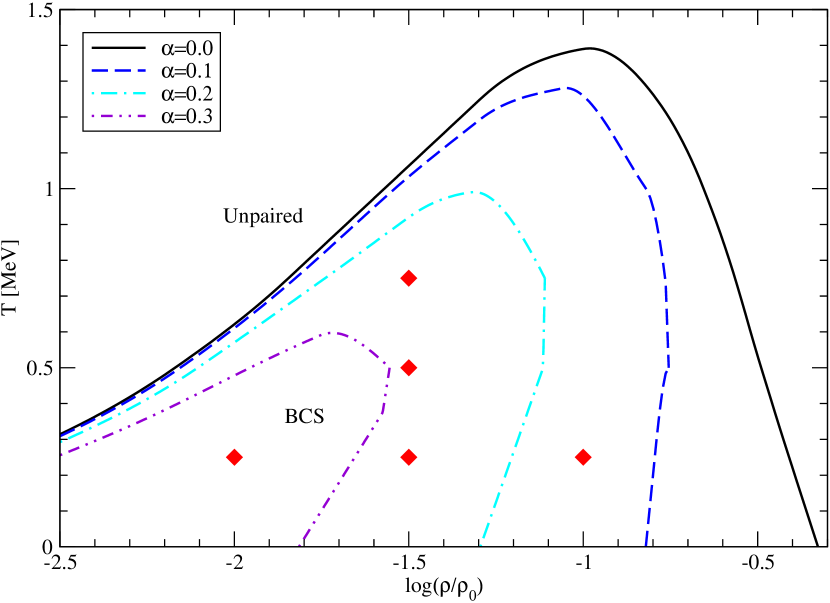
Figure 3.1: Phase diagram of neutron matter in the temperature-density plane for several spin-polarizations $\alpha$, induced by magnetic fields. Included are the BCS and the unpaired phase. The red diamonds refer to different points in the phase diagram at which we evaluated some intrinsic features. This figure is analog to Fig. 1.2.

The resulting phase diagram of neutron matter is shown in Fig. 3.1. It only consists of the BCS and the unpaired phases. In general we obtain the same structure as in the case of nuclear matter shown in Fig. 1.2. At low densities the critical temperature increases with increasing density, for high densities it decreases. This shape results from Eqs. (1.57) and (1.58), see discussion in subsection 1.3.1. The polarization suppresses the pairing efficiently only for high densities.

The phase diagram of spin-polarized neutron matter is less complex because no exotic phase are present. However, an interesting feature seen in the diagram is that the transition line to the unpaired phase is not a single-valued function of the density in a range of densities. The reason is well understood: at low temperature the matter is in the unpaired phase by small separation of the Fermi spheres as the thermal smearing of the Fermi-surfaces is ineffective to produce phase-space overlap. Increasing the temperature at fixed density and polarization makes the smearing of the Fermi surfaces more effective resulting in an overlap and thus a restoration of the BCS phase (see subsections 1.3.3 and 1.3.2 for further discussion).

3.3.2 Intrinsic features

We now proceed to study some intrinsic features of the isospin-triplet ${}^{1}S_{0}$ neutron condensate, as was done for the ${}^{3}S_{1}$-${}^{3}D_{1}$ condensate in chapter 1. Because there are many similarities in the relevant quantities (such as the pairing gap, the kernel, the wave functions, the occupation numbers and the quasiparticle spectrum) we will not carry out a complete discussion. We will try to point out the main differences and the most prominent features.

The Gap

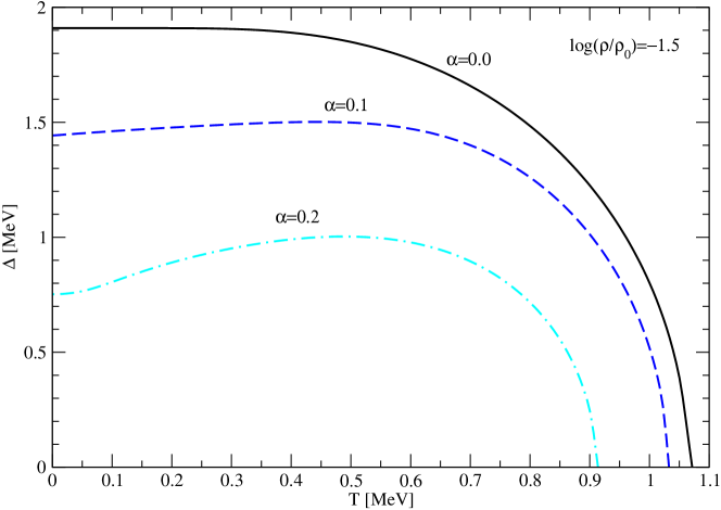
Figure 3.2: The gap as a function of the temperature at constant density $\log(\rho/\rho_{0})=-1.5$ for several polarizations. This figure is analog to Fig. 1.7.

In Figs. 3.2 and 3.3 we present the gap at fixed density $\log(\rho/\rho_{0})=-1.5$ (these figures are analog to Figs. 1.7 and 1.8). In Fig. 3.2 the gap is shown as a function of the temperature for various values of the polarization. For zero polarization, i.e., in the case of symmetrical BCS state, the value of the gap is largest because of the perfect overlap of Fermi surfaces of spin-up and down particles. The temperature dependence of the gap corresponds to the standard BCS behavior. Increasing the polarization has two effects: first, due to the separation of the Fermi surfaces the gap decreases and so does $T_{C}$. Second, it shifts the maximum of the gap from $T=0$ to nonvanishing temperatures. This shift, for large enough polarizations can lead to the appearance of a lower critical temperature (see subsection 1.3.2 for a discussion of this effect).

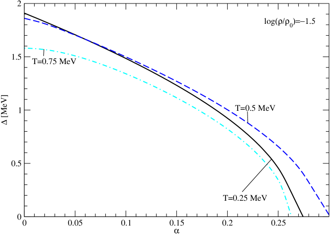
Figure 3.3: The gap as a function of the polarization at constant density $\log(\rho/\rho_{0})=-1.5$ for several temperatures. This figure is analog to Fig. 1.8.

In Fig. 3.3 the gap is shown as a function of the polarization for various temperatures. For $\alpha=0$ the temperature increase decreases the gap, as it should according to the BCS theory. The crossing of constant temperature curves at finite $\alpha$ reflects the fact that larger temperatures favor pairing in polarized systems, because they increase the overlap between the Fermi surfaces. Of course, this effect is counterbalanced by the destruction of the superfluid state by high enough temperatures. These arguments are reflected in the figure where at high enough polarizations the increase of temperature from $T=0.25$ MeV to $T=0.5$ MeV increases the gap, but the increase of the temperature from $T=0.5$ MeV to $T=0.75$ MeV again decreases the gap. See subsection 1.3.2 for a discussion of this behavior in the ${}^{3}S_{1}$-${}^{3}D_{1}$ condensate.

The kernel of the gap equation

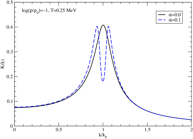
Figure 3.4: Dependence of the kernel $K(k)$ on momentum in units of Fermi momentum for fixed $\log(\rho/\rho_{0})=-1$, $T=0.25$ MeV, and various values of polarization indicated in the plot. This figure is analog to Fig. 1.15.

In Figs. 3.4-3.7 we present the kernel of the gap equation for various values of density, temperature and polarization in the BCS phase. Because we do not find a LOFF phase or a BEC, we do not discuss these regimes here. In the BCS case the formula for the kernel Eq. (1.61) simplifies to

$$K(k) = \sum_{r}\frac{P_{r}}{2\sqrt{E_{S}^{2}(k)+\Delta^{2}(k)}}\,,$$ (3.26)

with $P_{r}^{a}\rightarrow P_{r}$ for BCS pairing with ${\bm{Q}}=0$ (i.e., $E_{A}=0$). Figs. 3.4-3.6 show the kernel at $T=0.25$ MeV for various values of the polarization, the density being fixed for each figure. As expected in the case of $\alpha=0$ we find a single peak at the Fermi level. This peak separates into two for nonvanishing polarizations, which reflects the fact that there are now two Fermi surfaces for spin-up and spin-down particles. A further feature seen in Figs. 3.4-3.6 is that at high densities the peak of the kernel for $\alpha=0$ is located at $k=k_{F}$ exactly, whereas for low densities this peak is shifted to momenta below the corresponding $k_{F}$. In addition at lower densities the polarization induced two-peak structure is smeared, which is understood as due to the weakening of the degeneracy of the system.

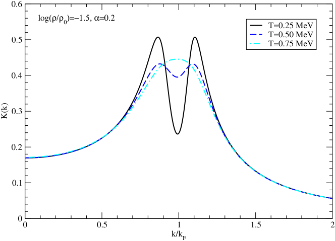
Figure 3.7: Dependence of the kernel $K(k)$ on momentum in units of Fermi momentum for fixed $\log(\rho/\rho_{0})=-1$, $\alpha=0.2$, and various temperatures indicated in the plot. This figure is analog to Fig. 1.14.

In Fig. 3.7 we present the kernel for constant density and polarization for different temperatures. We clearly see a temperature induced smearing of the polarization induced two peak structure resulting, which eventually results in a one peak structure at high temperatures. Further details to the behavior of the kernel under asymmetrical conditions can be found in subsection 1.3.5.

The Cooper-pair wave function

Next we want to discuss the Cooper-pair wave function $\Psi(r)$ and the quantity $r^{2}|\Psi(r)|^{2}$, which is the second moment of the density distribution of Cooper-pairs. Having at our disposal the wave function we can also access the coherence length $\xi_{\mathrm{rms}}$ of the condensate numerically. This then will be compared with the analytical BCS expression for the coherence length $\xi_{a}$ and the interparticle distance $d$. The definitions of these quantities are analogous to those defined in Eqs. (1.62)-(1.67); nevertheless we list them for convenience. The wave function is given by

$$\Psi(r) = \frac{\sqrt{N}}{2\pi^{2}r}\int_{0}^{\infty}dp\,p\,[K(p,\Delta)-K(p,0)]\sin(pr)\,,$$ (3.27)

and obeys the normalisation

$$1 = N\int d^{3}r|\Psi(r)|^{2}\,.$$ (3.28)

The root-mean-square (rms) value for the coherence length is given by

$$\xi_{\rm rms} = \sqrt{\langle r^{2}\rangle}\,,$$ (3.29)

where

$$\langle r^{2}\rangle \equiv \int d^{3}r\,r^{2}|\Psi(r)|^{2}\,.$$ (3.30)

The analytical BCS for the coherence length is given by

$$\xi_{a} = \frac{\hbar^{2}k_{F}}{\pi m^{*}\Delta}\,,$$ (3.31)

where now $\Delta$ is the pairing gap in the ${}^{1}S_{0}$ channel and $m^{*}$ is the effective mass of neutrons. Finally the interparticle distance is simply related to the net density of the system

$$d = \left(\frac{3}{4\pi\rho}\right)^{1/3}\,.$$ (3.32)

Further discussion of these quantities can be found in subsection 1.3.6.

Table 3.1 displays the quantities defined above for fixed temperature $T=0.25$ MeV and vanishing polarization and for several values of the density, specifically $\log(\rho/\rho_{0})=-1.0$, $\log(\rho/\rho_{0})=-1.5$ and $\log(\rho/\rho_{0})=-2.0$. We list for each density $k_{F}$, $\Delta$, $m^{*}/m$, $\mu_{n}$, $d$, $\xi_{\mathrm{rms}}$ and $\xi_{a}$. It is seen that at high densities $\xi_{\mathrm{rms}}\approx\xi_{a}$, i.e., the BCS analytical expression provides a good approximation to the numerically computed coherence length. This is not the case in the low density limit and we should rely only on the numerical value $\xi_{\mathrm{rms}}$. The comparison of the numerically computed coherence length with the interparticle distance shows a clear signature of BCS-BEC crossover, because for $\log(\rho/\rho_{0})=-1$ we find $\xi_{\mathrm{rms}}/d\approx 2$, whereas for $\log(\rho/\rho_{0})=-2$ we find that $\xi_{\mathrm{rms}}/d\approx 0.45$. We will trace the signatures of BCS-BEC crossover in other variables for spin-polarized neutron matter below.

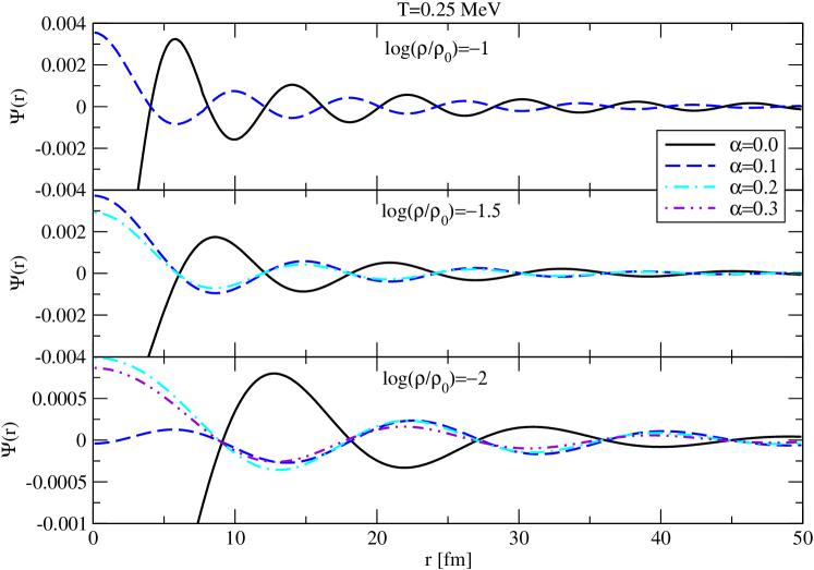
Figure 3.8: Dependence of $\Psi(r)$ on $r$ at fixed temperature $T=0.25$ MeV. Different panels show different densities and different colors show different values of the polarization as indicated in the plot. This figure is analog to Fig. 1.18.

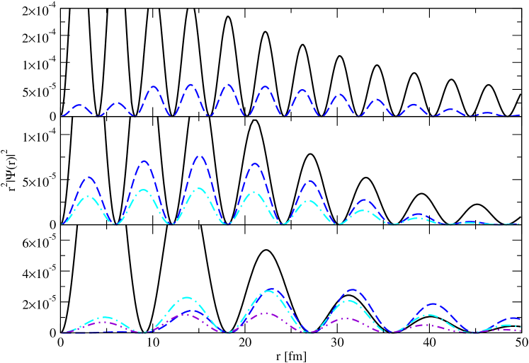
Figure 3.9: Dependence of $r^{2}|\Psi(r)|^{2}$ on $r$. The color code, the arrangement of the figures and the values for density, temperature and polarization are the same as in Fig. 3.8. This figure is analog to Fig. 1.19.

In Fig. 3.8 we show the Cooper-pair wave function $\Psi(r)$ as a function of radial distance for various densities and polarization at fixed temperature. In all cases we find strongly oscillating wave functions. For nonvanishing polarization, the wave function experiences a sign change (or, in other words, the oscillations are in counter-phase to the unpolarized case). An increasing polarization decreases the amplitude $\Psi(r)$, which is consistent with the fact that the pairing gap is reduced. Furthermore, the oscillation periods are given roughly by $2\pi/k_{F}$, therefore decreasing the densities and $k_{F}$ leads to the increase of the period of the oscillations. The degree of polarization does not effect the period, which is given by $k_{F}$. In Fig. 3.9 we show $r^{2}|\Psi(r)|^{2}$ as a function of radial distance under conditions fully analogous to Fig. 3.8. The oscillatory behavior discussed for the previous figure is reflected quite naturally in this quantity as well. A feature that is better visible here is that for the lowest density the maxima of the function for different polarizations are shifted with respect to each other; also the overall maximum reached for each polarization is not at the same value of $r$. We conclude that general features of the wave functions of ${}^{1}S_{0}$ pairing neutron matter discussed in this subsubsection are the same as those of ${}^{3}S_{1}$-${}^{3}D_{1}$ pairing nuclear matter, described in detail in subsection 1.3.6.

Occupation numbers

In this subsubsection we describe the occupation numbers of spin-up and spin-down neutrons in spin-polarized pure neutron matter. The occupation numbers are given by the integrand of Eq. (3.20). It simplifies in ${}^{1}S_{0}$ paired pure neutron matter in the BCS phase to the following

$$n_{\uparrow/\downarrow}(k) = \frac{1}{2}\left(1+\frac{E_{S}}{\sqrt{E_{S}^{2}+\Delta^{2}}}\right)f(E_{\mp})$$ (3.33)

$$+\frac{1}{2}\left(1-\frac{E_{S}}{\sqrt{E_{S}^{2}+\Delta^{2}}}\right)[1-f(E_{\pm})]\,,$$

with $E_{r}^{a}\rightarrow E_{r}$ for BCS pairing with ${\bm{Q}}=0$ (i.e., $E_{A}=0$). We note in passing that because of different degeneracy factor in neutron matter (no summation over spin) the maximum of functions $n_{\uparrow/\downarrow}(k)$ is $1$, instead of $2$ as in nuclear matter.

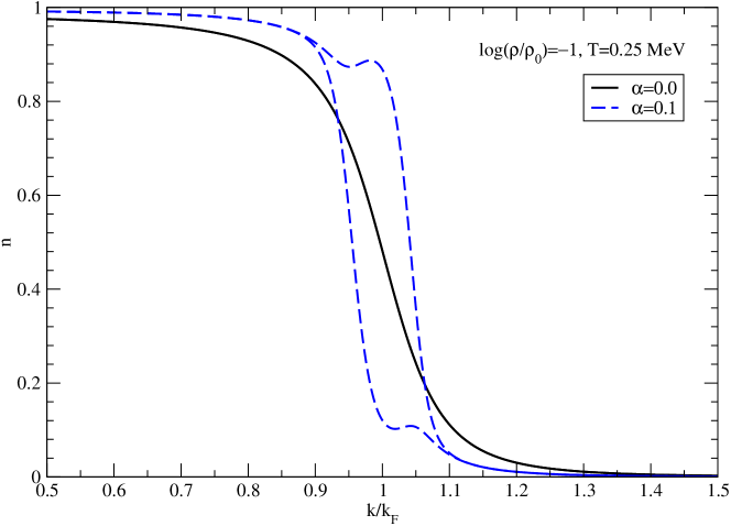
Figure 3.10: Dependence of the spin-up and spin-down neutron occupation numbers on momentum $k$ (in units of Fermi momentum) for fixed $\log(\rho/\rho_{0})=-1$, $T=0.25$ MeV, and various values of polarization indicated in the plot. This figure is analog to Fig. 1.24.

In Figs. 3.10-3.12 we display the occupation numbers of spin-up and down neutrons at fixed temperature $T=0.25$ MeV, fixed densities $\log(\rho/\rho_{0})$ $=-1$, $-1.5$ and $-2$, respectively. The polarizations are shown in the figures. In the case of vanishing polarization (solid lines) the Fermi step-function-like occupation in the high-density limit changes its slope into a “flatter” distribution at lower densities; this corresponds to a more diffuse Fermi surface at low densities. At finite polarizations the occupation numbers of spin-up and down particles split in the region around $k_{F}$. In fact, the locations of the drop in the occupations of these populations agree well with their corresponding Fermi wave-vectors. At high density the polarization induced splitting results in a “breach” for large polarizations with $n_{n\uparrow}=1$ and $n_{n\downarrow}=0$ around $k_{F}$. The breach remains intact at lower densities, but the slope of the corresponding occupation numbers changes as already observed for the case of unpolarized matter.

In 3.13 we show the occupation numbers of spin-up and spin-down neutrons at fixed density $\log(\rho/\rho_{0})=-1.5$ and fixed polarization $\alpha=0.2$ for different temperatures. The effect of temperature is to induce smearing of the occupation numbers with increasing temperature. More details can be found in subsection 1.3.3, where we discuss the temperature dependence of occupation numbers for ${}^{3}S_{1}$-${}^{3}D_{1}$ condensate and in subsection 1.3.7 where we give a general analysis of the occupation numbers.

Quasiparticle spectra

As a final intrinsic quantity of interest we consider the dispersion relations for quasiparticle excitations about the ${}^{1}S_{0}$ condensate. Because we do not find LOFF phase the quasiparticle branches $E_{\pm}^{-}=E_{\pm}^{+}$ are degenerated and we can drop the superscript altogether. Thus the quasiparticle spectrum is given by

$$E_{\pm}(k) = \sqrt{\left(\frac{k^{2}}{2m^{*}}-\bar{\mu}\right)^{2}+\Delta^{2}}\pm\delta\mu\,.$$ (3.34)

These dispersion relations are shown in Fig. 3.14 for various values of density and polarization for fixed temperature $T=0.25$ MeV. In each case the spectrum has a minimum at $k_{F}$. At finite polarization there is a splitting of spectra of spin-up and spin-down neutrons. Furthermore, for low densities the spectrum of minority (spin-down neutrons) crosses zero, which means that their spectrum is gapless. The overall behavior of the dispersion relations are analogous to that of the ${}^{3}S_{1}$-${}^{3}D_{1}$ condensate which we discussed in subsection 1.3.8.

3.3.3 Magnetic field strength

As mentioned earlier, the spin-polarization in pure neutron matter can be induced by a magnetic field. In this subsection we want to discuss the strength of the magnetic field needed to create a certain polarization and compare the corresponding energy $\varepsilon_{B}$ given by Eq. (3.25) with the temperature. We note however that the magnetic field is linearly related to the shift in the chemical potentials $\delta\mu$ and in essence our study is equivalent to the study of chemical potentials shift for given spin-polarization.

In Fig. 3.15 we display the magnetic field as a function of density at constant polarization and temperature. It is seen that to obtain a given spin-polarization stronger magnetic fields are needed for higher densities. That is, the dense matter is harder to polarize than the low density matter. This trend is reversed at and above approximately a tenth of the saturation density. The physical content of this observation is difficult to access because the chemical potential shift is non-trivially related to the polarization and the pairing gap. It is further seen from Fig. 3.15 that finite temperature matter is more easily polarizable at low densities, but this trend may reverse again at high densities. In Fig. 3.16 we fixed the temperature in each panel and present different polarizations with different colors. We then learn that a strong magnetic field is needed to achieve a large polarization in the low-density matter. This trend may again reverse in the high-density matter.

It is physically interesting to consider the ratio of the magnetic energy to the temperature in the parameter range discussed above, i.e., we are interested in

$$\frac{\varepsilon_{B}}{T}\approx-\frac{g_{n}}{2}\frac{e\hbar}{2mc}\frac{B}{T}.$$ (3.35)

This ratio shown in Figs. 3.17 and 3.18, where the arrangement of the figures and the color code are analogous to Fig. 3.15 and Fig. 3.16, respectively. We see that almost in the complete range of the parameter space $\varepsilon_{B}/T>1$; exceptions are the extreme low density limits in various plots.

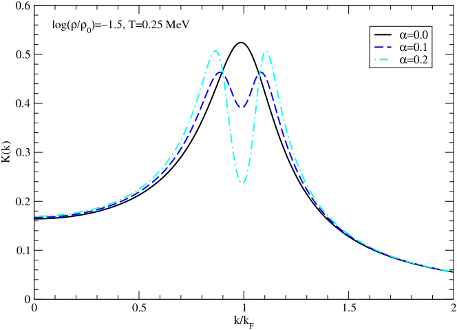
Figure 3.5: Same as Fig. 3.4 but for $\log(\rho/\rho_{0})=-1.5$ and three values for the polarization.

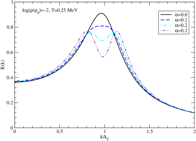
Figure 3.6: Same as Fig. 3.4 but for $\log(\rho/\rho_{0})=-2$ and more values for the polarization.

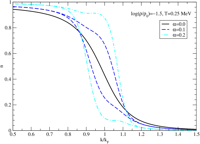
Figure 3.11: Same as Fig. 3.10 but for $\log(\rho/\rho_{0})=-1.5$ and more values for the polarization.

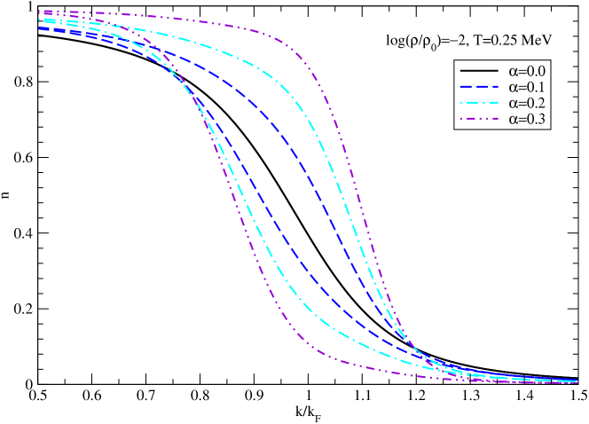
Figure 3.12: Same as Fig. 3.10 but for $\log(\rho/\rho_{0})=-2$ and more values for the polarization.

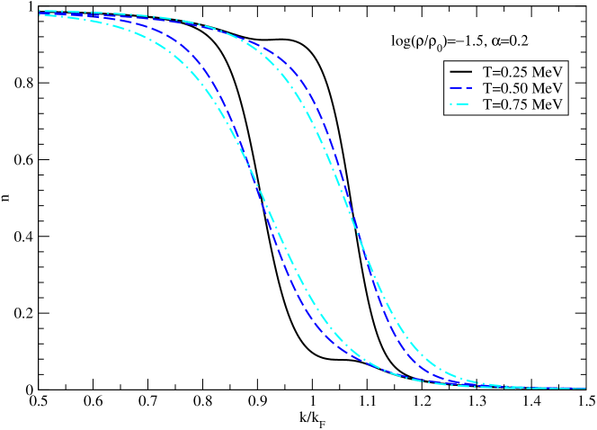
Figure 3.13: Dependence of the spin-up and spin-down neutron occupation numbers on momentum $k$ (in units of Fermi momentum) for fixed $\log(\rho/\rho_{0})=-1.5$, $\alpha=0.2$, and various temperatures indicated in the plot. This figure is analog to Fig. 1.9.

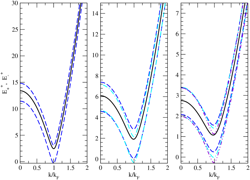
Figure 3.14: Dispersion relations for quasiparticle spectra in the case of the BCS condensate, as functions of momentum in units of Fermi momentum. For each polarization, the upper branch corresponds to $E^{+}_{+}$, and the lower to the $E^{+}_{-}$ solution. The color code, the arrangement of the figures and the values for density, temperature and polarization are the same as in Fig. 3.8. This figure is analog to Fig. 1.26.

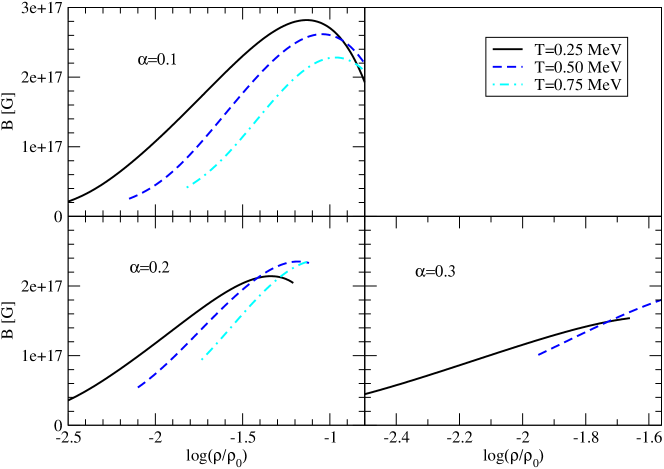
Figure 3.15: The needed magnetic field to create a certain spin-polarization as a function of the density. In each panel a certain polarization is fixed. Different temperatures are presented with different colors.

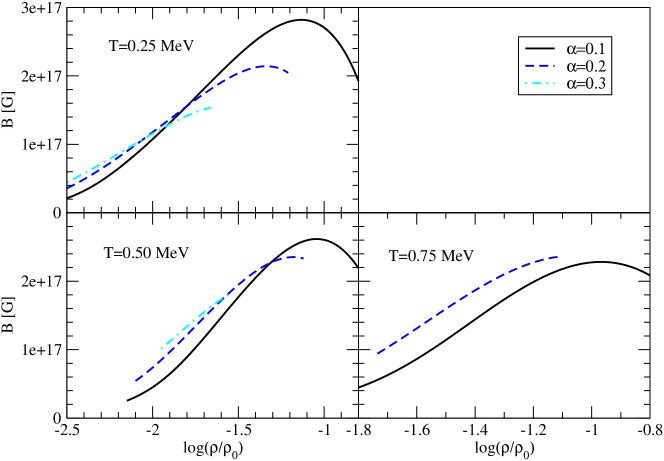
Figure 3.16: The needed magnetic field to create a certain spin-polarization as a function of the density. In each panel a certain temperature is fixed. Different values of polarization are presented with different colors.

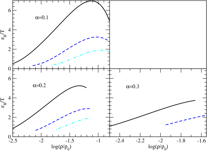
Figure 3.17: The magnetic energy divided by the temperature as a function of the density for different temperatures and values of polarization. The color code is the same as in Fig. 3.15.

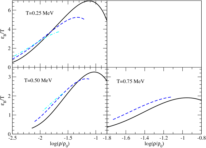
Figure 3.18: The magnetic energy divided by the temperature as a function of the density for different temperatures and values of polarization. The color code is the same as in Fig. 3.16.

3.4 Conclusion

The phase diagram of low-density spin-polarized neutron matter studied in this chapter has a simpler phase structure compared to the phase diagram of low-density isospin asymmetric nuclear matter studied in chapter 1. Because two neutrons can not form bound pairs, there exists no a priori BEC of neutron-neutron pairs. Moreover, there exists no LOFF phase, because the pairing gap is much too low compared to the chemical potential. Since the phase diagram consists of only BCS and unpaired phase, we have two critical temperatures at non-vanishing polarization.

Our analysis of this chapter can be summarized as follows:

• At low density, spin-polarization does not affect the pairing significantly. For high densities and high polarizations, the pairing gap and hence $T_{C}$ are significantly suppressed. At finite polarization and low temperatures we find a lower critical temperature due to the combination of the polarization induced separation and the temperature induced smearing of the Fermi edges.

• We studied some intrinsic features of spin-polarized neutron condensate, specifically, the gap, the kernel of the gap equation, the condensate wave functions, the occupation numbers and the quasiparticle spectrum. The similarities and differences to the low-density isospin asymmetric nuclear matter studied in chapter 1 have been highlighted. In the following we list the main features only.

• The gap has non-trivial dependence on the polarization and temperature. At finite polarizations the gap may be increased by increasing the temperature because of the restoration of the coherence among the spin-up and down population by the temperature.

• The kernel of the gap equation has a double peak structure compared to the non-polarized case. This structure is most pronounced in the high-density and low-temperature limit. Decreasing the density (or increasing the temperature) smears out this structure.

• The Cooper-pair wave functions have an oscillating behavior. At finite polarization the oscillations are in counter-phase to those in the unpolarized case. The period of the oscillations is defined by the wave vector as $2\pi/k_{F}$ and is not affected by the polarization.

• The occupation numbers show a separation of the majority and minority components by a “breach” around the Fermi momentum. This is most pronounced in the high-density and low-temperature limit, in which case the spin-down (minority) components is almost extinct. For high temperatures or low densities, this “breach” is smeared out.

• The study of dispersion relations shows that they have a standard BCS form in the unpolarized case and they become split into two branches at finite polarization which retains the general BCS shape. The minima of these spectra are at $k=k_{F}$, as it should. At larger polarizations the energy spectrum of the spin-down particles crosses the zero-energy level, which is a signature of gapless superconductivity. In other words, the Fermi surface of spin-down particles then features locations where modes can be excited without any energy cost.

• Finally, we studied the influence of the magnetic field on the spin-polarization. At low densities a relatively weak magnetic field is needed to generate a certain polarization. The magnetic field needed to generate a certain polarization in general increases with decreasing temperature and with increasing polarization. The energy of the magnetic field is in general higher than the temperature, except for low densities and high temperatures.

Appendix A Matsubara summations

First we rewrite the equation for $F_{np}^{\pm}$:

$$F_{np}^{\pm} = \frac{-i\Delta}{(ik_{\nu}-E^{+}_{\pm})(ik_{\nu}+E^{-}_{\mp})}$$ (A.1a)

$$\Rightarrow F_{np}^{\pm} = \frac{-i\Delta}{E^{+}_{\pm}+E^{-}_{\mp}}\cdot\left(\frac{1}{ik_{\nu}-E^{+}_{\pm}}-\frac{1}{ik_{\nu}+E^{-}_{\mp}}\right)$$ (A.1b)

$$\Rightarrow F_{np}^{\pm} = \frac{-i\Delta}{2\sqrt{E_{S}^{2}+\Delta^{2}}}\cdot\left(\frac{1}{ik_{\nu}-E^{+}_{\pm}}-\frac{1}{ik_{\nu}+E^{-}_{\mp}}\right)\,.$$ (A.1c)

For the Matsubara summation we first solve

$$S(\pm E) = \frac{1}{\beta}\sum_{\nu}\frac{1}{ik_{\nu}\pm E}=\frac{1}{\beta}\sum_{\nu}g(ik_{\nu})\,,$$ (A.2a)

$$I(\pm E) = \underset{R\rightarrow\infty}{\lim}\int\frac{dz}{2\pi i}g(z)f(z)=\sum_{i}\mathrm{Res}(z_{i})\,,$$ (A.2b)

with $z_{i}$ being the poles of $g(z)f(z)$ and $f(z)$ being the Fermi function.

$$f(z) = \frac{1}{e^{\beta z}+1}\Rightarrow z_{n}=\frac{(2n+1)\pi i}{\beta}$$ (A.3a)

$$\Rightarrow R_{n} = \underset{z\rightarrow(2n+1)\pi i/\beta}{\lim}\,\frac{z-(2n+1)\pi i/\beta}{e^{\beta z}+1}g(z)$$ (A.3b)

$$= \underset{z\rightarrow(2n+1)\pi i/\beta}{\lim}\,\frac{z-(2n+1)\pi i/\beta}{-1+\beta z+(2n+1)\pi i+1}g(z)$$

$$= \underset{z\rightarrow(2n+1)\pi i/\beta}{\lim}\,\frac{z-(2n+1)\pi i/\beta}{\beta z+(2n+1)\pi i}g(z_{n})$$

$$= -\frac{1}{\beta}g(z_{n})\,.$$

The next residuum we obtain at the pole of $g(z)$

$$R_{1} = \underset{z\rightarrow\mp E}{\lim}\,\frac{z\pm E}{z\pm E}f(z)$$ (A.4a)

$$= f(\mp E)\,,\qquad\qquad\qquad f(-E)=1-f(E)\,.$$ (A.4b)

Thus all together we obtain:

$$I(\pm E) = -\frac{1}{\beta}\sum_{\nu}g(ik_{\nu})+f(\mp E)$$ (A.5a)

$$\Rightarrow\frac{1}{\beta}\sum_{\nu}\frac{1}{ik_{\nu}\pm E} = f(\mp E)$$ (A.5b)

$$\Rightarrow\frac{1}{\beta}\sum_{\nu}F_{np}^{\pm} = \frac{-i\Delta}{2\sqrt{E_{S}^{2}+\Delta^{2}}}$$ (A.5c)

$$\cdot\frac{1}{\beta}\sum_{\nu}\left(\frac{1}{ik_{\nu}-E^{+}_{\pm}}-\frac{1}{ik_{\nu}+E^{-}_{\mp}}\right)$$

$$= \frac{-i\Delta}{2\sqrt{E_{S}^{2}+\Delta^{2}}}\left(f(E^{+}_{\pm})-f(-E^{-}_{\mp})\right)$$ (A.5d)

$$= \frac{i\Delta}{2\sqrt{E_{S}^{2}+\Delta^{2}}}\left(1-f(E^{+}_{\pm})-f(E^{-}_{\mp})\right)\,.$$ (A.5e)

Analogue we obtain:

$$\frac{1}{\beta}\sum_{\nu}F_{pn}^{\pm} = \frac{-i\Delta}{2\sqrt{E_{S}^{2}+\Delta^{2}}}\left(1-f(E^{+}_{\mp})-f(E^{-}_{\pm})\right)\,.$$ (A.6)

Next we need the Matsubara summation of $G$:

$$G_{n/p}^{\pm} = \frac{ik_{\nu}\pm\epsilon_{p/n}^{\mp}}{(ik_{\nu}-E^{+}_{\mp/\pm})(ik_{\nu}+E^{-}_{\pm/\mp})}\,.$$ (A.7)

For this purpose we introduce the following

$$S(\pm\epsilon) = \frac{1}{\beta}\sum_{\nu}\frac{ik_{\nu}\pm\epsilon}{(ik_{\nu}-E^{+})(ik_{\nu}+E^{-})}=\frac{1}{\beta}\sum_{\nu}g(ik_{\nu})\,,$$ (A.8a)

$$I(\pm\epsilon) = \underset{R\rightarrow\infty}{\lim}\int\frac{dz}{2\pi i}g(z)f(z)=\sum_{i}\mathrm{Res}(z_{i})\,,$$ (A.8b)

and obtain:

$$z_{n}= (2n+1)\pi i/\beta R_{n}= -\frac{1}{\beta}g(z_{n})\,,$$ (A.9a)

$$z_{1}= E^{+} R_{1}= \frac{E^{+}\pm\epsilon}{E^{+}+E^{-}}f(E^{+})\,,$$ (A.9b)

$$z_{2}= -E^{-} R_{2}= \frac{E^{-}\mp\epsilon}{E^{+}+E^{-}}(1-f(E^{-}))\,,$$ (A.9c)

which can be solved to

$$\frac{1}{\beta}\sum_{\nu}\frac{ik_{\nu}\pm\epsilon}{(ik_{\nu}-E^{+})(ik_{\nu}+E^{-})}$$ (A.10)

$$= \frac{E^{+}\pm\epsilon}{2\sqrt{E_{S}^{2}+\Delta^{2}}}f(E^{+})+\frac{E^{-}\mp\epsilon}{2\sqrt{E_{S}^{2}+\Delta^{2}}}(1-f(E^{-}))\,.$$

Thus we obtain:

$$\frac{1}{\beta}\sum_{\nu}G_{n/p}^{\pm}=\frac{1}{\beta}\sum_{\nu}\frac{ik_{\nu}\pm\epsilon_{p/n}^{\mp}}{(ik_{\nu}-E^{+}_{\mp/\pm})(ik_{\nu}+E^{-}_{\pm/\mp})}$$ (A.11a)

$$= \frac{E^{+}_{\mp/\pm}\pm\epsilon_{p/n}^{\mp}}{2\sqrt{E_{S}^{2}+\Delta^{2}}}f(E^{+}_{\mp/\pm})+\frac{E^{-}_{\pm/\mp}\mp\epsilon_{p/n}^{\mp}}{2\sqrt{E_{S}^{2}+\Delta^{2}}}(1-f(E^{-}_{\pm/\mp}))$$ (A.11c)

$$= \frac{1}{2}\left(1\pm\frac{E_{S}}{\sqrt{E_{S}^{2}+\Delta^{2}}}\right)f(E^{+}_{\mp/\pm})$$

$$+\frac{1}{2}\left(1\mp\frac{E_{S}}{\sqrt{E_{S}^{2}+\Delta^{2}}}\right)(1-f(E^{-}_{\pm/\mp}))\,.$$

These summations will be needed for further calculations.

Appendix B Description of the TDHF Code

This appendix gives a brief overview of the code Sky3D adopted form Ref. [50]; there a more detailed discussion can be found.

B.1 Local densities and currents

The code calculates with a set of single-particle (s.p.) wave functions $\psi_{\alpha}$, with $\alpha\leq\Omega$, with $\Omega$ denoting the size of the active single particle (s.p.) space. For non-occupied states, $\psi_{\alpha}$ vanishes.

For the description of the Skyrme-energy-density functional only a few local densities and currents are needed. The time-even fields are given by

$$\rho_{q}(\bm{r})= \sum_{\alpha\in q}\sum_{s}\left|\psi_{\alpha}(\bm{r},s)\right|^{2} \text{density}\,,$$ (B.1a)

$${\bm{J}}_{q}(\bm{r})= -\mathrm{i}\sum_{\alpha\in q}\sum_{ss^{\prime}}\psi^{*}_{\alpha}(\bm{r},s)\nabla\times{\bm{\sigma}}_{ss^{\prime}}\psi_{a}(\bm{r},s^{\prime}) \text{spin-orbit density}\,,$$ (B.1b)

$$\tau_{q}(\bm{r})= \sum_{\alpha\in q}\sum_{s}\left|\nabla\psi_{\alpha}(\bm{r},s)\right|^{2} \text{kinetic density}\,,$$ (B.1c)

and for the time-odd fields one has

$${\bm{s}}_{q}(\bm{r})= \sum_{\alpha\in q}\sum_{ss^{\prime}}\psi^{*}_{\alpha}(\bm{r},s){\bm{\sigma}}_{ss^{\prime}}\psi_{a}(\bm{r},s^{\prime}) \text{spin density}\,,$$ (B.1d)

$${\bm{j}}_{q}(\bm{r})= \Im\left\{\sum_{\alpha\in q}\sum_{s}\psi^{*}_{\alpha}(\bm{r},s)\nabla\psi_{\alpha}(\bm{r},s)\right\} \text{current density}\,,$$ (B.1e)

with $q$ labels the isospin with $q=p$ for protons and $q=n$ for neutrons. A local density/current without index $q$ is the total density/current; for example $\rho=\rho_{p}+\rho_{n}$. The variable $s$ represents the two spinor components of the wave functions. The terms are understood as functions of $\bm{r}$. In addition to these terms, the pairing density [50] and the time-odd kinetic spin-density can be defined; moreover it is possible to define the spin-orbit density as a tensor, see Ref. [49].

B.2 The energy-density functional

The terms of Eq. (2.1) using the force coefficients of appendix B.3 are given by

• $T$: the total kinetic energy given by

  $$T=\sum_{q}\frac{\hbar^{2}}{2m_{q}}\int d^{3}r\,\tau_{q}\,,$$ (B.2a)

  with $\tau_{q}$ being the kinetic density of Eq. B.1c.

• $E_{0}$: the $b_{0}$ and $b^{\prime}_{0}$-dependent part is given by

  $$E_{0}=\int d^{3}r\left(\frac{b_{0}}{2}\rho^{2}-\frac{b^{\prime}_{0}}{2}\sum_{q}\rho^{2}_{q}\right)\,.$$ (B.2b)

• $E_{1}$: kinetic terms which contain the coefficients $b_{1}$ and $b^{\prime}_{1}$:

  $$E_{1}=\int d^{3}r\left(b_{1}\left[\rho\tau-{\bm{j}}^{2}\right]-b^{\prime}_{1}\sum_{q}\left[\rho_{q}\tau_{q}-{\bm{j}}_{q}^{2}\right]\right)\,.$$ (B.2c)

• $E_{2}$: terms which contain the coefficients $b_{2}$ and $b^{\prime}_{2}$. They include the Laplacians of the densities

  $$E_{2} = \int d^{3}r\left(-\frac{b_{2}}{2}\rho\nabla\rho+\frac{b^{\prime}_{2}}{2}\sum_{q}\rho_{q}\nabla\rho_{q}\right)\,.$$ (B.2d)

• $E_{3}$: the many-body contribution

  $$E_{3}=\int d^{3}r\left(\frac{b_{3}}{3}\rho^{\alpha+2}-\frac{b^{\prime}_{3}}{3}\rho^{\alpha}\sum_{q}\rho_{q}^{2}\right)\,.$$ (B.2e)

• $E_{ls}$: the spin-orbit energy is given by

  $$E_{ls} = \int d^{3}r\left(-b_{4}\left[\rho\nabla\cdot{\bm{J}}+{\bm{s}}\cdot\left(\nabla\times{\bm{j}}\right)\right]\right.$$ (B.2f)

  $$\left.-b^{\prime}_{4}\sum_{q}\left[\rho_{q}\nabla\cdot{\bm{J}}_{q}+{\bm{s}}_{q}\cdot\left(\nabla\times{\bm{j}}_{q}\right)\right]\right)\,.$$

• $E_{C}$: the Coulomb energy. It consists of the Hartree term, which includes the standard expression of a charge distribution of the own field of the nucleus and the exchange term in the Slater approximation. It is given by:

  $$E_{C} = \frac{e^{2}}{2}\int d^{3}rd^{3}r^{\prime}\frac{\rho_{p}(\bm{r})\rho_{p}(\bm{r}^{\prime})}{\left|\bm{r}-\bm{r}^{\prime}\right|}$$ (B.2g)

  $$-\int d^{3}r\frac{3e^{2}}{4}\left(\frac{3}{\pi}\right)^{1/3}\rho_{p}^{4/3}\,,$$

  with $e^{2}=1.43989$ MeV$\cdot$fm being the elementary charge unit.

• $E_{\mathrm{corr}}$: this term is for all additional corrections beyond mean field. Most calculations consider at least the center-of-mass correction $E_{cm}$.

This set-up ignores tensor spin-orbit and spin-spin coupling, these may be important for magnetic excitations and odd nuclei. They could have a significant influence of the studies of chapter 2, because the magnetic field breaks the time-reversal invariance. However, these applications are not the main objective of the TDHF approach. A detailed description of all conceivable bilinear forms in the densities and currents – (B.1) and additional ones – up to second order derivatives and a discussion of the importance of the single terms can be found in Ref. [49]. Only time reversal invariant combinations are allowed. In particular time-odd currents and densities need to appear in bilinear form to render the functional time-reversal invariant [49]. Only the term $\propto\rho^{2}$ is of zeroth order derivative, all other terms are of second order. Taking all terms into account leads to a second term of zeroth order derivative, being proportional to ${\bm{s}}^{2}$. All coupling constants in Eqs. (B.2b) to (B.2f) might depend on the density $\rho$. This dependence is approximated by the terms proportional to $\rho^{\alpha}$ in Eq. (B.2e) [49].

The most general form of the energy-density functional contains 23 free parameters. Galilean invariance reduces the free parameters to 17. Further assumptions and introducing a Skyrme force from [76] reduces the number of independent parameters to 10 [49]. The Skyrme forces work best for closed shells. For even states it works better than for uneven states [76]. In chapter 2 we analyse the double magic [16]O core and the even [12]C and [20]Ne cores.

B.3 Force coefficients

In the formulations above the parameters $b_{0},\,b^{\prime}_{0},\,\dots\,b^{\prime}_{4}$ are used, which are related to the constants appearing in the Skyrme force, which is a density-dependent force with zero-range of interaction. These relations are given by

$$\begin{split}b_{0}&=t_{0}\left(1+\tfrac{1}{2}x_{0}\right)\,,\\ b^{\prime}_{0}&=t_{0}\left(\tfrac{1}{2}+x_{0}\right)\,,\\ b_{1}&=\tfrac{1}{4}\left[t_{1}\left(1+\tfrac{1}{2}x_{1}\right)+t_{2}\left(1+\tfrac{1}{2}x_{2}\right)\right]\,,\\ b^{\prime}_{1}&=\tfrac{1}{4}\left[t_{1}\left(\tfrac{1}{2}+x_{1}\right)-t_{2}\left(\tfrac{1}{2}+x_{2}\right)\right]\,,\\ b_{2}&=\tfrac{1}{8}\left[3t_{1}\left(1+\tfrac{1}{2}x_{1}\right)-t_{2}\left(1+\tfrac{1}{2}x_{2}\right)\right]\,,\\ b^{\prime}_{2}&=\tfrac{1}{8}\left[3t_{1}\left(\tfrac{1}{2}+x_{1}\right)+t_{2}\left(\tfrac{1}{2}+x_{2}\right)\right]\,,\\ b_{3}&=\tfrac{1}{4}t_{3}\left(1+\tfrac{1}{2}x_{3}\right)\,,\\ b^{\prime}_{3}&=\tfrac{1}{4}t_{3}\left(\tfrac{1}{2}+x_{3}\right)\,,\\ b_{4}&=\tfrac{1}{2}t_{4}\,.\\ \end{split}$$ (B.3)

The coefficient $b^{\prime}_{4}$ is usually fixed to $b^{\prime}_{4}=\frac{1}{2}t_{4}$ for most traditional Skyrme forces, but it can be handled separately as a free parameter. In addition to the $b$ and $b^{\prime}$ parameters, the power coefficient $\alpha$ is included, it is needed e.g. in Eq. (B.2e). For the input of the force one thus needs to specify the values of the $t_{i},\,x_{i}$ coefficients.

B.4 The single-particle Hamiltonian

The first term in Eq. (2.2) is the local part of the mean field. It acts on the wave functions like a local potential. Its definition is as follows

$$U_{q} = b_{0}\rho-b^{\prime}_{0}\rho_{q}+b_{1}\tau-b^{\prime}_{1}\tau_{q}-b_{2}\nabla\rho+b^{\prime}_{2}\nabla\rho_{q}$$ (B.4a)

$$+b_{3}\frac{\alpha+2}{3}\rho^{\alpha+1}-b^{\prime}_{3}\frac{2}{3}\rho^{\alpha}\rho_{q}-b^{\prime}_{3}\frac{\alpha}{3}\rho^{\alpha-1}\sum_{q^{\prime}}\rho^{2}_{q^{\prime}}$$

$$-b_{4}\nabla\cdot{\bm{J}}-b^{\prime}_{4}\nabla\cdot{\bm{J}}_{q}\,.$$

The second term in Eq. (2.2) referes to the kinetic energy of nucleons, where the “effective mass” is introduced by replacing the free-space factor $$\hbar^{2}/(2m)$$ by the isospin and space dependent factor

$$B_{q} = \frac{\hbar^{2}}{2m_{q}}+b_{1}\rho-b^{\prime}_{1}\rho_{q}\,.$$ (B.4b)

It is clear that this factor depends on a particular parameterization of the Skyrme force as well as on the isospin. The third term in Eq. (2.2) is the spin-orbit potential which is given by

$$\bm{W}_{q} = b_{4}\nabla\rho+b^{\prime}_{4}\nabla\rho_{q}\,.$$ (B.4c)

Eqs. (B.4a)-(B.4c) above are time-even contribution to the Hamiltonian operator $$\hat{h}_{q}$$. Dynamical effects may enter due to the fourth and fifth terms in Eq. (2.2) which are time-odd and involve contributions from current and spin-density,

$$\bm{A}_{q} = -2b_{1}{\bm{j}}+2b^{\prime}_{1}{\bm{j}}_{q}-b_{4}\nabla\times{\bm{s}}-b^{\prime}_{4}\nabla\times{\bm{s}}_{q}\,,$$ (B.4d)

$${\bm{S}}_{q} = -b_{4}\nabla\times{\bm{j}}-b^{\prime}_{4}\nabla\times{\bm{j}}_{q}\,.$$ (B.4e)

B.5 Static Hartree-Fock

The code Sky3D uses an iterative method for the solution of the problem at hand. The wave function in the step $n+1$ is related to the wave-function at step $n$ by the relation

$$\psi_{\alpha}^{(n+1)}=\mathcal{O}\left\{\psi_{\alpha}^{(n)}-\frac{\delta}{\hat{T}+E_{0}}\left(\hat{h}^{(n)}-\left<\psi_{\alpha}^{(n)}\middle|\hat{h}^{(n)}\middle|\psi_{\alpha}^{(n)}\right>\right)\psi_{\alpha}^{(n)}\right\}\,,$$ (B.5)

with $\hat{T}=\hat{p}^{2}/(2m)$ being the operator of the kinetic energy, $\mathcal{O}$ means orthonormalization of the whole set of new wave functions, the upper index $n$ is the iteration number. To accelerate the iteration a damping of the kinetic term is performed. This kinetic-energy damping is particularly suited if one employs the FFT (fast Fourier transformation) method. The damped gradient step has two numerical parameters: the step size $\delta$ and the damping regulator $E_{0}$. The latter should be chosen of order of the depth of the local potential $U_{q}$, hereby $E_{0}=100$ MeV is found to be a save choice, the step size should be in the range $\delta=0.1\dots 0.8$. Larger values lead to a faster iteration, but they are more likely to result in wrong values. The optimal value depends among other things on the choice of the Skyrme parametrization. The use of $m^{*}/m\approx 1$ allows larger values of $\delta$ and analogous lower values are needed for low $m^{*}/m$.

After performing one of these wave function iteration steps, the densities of Eqs. (B.1a) to (B.1e) are updated and new mean fields are computed according to Eq. (2.2). This provides the starting point for the next iteration. The iterations are continued until sufficient convergence is achieved. As convergence criterion the average energy variance or the fluctuation of single particle states is used:

$$\overline{\Delta\varepsilon} = \sqrt{\frac{\sum_{\alpha}\Delta\varepsilon_{\alpha}^{2}}{\sum_{\alpha}1}}\,,$$ (B.6a)

$$\Delta\varepsilon_{\alpha}^{2} = \left<\psi_{\alpha}\middle|\hat{h}^{2}\middle|\psi_{\alpha}\right>-\varepsilon_{\alpha}^{2}\,,$$ (B.6b)

$$\varepsilon_{\alpha} = \left<\psi_{\alpha}\middle|\hat{h}\middle|\psi_{\alpha}\right>\,,$$ (B.6c)

with the single particle energy $\varepsilon_{\alpha}$ being the expectation value of the Hamiltonian. It becomes the eigenvalue of Eq. (2.3) once the convergence is achieved, i.e., $\Delta\varepsilon_{\alpha}\approx 0$. When the total variance $\overline{\Delta\varepsilon}$ vanishes, a minimum energy of mean-field is reached. However, the minimum found with this method may be a metastable local minimum.

The initialization in the code Sky3D is realized by implementing the wave functions of a deformed harmonic oscillator. Hereby the states with lowest oscillator energy are implemented first. This initialization influences the initial state and the resulting final state, see Ref. [50] for further details.

B.6 Observables

The output of the code are the observables, which in the case of Hartree-Fock theory are the energy of the nucleus and the densities of nucleons. The density distribution can be described in terms of multipole moments. To treat the center of mass motion the Cartesian center-of-mass vector for neutrons and protons is introduced

$${\bm{R}}_{q}=\frac{\int d^{3}r\bm{r}\rho_{q}(\bm{r})}{A}\,,$$ (B.7a)

where $$A=\int d^{3}r\rho(\bm{r})$$ is the total mass number. Furthermore one can introduce the iso-scalar or total center-of-mass vector as

$${\bm{R}}_{T=0}=\frac{\int d^{3}r\bm{r}(\rho_{p}+\rho_{n})(\bm{r})}{A}\,,$$ (B.7b)

as well as an iso-vector center-of-mass vector

$${\bm{R}}_{T=1}=\frac{\int d^{3}r\bm{r}\left(\frac{N}{A}\rho_{p}-\frac{Z}{A}\rho_{n}\right)(\bm{r})}{A}\,.$$ (B.7c)

The same relations can be written for the corresponding quadrupole moments, for example,

$$\mathcal{Q}_{kl}^{q} = \int d^{3}r\left(3\left(r_{k}-R_{k}\right)\left(r_{l}-R_{l}\right)\right.$$ (B.7d)

$$\left.-\delta_{kl}\sum_{i}\left(r_{i}-R_{i}\right)^{2}\right)\rho^{q}\left(\bm{r}\right)\,,$$

and other defined in a simular way. The matrix $$\mathcal{Q}_{kl} Q_{xx} Q_{yy} Q_{zz} Q_{xx}+Q_{yy}+Q_{zz}=0 \mathcal{Q}_{kl}$$ is not invariant under rotations of the coordinate frame. The preferred coordinate system is the system of principle axes, where there are only three non-vanishing components , and with the trace . The general matrix can be diagonalized by appropriate rotations.

It is also useful to introduce the spherical moments for the quadrupole case

$$Q_{2m}^{q}=\int d^{3}rr^{2}Y_{2m}\rho^{q}\left(\bm{r}-{\bm{R}}\right)\,,$$ (B.7e)

with $r=\left|\bm{r}\right|$ being the absolute of $\bm{r}$ and $Y_{2m}$ being the spherical harmonics. The latter are often expressed as dimensionless quadrupole moments:

$$a_{m}=\frac{4\pi}{5}\frac{Q_{2m}}{AR^{2}}\,,$$ (B.7f)

with $R=r_{0}A^{1/3}$ being a fixed radius of the nucleus which depends only on the total mass number $A$. This expression again could be calculated for any type of moments, but in practice it is mainly used for isoscalar moments.

Having dimensionless moments is an advantage, because they are free of an overall scale which is removed by the division by the factor $AR^{2}$. This description allows a characterization of the shape of the nucleus. The general $a_{m}$ are not invariant under rotations of the coordinate frame. A unique characterization is obtained by a transformation into the system of principle-axes. Here we have the following conditions: $a_{\pm 1}=0$ and $a_{2}=a_{-2}$, thus there are two remaining shape parameters: $a_{0}$ and $a_{2}$. They can be re-expressed by the total deformation $\beta$ and the triaxiality $\gamma$, which are often called the Bohr-Mottelson parameters and are defined in the following way

$$\beta=\sqrt{a_{0}^{2}+2a_{2}^{2}}\,,\quad\gamma=\arctan\left(\frac{\sqrt{2}a_{2}}{a_{0}}\right)\,.$$ (B.7g)

The triaxiality $\gamma$ is handled like an angle. In general it can take values between $0\degree$ and $360\degree$. However the physical relevant region is from $0\degree$ to $60\degree$. The other sectors lead to equivalent configurations [73].

The r.m.s. radii of neutrons and protons are defined as follows

$$r_{\mathrm{rms}}^{q}=\sqrt{\frac{\int d^{3}r\left(\bm{r}-{\bm{R}}\right)^{2}\rho^{q}\left(\bm{r}\right)}{\int d^{3}r\rho^{q}\left(\bm{r}\right)}}\,.$$ (B.7h)

Similarly one can define the total r.m.s. radius of a nucleus by replacing $\rho^{q}$ by the total density $\rho$.

The total energy $E_{\mathrm{tot}}$ can be computed in two alternative ways. One is to use the formula (2.1). The alternative starts with the equation for the energy [73]

$$E_{\mathrm{tot,\,HF}}=\frac{1}{2}\sum_{\alpha}\left(t_{\alpha}+\varepsilon_{\alpha}\right)\,,$$ (B.8)

with $t_{\alpha}=\left<\psi_{\alpha}\middle|\hat{T}\middle|\psi_{\alpha}\right>$ being the s.p. kinetic energy and the quantity $\varepsilon_{\alpha}$ is defined as

$$\varepsilon_{\alpha} = t_{\alpha}+u_{\alpha}\,,\quad u_{\alpha}=\sum_{\beta}\left[v_{\alpha\beta\alpha\beta}-v_{\alpha\beta\beta\alpha}\right]=\varepsilon_{\alpha}-t_{\alpha}\,,$$

with $u_{\alpha}$ being the s.p. mean-field potential energy and $v$ the two body interaction; leading to:

$$E_{\mathrm{tot,\,HF}}=\sum_{\alpha}t_{\alpha}+\frac{1}{2}\sum_{\alpha\beta}\left[v_{\alpha\beta\alpha\beta}-v_{\alpha\beta\beta\alpha}\right]\,.$$

In the case of Skyrme forces, additional rearrangement energies should be added [50]. In the code Sky3D the total energy is computed in both ways: from the straightforward Skyrme energy of Eq. (2.1) and using a modified version of Eq. B.8.

References

- [1] D. E. Sheehy and L. Radzihovsky. BEC BCS crossover, phase transitions and phase separation in polarized resonantly-paired superfluids. Annals of Physics, 322:1790–1924, August 2007.
- [2] S. Giorgini, L. P. Pitaevskii, and S. Stringari. Theory of ultracold atomic Fermi gases. Reviews of Modern Physics, 80:1215–1274, October 2008.
- [3] A. Sedrakian. BCS-BEC crossover in spatially modulated fermionic condensates. Journal of Physics Conference Series, 321(1):012028, September 2011.
- [4] A. Sedrakian and D. H. Rischke. Phase diagram of chiral quark matter: From weakly to strongly coupled Fulde-Ferrell phase. Phys. Rev. D, 80(7):074022, October 2009.
- [5] C.-F. Mu, L.-Y. He, and Y.-X. Liu. Evaluating the phase diagram at finite isospin and baryon chemical potentials in the Nambu-Jona-Lasinio model. Phys. Rev. D, 82(5):056006, September 2010.
- [6] J. Moreira, B. Hiller, W. Broniowski, A. A. Osipov, and A. H. Blin. Nonuniform phases in a three-flavor Nambu-Jona-Lasinio model. Phys. Rev. D, 89(3):036009, February 2014.
- [7] I. E. Frolov, V. C. Zhukovsky, and K. G. Klimenko. Chiral density waves in quark matter within the Nambu-Jona-Lasinio model in an external magnetic field. Phys. Rev. D, 82(7):076002, October 2010.
- [8] T. Kojo, Y. Hidaka, K. Fukushima, L. D. McLerran, and R. D. Pisarski. Interweaving chiral spirals. Nuclear Physics A, 875:94–138, February 2012.
- [9] M. Baldo, U. Lombardo, and P. Schuck. Deuteron formation in expanding nuclear matter from a strong coupling BCS approach. Phys. Rev. C, 52:975–985, August 1995.
- [10] B. Cederwall, F. G. Moradi, T. Bäck, A. Johnson, J. Blomqvist, E. Clément, G. de France, R. Wadsworth, K. Andgren, K. Lagergren, A. Dijon, G. Jaworski, R. Liotta, C. Qi, B. M. Nyakó, J. Nyberg, M. Palacz, H. Al-Azri, A. Algora, G. de Angelis, A. Ataç, S. Bhattacharyya, T. Brock, J. R. Brown, P. Davies, A. di Nitto, Z. Dombrádi, A. Gadea, J. Gál, B. Hadinia, F. Johnston-Theasby, P. Joshi, K. Juhász, R. Julin, A. Jungclaus, G. Kalinka, S. O. Kara, A. Khaplanov, J. Kownacki, G. La Rana, S. M. Lenzi, J. Molnár, R. Moro, D. R. Napoli, B. S. N. Singh, A. Persson, F. Recchia, M. Sandzelius, J.-N. Scheurer, G. Sletten, D. Sohler, P.-A. Söderström, M. J. Taylor, J. Timár, J. J. Valiente-Dobón, E. Vardaci, and S. Williams. Evidence for a spin-aligned neutron-proton paired phase from the level structure of 92Pd. Nature, 469:68–71, January 2011.
- [11] S. Mao, X. Huang, and P. Zhuang. BCS-BEC crossover and thermodynamics in asymmetric nuclear matter with pairings in isospin I=0 and I=1 channels. Phys. Rev. C, 79(3):034304, March 2009.
- [12] A. Pastore, J. Margueron, P. Schuck, and X. Viñas. Pairing in exotic neutron-rich nuclei near the drip line and in the crust of neutron stars. Phys. Rev. C, 88(3):034314, September 2013.
- [13] Masayuki Matsuo. Spatial structure of neutron cooper pair in low density uniform matter. Phys. Rev. C, 73:044309, Apr 2006.
- [14] J. Margueron, H. Sagawa, and K. Hagino. BCS-BEC crossover of neutron pairs in symmetric and asymmetric nuclear matter. Phys. Rev. C, 76(6):064316, December 2007.
- [15] A. A. Isayev. Correlation functions for a di-neutron condensate in asymmetric nuclear matter. Phys. Rev. C, 78(1):014306, July 2008.
- [16] S. Gandolfi, A. Y. Illarionov, F. Pederiva, K. E. Schmidt, and S. Fantoni. Equation of state of low-density neutron matter, and the 1S0 pairing gap. Phys. Rev. C, 80(4):045802, October 2009.
- [17] A. Sedrakian and J. W. Clark. Nuclear Superconductivity in Compact Stars: BCS Theory and Beyond, page 135. World Scientific Publishing Co, 2006.
- [18] M. Stein, X.-G. Huang, A. Sedrakian, and J. W. Clark. Phase diagram of dilute nuclear matter: Unconventional pairing and the BCS-BEC crossover. Phys. Rev. C, 86(6):062801, December 2012.
- [19] M. Stein, A. Sedrakian, X.-G. Huang, and J. W. Clark. BCS-BEC crossovers and unconventional phases in dilute nuclear matter. Phys. Rev. C, 90(6):065804, December 2014.
- [20] J. Haidenbauer and W. Plessas. Separable representation of the Paris nucleon-nucleon potential. Phys. Rev. C, 30:1822–1839, December 1984.
- [21] R. K. Su, S. D. Yang, and T. T. S. Kuo. Liquid-gas and superconducting phase transitions of nuclear matter calculated with real time Green’s function methods and Skyrme interactions. Phys. Rev. C, 35:1539–1550, April 1987.
- [22] A. Sedrakian and U. Lombardo. Thermodynamics of a n-p Condensate in Asymmetric Nuclear Matter. Physical Review Letters, 84:602, January 2000.
- [23] P. Nozières and S. Schmitt-Rink. Bose condensation in an attractive fermion gas: From weak to strong coupling superconductivity. Journal of Low Temperature Physics, 59:195–211, May 1985.
- [24] D. M. Eagles. Possible Pairing without Superconductivity at Low Carrier Concentrations in Bulk and Thin-Film Superconducting Semiconductors. Physical Review, 186:456–463, October 1969.
- [25] T. Alm, B. L. Friman, G. Röpke, and H. Schulz. Pairing instability in hot asymmetric nuclear matter. Nuclear Physics A, 551:45–53, January 1993.
- [26] H. Stein, A. Schnell, T. Alm, and G. Röpk. Correlations and pairing in nuclear matter within the Nozières-Schmitt-Rink approach. Zeitschrift fur Physik A Hadrons and Nuclei, 351:295–299, September 1995.
- [27] U. Lombardo and P. Schuck. Size shrinking of deuterons in very dilute superfluid nuclear matter. Phys. Rev. C, 63(3):038201, March 2001.
- [28] A. Sedrakian and J. W. Clark. Pair condensation and bound states in fermionic systems. Phys. Rev. C, 73(3):035803, March 2006.
- [29] X.-G. Huang. BCS-BEC crossover in symmetric nuclear matter at finite temperature: Pairing fluctuation and pseudogap. Phys. Rev. C, 81(3):034007, March 2010.
- [30] M. Jin, M. Urban, and P. Schuck. BEC-BCS crossover and the liquid-gas phase transition in hot and dense nuclear matter. Phys. Rev. C, 82(2):024911, August 2010.
- [31] A. Sedrakian. Selected problems in astrophysics of compact objects. Journal of Physics Conference Series, 413(1):012024, February 2013.
- [32] M. Stein, A. Sedrakian, X.-G. Huang, J. W. Clark, and G. Röpke. Inhomogeneous condensates in dilute nuclear matter and BCS-BEC crossovers. Journal of Physics Conference Series, 496(1):012008, March 2014.
- [33] X.-l. Shang and W. Zuo. Angle-dependent gap state in asymmetric nuclear matter. Phys. Rev. C, 88(2):025806, August 2013.
- [34] X. Shang and W. Zuo. The FFLO state with angle dependent Gap in Asymmetric Nuclear Matter. ArXiv e-prints, August 2013.
- [35] B. Y. Sun and W. Pan. Dineutron correlations and BCS-BEC crossover in nuclear matter with the Gogny pairing force. Nuclear Physics A, 909:8–19, July 2013.
- [36] C. Regal. Experimental realization of BCS-BEC crossover physics with a Fermi gas of atoms. PhD thesis, University of Colorado at Boulder, 2006.
- [37] A. Sedrakian. Spatially inhomogeneous condensate in asymmetric nuclear matter. Phys. Rev. C, 63(2):025801, February 2001.
- [38] H. Müther and A. Sedrakian. Phases of asymmetric nuclear matter with broken space symmetries. Phys. Rev. C, 67(1):015802, January 2003.
- [39] A. I Larkin and Y. N. Ovchinnikov. Nonuniform state of superconductors. Zh. Eksp. Teor. Fiz., 47:762, 1965.
- [40] P. Fulde and R. A. Ferrell. Superconductivity in a Strong Spin-Exchange Field. Physical Review, 135:550–563, August 1964.
- [41] P. F. Bedaque, H. Caldas, and G. Rupak. Phase Separation in Asymmetrical Fermion Superfluids. Physical Review Letters, 91(24):247002, December 2003.
- [42] A. Broderick, M. Prakash, and J. M. Lattimer. The Equation of State of Neutron Star Matter in Strong Magnetic Fields. Astrophys. J., 537:351–367, July 2000.
- [43] M. Sinha, X.-G. Huang, and A. Sedrakian. Strange quark matter in strong magnetic fields within a confining model. Phys. Rev. D, 88(2):025008, July 2013.
- [44] M. Sinha, B. Mukhopadhyay, and A. Sedrakian. Hypernuclear matter in strong magnetic field. ArXiv e-prints, May 2010.
- [45] M. Sinha and D. Bandyopadhyay. Hyperon bulk viscosity in strong magnetic fields. Phys. Rev. D, 79(12):123001, June 2009.
- [46] N. Chamel, R. L. Pavlov, L. M. Mihailov, C. J. Velchev, Z. K. Stoyanov, Y. D. Mutafchieva, M. D. Ivanovich, J. M. Pearson, and S. Goriely. Properties of the outer crust of strongly magnetized neutron stars from Hartree-Fock-Bogoliubov atomic mass models. Phys. Rev. C, 86(5):055804, November 2012.
- [47] D. Lai and S. L. Shapiro. Cold equation of state in a strong magnetic field - Effects of inverse beta-decay. Astrophys. J., 383:745–751, December 1991.
- [48] S. L. Shapiro and S. A. Teukolsky. Black Holes, White Dwarfs and Neutron Stars: The Physics of Compact Objects. June 1986.
- [49] J. Erler, P. Klüpfel, and P.-G. Reinhard. Self-consistent nuclear mean-field models: example Skyrme-Hartree-Fock. Journal of Physics G Nuclear Physics, 38(3):033101, March 2011.
- [50] J. A. Maruhn, P.-G. Reinhard, P. D. Stevenson, and A. S. Umar. The TDHF code Sky3D. Computer Physics Communications, 185:2195–2216, July 2014.
- [51] Hank Childs, Eric Brugger, Brad Whitlock, Jeremy Meredith, Sean Ahern, David Pugmire, Kathleen Biagas, Mark Miller, Cyrus Harrison, Gunther H. Weber, Hari Krishnan, Thomas Fogal, Allen Sanderson, Christoph Garth, E. Wes Bethel, David Camp, Oliver Rübel, Marc Durant, Jean M. Favre, and Paul Navrátil. VisIt: An End-User Tool For Visualizing and Analyzing Very Large Data. In High Performance Visualization–Enabling Extreme-Scale Scientific Insight, pages 357–372. Oct 2012.
- [52] A. Sedrakian. The physics of dense hadronic matter and compact stars. Progress in Particle and Nuclear Physics, 58:168–246, January 2007.
- [53] U. Lombardo, P. Nozières, P. Schuck, H.-J. Schulze, and A. Sedrakian. Transition from BCS pairing to Bose-Einstein condensation in low-density asymmetric nuclear matter. Phys. Rev. C, 64(6):064314, December 2001.
- [54] S. Typel, G. Röpke, T. Klähn, D. Blaschke, and H. H. Wolter. Composition and thermodynamics of nuclear matter with light clusters. Phys. Rev. C, 81(1):015803, January 2010.
- [55] S. Heckel, P. P. Schneider, and A. Sedrakian. Light nuclei in supernova envelopes: A quasiparticle gas model. Phys. Rev. C, 80(1):015805, July 2009.
- [56] H. Müther and A. Sedrakian. Spontaneous Breaking of Rotational Symmetry in Superconductors. Physical Review Letters, 88(25):252503, June 2002.
- [57] Yoshiko Kanada-En’yo, Nobuo Hinohara, Tadahiro Suhara, and Peter Schuck. Dineutron correlations in quasi-two-dimensional systems in a simplified model, and possible relation to neutron-rich nuclei. Phys. Rev. C, 79:054305, May 2009.
- [58] T. Abe and R. Seki. Lattice calculation of thermal properties of low-density neutron matter with pionless NN effective field theory. Phys. Rev. C, 79(5):054002, May 2009.
- [59] B. Y. Sun, H. Toki, and J. Meng. Relativistic description of BCS-BEC crossover in nuclear matter. Physics Letters B, 683:134–139, January 2010.
- [60] L. Salasnich. Condensate fraction in neutron matter. Phys. Rev. C, 84(6):067301, December 2011.
- [61] T. T. Sun, B. Y. Sun, and J. Meng. BCS-BEC crossover in nuclear matter with the relativistic Hartree-Bogoliubov theory. Phys. Rev. C, 86(1):014305, July 2012.
- [62] E. Chabanat, P. Bonche, P. Haensel, J. Meyer, and R. Schaeffer. A Skyrme parametrization from subnuclear to neutron star densitiesPart II. Nuclei far from stabilities. Nuclear Physics A, 635:231–256, May 1998.
- [63] R. M. Hornreich. The Lifshitz point: Phase diagrams and critical behavior. Journal of Magnetism and Magnetic Materials, 15:387–392, January 1980.
- [64] L. He, M. Jin, and P. Zhuang. Finite-temperature phase diagram of a two-component Fermi gas with density imbalance. Phys. Rev. B, 74(21):214516, December 2006.
- [65] A. Sedrakian, H. Müther, and A. Polls. Anomalous Specific-Heat Jump in a Two-Component Ultracold Fermi Gas. Physical Review Letters, 97(14):140404, October 2006.
- [66] M. Jin, L. He, and P. Zhuang. Inhomogeneous Pairing Condensates in Asymmetric Nuclear Matter. International Journal of Modern Physics E, 16:2363–2369, 2007.
- [67] E. Gubankova, W. V. Liu, and F. Wilczek. Breached Pairing Superfluidity: Possible Realization in QCD. Physical Review Letters, 91(3):032001, July 2003.
- [68] A. Sedrakian. Rapid cooling of Cassiopeia A as a phase transition in dense QCD. Astron.& Astrophys., 555:L10, July 2013.
- [69] Efrain J. Ferrer, Vivian de la Incera, Jason P. Keith, Israel Portillo, and Paul L. Springsteen. Equation of state of a dense and magnetized fermion system. Phys. Rev. C, 82:065802, Dec 2010.
- [70] P. Haensel, A. Y. Potekhin, and D. G. Yakovlev, editors. Neutron Stars 1 : Equation of State and Structure, volume 326 of Astrophysics and Space Science Library, 2007.
- [71] N. Chamel and P. Haensel. Physics of Neutron Star Crusts. Living Reviews in Relativity, 11:10, December 2008.
- [72] L. Guo, J. A. Maruhn, P.-G. Reinhard, and Y. Hashimoto. Conservation properties in the time-dependent Hartree Fock theory. Phys. Rev. C, 77(4):041301, April 2008.
- [73] W. Greiner and J. A. Maruhn. Kernmodelle, volume 11 of Theoretische Physik. Verl. Harri Deutsch, Thun, Frankfurt am Main, 1995.
- [74] P. Klüpfel, P.-G. Reinhard, T. J. Bürvenich, and J. A. Maruhn. Variations on a theme by Skyrme: A systematic study of adjustments of model parameters. Phys. Rev. C, 79(3):034310, March 2009.
- [75] M. F. Jiang and T. T. S. Kuo. Thermodynamic properties of superconducting nuclear matter. Nuclear Physics A, 481:294–312, May 1988.
- [76] T. Skyrme. The effective nuclear potential. Nuclear Physics A, 9:615–634, 1959.
Acknowledgements
I would like to thank all who have helped me during the time, I did my PhD. A special thank goes to my supervisors PD Dr. Armen Sedrakian and Prof. Dr. Joachim A. Maruhn, who have always supported and helped me. Moreover, I thank Prof. Dr. Dr. h.c. Paul-Gerhard Reinhard for fruitful discussions. I also would like to thank Prof. Dr. Xu-Guang Huang and Prof. Dr. John W. Clark, with whom I published several papers. Besides, I thank the computer administrations of the Service Center and the CSC cluster FUCHS for helpful answers and keeping the computers and computer systems in good conditions. I also want to thank HGS-HIRe for the possibility to participate in the program of the graduate school with many interesting and helpful events and answers to many questions. Moreover, I thank F&E GSI/GU and HIC for FAIR Frankfurt for financial support. Furthermore, I thank my parents for supporting me in many ways, in particular by spending much time in proofreading my thesis.
Frankfurt am Main, August 2015 Martin Stein