Log-Contrast Regression with Functional Compositional Predictors: Linking Preterm Infant’s Gut Microbiome Trajectories to Neurobehavioral Outcome

Abstract

The neonatal intensive care unit (NICU) experience is known to be one of the most crucial factors that drive preterm infant’s neurodevelopmental and health outcomes. It is hypothesized that stressful early life experience of very preterm neonate is imprinting gut microbiome by the regulation of the so-called brain-gut axis, and consequently, certain microbiome markers are predictive of later infant neurodevelopment. To investigate, a preterm infant study was conducted; infant fecal samples were collected during the infants’ first month of postnatal age, resulting in functional compositional microbiome data, and neurobehavioral outcomes were measured when infants reached 36–38 weeks of post-menstrual age. To identify potential microbiome markers and estimate how the trajectories of gut microbiome compositions during early postnatal stage impact later neurobehavioral outcomes of the preterm infants, we innovate a sparse log-contrast regression with functional compositional predictors. The functional simplex structure is strictly preserved, and the functional compositional predictors are allowed to have sparse, smoothly varying, and accumulating effects on the outcome through time. Through a pragmatic basis expansion step, the problem boils down to a linearly constrained sparse group regression, for which we develop an efficient algorithm and obtain theoretical performance guarantees. Our approach yields insightful results in the preterm infant study. The identified microbiome markers and the estimated time dynamics of their impact on the neurobehavioral outcome shed light on the linkage between stress accumulation in early postnatal stage and neurodevelopmental process of infants.

KEY WORDS: Constrained optimization; Longitudinal data; Simplex; Group selection.

1 Introduction

Over the past decade, advances in neonatal care have contributed to a dramatic increase in survival among very preterm birth infants (born before 32 weeks’ gestation) from 15% to over 90% (Fanaroff et al., 2003; Stoll et al., 2010). With this cheerful gain in survival, recent research has shifted focus to the investigation of the increase in neurological morbidity and long-term adverse outcomes related to immature neuro-immune systems and stressful early life experience (Mwaniki et al., 2012). In particular, the neonatal intensive care unit (NICU) experience is found to be one of the most crucial factors that drive preterm infant neurodevelopmental and health outcomes. Accumulated infant stress at NICU arises from numerous causes, such as repeated painful procedures, daily clustered care, maternal separation, among others. Mwaniki et al. (2012) showed that these neonatal insults were associated with a much escalated risk of long-term neurological morbidity, e.g., 39.4% of NICU survivors had at least one neurodevelopmental deficit. However, the onset of the altered neuro-immune progress induced by infant stress/pain is often insidious, and the mechanism of this association, which holds the key for reducing costly health consequences of prematurity, remain largely unclear. Expanding research evidence supports that a functional communication exists between the central nervous system and gastrointestinal tract, the brain-gut axis, in which the gut microbiome plays a key role in early programming and later responsivity of the stress system (Dinan and Cryan, 2012).

As such, a central hypothesis is that the stressful early life experience of very preterm neonates is imprinting gut microbiome by the regulation of the brain-gut axis, and consequently, certain microbiome markers are predictive of later infant neurodevelopment. To investigate, a study was conducted in a NICU in the northeast of the U.S., where stable preterm infants were recruited. Infant fecal samples were collected daily when available, during the infant’s first month of postnatal age. Bacterial DNA were isolated and extracted from each stool sample, and through sequencing and processing, resulted in gut microbiome data. Gender, delivery type, birth weight, feeding type, among others, were also recorded for each infant. Infant neurobehavioral outcomes were measured when the infant reached 36–38 weeks of post-menstrual age, using the NICU Network Neurobehavioral Scale (NNNS). More details on the study and the data are provided in Section 2. The above scientific hypothesis can then be approached through a statistical analysis, by examining how the microbiome compositions collected over the early postnatal period predict or impact on the later NNNS score, after adjusting for the effects of relevant infant characteristics.

The gut microbiome data were processed and operationalized as compositions, as commonly done in the microbiome literature (Bomar et al., 2011; Cong et al., 2017). Compositional data analysis is not an unfamiliar territory to statisticians. Data consisting of percentages or proportions of certain composition are commonly encountered in various scientific fields including ecology, biology and geology. One unique attribute of compositional data is the unit-sum constraint, i.e., the components of a composition are non-negative and always sum up to one; this entails that the data live in a simplex and thus renders many statistical methods that comply with Euclidean geometry inapplicable. Much foundational work on the statistical treatment of compositional data was done by John Aitchison (Aitchison, 1982; Aitchison and Bacon-Shone, 1984); see Aitchison (2003) for a thorough survey on the subject. Of particular interest to us is regression with compositional predictors, for which the log-contrast models (Aitchison and Bacon-Shone, 1984) have been very popular. A prominent feature of the model is that it enables the regression analysis to obey the so-called principle of subcompositional coherence, i.e., the compositional data should be analyzed in a way that the same results can be obtained regardless of whether we analyze the entire composition or only a subcomposition (Aitchison and J. Egozcue, 2005). Recently, Lin et al. (2014) studied a sparse linear regression model with compositional covariates, extending the log-contrast model to high dimensions. The problem was nicely formulated as a constrained lasso regression (Tibshirani, 1996), with a zero-sum linear constraint on the regression coefficients. Shi et al. (2016) further extended the sparse regression model to the case of multiple linear constraints for the analysis of microbiome subcompositions, and a de-biased procedure was adopted to obtain an asymptotically unbiased estimator of the regression coefficients and its asymptotic distribution. See Li (2015) for a recent comprehensive review on microbiome compositional data analysis. However, to our knowledge, regression method on handling high-dimensional compositional trajectories or series is still lacking.

Motivated by the needs in identifying potential microbiome markers and estimating how the trajectories of microbiome compositions along early postnatal stage impact later neurobehavioral outcome, we propose a sparse log-contrast regression model with functional compositional predictors. In our approach detailed in Section 3, longitudinal microbial compositions are treated as functional compositional predictors, with time-varying effects on the outcome. We build a scalar-on-function regression model for the log-transformed predictors, which naturally connects to the log-contrast regression. We particularly focus on the identification of important microbes using a sparsity-inducing regularization method. Section 4 concerns the computational issues. Some theoretical properties of the proposed estimator that are of practical concern are discussed in Section 5. In Section 6, simulation studies showcase the superior performance of the proposed approach over several competing methods. The data analysis of the preterm infant study is presented in Section 7. The identified microbiome markers are justifiable based on existing literature, and the estimated dynamic trajectories of their impact on the outcome shed new lights on the functional linkage between the accumulation of prenatal stress and neurodevelpoment of infants. Some concluding remarks are given in Section 8.

2 Preterm Infant Study and Problem Setup

Data were collected at a Level IV NICU in the northeast region of the U.S. (Level IV NICUs provide the highest level, the most acute care.) Fecal samples of preterm infants were collected daily when available, mainly during the infant’s postnatal age (PNA) of 5 to 28 days ($t\in[5,28]$). Bacterial DNA were isolated and extracted from each stool sample (Bomar et al., 2011; Cong et al., 2017); the V4 regions of the 16S rRNA gene were sequenced using the Illumina platform and clustered and analyzed using QIIME (Cong et al., 2017), resulting in microbiome count data. Since the number of sequencing reads varied a lot across samples, we further normalize the data by calculating the ratio of each microbe in each sample. As a result, we obtain a compositional data matrix. To conduct log transformation in our model, following the convention in the literature, we replace zeros by the maximum rounding error (i.e., 0.5) to avoid singularity (Aitchison, 2003; Lin et al., 2014). Due to the limited sample size, we mainly focus on $p=22$ categories at the order level of the taxonomic ranks as a proof of concept. (We also perform a confirmative analysis at the genus level which has more than 60 categories.) Taxonomic rank is the relative level of a group of organisms in a taxonomic hierarchy in biological classification; the major ranks are species, genus, family, order, class, phylum, kingdom, and domain. In this study, infants with less than 5 fecal samples were excluded, which resulted in $n=34$ infants. There were totally 414 fecal samples, so the average number of daily fecal samples collected for each infant was 12.2. Figure 1(a) shows the histogram of the number of samples collected from each infant, and Figure 1(b)–(d) show some examples of the observed profile of the time-varying compositions along the postnatal age.

(a)

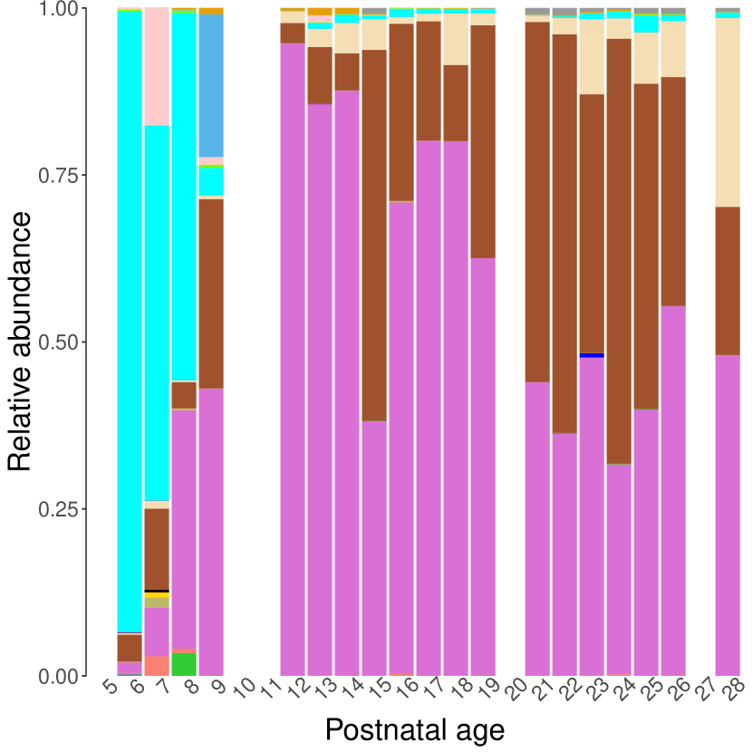
(b)

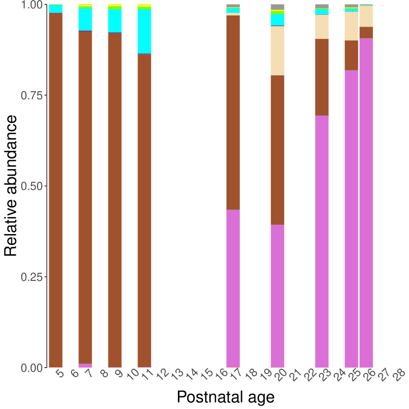
(c)

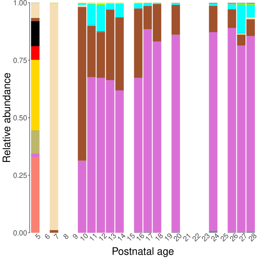
(d)

Figure 1: (a) Histogram of the number of samples collected from each infant. (b)–(d) Example profiles of time-varying compositional data along postnatal age.

Infant neurobehavioral outcomes were measured when the infant reached 36–38 weeks of post-menstrual age or prior to hospital discharge, using the NICU Network Neurobehavioral Scale (NNNS). The NNNS is a standardized assessment of neonatal neurobehavioral outcomes that provides an appraisal of neurological integrity and behavioral function of the normal and at-risk/preterm infant. In particular, the Stress/Abstinence subscale (NSTRESS) measures signs of stress and includes 50 items. Each sign of stress/abstinence is scored as present or absent, and the composite NSTRESS score ranges between 0 and 1. A higher NSTRESS score demonstrates a more stressful behavioral performance. Cong et al. (2017) showed that the composite NSTRESS score is positively associated with painful/stressful experience in preterm infants. Other variables about birth and characteristics of infant included gender, delivery type, premature rupture of membranes (PROM), score for Neonatal Acute Physiology–Perinatal Extension-II (SNAPPE-II), birth weight, and percentage of feeding with mother’s breast milk (%MBM).

To formulate the statistical problem, let ${\bf y}=[y_{1},\ldots,y_{n}]^{\rm T}\in\mathbb{R}^{n}$ be consisting of the observed neurobehavioral outcomes of the preterm infants, i.e., their NNNS scores. Let ${\bf x}_{i}(t)=[x_{i1}(t),\ldots,x_{ip}(t)]^{\rm T}\in\mathbb{S}^{p-1}$ be the gut microbiome compositions from the $i$th infant at time $t$. Here we let $\mathbb{S}^{p-1}=\{[x_{1},\ldots,x_{p}]^{\rm T}\in\mathbb{R}^{p};x_{j}>0,\sum_{j=1}^{p}x_{j}=1.\}$, to denote the $(p-1)$-dimensional positive simplex lying in $\mathbb{R}^{p}$. Let ${\bf X}(t)=[{\bf x}_{1}(t),\ldots,{\bf x}_{n}(t)]^{\rm T}\in\mathbb{R}^{n\times p}$ be the matrix of the functional predictors at time $t$. The observed gut microbiome compositions during the early postnatal period can then be viewed as discrete observations from ${\bf X}(t)$. Also define ${\bf Z}_{c}\in\mathbb{R}^{n\times p_{c}}$, formed by data from the aforementioned time-invariant infant characteristics, e.g., gender, delivery type, among others.

As the main objective is to identify the microbiome markers that are predictive of later infant neurodevelopment, we need to perform a regression analysis to examining how the outcome $y$, the NNNS score, is associated with ${\bf X}(t)$, the gut micorbiome trajectories, while controlling for the infant characteristics collected in ${\bf Z}_{c}$. The fact that ${\bf X}(t)$ is both functional and compositional makes the problem very challenging.

3 Regression with Functional Compositional Predictors

3.1 Linear Log-Contrast Model

We first briefly review the existing regression approaches for dealing with a single set of compositional predictors. Suppose we observed $n$ independent observations of a response variable $y_{i}\in\mathbb{R}$ and a compositional predictor ${\bf x}_{i}=[x_{i1},\ldots,x_{ip}]^{\rm T}$ such that ${\bf x}_{i}\in\mathbb{S}^{p-1}$. Denote ${\bf y}=[y_{1},\ldots,y_{n}]^{\rm T}\in\mathbb{R}^{n}$ as the response vector and ${\bf X}=[{\bf x}_{1},\ldots,{\bf x}_{n}]^{\rm T}\in\mathbb{R}^{n\times p}$as the design matrix.

Ignoring the simplex structure of ${\bf X}$ would lead to parameter identifiablity issue in the linear regression of ${\bf y}$ on ${\bf X}$. One naive “remedy” is to exclude an arbitrary component of the compositional vector in the regression, which, however, leads to a method that is not invariant to the choice of the removed component since it affects both of prediction and selection and consequently makes proper model interpretation and inference difficult. Ever since the pioneer work by John Aitchison (Aitchison, 1982; Aitchison and Bacon-Shone, 1984; Aitchison, 2003) on the statistical treatments of compositional data, the so-called log-contrast model has gained much popularity in a variety of regression problems with compositional predictors. The main idea is to perform a log-ratio transformation of the compositional data, such that the transformed data admit the familiar Euclidean geometry in $\mathbb{R}^{p-1}$. Specifically, for each $i=1,\ldots,n$, let $\widetilde{z}_{ij}=\log(x_{ij}/x_{ir})$, where $r\in\{1,\ldots,p\}$ is a chosen reference level, and $j=1,\ldots,r-1,r+1,\ldots,p$, resulting in $\widetilde{{\bf Z}}_{\bar{r}}=[\widetilde{z}_{ij}]\in\mathbb{R}^{n\times(p-1)}$. Also define $z_{ij}=\log(x_{ij})$ and ${\bf Z}=[z_{ij}]\in\mathbb{R}^{n\times p}$. The linear log-contrast regression model is expressed as

$${\bf y}=\beta_{0}^{*}{\bf 1}_{n}+\widetilde{{\bf Z}}_{\bar{r}}\mbox{\boldmath$\beta$}_{\bar{r}}^{*}+\mbox{\bf e},$$ (1)

where $\beta_{0}^{*}$ is the intercept, $\mbox{\boldmath$\beta$}_{\bar{r}}^{*}\in\mathbb{R}^{p-1}$ is the regression coefficient vector, and $\mbox{\bf e}\in\mathbb{R}^{n}$ is the random error vector with zero mean. Interestingly, although it appears that the model in (1) depends on the choice of the reference level, it in fact admits a symmetric form. By simple algebra, model (1) can be equivalently expressed as

$${\bf y}=\beta_{0}^{*}{\bf 1}_{n}+{\bf Z}\mbox{\boldmath$\beta$}^{*}+\mbox{\bf e},\qquad\mbox{s.t.}\sum_{j=1}^{p}\beta_{j}^{*}=0,$$ (2)

where $\mbox{\boldmath$\beta$}^{*}$ is the regression coefficient vector for design matrix ${\bf Z}$, and ${\bf e}$ and $\beta_{0}^{*}$ are the same as in model (1). It can be showed that $\mbox{\boldmath$\beta$}_{\bar{r}}^{*}\in\mathbb{R}^{p-1}$ is a subvector of a regression coefficient vector $\mbox{\boldmath$\beta$}^{*}\in\mathbb{R}^{p}$ by removing its $r$th component $\beta_{r}^{*}$.

Consequently, in classical regression setups, the least squares estimation under model (1) is equivalent to the constrained least squares estimation under model (2). However, in high dimensional scenarios, i.e., when $p$ is much larger than $n$, the two model formulations could lead to discrepancies in regularized estimation. For example, the two corresponding lasso criteria (Tibshirani, 1996) are no longer equivalent:

$$\min_{\beta_{0},\mbox{\boldmath$\beta$}_{\bar{r}}} \left\{\frac{1}{2n}\|{\bf y}-\beta_{0}{\bf 1}_{n}-\widetilde{{\bf Z}}_{\bar{r}}\mbox{\boldmath$\beta$}_{\bar{r}}\|^{2}+\lambda\|\mbox{\boldmath$\beta$}_{\bar{r}}\|_{1}\right\},$$ (3)

$$\min_{\beta_{0},\mbox{\boldmath$\beta$}} \left\{\frac{1}{2n}\|{\bf y}-\beta_{0}{\bf 1}_{n}-{\bf Z}\mbox{\boldmath$\beta$}\|^{2}+\lambda\|\mbox{\boldmath$\beta$}\|_{1}\right\},\qquad\mbox{s.t.}\sum_{j=1}^{p}\beta_{j}=0,$$ (4)

where $\|\cdot\|$, $\|\cdot\|_{1}$ denote the $\ell_{2}$, $\ell_{1}$ norms, respectively, and $\lambda$ is a tuning parameter controlling the amount of regularization. Although (3) is simpler to compute, clearly its solution and hence its variable selection depend on the choice of the reference component. In contrast, (4) remains to be symmetric in all the $p$ components. Lin et al. (2014) proposed and studied (4) and showed that the estimator admits many desirable properties (Aitchison, 2003).

3.2 Sparse Functional Log-Contrast Regression

In the preterm infant study, the compositional predictors are observed over a continuous domain, i.e., time, and thus they should be treated as functional compositional data. Recall from Section 2 that ${\bf y}\in\mathbb{R}^{n}$ is the response vector, ${\bf X}(t)\in\mathbb{R}^{n\times p}$ the matrix of the functional and compositional predictors at $t$, and ${\bf Z}_{c}\in\mathbb{R}^{n\times p_{c}}$ the matrix of time-invariant control variables. Here to focus on the main idea, we assume ${\bf X}(t)$ is completely observed for $t\in\mathbb{T}$, and the discussion about handling discrete time data is deferred to Section 4.2. Similar as in Section 3.1, we define $\widetilde{{\bf Z}}_{\bar{r}}(t)\in\mathbb{R}^{n\times(p-1)}$, for $r=1,\ldots,p$, and ${\bf Z}(t)=\log({\bf X}(t))\in\mathbb{R}^{n\times p}$.

Motivated by model (2), we propose a functional log-contrast regression model,

$${\bf y}=\beta_{0}^{*}{\bf 1}_{n}+{\bf Z}_{c}\mbox{\boldmath$\beta$}_{c}^{*}+\int_{t\in\mathbb{T}}{\bf Z}(t)\mbox{\boldmath$\beta$}^{*}(t)dt+\mbox{\bf e},\qquad\mbox{s.t. }\mathbf{1}_{p}^{\rm T}\mbox{\boldmath$\beta$}^{*}(t)=0,\,\forall t\in\mathbb{T},$$ (5)

where $\beta_{0}^{*}$ is the intercept, $\mbox{\boldmath$\beta$}_{c}^{*}\in\mathbb{R}^{p_{c}}$ is the regression coefficient vector corresponding to the control variables, $\mbox{\boldmath$\beta$}^{*}(t)=[\beta_{1}^{*}(t),\ldots,\beta_{p}^{*}(t)]^{\rm T}\in\mathbb{R}^{p}$ is the functional regression coefficient vector as a function of $t$, and the remaining terms are defined the same as in model (2). The proposed model allows the compositional predictors to have potentially different effects on the response through $\mbox{\boldmath$\beta$}^{*}(t)$, and their aggregated effects on the response is then given by the integral of ${\bf Z}(t)$ weighted by $\mbox{\boldmath$\beta$}^{*}(t)$ over time. Following Lin et al. (2014), here we adopt the symmetric form of the log-contrast model, in which the zero-sum constraints preserve the simplex structure over time while all the compositional components are treated equally.

To address the problems in the preterm infant study, we consider both sparsity and smoothness of $\mbox{\boldmath$\beta$}^{*}(t)$. First, as it is believed that only a few compositional components are relevant to the prediction of the outcome, we assume the true coefficient curves are sparse, i.e., $s^{*}=|\mathcal{S}|\ll p$, where $\mathcal{S}$ is the index set of the non-zero coefficient curves

$$\mathcal{S}=\{j;\beta_{j}^{*}(t)\neq 0\mbox{ for some }t\in\mathbb{T},j=1,\ldots,p.\}.$$

This sparsity assumption is the basis of component selection and is widely applicable, especially when $p$, the number of compositional components, is large. Second, since the effects of gut microbiome compositions on preterm infant’s neurodevelopment evolves gradually over the postnatal period, we assume the coefficient curves are smooth over $t$, and adopt a truncated basis expansion approach (Ramsay and Silverman, 2005) to bring the infinite dimensional problem to finite dimensions. Specifically, we assume

$$\mbox{\boldmath$\beta$}^{*}(t)=\mathbf{B}^{*}\boldsymbol{\Phi}(t),$$ (6)

where $\mathbf{B}^{*}=[\mbox{\boldmath$\beta$}_{1}^{*},\ldots,\mbox{\boldmath$\beta$}_{p}^{*}]^{\rm T}\in\mathbb{R}^{p\times k}$ is a coefficient matrix, and $\boldsymbol{\Phi}(t)=[\phi_{1}(t),\ldots,\phi_{k}(t)]^{\rm T}\in\mathbb{R}^{k}$ consists of basis with ${\bf J}_{\phi\phi}=\int_{t\in\mathbb{T}}\boldsymbol{\Phi}(t)\boldsymbol{\Phi}^{\rm T}(t)dt$ being a positive definite (p.d.) matrix. Here for simplicity the same set of basis functions is used in the expansion of each $\beta_{j}(t)$, $j=1,\ldots,p$, which usually suffices in practice, and the extension to use different basis for different $\beta_{j}(t)$ is straightforward. There are many choices of the basis functions, e.g., Fourier basis, wavelet basis, and spline basis; see Ramsay and Silverman (2005) for a detailed account on the truncated basis expansion approaches in functional regression.

Some discussions on the number of basis functions are in order. In classical least squares types of estimation, the choice of $k$ usually boils down to a bias-and-variance tradeoff. That is, while larger values of $k$ can lead to a better in-sample estimation at the risk of potential overfitting, smaller values of $k$ result in simpler estimators at the expense of missing interesting local oscillations. The issue can be resolved by echoing regularization, i.e., taking a sufficiently large $k$ to ensure the flexibility of the model and performing regularized estimation to avoid overfitting. From a theoretical perspective, we allow $k$ to grow with the sample size $n$, that is, the complexity of the functional curves that the method can potentially capture may increase when more data become available; see Section 5 for details. We also remark that for a non-parametric treatment, one can assume $\mbox{\boldmath$\beta$}^{*}(t)$ satisfies certain Hölder condition (Tsybakov, 2008) to control the approximate error induced by the basis truncation.

The functional sparsity in $\mbox{\boldmath$\beta$}^{*}(t)$ now amounts to the row-sparsity of the coefficient matrix $\mathbf{B}^{*}$ in (6). The zero-sum constraint on $\mbox{\boldmath$\beta$}^{*}(t)$, i.e., ${\bf 1}_{p}^{\rm T}\mbox{\boldmath$\beta$}^{*}(t)=0$ for all $t\in\mathbb{T}$, is now equivalent to $\mathbf{B}^{*\rm T}{\bf 1}_{p}={\bf 0}$. To see this, note that $\mathbf{1}_{p}^{\rm T}\mbox{\boldmath$\beta$}^{*}(t)=0$ leads to $\int_{t\in\mathbb{T}}{\bf 1}_{p}^{\rm T}\mathbf{B}^{*}\boldsymbol{\Phi}(t)\boldsymbol{\Phi}(t)^{\rm T}({\bf 1}_{p}^{\rm T}\mathbf{B}^{*})^{\rm T}dt={\bf 1}_{p}^{\rm T}\mathbf{B}^{*}{\bf J}_{\phi\phi}({\bf 1}_{p}^{\rm T}\mathbf{B}^{*})^{\rm T}=0$; it follows that $\mathbf{B}^{*\rm T}{\bf 1}_{p}={\bf 0}$ as ${\bf J}_{\phi\phi}$ is p.d.. (The other direction holds trivially.) Further, the integral part in the model becomes

$$\int_{t\in\mathbb{T}}{\bf Z}(t)\mbox{\boldmath$\beta$}^{*}(t)dt =\int_{t\in\mathbb{T}}{\bf Z}(t)\mathbf{B}^{*}\boldsymbol{\Phi}(t)dt$$

$$=\left\{\int_{t\in\mathbb{T}}{\bf Z}(t)({\bf I}_{p}\otimes\boldsymbol{\Phi}(t)^{\rm T})dt\right\}\mbox{vec}(\mathbf{B}^{*\rm T})={\bf Z}\mbox{\boldmath$\beta$}^{*},$$

where, with some abuse of notations, we redefine $\mbox{\boldmath$\beta$}^{*}=[\mbox{\boldmath$\beta$}_{1}^{*\rm T},\ldots,\mbox{\boldmath$\beta$}_{p}^{*\rm T}]^{\rm T}=\mbox{vec}(\mathbf{B}^{*\rm T})\in\mathbb{R}^{pk}$ and

$${\bf Z} =\int_{t\in\mathbb{T}}{\bf Z}(t)({\bf I}_{p}\otimes\boldsymbol{\Phi}(t)^{\rm T})dt=[{\bf Z}_{1},\ldots,{\bf Z}_{p}]\in\mathbb{R}^{n\times(pk)}.$$ (7)

Each $\mbox{\boldmath$\beta$}_{j}^{*}\in\mathbb{R}^{k}$ and ${\bf Z}_{j}\in\mathbb{R}^{n\times k}$ correspond to the coefficient vector and the covariate matrix for the $j$th compositional component, respectively. We remark that ${\bf Z}$ is usually not exactly computed since ${\bf Z}(t)$ may not be fully observed; we defer the discussion to Section 4.2.

The functional model in (5) then becomes a constrained sparse linear regression model

$${\bf y}=\beta_{0}^{*}\mathbf{1}_{n}+{\bf Z}_{c}\mbox{\boldmath$\beta$}_{c}^{*}+{\bf Z}\mbox{\boldmath$\beta$}^{*}+\mbox{\bf e},\qquad\mbox{s.t. }\sum_{j=1}^{p}\mbox{\boldmath$\beta$}_{j}^{*}={\bf 0},$$ (8)

where $\mbox{\boldmath$\beta$}^{*}$ is expected to be sparse accordingly to the row-sparsity of $\mathbf{B}^{*}$. To enable the selection of the compositional components, we therefore propose to conduct model estimation by minimizing a linearly constrained group lasso criterion (Yuan and Lin, 2006),

$$\min_{\beta_{0},\mbox{\boldmath$\beta$}_{c},\mbox{\boldmath$\beta$}}\left\{\frac{1}{2n}\|{\bf y}-\beta_{0}{\bf 1}_{n}-{\bf Z}_{c}\mbox{\boldmath$\beta$}_{c}-{\bf Z}\mbox{\boldmath$\beta$}\|^{2}+\lambda\sum_{j=1}^{p}\|\mbox{\boldmath$\beta$}_{j}\|\right\},\qquad\mbox{s.t.}\sum_{j=1}^{p}\mbox{\boldmath$\beta$}_{j}={\bf 0},$$ (9)

where $\lambda$ is a tuning parameter controlling the amount of regularization. We remark that the group lasso penalty is imposed on the coefficients for each microbiome category to encourage microbe selection.

The proposed estimator possesses several desirable invariance properties (Aitchison, 2003; Lin et al., 2014):

(I) Scale invariance: the estimator is invariant to the transformation ${\bf X}(t)\rightarrow{\bf S}{\bf X}(t)$ where ${\bf S}=\mbox{diag}({\bf s})$ is a diagonal matrix with diagonal elements ${\bf s}=[s_{1},\ldots,s_{n}]^{\rm T}$ and all $s_{i}>0$. That is, it does not matter whether the data vectors are scaled to have a unit sum; the method only cares about the relative proportions. This is simply because ${\bf Z}(t)\mbox{\boldmath$\beta$}(t)=\{\log({\bf X}(t))+\log({\bf s}){\bf 1}_{p}^{\rm T}\}\mbox{\boldmath$\beta$}(t)=\log({\bf X}(t))\mbox{\boldmath$\beta$}(t)$, due to the zero-sum constraints. In fact, this scale invariance continues to hold when the scaling factor ${\bf s}$ changes in time.

(II) Permutation invariance: results of the analysis do not depend on the sequence by which the components are given or labeled.

(III) Subcomposition coherence: if we know in advance that some $\beta_{j}(t)$ curves are zero, the analysis is unchanged if we apply the procedure to the subcompositions formed by the components of ${\bf X}(t)$ corresponding to the other $\beta_{j}(t)$ curves. To see this, suppose $\beta_{j}(t)\equiv 0$ for $j\in\mathcal{S}^{c}$, where $\mathcal{S}^{c}$ is the complement of a set $\mathcal{S}$ on $\{1,\ldots,p\}$. Let ${\bf s}(t)=\{{\bf X}_{\mathcal{S}}(t){\bf 1}_{|\mathcal{S}|}\}^{-1}\in\mathbb{R}^{n}$ be a scaling factor in which the inversion is entrywisely applied, so that $\mbox{diag}({\bf s}(t)){\bf X}_{\mathcal{S}}(t)$ gives the subcompositions formed by the components in $\mathcal{S}$. Then we have

$$\log({\bf X}(t))\mbox{\boldmath$\beta$}(t)= \{\log({\bf X}_{\mathcal{S}}(t))+\log({\bf s}(t)){\bf 1}_{|\mathcal{S}|}^{\rm T}\}\mbox{\boldmath$\beta$}_{\mathcal{S}}(t)$$

$$= \log(\mbox{diag}({\bf s}(t)){\bf X}_{\mathcal{S}}(t))\mbox{\boldmath$\beta$}_{\mathcal{S}}(t).$$

In particular, when there are only two non-zero components, e.g., $\mbox{\boldmath$\beta$}_{1}(t)\neq 0$, $\mbox{\boldmath$\beta$}_{2}(t)\neq 0$ and $\mbox{\boldmath$\beta$}_{j}(t)=0$ for $j=3,\ldots,p$, it is necessarily true that $\mbox{\boldmath$\beta$}_{1}(t)=-\mbox{\boldmath$\beta$}_{2}(t)$ due to the zero-sum constraint. This is neither an unpleasant artifact nor a limitation of the proposed method. This special case can be understood from the above property of subcomposition coherence: the analysis becomes the same as using the subcompositions formed from the first two components of ${\bf X}(t)$; consequently, the two possible log-ratios are exactly opposite to each other, so do their corresponding coefficient curves. Therefore, this feature is consistent with the data structure, as in two-part componsitional data, either part carries exactly the same information.

4 Computation

4.1 Solving and Tuning Constrained Group Lasso

The problem in (9) is convex, and we solve it by an augmented Lagrangian algorithm (Boyd et al., 2011). To save space, details are provided in Section A of Supplementary Materials.

A general way to select the tuning parameters, i.e., the basis dimension $k$ and the group penalty level $\lambda$, is the $K$-fold cross validation (Stone, 1974), which is based on the predictive performance of the models. However, it is well known that the best model for prediction may not coincide with that for variable selection, and in fact, the former often leads to overselection. This phenomenon under our model is revealed in Section 5, where it is shown that consistent component selection shall be based on the zero pattern of a thresholded estimator. Following Fan and Tang (2013) and Lin et al. (2014), we thus also experiment with minimizing a generalized information criterion (GIC) for model selection which favors more sparse models,

$$\textrm{GIC}(\lambda,k)=\log\big{(}\widehat{\sigma}^{2}(\lambda,k)\big{)}+\big{(}s(\lambda,k)-1\big{)}k\log\big{(}\max\{pk+1+p_{c},n\}\big{)}\frac{\log(\log n)}{n},$$

where $\widehat{\sigma}^{2}(\lambda,k)$ is the mean squared error define as $\|{\bf y}-\widehat{\beta}_{0}(\lambda,k){\bf 1}_{n}-{\bf Z}_{c}\widehat{\mbox{\boldmath$\beta$}}_{c}(\lambda,k)-{\bf Z}\widehat{\mbox{\boldmath$\beta$}}(\lambda,k)\|^{2}/n$ with $\widehat{\beta}_{0}(\lambda,k)$, $\widehat{\mbox{\boldmath$\beta$}}_{c}(\lambda,k)$ and $\widehat{\mbox{\boldmath$\beta$}}(\lambda,k)$ being the regularized estimators of regression coefficients, and $s(\lambda,k)$ is the number of nonzero coefficient groups in $\widehat{\mbox{\boldmath$\beta$}}(\lambda,k)$.

4.2 On Discrete Time Observations

So far we have treated the integrated design matrix ${\bf Z}$ defined in (7) as given. In practical situations, however, the functional compositional predictors are most often not observed continuously but at discrete points, so ${\bf Z}$ can not be computed exactly. It is preferable that the induced uncertainty is considered in statistical modeling. In functional regression with a scalar response, Ramsay and Silverman (2005) discussed using truncated basis expansions for both the functional predictor and the functional coefficient curve to convert the infinite dimensional problem to finite dimensional, where truncation can be viewed as a type of regularization. Integrals were approximated by finite Riemann sums with discrete observations. The subsequent methodological development in functional regression has mainly followed along this general strategy, with various choices of basis functions and associated regularization approaches (Morris, 2015). For example, a functional predictor could be expanded by its eigenbasis via a functional principal component analysis, and the coefficient function could be expanded either by the same eigenbasis or by other basis such as wavelet or spline.

Due to the nature of the compositional data, ideally the functional compositions shall be expanded by a multivariate basis that preserves the simplex structure under truncation or other types of regularization, which however, to the best of our knowledge, is not yet available. In essence, a multivariate functional principal component analysis for compositional data, or a joint modeling approach of both the functional compositions and the regression, is needed, which is beyond the scope of the current work.

For the preterm infant study, we take a pragmatic way of lifting the discrete-time data to continuous time. In this study, stool sample of each baby was collected daily whenever available; this resulted in a good coverage rate, with on average 12.2 daily samples for each infant over a 24-day study period. Also, biologists believe that the gut microbiome compositions change continuously over time. As such, we simply apply linear interpolation to obtain continuous time compositional curves. It can be readily seen that the linear interpolation approach amounts to compute ${\bf Z}$ defined in (7) using the trapezoid rule.

Specifically, suppose for each $i=1,\cdots,n$, we observe ${\bf x}_{i}(t)=[x_{i1}(t),\cdots,\allowbreak x_{ip}(t)]^{\rm T}$ at discrete time points $t_{i,v}\in\mathbb{T}=[T_{1},T_{2}]$, for $v=1,\cdots,m_{i}$. That is, different subjects may be observed at different sets of time points in $\mathbb{T}$. Correspondingly, we have

$${\bf z}_{i}(t)=[z_{i1}(t),\cdots,z_{ip}(t)]^{\rm T},\quad t=t_{i,1},\cdots,t_{i,m_{i}},\;i=1,\cdots,n.$$

Recall that ${\bf Z}=\int_{t\in\mathbb{T}}{\bf Z}(t)({\bf I}_{p}\otimes\boldsymbol{\Phi}(t)^{\rm T})dt\in\mathbb{R}^{n\times(pk)}$. Let ${\bf Z}=[{\bf Z}_{1},\cdots,{\bf Z}_{p}]\in\mathbb{R}^{n\times(pk)}$ with ${\bf Z}_{j}=[z_{ijl}]_{n\times k}\in\mathbb{R}^{n\times k}$ for $j=1,\cdots,p$. Adopting linear interpolation, the entries of ${\bf Z}$ are computed using the trapezoid rule as follows,

$$z_{ijl}= \sum_{v=2}^{m_{i}}\big{(}\phi_{l}(t_{i,v-1})z_{ij}(t_{i,v-1})+\phi_{l}(t_{i,v})z_{ij}(t_{i,v})\big{)}\frac{t_{i,v}-t_{i,v-1}}{2}$$

$$+\phi_{l}(t_{i,1})z_{ij}(t_{i,1})(t_{i,1}-T_{0})+\phi_{l}(t_{i,m_{i}})z_{ij}(t_{i,m_{i}})(T_{1}-t_{i,m_{i}}),$$ (10)

for $l=1,\cdots,k$. In what follows, unless otherwise noted, the integrals in the case of discrete data are computed using the above trapezoid rule.

5 Theoretical Perspectives

Here we attempt to provide some theoretical perspectives of two questions of practical concerns: (1) whether it is indeed beneficial to use the linearly constrained formulation rather than a naive baseline formulation, which chooses an arbitrary reference component to perform the log-ratio transformation of the compositional predictors and then proceeds with an unconstrained group lasso regression, and (2) whether the proposed method can accurately identify the relevant compositional predictors.

We first describe the setup. Our analysis is under the setting when the basis expansion in (6) holds and the integrated design matrix ${\bf Z}$ is available. The results are non-asymptotic, where both the number of functional predictors $p$ and the degrees of freedom of the basis functions $k$ are allowed to grow with the sample size $n$. For any $\mbox{\boldmath$\beta$}=[\mbox{\boldmath$\beta$}_{1}^{\rm T},\ldots,\mbox{\boldmath$\beta$}_{p}^{\rm T}]^{\rm T}\in\mathbb{R}^{pk}$, define $\mbox{\boldmath$\beta$}_{\bar{r}}\in\mathbb{R}^{(p-1)k}$ as a subvector of $\beta$ by removing its $r$th component $\mbox{\boldmath$\beta$}_{r}$, for each $r=1,\ldots,p$. Let $\mathcal{J}\subset\{1,\ldots,p\}$ be an index set, and denote $\mbox{\boldmath$\beta$}_{\mathcal{J}}$ be a subvector of $\beta$ consisting of $\mbox{\boldmath$\beta$}_{j}$, $j\in\mathcal{J}$. Denote $\mathcal{J}^{c}$ as the complement of $\mathcal{J}$. Recall that ${\bf X}(t)=[{\bf x}_{1}(t),\ldots,{\bf x}_{n}(t)]^{\rm T}\in\mathbb{R}^{n\times p}$ ${\bf Z}(t)=[z_{ij}(t)]\in\mathbb{R}^{n\times p}$ with $z_{ij}(t)=\log(x_{ij}(t))$, and $\widetilde{{\bf Z}}_{\bar{r}}(t)=[\widetilde{z}_{ij}(t)]\in\mathbb{R}^{n\times(p-1)}$ with $\widetilde{z}_{ij}(t)=\log(x_{ij}(t)/x_{ir}(t))$ for each $r=1,\ldots,p$. Moreover, due to (6), we define $\widetilde{{\bf Z}}_{\bar{r}}=\int_{t\in\mathbb{T}}\widetilde{{\bf Z}}_{\bar{r}}(t)({\bf I}_{p}\otimes\boldsymbol{\Phi}(t)^{\rm T})dt\in\mathbb{R}^{n\times(p-1)k}$ and ${\bf Z}=\int_{t\in\mathbb{T}}{\bf Z}(t)({\bf I}_{p}\otimes\boldsymbol{\Phi}(t)^{\rm T})dt\in\mathbb{R}^{n\times(pk)}$ as in (7). Write $\widetilde{{\bf Z}}_{\bar{r}}=[\widetilde{{\bf Z}}_{\bar{r},1},\ldots,\widetilde{{\bf Z}}_{\bar{r},r-1},\widetilde{{\bf Z}}_{\bar{r},r+1},\ldots,\widetilde{{\bf Z}}_{\bar{r},p}]$ with each $\widetilde{{\bf Z}}_{\bar{r},j}\in\mathbb{R}^{n\times k}$. Write ${\bf Z}=[{\bf Z}_{1},\ldots,{\bf Z}_{p}]$ with each ${\bf Z}_{j}\in\mathbb{R}^{n\times k}$. Let $\mbox{\boldmath$\Psi$}_{\bar{r},j}=\widetilde{{\bf Z}}_{\bar{r},j}^{\rm T}\widetilde{{\bf Z}}_{\bar{r},j}/n$, for $r=1,\ldots,p$, $j=1,\ldots,p$ and $j\neq r$. It boils down to analyze the constrained linear model with grouped predictors in (8). For simplicity, we omit the intercept and the control variables, and write the model as

$${\bf y}={\bf Z}\mbox{\boldmath$\beta$}^{*}+\mbox{\bf e},\qquad\mbox{s.t. }\sum_{j=1}^{p}\mbox{\boldmath$\beta$}_{j}^{*}={\bf 0},$$

where $\mbox{\boldmath$\beta$}^{*}=[\mbox{\boldmath$\beta$}_{1}^{*\rm T},\ldots,\mbox{\boldmath$\beta$}_{p}^{*\rm T}]^{\rm T}\in\mathbb{R}^{pk}$. Recall that $\mathcal{S}=\{j;\mbox{\boldmath$\beta$}_{j}^{*}(t)\neq{\bf 0},j=1,\ldots,p.\}=\{j;\mbox{\boldmath$\beta$}_{j}^{*}\neq{\bf 0},j=1,\ldots,p.\}$, and $s^{*}=|\mathcal{S}|\ll p$.

The proposed constrained group lasso estimator is,

$$\widehat{\mbox{\boldmath$\beta$}}=\arg\min_{\mbox{\boldmath$\beta$}}\left\{\frac{1}{2n}\|{\bf y}-{\bf Z}\mbox{\boldmath$\beta$}\|^{2}+\lambda\sum_{j=1}^{p}\|\mbox{\boldmath$\beta$}_{j}\|\right\},\qquad\mbox{s.t.}\sum_{j=1}^{p}\mbox{\boldmath$\beta$}_{j}={\bf 0}.$$ (11)

This estimator satisfies that $\widehat{\mbox{\boldmath$\beta$}}_{r}=-\sum_{j\neq r}^{p}\widehat{\mbox{\boldmath$\beta$}}_{j}$. Therefore, it holds true that for any $r=1,\ldots,p$,

$$\widehat{\mbox{\boldmath$\beta$}}_{\bar{r}}=\arg\min_{\mbox{\boldmath$\beta$}_{\bar{r}}}\left\{\frac{1}{2n}\|{\bf y}-\widetilde{{\bf Z}}_{\bar{r}}\mbox{\boldmath$\beta$}_{\bar{r}}\|^{2}+\lambda\sum_{j\neq r}^{p}\|\mbox{\boldmath$\beta$}_{j}\|+\lambda\|\sum_{j\neq r}^{p}\mbox{\boldmath$\beta$}_{j}\|\right\}.$$

On the other hand, as to the baseline method, when the $r$th component is choosing as the reference level, the estimator is given by

$$\widetilde{\mbox{\boldmath$\beta$}}_{\bar{r}}=\arg\min_{\mbox{\boldmath$\beta$}_{\bar{r}}}\left\{\frac{1}{2n}\|{\bf y}-\widetilde{{\bf Z}}_{\bar{r}}\mbox{\boldmath$\beta$}_{\bar{r}}\|^{2}+\lambda\sum_{j\neq r}^{p}\|\mbox{\boldmath$\beta$}_{j}\|\right\}.$$ (12)

Our analysis follows and extends the work by Lounici et al. (2011) on group lasso to the case of constrained group lasso in (11) arising from functional compositional data analysis. All the proofs are provided in Section B of Supplementary Materials.

Assumption 1.

The error terms $e_{1},\ldots,e_{n}$ are independently and identically distributed as $\mbox{N}(0,1)$ random variables.

Assumption 2 (Restricted Eigenvalue Condition (RE)).

There exists $\kappa>0$, such that

$$\min\left\{\frac{\|{\bf Z}\mbox{\boldmath$\Delta$}\|}{\sqrt{n}\|\mbox{\boldmath$\Delta$}_{\mathcal{J}}\|}:\right. |\mathcal{J}|\leq s^{*},\mbox{\boldmath$\Delta$}\in\mathbb{R}^{pk}\neq{\bf 0},\sum_{j=1}^{p}\mbox{\boldmath$\Delta$}_{j}={\bf 0},$$

$$\left.\sum_{j\in\mathcal{J}^{c}}\|\mbox{\boldmath$\Delta$}_{j}\|+\min_{j}\|\mbox{\boldmath$\Delta$}_{j}\|\leq 3\sum_{j\in\mathcal{J}}\|\mbox{\boldmath$\Delta$}_{j}\|.\right\}\geq\kappa.$$

Theorem 1 (Error Bounds).

Suppose Assumptions 1–2 hold. Choose

$$\lambda\geq\min_{r}\max_{j\neq r}\frac{2\sigma}{\sqrt{n}}\sqrt{\mbox{tr}(\mbox{\boldmath$\Psi$}_{\bar{r},j})+2\sigma_{\max}(\mbox{\boldmath$\Psi$}_{\bar{r},j})(2q\log(p-1)+\sqrt{kq\log(p-1)})}.$$

Then, with probability at least $1-2(p-1)^{1-q}$, the constrained group lasso estimator $\widehat{\mbox{\boldmath$\beta$}}$ in (11) satisfies that

$$\frac{1}{n}\|{\bf Z}(\widehat{\mbox{\boldmath$\beta$}}-\mbox{\boldmath$\beta$}^{*})\|^{2}\leq\frac{16\lambda^{2}s^{*}}{\kappa^{2}},$$

$$\sum_{j=1}^{p}\|\widehat{\mbox{\boldmath$\beta$}}_{j}-\mbox{\boldmath$\beta$}_{j}^{*}\|+\min_{j}\|\widehat{\mbox{\boldmath$\beta$}}_{j}-\mbox{\boldmath$\beta$}_{j}^{*}\|\leq\frac{16\lambda s^{*}}{\kappa^{2}}.$$

It is interesting to compare with the baseline approach in (12), for which once a baseline $r$ is chosen, its theoretical property mimics that of the regular group lasso model with $p-1$ groups (Lounici et al., 2011). Due to the linear constraints, the restricted set of $\Delta$ in Assumption 2 for which the minimum is taken is smaller than that of the regular group lasso estimator. As such, the condition for the constrained model becomes weaker in general. Also, in Theorem 1, the choice of $\lambda$, which directly impacts the final estimation error rate, is taken as a minimal value over $r$, the choice of the baseline. Therefore, in view of the RE condition and the choice of $\lambda$, our results reveal that the proposed method is capable of achieving the best possible performance of the baseline method under a possibly weaker condition.

Assumption 3 ($\beta$-min Condition).

Choose the same $\lambda$ as in Theorem 1. Assume that

$$\min_{j\in\mathcal{S}}\|\mbox{\boldmath$\beta$}_{j}^{*}\|>\frac{16\lambda s^{*}}{\kappa^{2}}.$$

Corollary 2 (Selection Consistency).

Suppose Assumptions 1–3 hold. Let

$$\widehat{\mathcal{S}}=\{j:\|\widehat{\mbox{\boldmath$\beta$}}_{j}\|>\frac{8\lambda s^{*}}{\kappa^{2}}\}.$$

Then, with probability at least $1-2(p-1)^{1-q}$, we have that $\widehat{\mathcal{S}}=\mathcal{S}$.

Corollary 2 reveals the “overselection” phenomenon due to convex penalization; see, e.g., Wei and Huang (2010). That is, the proposed constrained group lasso estimator in general does not miss important variable groups/components, albeit overselecting some irrelevant ones. As such, a thresholding operation is preferred in order to recovery the correct sparsity pattern exactly. However, the theoretical threshold is not available in practice, as it involves unknown quantities such as $\sigma^{2}$ and $\kappa$. Nevertheless, the results provide guarantee that using the original estimator can avoid false negatives at the expense of some false positives, which is acceptable in many applications.

6 Simulation

We conduct simulation studies to compare the performance of our proposed sparse functional log-contrast regression via constrained group lasso (CGL) in (9), the baseline approach in the form of (12) via group lasso (BGL) in which the reference level is chosen randomly, and the naive approach of group lasso (GL) in which the zero-sum constraints are ignored in (9), and cross sectional method (I) of taking average of observations along time (Average), and cross sectional method (II) of considering the snapshot of the most significant time point (Snapshot).

The compositional data are generated as follows. We first generate $M$ time points within the interval $[0,1]$, i.e., $0=t_{1}<\cdots<t_{M}=1$. For inducing dependence between time points, we consider an autoregressive correlation structure, $\mbox{\boldmath$\Sigma$}_{T}=[\rho_{T}^{|\mu-\nu|}]_{M\times M}$, where $1\leq\mu,\nu\leq M$; for inducing dependence between compositions, we consider a compound symmetry correlation structure, $\mbox{\boldmath$\Sigma$}_{X}=[\rho_{X}^{I(j=j^{\prime})}]_{p\times p}$, where $1\leq j,j^{\prime}\leq p$ and $I(\cdot)$ is the indicator function. The “non-normalized” data for each subject $i$, $i=1,\ldots,n$, are then generated from multivariate normal distribution as ${\bf w}_{i}=[{\bf w}_{i}({t_{1}})^{\rm T},\cdots,{\bf w}_{i}(t_{M})^{\rm T}]^{\rm T}\sim\mbox{N}({\bf 0},\sigma_{X}^{2}(\mbox{\boldmath$\Sigma$}_{T}\otimes\mbox{\boldmath$\Sigma$}_{X}))$, where each ${\bf w}_{i}(t_{\nu})\in\mathbb{R}^{p}$ for $\nu=1,\ldots,M$. Finally, the compositional data are obtained as $x_{ij}(t_{\nu})=\exp(w_{ij}(t_{\nu}))/\sum_{j=1}^{p}\exp(w_{ij}(t_{\nu}))$, for $i=1,\ldots,n$, $j=1,\ldots,p$ and $\nu=1,\ldots,M$. The regression curves $\mbox{\boldmath$\beta$}^{*}(t)$ are generated as $\mathbf{B}^{*}\boldsymbol{\Phi}(t)$, where $\mbox{\boldmath$\Psi$}(t)$ is from a set of cubic spline basis computed using the bs function in the R package splines with $t\in\{t_{1},\ldots,t_{M}\}$ and degrees of freedom set to 5. The first three rows of $\mathbf{B}^{*}$ are set as $[1,0,1,0,-0.5]$, $[0,0,-1,0,1]$ and $[-1,0,0,0,-0.5]$, respectively, and the rest are set to zero. The intercept is set to be $\beta_{0}^{*}=1$ and for simplicity we do not consider additional control. The error terms are generated as independent $\mbox{N}(0,\sigma^{2})$ random variables where $\sigma^{2}$ is set to control the signal to noise ratio (SNR). Finally, the response ${\bf y}$ is generated by model (5), where the integral is computed as in (10). We have experimented with $(n,p)\in\{(50,30),(100,30),(100,100),(100,200)\}$ and parameter settings $M=20$, $\sigma_{X}^{2}=9$, $\rho_{T}\in\{0,0.6\}$, $\rho_{X}=\{0,0.6\}$ and $\mbox{SNR}=\{2,4\}$. The simulation is repeated 100 times under each setting.

The prediction error (Pred) is measured by $\|{\bf y}_{te}-{\bf Z}_{te}\widehat{\mbox{\boldmath$\beta$}}\|^{2}/n_{te}$, computed from an independently generated test sample $({\bf y}_{te};{\bf X}_{te}(t),t\in\{t_{1},\ldots,t_{M}\})$ of size $n_{te}=500$. The estimation error (Est) is measured by $\sum_{j=1}^{p}(\int_{[0,1]}|\widehat{\beta}_{j}(t)-\beta_{j}^{*}(t)|^{2}\,dt)^{1/2}/p$. For variable selection of the compositional components, we report the false positive rate (FPR) and the false negative rate (FNR), based on the sparsity patterns of $\widehat{\mbox{\boldmath$\beta$}}(t)$ and $\mbox{\boldmath$\beta$}^{*}(t)$. We have experimented with both 10-fold cross validation (CV) and GIC for selecting tuning parameters $k$ and $\lambda$. As shown in Corollary 2, a thresholding of the estimator is preferred for the purpose of variable selection, although the ideal threshold is not available in practice. Here with the same spirit and based on empirical evidence, we define the selected index set $\widehat{\mathcal{S}}$ based on the relative magnitudes of the $p$ estimated coefficient curves:

$$\widehat{\mathcal{S}}=\{j;\big{(}\int_{[0,1]}\widehat{\beta}_{j}^{2}(t)\,dt\big{)}^{1/2}/\{\sum_{j=1}^{p}\big{(}\int_{[0,1]}\widehat{\beta}_{j}^{2}(t)\,dt\big{)}^{1/2}\}\geq 1/p,j=1,\cdots,p\}.$$

That is, we only count the components whose relative “energy” exceeds the average $1/p$ as selected.

The simulation results for $(n,p)=(50,30)$ and $(n,p)=(100,200)$ with $\mbox{SNR}=4$ are reported in Tables 1 – 2. The two naive methods, Average and Snapshot perform much worse in prediction than other methods; they tend to miss important variables as seen from their high FNR values. (To save space, we do not show the results of Average and Snapshot with GIC tuning.) In general, CGL shows better predictive and selection performance than both GL and BGL, and in some cases the improvement can even be substantial; (We have also tried the unpenalized least squares estimator, which fails miserably in prediction and hence is omitted.) The BGL method performs the worst among the three. The two tuning methods, CV and GIC, show quite difference behaviors: the former generally yields larger false positive rates and much smaller false negative rates than the latter. Indeed, this is consistent with the theoretical results in Section 5 that the proposed convex regularized estimation approach has a tendency of over-selection when tuned based on optimizing predictive performance. Nevertheless, the CV-tuned estimators rarely miss important components and performs much better in prediction comparing to their GIC tuned counterparts. Therefore, CV may be preferable in practice when one cares more about prediction and can afford some false alarms for the capture of all the relevant signals.

Table 1: Simulation results for $(n,p)=(50,30)$ and $\mbox{SNR}=4$. Reported are the average values over 100 simulation runs, with the standard deviations in parentheses. For better presentation, the values of Est and Pred are multiplied by 10.

$(\rho_{X},\rho_{T})$	Criterion	Method	Est	Pred	FPR (%)	FNR (%)
$(0,0)$	CV	BGL	0.25 (0.01)	0.39 (0.01)	28.85 (1.28)	0.00 (0.00)
		GL	0.23 (0.01)	0.39 (0.01)	27.48 (1.35)	0.00 (0.00)
		CGL	0.23 (0.01)	0.34 (0.01)	29.22 (1.43)	0.00 (0.00)
		Average		2.03 (0.03)	12.00 (1.37)	66.00 (3.45)
		Snapshot		2.11 (0.05)	16.74 (1.77)	53.00 (3.45)
	GIC	BGL	0.33 (0.01)	1.46 (0.06)	4.04 (0.19)	48.00 (3.33)
		GL	0.31 (0.01)	1.44 (0.05)	0.19 (0.08)	52.67 (2.69)
		CGL	0.29 (0.01)	1.24 (0.05)	1.63 (0.24)	20.00 (2.37)
$(0,0.6)$	CV	BGL	0.28 (0.01)	1.27 (0.04)	30.70 (1.48)	0.33 (0.33)
		GL	0.26 (0.01)	1.21 (0.03)	29.04 (1.40)	0.00 (0.00)
		CGL	0.25 (0.01)	1.13 (0.03)	29.67 (1.43)	0.00 (0.00)
		Average		5.58 (0.14)	19.67 (1.96)	34.00 (3.45)
		Snapshot		5.31 (0.10)	23.44 (1.60)	22.67 (1.83)
	GIC	BGL	0.34 (0.01)	4.61 (0.16)	3.74 (0.16)	52.67 (2.60)
		GL	0.31 (0.00)	3.93 (0.12)	0.11 (0.06)	51.67 (2.39)
		CGL	0.31 (0.01)	3.91 (0.17)	1.52 (0.24)	23.67 (2.19)
$(0.6,0)$	CV	BGL	0.25 (0.01)	0.15 (0.01)	29.26 (1.35)	0.00 (0.00)
		GL	0.24 (0.01)	0.16 (0.00)	29.93 (1.42)	0.00 (0.00)
		CGL	0.23 (0.01)	0.14 (0.00)	29.07 (1.22)	0.00 (0.00)
		Average		0.80 (0.01)	14.63 (1.70)	57.33 (3.52)
		Snapshot		0.85 (0.02)	16.70 (1.73)	57.00 (3.29)
	GIC	BGL	0.34 (0.01)	0.65 (0.02)	3.81 (0.19)	56.33 (2.67)
		GL	0.32 (0.01)	0.62 (0.02)	0.19 (0.08)	59.33 (2.25)
		CGL	0.30 (0.01)	0.54 (0.02)	1.63 (0.22)	22.67 (2.22)
$(0.6,0.6)$	CV	BGL	0.29 (0.01)	0.53 (0.02)	33.52 (1.38)	0.33 (0.33)
		GL	0.26 (0.01)	0.49 (0.02)	30.22 (1.31)	0.00 (0.00)
		CGL	0.25 (0.01)	0.45 (0.01)	30.37 (1.44)	0.00 (0.00)
		Average		2.02 (0.04)	22.81 (1.89)	26.33 (2.81)
		Snapshot		2.10 (0.03)	22.85 (1.60)	25.67 (1.76)
	GIC	BGL	0.35 (0.01)	1.85 (0.06)	3.81 (0.15)	53.67 (2.59)
		GL	0.32 (0.00)	1.69 (0.05)	0.11 (0.06)	57.67 (2.00)
		CGL	0.31 (0.01)	1.52 (0.06)	1.74 (0.23)	25.00 (2.24)

Table 2: Simulation results for $(n,p)=(100,200)$ and $\mbox{SNR}=4$. The layout is the same as in Table 1.

$(\rho_{X},\rho_{T})$	Criterion	Method	Est	Pred	FPR (%)	FNR (%)
$(0,0)$	CV	BGL	0.04 (0.00)	0.31 (0.01)	15.28 (0.48)	0.00 (0.00)
		GL	0.04 (0.00)	0.31 (0.01)	15.27 (0.48)	0.00 (0.00)
		CGL	0.04 (0.00)	0.29 (0.00)	15.57 (0.51)	0.00 (0.00)
		Average		1.98 (0.03)	3.04 (0.41)	73.33 (3.11)
		Snapshot		1.99 (0.03)	4.82 (0.64)	59.33 (3.20)
	GIC	BGL	0.05 (0.00)	1.45 (0.05)	0.51 (0.01)	44.00 (3.07)
		GL	0.04 (0.00)	1.33 (0.05)	0.01 (0.01)	46.33 (2.88)
		CGL	0.04 (0.00)	1.13 (0.05)	0.19 (0.03)	11.67 (1.73)
$(0,0.6)$	CV	BGL	0.04 (0.00)	1.02 (0.02)	16.26 (0.51)	0.00 (0.00)
		GL	0.04 (0.00)	0.97 (0.02)	15.62 (0.52)	0.00 (0.00)
		CGL	0.04 (0.00)	0.94 (0.02)	16.32 (0.50)	0.00 (0.00)
		Average		5.41 (0.10)	7.17 (0.70)	27.00 (2.71)
		Snapshot		5.14 (0.10)	6.57 (0.56)	27.67 (1.26)
	GIC	BGL	0.05 (0.00)	4.15 (0.16)	0.51 (0.01)	43.00 (3.01)
		GL	0.04 (0.00)	3.44 (0.12)	0.01 (0.01)	42.67 (2.92)
		CGL	0.04 (0.00)	3.57 (0.15)	0.10 (0.02)	16.00 (1.92)
$(0.6,0)$	CV	BGL	0.04 (0.00)	0.12 (0.00)	14.78 (0.49)	0.00 (0.00)
		GL	0.04 (0.00)	0.12 (0.00)	15.44 (0.61)	0.00 (0.00)
		CGL	0.04 (0.00)	0.12 (0.00)	15.07 (0.55)	0.00 (0.00)
		Average		0.80 (0.01)	5.14 (0.68)	58.33 (3.80)
		Snapshot		0.81 (0.01)	4.30 (0.49)	61.67 (2.82)
	GIC	BGL	0.05 (0.00)	0.55 (0.02)	0.53 (0.01)	39.00 (3.39)
		GL	0.04 (0.00)	0.47 (0.02)	0.02 (0.01)	36.33 (3.22)
		CGL	0.04 (0.00)	0.41 (0.02)	0.15 (0.03)	9.67 (1.79)
$(0.6,0.6)$	CV	BGL	0.04 (0.00)	0.41 (0.01)	16.21 (0.50)	0.00 (0.00)
		GL	0.04 (0.00)	0.40 (0.01)	15.30 (0.55)	0.00 (0.00)
		CGL	0.04 (0.00)	0.39 (0.01)	15.59 (0.50)	0.00 (0.00)
		Average		2.03 (0.03)	7.35 (0.63)	16.67 (2.25)
		Snapshot		2.09 (0.04)	7.62 (0.67)	27.33 (1.29)
	GIC	BGL	0.05 (0.00)	1.76 (0.06)	0.52 (0.01)	48.33 (2.93)
		GL	0.04 (0.00)	1.46 (0.05)	0.01 (0.01)	47.33 (2.73)
		CGL	0.04 (0.00)	1.40 (0.06)	0.15 (0.03)	17.00 (1.98)

Figure 2 show boxplots of prediction errors from CV tuning for $\mbox{SNR}=4$. (The case of $\mbox{SNR}=2$ is reported in Section C of Supplementary Materials; we do note include Average and Snapshot methods as they perform much worse.) The performance of all methods deteriorates when the SNR becomes smaller, the between-component correlation becomes smaller, or the between-time correlation becomes stronger. Small between-component correlation causes the presence of a few dominating compositional components due to the unit-sum constraints, while large between-time correlation makes the functional compositions smooth over time and consequently makes it hard to distinguish the relevant components from the others.

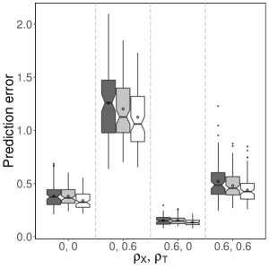
(a) $n=50,p=30$

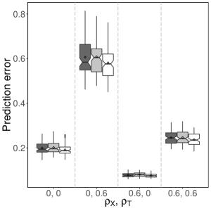
(b) $n=100,p=30$

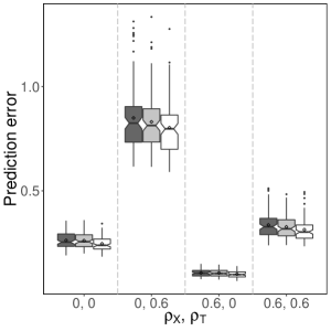
(c) $n=100,p=100$

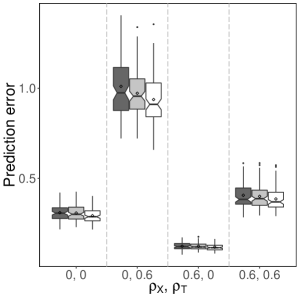
(d) $n=100,p=200$

Figure 2: Boxplots of prediction errors for various simulation settings with $\mbox{SNR}=4$. The dark grey, light grey and white colors correspond to three different estimation methods BGL, GL and CGL, respectively.

7 Linking Microbiome Trajectories to Neurobehavioral Outcomes

Recall that our main objective is to identify the microbiome markers that are predictive of later infant neurodevelopment as measured by NNNS. This predictive association, if proven true, can provide supporting evidence to the claim that the stressful early life experience of preterm infants is imprinting gut microbiome by the regulation of the brain-gut axis. We tackle the problem with the functional log-contrast regression model in (5), in which the composite NSTRESS score serves as the response variable, the gut microbiome observed during the early postnatal period serves as the functional compositional predictors, and the infant characteristics listed in Table 3 below serve as the time-invariate control variables. We apply the proposed CGL approach for model estimation and compositional component selection. The cubic spline basis is used, and the tuning of the degrees of freedom $k$ as well as the sparsity parameter $\lambda$ is done using cross validation.

Our approach is able to identify four bacteria categories at the order level that are associated with the neurobehavioral outcome of infant, after controlling for the effects of several infant characteristics. Before we discuss the selected microbiome markers, let’s first focus on the effects of the control variables. Table 3 shows the estimated coefficients of the control variables along with some descriptive statistics. It is seen that the neurobehavioral outcome is better (i.e., NSTRESS is small) for infants with larger birth weight, smaller SNAPE-II score and more mother’s breast milk for feeding. Regarding the delivery of infant, vaginal delivery and the absence of premature rupture of membranes are associated with better neurobehavioral development. These interesting and intuitive results are consistent with existing literature (Neu and Rushing, 2011; Feldman and Eidelman, 2003). The analysis also shows that female infants tend to perform slightly better than male, after accounting for other effects.

Table 3: Descriptive statistics of infant characteristics and their estimated coefficients from fitting the sparse functional log-contrast regression. Values of estimated coefficient are multiplied by 100.

Numerical variable	Mean (sd)	Estimated coefficient
Birth weight (in gram)	1451.7 (479.3)	$-0.003$
SNAPE-II	9.3 (10.6)	$0.122$
%MBM	61.8 (29.9)	$-9.79$
Binary variable	Percentage of ones
Gender (female = 1)	50.0%	$-0.065$
PROM (yes = 1)	44.1%	$3.11$
Delivery type (vaginal =1)	35.3%	$-5.43$

The estimated functional effects of the four selected bacteria categories are shown in the four panels of Figure 3, respectively. In each panel, the lower part shows the estimated functional effects of a category over time (between 5 and 28 days of postnatal age), and the upper part attempts to show directly from raw data how this category changes over time for infants with high, medium, or low “adjusted” NSTRESS score, obtained by subtracting the estimated effects of the control variables and other selected bacteria categories from the observed NSTRESS scores. Specifically, we construct smoothed curves of log-compositions of each selected category for three clusters of infants (using locally weighted scatterplot smoothing). For each category, the clusters are based on the percentiles of its “adjusted” NSTRESS score. The curve with its 90% confidence band is shown in red for the high group, i.e., infants with the upper one third of the adjusted scores, in blue for the medium group, i.e., infants with the middle one third of the adjusted scores, and in green for the low group, i.e., infants with the lower one third of the adjusted scores. As an example, for category 1, the red curve increases in the beginning to be above the other two curves and then becomes mostly below them in the later stage. This suggests that the time-varying effect of category 1 on the NSTRESS score is first positive and then negative, which is clearly reflected by the estimated functional effects. Similarly for the other three selected categories, the patterns of the estimated effects agree well with those of the observed data. This verifies visually that our proposed model and the estimation approach yield sensible results.

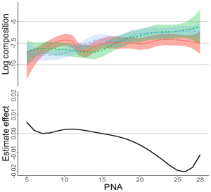
(a) Category 1

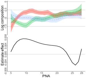
(b) Category 9

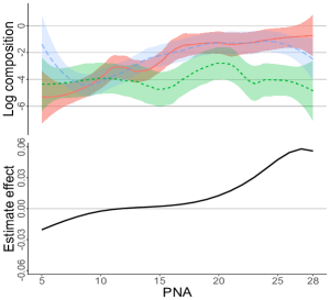
(c) Category 10

(d) Category 19

Figure 3: Estimated effects of the four selected bacteria categories at the order level over infant’s postnatal age (PNA) of 5 to 28 days. In each sub-graph, the upper panel shows how this category changes over time for three clusters of infants. For each category, the clusters are based on the percentiles of its partial residuals, obtained by subtracting the estimated effects of the control variables and other selected bacteria categories from the observed NSTRESS scores. The curve with its 90% confidence band is shown in red for the high group, in blue for the medium group, and in green for the low group.

To access the stability of the results, we have generated 100 bootstrap samples and used the same cross validation procedure to select the best models. The results are show in Figure 4. The signs of the coefficients of the control variables are quite stable, except for the gender and SNAPE-II variables; this shows that these two variables may not have much effect on the outcome when conditioning on other terms in the model. For each control variable, the sign with the higher proportion among its 100 bootstrap estimates agrees with that of the estimate from fitting the original data, except for the gender. Furthermore, the top four categories with the highest proportions of being selected in bootstrap coincide with the categories selected from fitting the original data. Categories 10 and 19 are selected about 90% of the times, while 9 and 1 are selected more than 70% and 60% of the times, respectively.

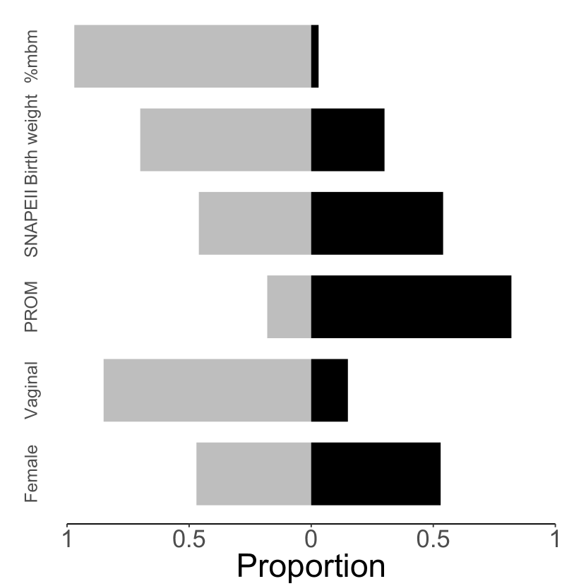
(a)

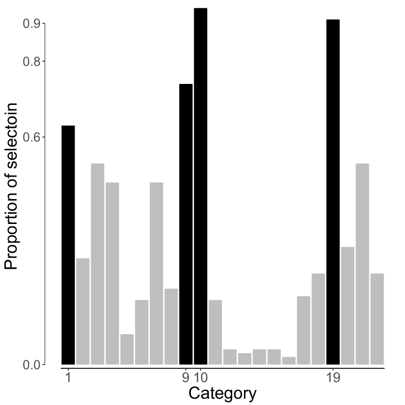
(b)

Figure 4: Selection results from 100 bootstrap samples. (a) Proportions of the signs of the estimated coefficients of the control variables. Proportions of positive signs are shown as black blocks to the right, and those of negative signs are shown as light gray blocks to the left. (b) Proportions of selecting the 22 bacteria categories at the order level. The bars of the four selected categories from fitting the original data are colored in black.

Category 10 consists of Clostridiales, which are an order of bacteria belonging to the phylum Firmicutes. Studies showed that infants fed with mother’s milk had significantly higher abundance in Clostridiales (Cong et al., 2016). Clostridiales are generally regarded as hallmarks of a healthy gut; it can be a sign of infection when their subtypes such as Eubacteria die off in the large intestine. Our results show that controlling for other effects in the model, the effect of Clostridiales on the stress score switches from negative to positive during the postnatal days from 5 to 28. Category 9 consists of Lactobacillales, or lactic acid bacteria (LAB), another order of bacteria belonging to the phylum Firmicutes. These bacteria are usually found in decomposing plants and milk products; they are considered beneficial and produce organic acids such as lactic acid from carbohydrates. Our analysis shows that controlling for the other effects in the model, higher LAB proportions are associated with higher stress scores for a period of time during the early postnatal days. Both Clostridiales and LAB belong to phylum Firmicutes, which make up the largest portion of the human gut microbiome, and the abundance of Firmicutes has been shown to be associated with inflammation and obesity Clarke et al. (2012); Boulangé et al. (2016). Category 19 consists of Enterobacteriales, an order of gram-negative bacteria. They are responsible for various infections such as bacteremia, lower respiratory tract infections, skin infections, etc. Category 1 consists of other unclassified bacteria. The functional regression analysis presented here may lead to a better understanding of how the trajectories of gut microbiome during early postnatal stage impact neurobehavioral outcomes of infants through the gut-brain axis.

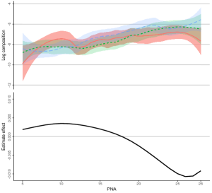
(a) Genus 1

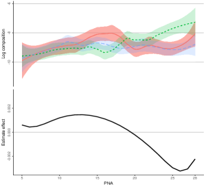
(b) Genus 20

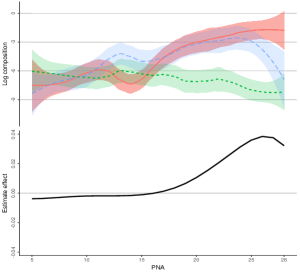
(c) Genus 38

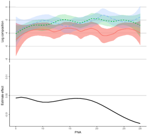
(d) Genus 48

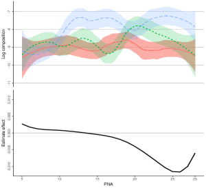
(e) Genus 55

Figure 5: Estimated effects of the five selected bacteria categories at the genus level over infant’s postnatal age (PNA) of 5 to 28 days. The layout is the same as in Figure 3.

We also repeat the analysis on a lower level taxon, i.e., the genus level. Five out of $p=62$ genera are selected, and their estimated functional effects are shown in the five panels of Figure 5. The tendency of the estimated effects adequately reflects those of the observed data and the results are consistent with previous study on the order level. In particular, the five selected genera all belong to the four selected order categories; see Table 4. Genus 38 comprises genus Veillonella, belonging to the order Clostridiales. Veillonella have been implicated as pathogens; they are often associated with oral, central nervous system and various soft tissue infections. Our results show that controlling for the other effect in the model, the effect of Veillonella on the stress score works similarly to that of Clostridiales, switching from negative to positive. Genus 20 consists of Enterococcus, which is an large genus of bacteria belonging to the order LAB. In humans, E. faecalis and E. faecium are the most abundant species of this genus found in fecal content, comprising up to 1% of the adult intestinal microbiota. Although utilization of Enterococci as probiotics has been under controversial discussion, enterococcal strains such as E. faecium SF68 and E. faecalis Symbio-flor have been marketed as probiotics for decades without incidence and with very few reported adverse events (Franz et al., 2011). On the other aspect, Enterococci is also important nosocomial pathogens that cause bacteraemia, endocarditis and other infections. Same as LAB, controlling for the other effect in the model, our results show that higher Enterococcus proportions are associated with higher stress scores for a period of time during the early postnatal days. Genus 55 is Shigella, belonging to the order Enterobacteriales. Shigella is considered as pathogen causing shigellosis. The main sign of shigella infection is diarrhea, which often is bloody. However, shigellosis rarely affects infants during the first month of life. Even in highly endemic areas neonatal shigellosis is exceedingly uncommon (Haltalin, 1967). Our analysis shows that controlling for the other effects in the model, the effect of Shigella changes from positive to negative during early postnatal days. Genus 48 consists of other unclassified genera of bacteria that belongs to the order Enterobacteriales. Genus 1 consists of other unclassified bacteria.

Table 4: Comparison of selection of microbiome markers between order level and genus level.

Order level	Genus level
1: Others	1: Others
9: Lactobacillales Produce organic acids such as lactic acid from carbohydrates.	20: Enterococcus It’s used as probiotics in humans; It’s considered as pathogens that cause bacteraemia, endocarditis and other infections.
10: Clostridiales It’s generally regarded as hallmarks of a healthy gut; It’s a sign of infection when their subtypes such as Eubacteria die off in the large intestine.	38: Veillonella It’s implicated as pathogens; It’s associated with oral infections and various soft tissue infections.
19: Enterobacteriales It’s responsible for various infections such as bacteremia, lower respiratory tract infections, skin infections, etc.	55: Shigella It’s considered as pathogen causing shigellosis; Shigellosis is exceedingly uncommon for infants during the first month of life 48: Others

8 Discussion

We have attempted a functional log-contrast regression approach to identify trajectories of gut microbiome components during early postnatal stage that are associated with later neurobehavioral outcomes of pre-term infants. There are several directions for future research to address the limitations of the current work. The results on order and genus levels only give a general idea of how the microbial communities effect health outcomes, to fully decipher their roles further analysis on species level or even operational taxonomic unit (OTU) is needed. The data analysis can benefit from extending the model to consider potential interactions between the control variables and the gut microbiome, as it is possible, for example, that the effects of certain microbiome markers differ for male and female infants. Extensions to binary outcome or mixture model setup are interesting and could be widely applicable; indeed, it is of interest to see whether there exists a subgroup structure among the preterm infants. To take into account the uncertainty due to discrete observations, it is urgent to develop smoothing or dimension reduction methods such as multivariate functional principal component analysis for compositional data observed discretely over time. A joint modeling approach of both the regression and the functional compositions themselves may also be fruitful.

Supplemental Materials

Appendix A Computational Algorithm

We consider an estimation criterion that is slightly more general than (9) in the main paper,

$$\min_{\beta_{0},\mbox{\boldmath$\beta$}_{c},\mbox{\boldmath$\beta$}}\left\{\frac{1}{2n}\|{\bf y}-\beta_{0}{\bf 1}_{n}-{\bf Z}_{c}\mbox{\boldmath$\beta$}_{c}-{\bf Z}\mbox{\boldmath$\beta$}\|^{2}+\lambda\sum_{j=1}^{p}\|{\bf W}_{j}\mbox{\boldmath$\beta$}_{j}\|\right\},\mbox{s.t.}\sum_{j=1}^{p}{\bf A}_{j}\mbox{\boldmath$\beta$}_{j}={\bf b},$$

where each ${\bf W}_{j}\in\mathbb{R}^{k\times k}$ is invertable, e.g., a diagonal matrix with positive diagonal elements, and the linear constraints, with choices of conformable ${\bf A}_{j}$s and ${\bf b}$, remain feasible, i.e., $\{\mbox{\boldmath$\beta$};\sum_{j=1}^{p}{\bf A}_{j}\mbox{\boldmath$\beta$}_{j}={\bf b}\}\neq\emptyset$. The problem is convex and can be solved by an augmented Lagrangian algorithm (Boyd et al., 2011).

To derive the algorithm, we first construct the scaled augmented Lagrangian function

$$L(\mbox{\boldmath$\beta$}_{0c},\mbox{\boldmath$\beta$};\mbox{\boldmath$\alpha$},\mu)= \frac{1}{2n}\|{\bf y}-\beta_{0}{\bf 1}_{n}-{\bf Z}_{c}\mbox{\boldmath$\beta$}_{c}-{\bf Z}\mbox{\boldmath$\beta$}\|^{2}$$

$$+\frac{\mu}{2}\|\sum_{j=1}^{p}{\bf A}_{j}\mbox{\boldmath$\beta$}_{j}-{\bf b}+\mbox{\boldmath$\alpha$}\|^{2}+\lambda\sum_{j=1}^{p}\|{\bf W}_{j}\mbox{\boldmath$\beta$}_{j}\|,$$

where $\mu>0$ is a prespecified penalty parameter, $\mbox{\boldmath$\alpha$}\in\mathbb{R}^{k}$ is the scaled Lagrange multiplier, and $\mbox{\boldmath$\beta$}_{0c}=(\beta_{0}^{\rm T},\mbox{\boldmath$\beta$}_{c}^{\rm T})^{\rm T}$ collects the unpenalized coefficients.

The algorithm alternates between two steps, a primal step and a dual step, until convergence. Let $\ell=0,1,...$ denote the iteration number. The primal step minimizes $L(\mbox{\boldmath$\beta$}_{0c},\mbox{\boldmath$\beta$};\mbox{\boldmath$\alpha$},\mu)$ with respect to $(\mbox{\boldmath$\beta$}_{0c},\mbox{\boldmath$\beta$})$: $\big{(}\mbox{\boldmath$\beta$}_{0c}^{\ell+1},\mbox{\boldmath$\beta$}^{\ell+1}\big{)}\leftarrow\min_{\mbox{\boldmath$\beta$}_{0c},\mbox{\boldmath$\beta$}}\{L(\mbox{\boldmath$\beta$}_{0c},\mbox{\boldmath$\beta$};\mbox{\boldmath$\alpha$}^{\ell},\mu)\}$. The problem is equivalent to a standard group lasso problem, for which many algorithms are available (Huang et al., 2012). To see this, consider

$$\arg\min_{\mbox{\boldmath$\beta$}}\left\{\frac{1}{2n}\|{\bf y}-{\bf Z}\mbox{\boldmath$\beta$}\|^{2}+\frac{\mu}{2}\|\sum_{j=1}^{p}{\bf A}_{j}\mbox{\boldmath$\beta$}_{j}-{\bf b}+\mbox{\boldmath$\alpha$}^{\ell}\|^{2}+\lambda\sum_{j=1}^{p}\|{\bf W}_{j}\mbox{\boldmath$\beta$}_{j}\|\right\}.$$

Here we have omitted the intercept term and the control variables as they can be treated as a group with zero penalty. Define ${\bf A}=({\bf A}_{1},\ldots,{\bf A}_{p})$, $\widetilde{\mbox{\boldmath$\beta$}}_{j}={\bf W}_{j}\mbox{\boldmath$\beta$}_{j}$, and $\widetilde{\mbox{\boldmath$\beta$}}={\bf W}\mbox{\boldmath$\beta$}=\mbox{diag}({\bf W}_{1},\ldots,{\bf W}_{p})\mbox{\boldmath$\beta$}$. Then the objective can be expressed in terms of $\widetilde{\mbox{\boldmath$\beta$}}$ as

$$\frac{1}{2n}\widetilde{\mbox{\boldmath$\beta$}}^{\rm T}({\bf W}^{-1})^{\rm T}({\bf Z}^{\rm T}{\bf Z}+n\mu{\bf A}^{\rm T}{\bf A}){\bf W}^{-1}\widetilde{\mbox{\boldmath$\beta$}}$$

$$-\frac{1}{n}({\bf y}^{\rm T}{\bf Z}+n\mu({\bf b}-\mbox{\boldmath$\alpha$}^{\ell})^{\rm T}{\bf A}){\bf W}^{-1}\widetilde{\mbox{\boldmath$\beta$}}+\lambda\sum_{j=1}^{p}\|\widetilde{\mbox{\boldmath$\beta$}}_{j}\|.$$

The dual step updates $\alpha$ as $\mbox{\boldmath$\alpha$}^{\ell+1}\leftarrow\mbox{\boldmath$\alpha$}^{\ell}+\sum_{j=1}^{p}{\bf A}_{j}\mbox{\boldmath$\beta$}_{j}^{\ell+1}-{\bf b}$. To speed up computation, $\mu$ can be set to slowly increase along iterations (Boyd et al., 2011).

The optimization procedure for any fixed $\lambda$ is summarized in Algorithm 1. When the model is fitted for a sequence of $\lambda$ values, a warm start strategy is adopted, i.e., the solution for the previous $\lambda$ value is used as the initial value for the next one.

Algorithm 1

Initialize $\mbox{\boldmath$\alpha$}^{0}\geq{\bf 0}$, $\mu^{0}\geq 0$. Choose $\rho>1$, e.g., $\rho=1.05$. Choose convergence thresholds $\epsilon_{1}>0$ and $\epsilon_{2}>0$, e.g., $\epsilon_{1}=\epsilon_{2}=10^{-4}$. Set $\ell\leftarrow 0$.

repeat • Primal step: $\big{(}\mbox{\boldmath$\beta$}_{0c}^{\ell+1},\mbox{\boldmath$\beta$}^{\ell+1}\big{)}\leftarrow\min_{\mbox{\boldmath$\beta$}_{0c},\mbox{\boldmath$\beta$}}\{L(\mbox{\boldmath$\beta$}_{0c},\mbox{\boldmath$\beta$};\mbox{\boldmath$\alpha$}^{\ell},\mu^{\ell})\}$. • Dual step: $\mbox{\boldmath$\alpha$}^{\ell+1}\leftarrow(\mbox{\boldmath$\alpha$}^{\ell}+\sum_{j=1}^{p}{\bf A}_{j}\mbox{\boldmath$\beta$}_{j}^{\ell+1}-{\bf b})/\rho$. • $\mu^{\ell+1}\leftarrow\rho\mu^{\ell}$. • $\ell\leftarrow\ell+1$.

until convergence, i.e., $\big{(}\|\mbox{\boldmath$\beta$}_{0c}^{\ell+1}-\mbox{\boldmath$\beta$}_{0c}^{\ell}\|^{2}+\|\mbox{\boldmath$\beta$}^{\ell+1}-\mbox{\boldmath$\beta$}^{\ell}\|^{2}\big{)}/\big{(}\|\mbox{\boldmath$\beta$}_{0c}^{\ell}\|^{2}+\|\mbox{\boldmath$\beta$}^{\ell}\|^{2}\big{)}\leq\epsilon_{1}$ and $\|\sum_{j=1}^{p}{\bf A}_{j}\mbox{\boldmath$\beta$}_{j}^{\ell+1}-{\bf b}\|^{2}\leq\epsilon_{2}$.

return $\widehat{\mbox{\boldmath$\beta$}}_{0c}=\mbox{\boldmath$\beta$}_{0c}^{\ell}$ and $\widehat{\mbox{\boldmath$\beta$}}=\mbox{\boldmath$\beta$}^{\ell}$.

Appendix B Proofs

We study the properties of the constrained group lasso estimator,

$$\widehat{\mbox{\boldmath$\beta$}}=\arg\min_{\mbox{\boldmath$\beta$}}\left\{\frac{1}{2n}\|{\bf y}-{\bf Z}\mbox{\boldmath$\beta$}\|^{2}+\lambda\sum_{j=1}^{p}\|\mbox{\boldmath$\beta$}_{j}\|\right\},\qquad\mbox{s.t.}\sum_{j=1}^{p}\mbox{\boldmath$\beta$}_{j}={\bf 0}.$$ (13)

as define in (11) of the main paper. For the sake of completeness, we reproduce the theorems in the main paper.

Theorem 3 (Error Bounds).

Suppose Assumptions 1–2 presented in the main paper hold. Choose

$$\lambda\geq\min_{r}\max_{j\neq r}\frac{2\sigma}{\sqrt{n}}\sqrt{\mbox{tr}(\mbox{\boldmath$\Psi$}_{\bar{r},j})+2\sigma_{\max}(\mbox{\boldmath$\Psi$}_{\bar{r},j})(2q\log(p-1)+\sqrt{kq\log(p-1)})}.$$

Then, with probability at least $1-2(p-1)^{1-q}$, the constrained group lasso estimator $\widehat{\mbox{\boldmath$\beta$}}$ in (13) satisfies that

$$\frac{1}{n}\|{\bf Z}(\widehat{\mbox{\boldmath$\beta$}}-\mbox{\boldmath$\beta$}^{*})\|^{2}\leq\frac{16\lambda^{2}s^{*}}{\kappa^{2}},$$ (14)

$$\sum_{j=1}^{p}\|\widehat{\mbox{\boldmath$\beta$}}_{j}-\mbox{\boldmath$\beta$}_{j}^{*}\|+\min_{j}\|\widehat{\mbox{\boldmath$\beta$}}_{j}-\mbox{\boldmath$\beta$}_{j}^{*}\|\leq\frac{16\lambda s^{*}}{\kappa^{2}}.$$ (15)

Corollary 4 (Selection Consistency).

Suppose Assumptions 1–3 presented in the main paper hold. Let

$$\widehat{\mathcal{S}}=\{j:\|\widehat{\mbox{\boldmath$\beta$}}_{j}\|>\frac{8\lambda s^{*}}{\kappa^{2}}\}.$$

Then, with probability at least $1-2(p-1)^{1-q}$, we have that $\widehat{\mathcal{S}}=\mathcal{S}$.

Proof of Theorem 3.

For all $\mbox{\boldmath$\beta$}=[\mbox{\boldmath$\beta$}_{1}^{\rm T},\ldots,\mbox{\boldmath$\beta$}_{p}^{\rm T}]^{\rm T}\in\mathbb{R}^{pk}$, $\sum_{j=1}^{p}\mbox{\boldmath$\beta$}_{j}={\bf 0}$, it holds that

$$\frac{1}{n}\|{\bf y}-{\bf Z}\widehat{\mbox{\boldmath$\beta$}}\|^{2}+2\lambda\sum_{j=1}^{p}\|\widehat{\mbox{\boldmath$\beta$}}_{j}\|\leq\frac{1}{n}\|{\bf y}-{\bf Z}\mbox{\boldmath$\beta$}\|^{2}+2\lambda\sum_{j=1}^{p}\|\mbox{\boldmath$\beta$}_{j}\|,$$

by the optimality of the constrained group lasso estimator $\widehat{\mbox{\boldmath$\beta$}}$. Using ${\bf y}={\bf Z}\mbox{\boldmath$\beta$}^{*}+{\bf e}$, we have that

$$\frac{1}{n}\|{\bf Z}(\widehat{\mbox{\boldmath$\beta$}}-\mbox{\boldmath$\beta$}^{*})\|^{2}\leq\frac{1}{n}\|{\bf Z}(\mbox{\boldmath$\beta$}-\mbox{\boldmath$\beta$}^{*})\|^{2}+\frac{2}{n}{\bf e}^{\rm T}{\bf Z}(\widehat{\mbox{\boldmath$\beta$}}-\mbox{\boldmath$\beta$})+2\lambda\sum_{j=1}^{p}(\|\mbox{\boldmath$\beta$}_{j}\|-\|\widehat{\mbox{\boldmath$\beta$}}_{j}\|).$$ (16)

We first bound the stochastic term ${\bf e}^{\rm T}{\bf Z}(\widehat{\mbox{\boldmath$\beta$}}-\mbox{\boldmath$\beta$})$. Due to the zero-sum constrains, it is important to realize that for any $r=1,\ldots,p$,

$${\bf e}^{\rm T}{\bf Z}(\widehat{\mbox{\boldmath$\beta$}}-\mbox{\boldmath$\beta$})={\bf e}^{\rm T}\widetilde{{\bf Z}}_{\bar{r}}(\widehat{\mbox{\boldmath$\beta$}}_{\bar{r}}-\mbox{\boldmath$\beta$}_{\bar{r}}).$$

The following tail bound is from Lemma A.1 in Lounici et al. (2011).

Lemma 5.

Let ${\bf v}=[v_{1},\ldots,v_{n}]^{\rm T}\neq{\bf 0}$, $\eta_{{\bf v}}=\sum_{i=1}^{n}(e_{i}^{2}-1)v_{i}/(\sqrt{2}\|{\bf v}\|)$ , and $m({\bf v})=\|{\bf v}\|_{\infty}/\|{\bf v}\|$. Then, under Assumption 1 in the main paper, for all $t>0$,

$$\mathbb{P}(|\eta_{{\bf v}}|>t)\leq 2\exp\left(-\frac{t^{2}}{2(1+\sqrt{2}tm({\bf v}))}\right).$$

For any fixed $r$, it can be shown using Lemma 5 (Lounici et al., 2011) that if we choose $\lambda\geq\lambda_{r}$, where

$$\lambda_{r}=\max_{j\neq r}\frac{2\sigma}{\sqrt{n}}\sqrt{\mbox{tr}(\mbox{\boldmath$\Psi$}_{\bar{r},j})+2\sigma_{\max}(\mbox{\boldmath$\Psi$}_{\bar{r},j})(2q\log(p-1)+\sqrt{kq\log(p-1)})},$$

then with probability at least $1-2(p-1)^{1-q}$,

$$\frac{2}{n}{\bf e}^{\rm T}{\bf Z}(\widehat{\mbox{\boldmath$\beta$}}-\mbox{\boldmath$\beta$})\leq\lambda\sum_{j\neq r}^{p}\|\widehat{\mbox{\boldmath$\beta$}}_{j}-\mbox{\boldmath$\beta$}_{j}\|.$$

Therefore, as long as we choose $\lambda\geq\min_{r}\lambda_{r}$, the preceding inequality holds for some $r$; it then follows that with probability at least $1-2(p-1)^{1-q}$, we have

$$\frac{2}{n}{\bf e}^{\rm T}{\bf Z}(\widehat{\mbox{\boldmath$\beta$}}-\mbox{\boldmath$\beta$})\leq\lambda\max_{r}\sum_{j\neq r}^{p}\|\widehat{\mbox{\boldmath$\beta$}}_{j}-\mbox{\boldmath$\beta$}_{j}\|.$$

By (16), we get

$$\frac{1}{n}\|{\bf Z}(\widehat{\mbox{\boldmath$\beta$}}-\mbox{\boldmath$\beta$}^{*})\|^{2}\leq\frac{1}{n}\|{\bf Z}(\mbox{\boldmath$\beta$}-\mbox{\boldmath$\beta$}^{*})\|^{2}+\lambda\max_{r}\sum_{j\neq r}^{p}\|\widehat{\mbox{\boldmath$\beta$}}_{j}-\mbox{\boldmath$\beta$}_{j}\|+2\lambda\sum_{j=1}^{p}(\|\mbox{\boldmath$\beta$}_{j}\|-\|\widehat{\mbox{\boldmath$\beta$}}_{j}\|).$$

It then follows that

$$\frac{1}{n}\|{\bf Z}(\widehat{\mbox{\boldmath$\beta$}}-\mbox{\boldmath$\beta$}^{*})\|^{2}+\lambda\sum_{j=1}^{p}\|\widehat{\mbox{\boldmath$\beta$}}_{j}-\mbox{\boldmath$\beta$}_{j}\|+\lambda\min_{j}\|\widehat{\mbox{\boldmath$\beta$}}_{j}-\mbox{\boldmath$\beta$}_{j}\|$$

$$\leq \frac{1}{n}\|{\bf Z}(\mbox{\boldmath$\beta$}-\mbox{\boldmath$\beta$}^{*})\|^{2}+2\lambda\sum_{j=1}^{p}(\|\mbox{\boldmath$\beta$}_{j}\|-\|\widehat{\mbox{\boldmath$\beta$}}_{j}\|+\|\widehat{\mbox{\boldmath$\beta$}}_{j}-\mbox{\boldmath$\beta$}_{j}\|).$$

Now take $\mbox{\boldmath$\beta$}=\mbox{\boldmath$\beta$}^{*}$, we get that

$$\frac{1}{n}\|{\bf Z}(\widehat{\mbox{\boldmath$\beta$}}-\mbox{\boldmath$\beta$}^{*})\|^{2}+\lambda\sum_{j=1}^{p}\|\widehat{\mbox{\boldmath$\beta$}}_{j}-\mbox{\boldmath$\beta$}_{j}^{*}\|+\lambda\min_{j}\|\widehat{\mbox{\boldmath$\beta$}}_{j}-\mbox{\boldmath$\beta$}_{j}^{*}\|$$

$$\leq 4\lambda\sum_{j\in\mathcal{S}}\min(\|\mbox{\boldmath$\beta$}_{j}^{*}\|,\|\widehat{\mbox{\boldmath$\beta$}}_{j}-\mbox{\boldmath$\beta$}_{j}^{*}\|).$$ (17)

The inequality in (17) implies that

$$\lambda\sum_{j=1}^{p}\|\widehat{\mbox{\boldmath$\beta$}}_{j}-\mbox{\boldmath$\beta$}_{j}^{*}\|+\lambda\min_{j}\|\widehat{\mbox{\boldmath$\beta$}}_{j}-\mbox{\boldmath$\beta$}_{j}^{*}\|\leq 4\lambda\sum_{j\in\mathcal{S}}\|\widehat{\mbox{\boldmath$\beta$}}_{j}-\mbox{\boldmath$\beta$}_{j}^{*}\|,$$

which is equivalent to

$$\sum_{j\in\mathcal{S}^{c}}\|\widehat{\mbox{\boldmath$\beta$}}_{j}-\mbox{\boldmath$\beta$}_{j}^{*}\|+\min_{j}\|\widehat{\mbox{\boldmath$\beta$}}_{j}-\mbox{\boldmath$\beta$}_{j}^{*}\|\leq 3\sum_{j\in\mathcal{S}}\|\widehat{\mbox{\boldmath$\beta$}}_{j}-\mbox{\boldmath$\beta$}_{j}^{*}\|.$$

Therefore, by the restricted eigenvalue condition in Assumption 1 in the main paper, we know that

$$\|\widehat{\mbox{\boldmath$\beta$}}_{\mathcal{S}}-\mbox{\boldmath$\beta$}_{\mathcal{S}}^{*}\|\leq\frac{\|{\bf Z}(\widehat{\mbox{\boldmath$\beta$}}-\mbox{\boldmath$\beta$}^{*})\|}{\kappa\sqrt{n}}.$$ (18)

It follows from (17)–(18) that

$$\frac{1}{n}\|{\bf Z}(\widehat{\mbox{\boldmath$\beta$}}-\mbox{\boldmath$\beta$}^{*})\|^{2} \leq 4\lambda\sum_{j\in\mathcal{S}}\|\widehat{\mbox{\boldmath$\beta$}}_{j}-\mbox{\boldmath$\beta$}_{j}^{*}\|$$

$$\leq 4\lambda\sqrt{s^{*}}\|\widehat{\mbox{\boldmath$\beta$}}_{\mathcal{S}}-\mbox{\boldmath$\beta$}_{\mathcal{S}}^{*}\|$$

$$\leq 4\lambda\sqrt{s^{*}}\frac{\|{\bf Z}(\widehat{\mbox{\boldmath$\beta$}}-\mbox{\boldmath$\beta$}^{*})\|}{\kappa\sqrt{n}},$$

which leads to (14). Also,

$$\sum_{j=1}^{p}\|\widehat{\mbox{\boldmath$\beta$}}_{j}-\mbox{\boldmath$\beta$}_{j}^{*}\|+\min_{j}\|\widehat{\mbox{\boldmath$\beta$}}_{j}-\mbox{\boldmath$\beta$}_{j}^{*}\| \leq 4\sum_{j\in\mathcal{S}}\|\widehat{\mbox{\boldmath$\beta$}}_{j}-\mbox{\boldmath$\beta$}_{j}^{*}\|$$

$$\leq 4\sqrt{s^{*}}\|\widehat{\mbox{\boldmath$\beta$}}_{\mathcal{S}}-\mbox{\boldmath$\beta$}_{\mathcal{S}}^{*}\|$$

$$\leq 4\sqrt{s^{*}}\frac{\|{\bf Z}(\widehat{\mbox{\boldmath$\beta$}}-\mbox{\boldmath$\beta$}^{*})\|}{\kappa\sqrt{n}}$$

$$\leq 4\sqrt{s^{*}}\sqrt{\frac{16\lambda^{2}s^{*}}{\kappa^{2}}}\frac{1}{\kappa}$$

$$=\frac{16\lambda s^{*}}{\kappa^{2}},$$

which leads to (15). This completes the proof. ∎

Proof of Corollary 4.

Theorem 3 implies that

$$\|\widehat{\mbox{\boldmath$\beta$}}-\mbox{\boldmath$\beta$}^{*}\|_{2,\infty}\leq\frac{8\lambda s^{*}}{\kappa^{2}}=a.$$ (19)

If $\mbox{\boldmath$\beta$}_{j}^{*}=0$, then $\|\widehat{\mbox{\boldmath$\beta$}}_{j}\|\leq a$; so that $j\notin\widehat{\mathcal{S}}$. Now consider $\mbox{\boldmath$\beta$}_{j}^{*}\neq 0$. By the $\beta$-min condition, i.e., $\|\mbox{\boldmath$\beta$}_{j}^{*}\|>2a$ , together with (19), it must be true that $\|\widehat{\mbox{\boldmath$\beta$}}_{j}\|>a$ , so that $j\in\widehat{\mathcal{S}}$. This completes the proof. ∎

Appendix C Additional Simulation Results

We present additional simulation results for various models with the signal to noise ratio (SNR) is set to 2.

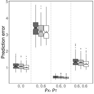
(a) $n=50,p=30$

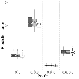
(b) $n=100,p=30$

(c) $n=100,p=100$

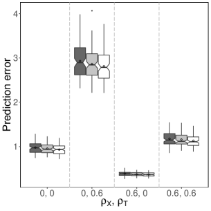
(d) $n=100,p=200$

Figure 6: Boxplots of prediction errors for various simulation settings with $\mbox{SNR}=2$. The layout is the same as in Figure 2 of the main paper.

References

- Aitchison (1982) Aitchison, J. (1982) The statistical analysis of compositional data. Journal of the Royal Statistical Society: Series B, 44, 139–177.
- Aitchison (2003) Aitchison, J. (2003) The Statistical Analysis of Compositional Data. New Jersey, US: Blackburn Press.
- Aitchison and Bacon-Shone (1984) Aitchison, J. and Bacon-Shone, J. (1984) Log-contrast models for experiments with mixtures. Biometrika, 71, 323–330.
- Aitchison and J. Egozcue (2005) Aitchison, J. and J. Egozcue, J. (2005) Compositional data analysis: Where are we and where should we be heading? Mathematical Geology, 37, 829–850.
- Bomar et al. (2011) Bomar, L., Maltz, M., Colston, S. and Graf, J. (2011) Directed culturing of microorganisms using metatranscriptomics. 2, e00012–00011.
- Boulangé et al. (2016) Boulangé, C. L., Neves, A. L., Chilloux, J., Nicholson, J. K. and Dumas, M.-E. (2016) Impact of the gut microbiota on inflammation, obesity, and metabolic disease. Genome Medicine, 8, 42.
- Boyd et al. (2011) Boyd, S., Parikh, N., Chu, E., Peleato, B. and Eckstein, J. (2011) Distributed Optimization and Statistical Learning via the Alternating Direction Method of Multipliers, vol. 3.
- Clarke et al. (2012) Clarke, S. F., Murphy, E. F., Nilaweera, K., Ross, P. R., Shanahan, F., O’Toole, P. W. and Cotter, P. D. (2012) The gut microbiota and its relationship to diet and obesity: New insights. Gut Microbes, 3, 186–202.
- Cong et al. (2017) Cong, X., Judge, M., Xu, W. and Diallo, A. (2017) Influence of feeding type on gut microbiome development in hospitalized preterm infants. Nursing Research, 66, 123–133.
- Cong et al. (2016) Cong, X., Xu, W., Janton, S., Henderson, W. A., Matson, A., McGrath, J. M., Maas, K. and Graf, J. (2016) Gut microbiome developmental patterns in early life of preterm infants: Impacts of feeding and gender. PLOS ONE, 11, 1–19.
- Dinan and Cryan (2012) Dinan, T. and Cryan, J. (2012) Regulation of the stress response by the gut microbiota: implications for psychoneuroendocrinology. Psychoneuroendocrinology, 37, 1369–1378.
- Fan and Tang (2013) Fan, Y. and Tang, C. Y. (2013) Tuning parameter selection in high dimensional penalized likelihood. Journal of the Royal Statistical Society: Series B, 75, 531–552.
- Fanaroff et al. (2003) Fanaroff, A., Hack, M. and MC, W. (2003) The nichd neonatal research network: changes in practice and outcomes during the first 15 years. Seminars in Perinatology, 27, 281–287.
- Feldman and Eidelman (2003) Feldman, R. and Eidelman, A. I. (2003) Direct and indirect effects of breast milk on the neurobehavioral and cognitive development of premature infants. Developmental Psychobiology, 43, 109–119.
- Franz et al. (2011) Franz, C. M., Huch, M., Abriouel, H., Holzapfel, W. H. and Gálvez, A. V. (2011) Enterococci as probiotics and their implications in food safety. International journal of food microbiology, 151 2, 125–40.
- Haltalin (1967) Haltalin, K. C. (1967) Neonatal Shigellosis: Report of 16 Cases and Review of the Literature. JAMA Pediatrics, 114, 603–611.
- Huang et al. (2012) Huang, J., Breheny, P. and Ma, S. (2012) A selective review of group selection in high dimensional models. Statist. Sci., 27, 481–499.
- Li (2015) Li, H. (2015) Microbiome, metagenomics, and high-dimensional compositional data analysis. Annual Review of Statistics and Its Application, 2, 73–94.
- Lin et al. (2014) Lin, W., Shi, P., Feng, R. and Li, H. (2014) Variable selection in regression with compositional covariates. Biometrika, 101, 785–797.
- Lounici et al. (2011) Lounici, K., Pontil, M., van de Geer, S. and Tsybakov, A. B. (2011) Oracle inequalities and optimal inference under group sparsity. Ann. Statist., 39, 2164–2204.
- Morris (2015) Morris, J. S. (2015) Functional regression. Annual Review of Statistics and Its Application, 2, 321–359.
- Mwaniki et al. (2012) Mwaniki, M., Atieno, M., Lawn, J. and Newton, C. (2012) Long-term neurodevelopmental outcomes after intrauterine and neonatal insults: a systematic review. Lancet, 379, 445–452.
- Neu and Rushing (2011) Neu, J. and Rushing, J. M. (2011) Cesarean versus vaginal delivery: long-term infant outcomes and the hygiene hypothesis. Clinics in perinatology, 38 2, 321–31.
- Ramsay and Silverman (2005) Ramsay, J. O. and Silverman, B. W. (2005) Functional Data Analysis. Springer Series in Statistics. Springer, 2nd edn.
- Shi et al. (2016) Shi, P., Zhang, A. and Li, H. (2016) Regression analysis for microbiome compositional data. Ann. Appl. Stat., 10, 1019–1040.
- Stoll et al. (2010) Stoll, B., Hansen, N. and Bell, E. (2010) Neonatal outcomes of extremely preterm infants from the nichd neonatal research network. 126, 443–456.
- Stone (1974) Stone, M. (1974) Cross-validation and multinomial prediction. Biometrika, 61, 509–515.
- Tibshirani (1996) Tibshirani, R. J. (1996) Regression shrinkage and selection via the lasso. Journal of the Royal Statistical Society: Series B, 58, 267–288.
- Tsybakov (2008) Tsybakov, A. B. (2008) Introduction to Nonparametric Estimation. Springer Publishing Company, Incorporated, 1st edn.
- Wei and Huang (2010) Wei, F. and Huang, J. (2010) Consistent group selection in high-dimensional linear regression. Bernoulli, 16, 1369–1384.
- Yuan and Lin (2006) Yuan, M. and Lin, Y. (2006) Model selection and estimation in regression with grouped variables. Journal of the Royal Statistical Society: Series B, 68, 49–67.