iPTF16abc and the population of Type Ia supernovae: Comparing the photospheric, transitional and nebular phases

Abstract

Key information about the progenitor system and the explosion mechanism of Type Ia supernovae (SNe Ia) can be obtained from early observations, within a few days from explosion. iPTF16abc was discovered as a young SN Ia with excellent early time data. Here, we present photometry and spectroscopy of the SN in the nebular phase. A comparison of the early time data with a sample of SNe Ia shows distinct features, differing from normal SNe Ia at early phases but similar to normal SNe Ia at a few weeks after maximum light (i.e. the transitional phase) and well into the nebular phase. The transparency timescales ($t_{0}$) for this sample of SNe Ia range between $\sim$ 25 and 41 days indicating a diversity in the ejecta masses. $t_{0}$ also weakly correlates with the peak bolometric luminosity, consistent with the interpretation that SNe with higher ejecta masses would produce more $\rm{}^{56}Ni$ . Comparing the $t_{0}$ and the maximum luminosity, $\mathrm{L_{max}}$  distribution of a sample of SNe Ia to predictions from a wide range of explosion models we find an indication that the sub-Chandrasekhar mass models span the range of observed values. However, the bright end of the distribution can be better explained by Chandrasekhar mass delayed detonation models, hinting at multiple progenitor channels to explain the observed bolometric properties of SNe Ia. iPTF16abc appears to be consistent with the predictions from the $M_{\rm ch}$ models.

1 Introduction

Type Ia supernovae (SNe Ia) have long been linked to the explosion of a C/O white dwarf (WD) in a binary system (Hoyle & Fowler, 1960), which has been confirmed by observed limits on the progenitor (Nugent et al., 2011; Bloom et al., 2012). However, there is still heated debate about the fundamental physical properties of the system, e.g. the mass of the progenitor, the nature of the companion and the mechanism of the explosion (see, Hillebrandt et al., 2013; Maoz, Mannucci, & Nelemans, 2014, for a review). Many attempts to answer these open questions regarding the physics of SNe Ia have concentrated on observations near maximum light. These observations have been critical to derive global parameters for SNe Ia, e.g. synthesized $\rm{}^{56}Ni$   mass, total ejecta mass (Stritzinger et al., 2006; Scalzo et al., 2014; Dhawan et al., 2016, 2017). However, there is a wealth of information available in observations shortly after explosion as well as at late times ($\sim$ a year after maximum, i.e. the nebular phase, e.g. Maguire et al., 2016; Graham et al., 2017). Early time observations can shed light on the interaction between the SN ejecta and its companion (Kasen, 2010), and can be used to constrain the size of the companion. The signature of such an interaction can be seen as a sharp excess in the UV and blue flux at early epochs (e.g. Cao et al., 2015), however, these pulses can be interpreted differently as in Kromer et al. (2016) and Noebauer et al. (2017). Very early time observations of SNe Ia (Zheng et al., 2013, 2014; Goobar et al., 2014, 2015; Marion et al., 2016; Hosseinzadeh et al., 2017; Miller et al., 2018; Jiang et al., 2017) have shown a diversity in their behaviour shortly after explosion and are a rich source of information regarding the progenitor system and the explosion mechanism.

iPTF16abc was discovered shortly after explosion and showed some interesting early time features. It has a linear rise for the first three days after the time of first light, blue colours at early times compared to normal SNe (e.g. SN 2011fe Nugent et al., 2011), strong carbon features in early spectra that disappear after $\sim$ 7 days (Miller et al., 2018) and the near absence of the Si II  6355 Å  in the earliest spectrum. Here, we present a nebular spectrum of iPTF16abc and analyse the photospheric (i.e. pre-maximum), transitional (i.e. $\sim$ +30 to +100 days) and nebular ($\sim$ +300 days) phase properties of iPTF16abc in context of SNe in the literature.

The observations of the early, photospheric phase mostly probe the outer layers of the ejecta, the late phase, when the $\gamma$-ray escape fraction increases (Jeffery, 1999; Stritzinger et al., 2006), is sensitive to the inner layers of the SN ejecta, which are dominated by iron group elements (IGEs). We, therefore, aim to answer if the features seen in the early phase also manifest at late epochs and hence, whether they are a result of only the composition of the outer layers of the ejecta or also due to the inner core.

The structure of the paper is as follows. We present the dataset in Section 2. We compare the properties of iPTF16abc to a sample of SNe in Section 3. We discuss our results in Section 4 and conclude in Section 5.

2 Data

The intermediate Palomar Transient Factory (iPTF) reported the discovery of iPTF16abc (IAU name: SN2016bln), located 170^′′ from the galaxy NGC 5221 at a redshift of $z=0.023$ and R.A., Dec = 13:34:45.492 +13:51:14.30 (J2000). The line-of-sight that has low Milky Way reddening with $E(B-V)_{MW}=0.028$ mag (Schlafly & Finkbeiner, 2011). The supernova was discovered on 4.4 April 2016 and the first detection was on 3.4 April 2016, the last non-detection was on 2.4 April 2016 (see, Ferretti et al., 2017, for details). The distance to the host galaxy was calculated using a value of $H_{0}$ = 70 kms^-1Mpc^-1 and standard cosmology (i.e. flat, $\Omega_{m}=0.3$) which corresponds to a distance of 100.24 $\pm$ 4.3 Mpc (using a peculiar velocity error on the redshift of 300 kms^-1), or a distance modulus of 35.00 $\pm$ 0.10 mag. Note that since the SN is in the linear part of the Hubble diagram ($z=0.023$), the effect of the assumed cosmology, apart from $H_{0}$ is very small.

As part of a late phase follow-up of iPTF16abc, we obtained a spectrum with the Low Resolution Imaging Spectrometer (LRIS) on the Keck telescope at +342.4 days. The spectrum was obtained as part of program C299 (PI: Kulkarni). It was reduced using the standard LRIS reduction pipeline, lpipe, written in IDL. A summary of the spectra is provided in Table 1. Moreover, we also present photometry at similar epochs with DECam as part of the Dark Energy Camera Legacy Survey (DECaLS), reduced using standard PSF fitting photometry routines in python.

In this study, we also analyse the data presented in Miller et al. (2018) and Ferretti et al. (2017). To this data, we add multi-band data for a sample of SNe Ia from the literature. Since we analyse the multi-band and bolometric properties of a number of SNe Ia, we require coverage from $u\rightarrow H$. We use data from the Carnegie Supernova Project (CSP; Contreras et al., 2010; Stritzinger et al., 2011) and the CfA supernova program (Friedman et al., 2015).

Table 1: Log of spectroscopic observations.

Date	Phase (d)	Telescope + Instrument	Range (Å)	Reference
2016-04-05	$-$15.3	Gemini-North+GMOS	3800 - 9200	M18
2016-04-10	$-$10.9	Keck-I+LRIS	3055 - 10411	M18
2016-04-13	$-$7.8	LCO-2m+FLOYDS	3300 - 9998	M18
2016-04-25	+3.7	LCO-2m+FLOYDS	3300 - 9999	M18
2016-04-30	+8.5	LCO-2m+FLOYDS	3301 - 9999	M18
2016-05-21	+29.2	LCO-2m+FLOYDS	4000 - 8998	M18
2016-06-03	+41.9	LCO-2m+FLOYDS	4000 - 8998	M18
2016-06-11	+49.7	LCO-2m+FLOYDS	4001 - 8999	M18
2016-06-23	+61.4	LCO-2m+FLOYDS	4800 - 9300	M18
2017-03-29	+342.4	Keck-I+LRIS	3200 - 10000	This work

Table 2: This table contains the estimates for the decline rate in the $B$-band, $\Delta m_{15}$, host galaxy extinction, $E(B-V)_{host}$, and the total to selective absorption, $R_{V}$, for the host galaxy of the SN. The $\Delta m_{15}(B)$ is calculated with a Gaussian Process (GP) fit to the observed $B$-band data and the $E(B-V)_{host}$ and $R_{V}$ are calculated from SNooPy fits (Burns et al., 2011) to multi-band data.

SN	$\Delta m_{15}(B)$	$E(B-V)_{host}$	$\sigma$	$R_{V}$
	(mag)	(mag)	(mag)
SN2004eo	1.42	0.128	0.024	0.9
SN2004ey	0.96	0.019	0.020	3.1
SN2005el	1.35	0.015	0.012	3.5
SN2005ke	1.78	0.263	0.033	0.8
SN2005ki	1.28	0.016	0.013	3.4
SN2005M	0.90	0.060	0.021	3.4
SN2006ax	1.00	0.016	0.015	2.9
SN2006D	1.43	0.134	0.025	2.5
SN2006et	0.90	0.254	0.025	1.9
SN2006kf	1.63	0.032	0.011	4.1
SN2006mr	1.83	0.089	0.039	2.9
SN2007af	1.17	0.178	0.024	2.1
SN2007ax	1.90	0.213	0.049	2.6
SN2007bc	1.59	0.207	0.025	1.8
SN2007bd	1.10	0.058	0.022	2.1
SN2007le	0.97	0.388	0.023	1.7
SN2007on	1.88	0.000	0.000	3.5
SN2007S	0.77	0.478	0.026	1.9
SN2008bc	0.85	0.000	0.000	3.1
SN2008hv	1.25	0.074	0.023	2.1
SN2008ia	1.29	0.066	0.016	3.8
iPTF16abc	0.91	0.070	0.016	3.1

Table 3: Distances for the SNe in our sample. These were used to calculate the absolute (pseudo)-bolometric flux.

SN	$\mu$	$\sigma$
	(mag)	(mag)
SN2004eo	34.03	0.14
SN2004ey	34.01	0.15
SN2005el	34.05	0.14
SN2005ke	31.84	0.08
SN2005ki	34.74	0.11
SN2005M	35.0	0.09
SN2006ax	34.46	0.12
SN2006D	33.1	0.22
SN2006et	34.82	0.10
SN2006kf	34.78	0.10
SN2006mr	31.15	0.23
SN2006X	32.17	0.32
SN2007af	32.16	0.32
SN2007ax	32.2	0.27
SN2007bc	34.89	0.10
SN2007bd	35.73	0.07
SN2007le	31.88	0.36
SN2007on	31.45	0.08
SN2007S	34.07	0.14
SN2008bc	34.17	0.14
SN2008fp	32.16	0.32
SN2008hv	33.85	0.16
SN2008ia	34.97	0.10
iPTF16abc	35.01	0.09

3 Results

3.1 Spectroscopy

Figure 1 shows observed spectra of iPTF16abc from $-$15.3 days to +8.5 d relative to $B-$band maximum and figure 2 from +29.2 d to +342.4 d, compared to those of some normal SNe Ia at similar epochs ($\pm$2.5 d). Specifically, the comparison sample comprises spectra for the well-studied and nearby SN 2011fe (Nugent et al., 2011; Pereira et al., 2013; Maguire et al., 2014; Mazzali et al., 2014; Taubenberger et al., 2015) together with those for normal SNe Ia in the CSP sample of Table 2 that are characterised by $E(B-V)<$0.2 mag and no high-velocity features (i.e. SN2004ey, SN2005el, SN2005na, SN2006ax and SN2008hv, Folatelli et al. 2013). We also plot the available spectra for the overluminous SN 1991T (Filippenko et al., 1992; Phillips et al., 1992; Ruiz-Lapuente et al., 1992; Gómez & López, 1998; Silverman, Ganeshalingam, & Filippenko, 2013) and SN 1999aa (Garavini et al., 2004; Matheson et al., 2008; Silverman, Ganeshalingam, & Filippenko, 2013) in figures 1 and 2.

Spectra of iPTF16abc before maximum show distinct peculiarities compared to the bulk of normal SNe Ia at these early epochs (Miller et al., 2018). The most striking difference is found across the Si ii $\lambda 6355$ and Ca ii near-IR triplet features around 6000 and 8000 Å, respectively. Both these features are usually strong in pre-maximum spectra of normal SNe Ia, while they are much weaker in iPTF16abc. A SNID classification of the -11 d spectrum in Figure 1 points to a best match with SN 1999aa, an overluminous, peculiar SN Ia (Garavini et al., 2004), which is consistent with the deep Ca H&K feature in iPTF16abc that is not seen in SN 1991T (Figure 1). The early time ($<$ -10 days) colours for iPTF16abc are significantly bluer (see Miller et al., 2018) and the colour evolution is significantly flatter than other overluminous SNe with such early observations (e.g. SN2012fr; Contreras et al., 2018). We emphasize, however, that our results are independent of the classification of iPTF16abc as a 91T-like, 99aa-like or normal SN Ia. As we will discuss in Section 4, this behaviour is consistent with the suggestion from Miller et al. (2018) that strong mixing could have occurred in the ejecta of iPTF16abc.

Despite the pronounced differences seen at early-epochs, the spectral time evolution of iPTF16abc from peak brightness to about a year after is remarkably similar to the one observed in normal SNe Ia which have been shown to be similar to 91T-like/99aa-like SNe (Filippenko et al., 1992; Garavini et al., 2004), also consistent with the SNID classification from the post maximum spectrum, presented in Miller et al. (2018). Good agreements with the comparison spectra are found at all epochs both in terms of colours (see also Miller et al., 2018) and velocities/ strength of individual features. The similarities between iPTF16abc and the comparison sample extend up to transitional and nebular phases ($\gtrsim$ 30 d), when the inner regions of the SN ejecta are probed.

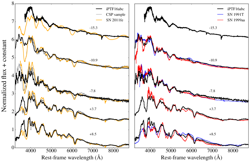
Figure 1: Left: The early time ($<$ +10 days) spectral time sequence of iPTF16abc (black) is compared to the spectra of SN 2011fe (orange), some normal SNe Ia in the CSP sample of Table 2 (grey) Right: The spectral time sequence is compared to SN 1991T and SN 1999aa at similar epochs ($\pm$2.5 d). Spectra in the left panel are normalized by their values at $\sim$ 5200 Å, the top four in the right panel by their values at $\sim$ 5500 Å and the last spectra by their values at $\sim$ 5200 Å.

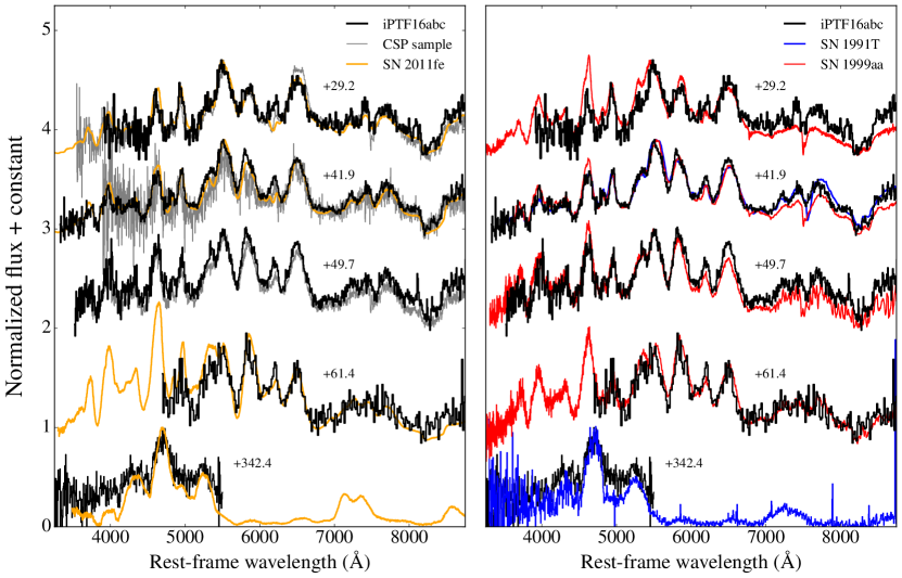
Figure 2: Same as Figure 1 but for the transitional and the nebular phase. The top four spectra in the right panel are normalised to their values at $\sim$ 5500 Å and the last spectrum by its value at $\sim$ 4700 Å.

3.1.1 Nebular Phase

Connections between SN Ia properties at early times and those at epochs $\gtrsim$ 150 d have been proposed, including correlations between the strength of the Fe $\lambda$4700 feature and $\Delta m_{15,B}$ (Mazzali et al., 1998, but see also Blondin et al. 2012) and between nebular line velocities and colours at peak (Maeda et al., 2011). Measuring late-time properties of iPTF16abc can improve our understanding of the observed peculiarities at early times. We obtained a spectrum of iPTF16abc at +342.4 days close to a year after maximum light. In Figure 2 we qualitatively compare the spectrum to SN 2011fe, SN 1991T and SN 1999aa in the nebular phase and find no striking differences.

We measured the full width at half maximum of the iron feature at $\sim$ 4700Å  to be 17 510 $\pm$ 891 km s^-1. Mazzali et al. (1998) found a relation between the FWHM of this feature and $\Delta m_{15}(B)$, although with a large sample of SNe Blondin et al. (2012) find no strong relation. In Figure 3, we plot the FWHM of the 4700Å  feature for iPTF16abc with the sample of SNe from Blondin et al. (2012) and find that it is towards the higher end of the distribution of line widths but is consistent with the rest of the SNe in the literature.

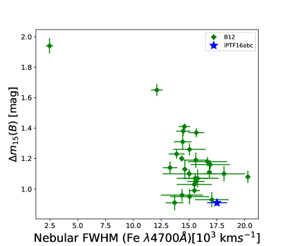
Figure 3: The $\Delta m_{15}(B)$ for the supernovae from the CfA SN program (Blondin et al., 2012) is plotted against the full width at half maximum (FWHM) of the Fe $\lambda$ 4700 Å  feature (green diamonds). iPTF16abc is plotted as the blue star and appears to be consistent with the distribution for the CfA sample.

Table 4: The near infrared second maximum timing for iPTF16abc.

Filter	$t_{2}$
	(d)
Y	34.4 $\pm$ 1.23
J	34.2 $\pm$ 1.23
H	33.2 $\pm$ 1.4

3.2 Bolometric properties

Bolometric properties of SNe Ia have been demonstrated to hold important information regarding the underlying physical parameters of the progenitors, e.g. $M_{\rm ej}$   , $\rm{}^{56}Ni$   mass (Contardo, Leibundgut, & Vacca, 2000; Stritzinger et al., 2006; Scalzo et al., 2014). We compute the bolometric light curves for SNe with photometry from $u$ to $H$ filters. The observed magnitudes are dereddened using the reddening law in Cardelli, Clayton & Mathis (1989). Specifically, $E(B-V)$ and $R_{V}$ values are computed using SNooPy with the colour-stretch parameter (Burns et al., 2011, 2014) and are summarized in Table 2. Filter gaps and overlaps are treated as in Dhawan et al. (2016, 2017) and the apparent flux is converted to absolute fluxes using distances in Table 3. We use a cubic spline interpolation to derive the values of the maximum luminosity, $\mathrm{L_{max}}$, from the bolometric light curves. Here we compare the early and late time bolometric properties of a sample of Type Ia supernovae with the inferred values for iPTF16abc. Since the light curve shape for SNe Ia can depend on the host galaxy reddening for highly-reddened SNe (Leibundgut, 1988; Amanullah & Goobar, 2011; Bulla et al., 2018), we only use SNe with $E(B-V)<0.5$ mag. ⁵⁶Ni mass ($\rm M_{{}^{56}Ni}$) values are derived from $\mathrm{L_{max}}$ using Arnett’s rule, i.e. assuming that the instantaneous rate of energy deposition equals the output flux at maximum (Arnett, 1982):

Table 5: The derived $\rm M_{{}^{56}Ni}$  for the sample of SNe with a measured $t_{0}$ under two different assumptions on the rise time of the SNe. From the values below we find that the inferred $\rm M_{{}^{56}Ni}$  is within the errors even with individual rise times for each SN.

SN	Lmax	$\sigma$	M${}_{\mathrm{{}^{56}Ni}}$ (fixed rise)	$\sigma$	M${}_{\mathrm{{}^{56}Ni}}$ (variable rise)	$\sigma$
	1043 erg/s	1043 erg/s	M⊙	M⊙	M⊙	M⊙
SN2004eo	1.08	0.14	0.54	0.11	0.44	0.08
SN2004ey	1.27	0.21	0.63	0.14	0.59	0.12
SN2005el	1.20	0.18	0.6	0.13	0.50	0.10
SN2005ke	0.31	0.04	0.15	0.03	0.11	0.02
SN2005ki	1.19	0.37	0.6	0.21	0.51	0.17
SN2005M	1.33	0.36	0.67	0.21	0.63	0.18
SN2006ax	1.51	0.38	0.75	0.22	0.69	0.19
SN2006D	1.35	0.32	0.68	0.19	0.55	0.15
SN2006et	1.60	0.32	0.80	0.20	0.76	0.17
SN2006kf	0.97	0.09	0.48	0.08	0.37	0.06
SN2006mr	0.12	0.05	0.06	0.03	0.04	0.02
SN2007af	1.51	0.43	0.75	0.24	0.66	0.20
SN2007ax	0.17	0.05	0.08	0.03	0.06	0.02
SN2007bc	1.47	0.29	0.73	0.18	0.57	0.13
SN2007bd	1.31	0.31	0.66	0.18	0.59	0.15
SN2007le	0.91	0.28	0.45	0.16	0.42	0.14
SN2007on	0.58	0.03	0.29	0.05	0.21	0.03
SN2007S	1.73	0.35	0.86	0.22	0.84	0.19
SN2008bc	1.37	0.12	0.68	0.12	0.65	0.09
SN2008hv	1.22	0.30	0.61	0.18	0.52	0.14
SN2008ia	1.32	0.14	0.66	0.12	0.56	0.09
iPTF16abc	1.22	0.20	0.61	0.14	0.55	0.11

$$\epsilon_{Ni}(t_{R},1~{}M_{\odot})=\\ \alpha\cdot(6.45\cdot 10^{43}e^{-t_{R}/8.8}+1.45\cdot 10^{43}e^{-t_{R}/111.3})\,{\rm erg\,s^{-1}},$$ (1)

where $t_{R}$ is the bolometric rise time and $\alpha$ is the parameter that accounts for deviations from Arnett’s rule. These departures from $\alpha=1$ could be due to the ⁵⁶Ni distribution, however, detailed model calculations of SNe Ia find that $\alpha=1$ with a scatter of 10-15$\%$ (Blondin et al., 2013; Blondin et al., 2017). The impact of this on further parameter estimation is discussed below. Assuming Arnett’s rule is obeyed and a rise time of $t_{R}=$19 days with an error of 3 days (Stritzinger et al., 2006; Dhawan et al., 2016), we can derive a $\rm M_{{}^{56}Ni}$  from the computed value of $\mathrm{L_{max}}$:

$$\frac{\mathrm{M_{{}^{56}Ni}}}{\mathrm{M_{\odot}}}=\frac{L_{max}}{2.0(\pm 0.3)\times 10^{43}\mathrm{erg\,s^{-1}}}~{}~{}.$$ (2)

For iPTF16abc (see Table 5), the small difference in the inferred $\rm M_{{}^{56}Ni}$  from Miller et al. (2018) is due to the different methods adopted for calculating the distances. We discuss the impact of the rise time in Section 4.1. We note that some SNe in our sample have also been studied in detail in the literature (e.g., SN2007on; Ashall et al., 2018). We find our inferred $\rm{}^{56}Ni$   mass in good agreement with the values they report.

Table 6: The values of the transparency timescales for a sample of SNe from the literature with sufficient data. The first estimate assume a rise time of 19 d whereas the second assumes a rise time that varies as a function of the measured $\Delta m_{15}(B)$. An additional systematic uncertainty of $\sim$ 2 days should be added in quadrature to the error on $t_{0}$ due to the uncertainty in knowing the rise time. The values from the two different estimates are comparable within the systematic errors.

SN	$t_{0}$ (fix rise)	err	$t_{0}$ (variable rise)	err
	(days)	(days)	(days)	(days)
SN2004eo	35.34	0.06	36.67	0.08
SN2004ey	34.64	0.03	34.90	0.03
SN2005el	28.38	0.03	29.49	0.05
SN2005ke	28.87	0.02	31.35	0.05
SN2005ki	29.85	0.04	30.69	0.06
SN2005M	38.01	0.14	38.22	0.14
SN2006ax	35.51	0.08	35.83	0.07
SN2006D	28.47	0.02	29.89	0.05
SN2006et	38.18	0.09	38.39	0.09
SN2006kf	27.62	0.04	28.90	0.06
SN2006mr	24.54	0.01	26.21	0.02
SN2007af	33.50	0.06	34.42	0.08
SN2007ax	26.12	0.02	27.84	0.04
SN2007bc	27.28	0.05	28.74	0.05
SN2007bd	31.21	0.01	31.59	0.01
SN2007le	37.12	0.07	37.57	0.08
SN2007on	26.63	0.01	29.08	0.06
SN2007S	40.18	0.09	40.16	0.09
SN2008bc	36.60	0.05	36.75	0.05
SN2008hv	29.88	0.04	30.87	0.07
SN2008ia	28.42	0.22	29.11	0.24
iPTF16abc	39.50	0.21	39.76	0.22

We also calculate the transparency timescale ($t_{0}$) for the sample of SNe, defined by Jeffery (1999) as a parameter that governs the time-varying $\gamma$-ray optical depth behaviour of a supernova. We determined $t_{0}$ by fitting the radioactive decay energy deposition to the late time (forty to ninety days) bolometric light curve:

$$E_{{\rm dep}}=E_{{\rm Ni}}+E_{{\rm Co~{}e^{+}}}+[1-{\rm exp(-\tau_{\gamma})}]E_{{\rm Co~{}\gamma}}\\[5.69054pt] =\lambda_{{\rm Ni}}{{\rm N_{Ni0}}}~{}{\rm exp(-\lambda_{{\rm Ni}}t)Q_{{\rm Ni~{}\gamma}}}\\[5.69054pt] +\lambda_{{\rm Co}}{\rm N_{Ni0}}{\frac{\lambda_{{\rm Ni}}}{\lambda_{{\rm Ni}}-\lambda_{{\rm Co}}}}[{\rm exp(-\lambda_{{\rm Co}}t)-exp(-\lambda_{{\rm Ni}}t)}]\\[5.69054pt] \times\{Q_{\rm Co~{}e^{+}}+Q_{{\rm Co~{}\gamma}}[1-{\rm exp(-\tau_{\gamma})}]\},$$ (3)

where the factor (1-exp(-$\tau_{\gamma}$)) is replaced by 1 for ⁵⁶Ni since complete trapping of $\gamma$-rays occurs at early times, when most of the light curve is powered by ⁵⁶Ni. where $\lambda_{Ni}$ and $\lambda_{Co}$ are the e-folding decay times of 8.8 days and 111.3 days for $\rm{}^{56}Ni$   and $\rm{}^{56}Co$   respectively. $Q_{\mathrm{Ni}\,\gamma}$ (1.75 MeV) is the energy release per $\rm{}^{56}Ni$   $\rightarrow$ $\rm{}^{56}Co$   decay. $Q_{\mathrm{Co}\,\gamma}$ (3.61 MeV) and $Q_{\mathrm{Co}\,e^{+}}$ (0.12 MeV) are the $\gamma$-ray and positron energies, respectively, released per $\rm{}^{56}Co$   $\rightarrow$ $\rm{}^{56}Fe$   decay (see Stritzinger et al., 2006). Equation 3 is only applicable in the optically thin limit, when the thermalized photons can freely escape.

$\tau_{\gamma}$ is the mean optical depth, calculated by integrating from the point of emission to the surface of the ejecta (see Jeffery, 1999, for a derivation of the expression). It has a simple t^-2 dependence, given as,

$$\tau_{\gamma}=\frac{t_{0}^{2}}{t^{2}}.$$ (4)

where $t_{0}$ is the transparency timescale, which by construction in Jeffery (1999) is the epoch at which the optical depth is unity.

The value of the transparency timescale can be directly related to the total ejecta mass ($M_{\rm ej}$ ) with the following equation (Jeffery, 1999; Stritzinger et al., 2006; Dhawan et al., 2017)

$$M_{\rm ej}=1.38\cdot\left(\frac{1/3}{q}\right)\cdot\left(\frac{v_{e}}{3000\,\mathrm{kms^{-1}}}\right)^{2}\cdot\left(\frac{t_{0}}{36.80\,days}\right)^{2}\mathrm{M_{\odot}}.$$ (5)

Equation 5 encapsulates the capture rate of $\gamma$-rays in an expanding spherical volume for a given distribution of the radioactive source. We discuss the typical parameter values for canonical SN Ia models to map $t_{0}$ to $M_{\rm ej}$ , however, we note that we do not use any calculations for $M_{\rm ej}$ in our analysis and only use the observed $t_{0}$ values. $q$ is a qualitative description of the distribution of the material within the ejecta, with one third being a uniform distribution and higher values reflecting more centrally-concentrated $\rm{}^{56}Ni$ ( more typical of subluminous 1991bg-like SNe (Mazzali, et al., 1997)). The e-folding velocity $v_{e}$ provides the scaling length for the expansion, which is $\sim$ 3000 km $s^{-1}$ for Chandrasekhar-mass ($M_{\rm ch}$) explosions corresponding to typical brightness SNe Ia and on average slightly lower for sub-$M_{\rm ch}$ WDs. For both $M_{\rm ch}$ and sub-$M_{\rm ch}$ models it ranges between $\sim$ 2700 - 3200 km $s^{-1}$. For an ejecta with Y_e = 0.5, which is appropriate for SNe Ia, the $\gamma$-ray opacity is a constant of 0.025 cm² g^-1 (Swartz, Sutherland, & Harkness, 1995). Given the range of possible values for $q$ and $v_{e}$, we do not proceed to infer M_ej for the SNe in our sample.

Because the UVOIR light curve is not truly bolometric, there is an implicit assumption that the flux redward of the $H$ band and bluewards of the $u$ band have very small contributions to the bolometric light curve. This assumption is supported by modelling that shows that the infrared catastrophe does not occur until $\sim$ 1 year post explosion or later, whereas typical values of $t_{0}$ are between 20 and 50 days and the line-blanketing opacity in the UV remains high (Blondin, Dessart, & Hillier, 2015; Fransson & Jerkstrand, 2015).

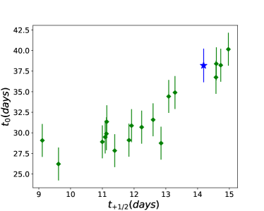
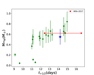
Figure 4: (Left): $t_{0}$ is plotted against $t_{+1/2}$ for the sample of objects with sufficient late time data to measure $t_{0}$. There is a strong correlation between the two parameters, with $r\sim 0.85$. iPTF16abc is shown as the blue star and is consistent with the relation. (Right) $\rm M_{{}^{56}Ni}$  is plotted against $t_{+1/2}$, the red points are predictions from the models of Wilk, Hillier, & Dessart (2017) for sub-M_Ch, M_Ch and super-M_Ch progenitors.

Recent studies of the diagnostics of ejecta mass (e.g. Wilk, Hillier, & Dessart, 2017) compute the $t_{+1/2}$ for different ejecta mass models. $t_{+1/2}$ is defined as the time the bolometric light curve takes to decline to half of its peak luminosity (Contardo, Leibundgut, & Vacca, 2000). In Figure 4 we plot the $t_{+1/2}$ against $t_{0}$ for the sample with sufficient data. Unsurprisingly, we find a strong correlation ($r\sim 0.85$) for the objects in our sample, suggesting that the SNe that take longer to decline to half the peak luminosity also have optically thick ejecta for longer. Since Jeffery (1999) suggest that $t_{0}$ is directly related to $M_{\rm ej}$ and this equation has been used to calculate $M_{\rm ej}$ for SNe Ia (Stritzinger et al., 2006; Scalzo et al., 2014), this implies that $t_{+1/2}$ can also be used as a diagnostic for the ejecta mass.

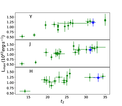
Figure 5: The (pseudo-) bolometric peak luminosity is plotted against the timing of the second maximum in the $YJH$ filters. For both parameters, in this figure, the rise time is assumed to be 19 days. The blue star is iPTF16abc. It lies on the relation for all other SNe Ia, though towards the brighter side.

3.3 Near Infrared light curves

The near infrared morphology of SN Ia light curves has been shown to be markedly different from the optical (Elias et al., 1981, 1985). The SNe show a characteristic second peak in the $izYJHK$ filters (Mandel et al., 2009; Biscardi et al., 2012; Dhawan et al., 2015) and a less pronounced “shoulder”-like feature in the $V$ and $r$ bands. Theoretical studies have shown that these features are caused by a recombination wave in the IGEs in the ejecta from doubly- to singly-ionised (Kasen, 2006; Blondin, Dessart, & Hillier, 2015), hence, the NIR second maximum is an important parameter to test whether the observed peculiarities in iPTF16abc could be arising due to the properties of the central IGE core. iPTF16abc shows a distinct second maximum in the $YJH$ filters, consistent with the theoretical prediction for an SN Ia that produced $\sim$ 0.6 $M_{\odot}$ of $\rm{}^{56}Ni$   (Kasen, 2006).

The values for the timing of the second maximum ($t_{2}$) for iPTF16abc are presented in Table 4 and shown in Figure 5. The $t_{2}$ values of iPTF16abc are consistent within the range for normal SNe Ia (Biscardi et al., 2012; Dhawan et al., 2015), although they are at the higher end like 91T-like/99aa-like SNe. Dhawan et al. (2016) found a correlation between the peak (pseudo-) bolometric luminosity and $t_{2}$ for a sample of SNe with low reddening from the host galaxy dust. As shown in Figure 5, the value for iPTF16abc lies on the expected relation.

Table 7: Nebular Phase photometry with DECam

MJD	Phase (d)	filter	magnitude	$\sigma$
			(mag)	(mag)
57818.30	320.20	desg	22.249	0.053
57818.30	320.20	desr	23.323	0.053
57814.39	316.29	desz	22.501	0.191

3.4 Nebular Phase Photometry

iPTF16abc was also observed at epochs between +316-+320 days by the DECaLS survey in $g,r,z$ filters. The photometry on the DECaLS images is presented in Table 7. The decrease of 6.6 mag from peak to $\sim$ +300 days (see Figure 6) is consistent with the expected value for normal SNe Ia (e.g. Stritzinger & Sollerman, 2007). We also find that the $r$-band absolute magnitude of -11.4 $\pm$ 0.11 mag is within the range of observed values in the literature (Lair et al., 2006) at late phases of $\sim$ 1 year post maximum. This further demonstrates that , at late epochs, the observed properties of iPTF16abc are within the observed distribution for normal SNe Ia. We note that since there is only $r$-band photometry available for SNe Ia at these late epochs (out of the three filters presented here), it is the only one for which we can compare iPTF16abc to literature values for a sample.

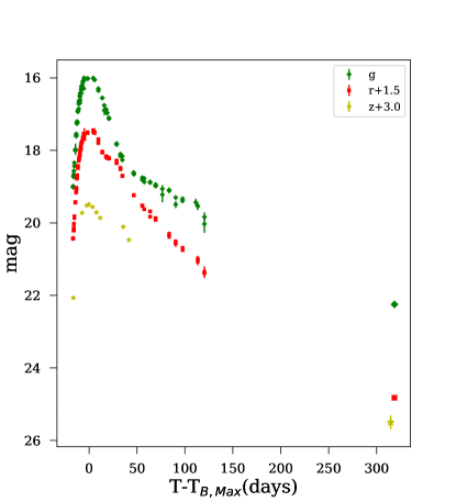
Figure 6: $g$,$r$,$z$ light curves of iPTF16abc from Miller et al. (2018), along with the nebular phase ($>$ + 300 days) data points from the DECaLS survey. The legend gives the magnitude offsets for the $r$ and $z$ light curves.

4 Discussion

The early light curve and spectral evolution of iPTF16abc showed marked peculiarities that were interpreted as a signature of strong outward mixing of $\rm{}^{56}Ni$  and/or interaction with diffuse material (Miller et al., 2018). In the case of strong mixing, the temperature and thus ionisation level of the outer ejecta would be higher compared to the case of a centrally-concentrated distribution of $\rm{}^{56}Ni$  more commonly inferred for normal SNe Ia. This would explain why in iPTF16abc not only C ii features are stronger (Miller et al., 2018) but also Si ii and Ca ii features are weaker compared to what is seen for the bulk of normal SNe Ia. Shallow silicon and calcium features are also observed in peculiar events such as 2002cx-like and 1991T-like SNe Ia. Models for both 2002cx-like (pure deflagration models, e.g. Sahu et al., 2008; Kromer et al., 2013) and 1991T-like (Ruiz-Lapuente et al., 1992; Mazzali et al., 1995; Sasdelli et al., 2014; Fisher & Jumper, 2015; Seitenzahl et al., 2016; Zhang et al., 2016) SNe Ia invoke the presence of $\rm{}^{56}Ni$  and IGEs in the outer ejecta, thus corroborating the idea that mixing might be responsible for the photometric and spectroscopic features seen in iPTF16abc. The nebular spectrum of iPTF16abc, however, looks consistent with the normal SN 2011fe, and the measured line width of the 4700 Å  agrees with the width-decline rate relation for a sample of normal SNe from the literature (Figure 3). The likely source of these peculiarities could therefore arise from the outer layers of the ejecta, and probably not from the central core of IGEs.

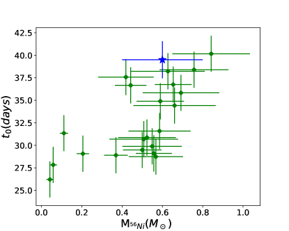
Figure 7: The transparency timescale, $t_{0}$, is plotted against the ⁵⁶Ni mass for a sample of SN Ia with $u\rightarrow H$ band coverage (green diamonds). There is a weak correlation ($r\sim 0.67$) between the two parameters. iPTF16abc is plotted as a blue star and appears to be consistent with the general trend of $t_{0}$ versus $M_{{}^{56}\rm Ni}$.

The transparency timescale is strongly tied to the ejecta mass of the SN (Jeffery, 1999; Stritzinger et al., 2006; Scalzo et al., 2014), therefore, given the uncertainties in driving the ejecta masses from $t_{0}$, we use $t_{0}$ directly for our analysis. As shown in Figure 7, we find that the total $\rm M_{{}^{56}Ni}$  is correlated with the transparency timescale for our sample of SNe Ia such that objects with a longer $t_{0}$ produce more $\rm M_{{}^{56}Ni}$  also indicating a possible positive relation of the ejecta mass with the amount of synthesized $\rm{}^{56}Ni$   in agreement with previous studies (Stritzinger et al., 2006; Scalzo et al., 2014). iPTF16abc is consistent with this relation between $t_{0}$ and $\rm M_{{}^{56}Ni}$. For both parameters, we assume a canonical rise time of 19 days. In Section 4.1, we discuss the impact of this assumption.

Table 8: The values of the (pseudo-) bolometric peak luminosities and the transparency timescales for a sample of SNe from the literature with sufficient data to measure both quantities. An additional systematic uncertainty of $\sim$ 2 days should be added in quadrature to the error on $t_{0}$ due to the uncertainty in knowing the rise time.

SN	t+1/2	$t_{0}$ (variable rise)	err
	(d)	(d)	(d)
SN2004ey	13.29	34.9	0.03
SN2005el	11.09	29.49	0.05
SN2005ke	11.14	31.35	0.05
SN2005ki	12.24	30.69	0.06
SN2005M	14.73	38.22	0.14
SN2006D	11.13	29.89	0.05
SN2006et	14.59	38.39	0.09
SN2006kf	11.00	28.9	0.06
SN2006mr	9.62	26.21	0.02
SN2007af	13.09	34.42	0.08
SN2007ax	11.39	27.84	0.04
SN2007bc	12.85	28.74	0.05
SN2007bd	12.60	31.59	0.01
SN2007on	9.11	29.08	0.06
SN2007S	14.97	40.16	0.09
SN2008bc	14.58	36.75	0.05
SN2008hv	11.92	30.87	0.07
SN2008ia	11.84	29.11	0.24
iPTF16abc	14.14	39.76	0.09

The right panel of Figure 4 shows a weak correlation between the half light time for the bolometric light curve ($t_{+1/2}$) and the $\rm M_{{}^{56}Ni}$  as in Contardo, Leibundgut, & Vacca (2000). Comparing the observed $t_{+1/2}$ from models for three different ejecta masses (Wilk, Hillier, & Dessart, 2017), all producing 0.6 $M_{\odot}$ of $\rm M_{{}^{56}Ni}$ (i.e. the same as the estimate for iPTF16abc Miller et al., 2018) we find that the range of $t_{+1/2}$ observed in SNe Ia is higher, possibly indicating that there is a large range of ejecta masses to explain the observations of the sample of SNe Ia. The observed $t_{+1/2}$ range could indicate that the sample of SNe corresponds to a range of ejecta masses. Since the lowest $M_{\rm ej}$ investigated in Wilk, Hillier, & Dessart (2017) is 1.02 $M_{\odot}$, lower $t_{+1/2}$ could imply smaller ejecta masses for the lower luminosity SNe in the sample (see also Blondin et al., 2017).

4.1 Rise time

In this section we discuss the effect of using different prescriptions for the rise time as an input to calculate the $\rm M_{{}^{56}Ni}$  and $t_{0}$. Although iPTF16abc has early time observations that can strongly constrain the rise ($\sim$ 18 days in the $g$-band, Miller et al., 2018), for a sample of SNe, the early behaviour is not as well-characterised. Our canonical assumption in Section 3 was to use a rise time of 19 days along with an error of 3 days to capture the diversity in the observed values for the population of SNe Ia (e.g. Ganeshalingam, Li, & Filippenko, 2011). In Ganeshalingam, Li, & Filippenko (2011), the authors find that the rise time is correlated with the post-peak decline rate and they derive a linear relation between the $B$-band rise time and $\Delta m_{15,B}$:

$$t_{R,B}=17.5-5\cdot(\Delta m_{15,B}-1.1)$$ (6)

The bolometric maximum occurs on average one day before $B_{max}$ (Contardo, Leibundgut, & Vacca, 2000; Scalzo et al., 2014), hence, we derive the rise time using

$$t_{R,bol}=16.5-5\cdot(\Delta m_{15,B}-1.1)$$ (7)

Hence, faster declining SNe Ia would have a faster rise. From equation 1 we can see that a faster rise time implies a smaller $\rm M_{{}^{56}Ni}$  for the same $\mathrm{L_{max}}$. The error on the rise from this method is $\sim$ 2 days (Scalzo et al., 2014). The impact of the rise time on the inferred $\rm M_{{}^{56}Ni}$  is shown in Table 5. It is clear from the table that even with a varying rise time across the sample, the $\rm M_{{}^{56}Ni}$  estimates are within the errors.

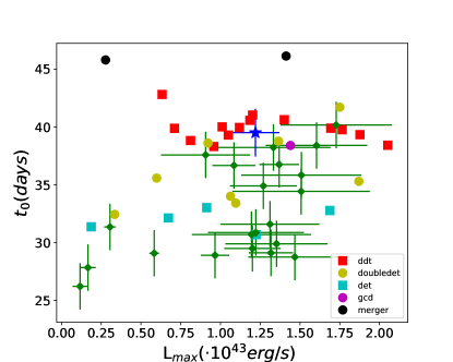
Figure 8: The transparency timescale is plotted against the peak bolometric luminosity for the sample of SNe in this study. Overplotted are the expectations from the different explosion scenarios. The red squares are the three dimensional $M_{\rm ch}$ delayed detonation models of Seitenzahl et al. (2013), the magenta circle is the $M_{\rm ch}$ gravitationally confined detonation of Seitenzahl et al. (2016). The yellow circles are the sub-$M_{\rm ch}$ “double-detonation” models of Fink et al. (2010) whereas the yellow squares are the sub-$M_{\rm ch}$ pure detonations presented in Sim et al. (2010). The two black circles are the violent merger models of Pakmor et al. (2010) and Pakmor et al. (2012).

We note that the estimation of $t_{0}$ from the (pseudo)-bolometric light curve, depends on the inference of the number of $\rm{}^{56}Ni$   atoms, which in turn is sensitive to the $\alpha$ parameter. Since the deviations from the $\alpha=1$ case are of the order 10-15$\%$, the difference in the estimated $t_{0}$ is within the errors.

4.2 Comparison with explosion models

We computed $t_{0}$ and $\rm M_{{}^{56}Ni}$  for a sample of SNe and found that these quantities were weakly correlated (see also Stritzinger et al., 2006; Scalzo et al., 2014). iPTF16abc lies on the $t_{0}$ - $\rm M_{{}^{56}Ni}$  relation for the SNe studied here, suggesting that the amount of $\rm M_{{}^{56}Ni}$  and the progenitor mass for the SNe is compatible with the normal population of SNe Ia. Here, we compare the relation between $t_{0}$ and $\mathrm{L_{max}}$  to predictions from different theoretical models, since we want to directly compare observable quantities from the data to the model predictions. A range of $t_{0}$ values from $\sim$ 25 to 40 days in itself would suggest that not all SNe Ia could arise from the same ejecta mass (Stritzinger et al., 2006; Scalzo et al., 2014).

In Figure 8 we plot the $t_{0}$ against the $\mathrm{L_{max}}$  for the sample of SNe in this study and compare them to the predictions from various explosion scenarios. The synthetic observables were taken from the Heidelberg Supernova Model Archive (HESMA; Kromer, Ohlmann, & Roepke, 2017). We find that the bright end of the distribution appears to be consistent with the $M_{\rm ch}$ delayed detonation models of Seitenzahl et al. (2013). The faint end of the relation is traced well by the sub-$M_{\rm ch}$ models of Fink et al. (2010) and Sim et al. (2010) although some of the predictions from the most massive sub-$M_{\rm ch}$ models seem consistent with the brightest observed SNe too. The violent merger models imply a longer transparency timescale than observed for any SNe in the sample. iPTF16abc is consistent with the observed relation and appears to be closer to the trend for the $M_{\rm ch}$ models. We find our conclusion that sub-$M_{\rm ch}$ scenario are consistent with nearly the entire range of observed $L_{max}$ and $t_{0}$ whereas the $M_{\rm ch}$ can only explain the bright end is supported by recent theoretical studies which find that the entire width-luminosity relation reproducable by sub-Chandra models whereas the Chandrasekhar mass models only reproduce the bright end (Goldstein & Kasen, 2018). This conclusion is also supported by a comparison of observations and model predictions presented in Shen et al. (2017). The two overluminous SNe in our sample with SNID classifications of 91T-like (Folatelli et al., 2013) are both consistent with M_ch model prediction. Fisher & Jumper (2015) suggest that M_ch WD explosions that lack a vigourous deflagration phase would produce 91T-like SNe. Since these explosions would also have higher $\rm{}^{56}Ni$   mixing, this might indicate that overluminous SNe that show 91T-like spectral features have shorter deflagration phases.

We note that iPTF16abc appears to have $t_{0}$ estimates consistent with $M_{\rm ej}=1.4M_{\odot}$, under the assumption that $q\sim 1/3$. This value of $q$ would point towards strong $\rm{}^{56}Ni$   mixing in the ejecta in line with the findings of Miller et al. (2018). Miller et al. (2018) cite a discrepancy between the early time observables and the early colours predicted for the sub-Chandrasekhar “double-detonations” of Noebauer et al. (2017) as a reason that iPTF16abc is likely not a result of the double detonation of a sub-$M_{\rm ch}$ WD. The late-time bolometric properties would point to a similar conclusion.

Using the transparency timescale we can calculate the epoch at which the energy deposition from the $\gamma$ rays is equal to the contribution from the positrons (hereafter, $t_{c}$, see Childress et al., 2015). For iPTF16abc, $t_{c}=205.2\pm 11.3$ days which is consistent with the calculated value for the $M_{\rm ch}$ delayed detonation model (DDC10) of Blondin et al. (2013) of $t_{c}\sim 214$  days, compared to values between 160 and 180 days for sub-$M_{\rm ch}$ models (Sim et al., 2010; Fink et al., 2010). This direct comparison adds further evidence for iPTF16abc being the result of $M_{\rm ch}$ explosion.

4.3 Comparison to overluminous SNe Ia

In figure 8 we see that brighter objects have longer transparency timescales and these objects are more consistent with the predictions from Chandrasekhar mass models than sub-Chandra models. Some of these high luminosity SNe are classified as 91T-like (e.g. SN2005M, SN2007S Folatelli et al., 2013) whereas others are classified as normal (e.g. SN2006ax, SN2008bc Folatelli et al., 2013). Hence, this would suggest that overluminous SN Ia have similar maximum and post-maximum bolometric properties and possibly similar progenitor masses, independent of the early time spectroscopic differences (e.g. Miller et al., 2018; Contreras et al., 2018). Overluminous SNe with early observations also show a linear rise ($\sim$ 3 days after first light) which could be signs of strong mixing of $\rm{}^{56}Ni$   (Magee et al., 2018). Hence the extent of $\rm{}^{56}Ni$   mixing could be a parameter governing the early time photometric and spectroscopic diversity of SNe Ia. These distinct spectroscopic features are also seen in M_ch models which lack a vigorous deflagration phase (Fisher & Jumper, 2015), further adding to the evidence that the progenitors of overluminous SNe Ia could be Chandrasekhar mass.

The width of the [Fe III] 4700 Åline in the nebular phase spectrum for iPTF16abc is consistent with the values for normal SNe Ia, but towards the higher end of the distribution. This might indicate that the extent of the IGE core is higher than average for SNe Ia, possible further evidence for strong mixing in the ejecta. It is, however, hard to draw strong conclusions since the nebular spectra in the optical consist of several line blends.

5 Conclusions

iPTF16abc has an excellent set of early time observations that showed a peculiar rise time and unusual spectroscopic features (Miller et al., 2018). In this study, we present a nebular spectrum of the SN and nebular phase photometry in the optical. We analyse the early and late time observations of iPTF16abc in context of a sample of SNe Ia from the literature.

We measure the bolometric peak luminosity, $\rm{}^{56}Ni$   masses and transparency timescales for 21 SNe and find a weak correlation between $t_{0}$ and $\rm{}^{56}Ni$   mass indicating that SNe that produce more $\rm{}^{56}Ni$   also become transparent at a later epoch (see also Stritzinger et al., 2006; Scalzo et al., 2014). iPTF16abc lies on the relation between $t_{0}$ and $\rm M_{{}^{56}Ni}$, although it is on the brighter end of the distribution. Additionally, we measure $t_{+1/2}$, the bolometric time of half-light and compare the inferred values to the predictions from models of Wilk, Hillier, & Dessart (2017). The observed range of $t_{+1/2}$ values is larger than the range from the models which have ejecta mass values between 1.02 and 1.70 $M_{\odot}$, implying a large range of ejecta masses for the SNe.

The transitional and nebular spectrum of iPTF16abc appear qualitatively similar to the normal SN 2011fe as well as to overluminous SNe 1991T and 1999aa. The absolute magnitude of iPTF16abc in the nebular phase is consistent with normal SNe from the literature. iPTF16abc is also consistent with the relation between the FWHM of the 4700Å  feature and $\Delta m_{15}(B)$ for SNe from the literature (Blondin et al., 2012; Silverman, Ganeshalingam, & Filippenko, 2013), though it lies towards the high line width end of the relation. This would suggest that the peculiarities seen in the early time spectra of iPTF16abc are not present at late epochs, hence, arguing for obtaining data at both early and late epochs to understand the explosion properties of SNe Ia.

From Figure 8, we find that the sub-$M_{\rm ch}$ models appear to explain a large fraction of the $t_{0}$ - $\mathrm{L_{max}}$  relation, though the bright end is still better explained by the $M_{\rm ch}$ delayed detonation. This could be indicative of multiple explosion mechanisms explaining the observed diversity of SNe Ia. iPTF16abc appears to be consistent with the properties of $M_{\rm ch}$ explosion scenario.

Appendix A Radioactive Decay Energy fits to bolometric light curves

In Section 3.2, we describe the procedure for fitting a radioactive decay energy deposition function to the bolometric light curve. Here, we present the light curve fits for the SNe in our sample. We plot the deposition curve for the best fit value of the transparency timescale and along with it the curve for complete trapping and complete escape.

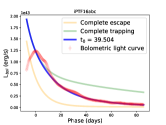
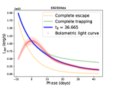
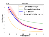
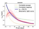
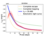
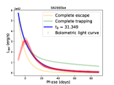
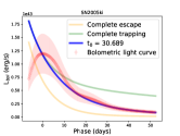
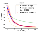
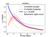
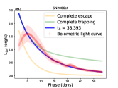
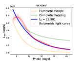
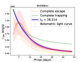
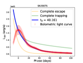
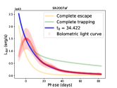
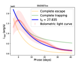
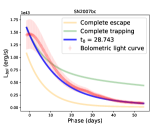
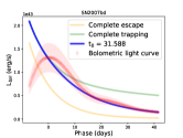
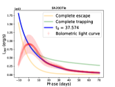
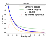
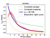
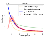
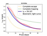
Figure 9: The radioactive decay energy deposition fits to the bolometric light curve for the sample of SNe analysed in this study. For each SN the fits are presented along with the constructed light curve and the deposition function for complete trapping and complete escape of $\gamma$-rays.

References

- Amanullah & Goobar (2011) Amanullah R., Goobar A., 2011, ApJ, 735, 20
- Arnett (1982) Arnett W. D., 1982, ApJ, 253, 785
- Ashall et al. (2018) Ashall, C., Mazzali, P. A., Stritzinger, M. D., et al. 2018, MNRAS,
- Biscardi et al. (2012) Biscardi I., et al., 2012, A&A, 537, A57
- Blondin et al. (2012) Blondin, S., Matheson, T., Kirshner, R. P., et al. 2012, AJ, 143, 126
- Blondin et al. (2013) Blondin S., Dessart L., Hillier D. J., Khokhlov A. M., 2013, MNRAS, 429, 2127
- Blondin, Dessart, & Hillier (2015) Blondin S., Dessart L., Hillier D. J., 2015, MNRAS, 448, 2766
- Blondin et al. (2017) Blondin S., Dessart L., Hillier D. J., Khokhlov A. M., 2017, MNRAS, 470, 157
- Bloom et al. (2012) Bloom J. S., et al., 2012, ApJ, 744, L17
- Bulla et al. (2018) Bulla, M., Goobar, A., Amanullah, R., Feindt, U., & Ferretti, R. 2018, MNRAS, 473, 1918
- Burns et al. (2011) Burns C. R., et al., 2011, AJ, 141, 19
- Burns et al. (2014) Burns C. R., et al., 2014, ApJ, 789, 32
- Cao et al. (2015) Cao Y., et al., 2015, Natur, 521, 328
- Cardelli, Clayton & Mathis (1989) Cardelli J. A., Clayton G. C., Mathis J. S., 1989, ApJ, 345, 245
- Cescutti & Kobayashi (2017) Cescutti, G., & Kobayashi, C. 2017, arXiv:1708.09308
- Childress et al. (2015) Childress, M. J., Hillier, D. J., Seitenzahl, I., et al. 2015, MNRAS, 454, 3816
- Contardo, Leibundgut, & Vacca (2000) Contardo G., Leibundgut B., Vacca W. D., 2000, A&A, 359, 876
- Contreras et al. (2010) Contreras C., et al., 2010, AJ, 139, 519
- Contreras et al. (2018) Contreras, C., Phillips, M. M., Burns, C. R., et al. 2018, arXiv:1803.10095
- Dhawan et al. (2015) Dhawan S., Leibundgut B., Spyromilio J., Maguire K., 2015, MNRAS, 448, 1345
- Dhawan et al. (2016) Dhawan, S., Leibundgut, B., Spyromilio, J., & Blondin, S. 2016, A&A, 588, A84
- Dhawan et al. (2017) Dhawan S., Leibundgut B., Spyromilio J., Blondin S., 2017, A&A, 602, A118
- Elias et al. (1981) Elias, J. H., Frogel, J. A., Hackwell, J. A., Persson, E. E., 1981, ApJ, 251, L13
- Elias et al. (1985) Elias J. H., Matthews K., Neugebauer G., Persson S. E., 1985, ApJ, 296, 379
- Ferretti et al. (2017) Ferretti R., et al., 2017, A&A, 606, A111
- Filippenko et al. (1992) Filippenko, A. V., Richmond, M. W., Matheson, T., et al. 1992, ApJ, 384, L15
- Fink et al. (2010) Fink M., Röpke F. K., Hillebrandt W., Seitenzahl I. R., Sim S. A., Kromer M., 2010, A&A, 514, A53
- Fink et al. (2014) Fink M., et al., 2014, MNRAS, 438, 1762
- Fisher & Jumper (2015) Fisher, R., & Jumper, K. 2015, ApJ, 805, 150
- Folatelli et al. (2012) Folatelli, G., Phillips, M. M., Morrell, N., et al. 2012, ApJ, 745, 74
- Folatelli et al. (2013) Folatelli, G., Morrell, N., Phillips, M. M., et al. 2013, ApJ, 773, 53
- Fransson & Jerkstrand (2015) Fransson, C., Jerkstrand, A., 2015, ApJ, 814, L2
- Friedman et al. (2015) Friedman A. S., et al., 2015, ApJS, 220, 9
- Ganeshalingam, Li, & Filippenko (2011) Ganeshalingam M., Li W., Filippenko A. V., 2011, MNRAS, 416, 2607
- Garavini et al. (2004) Garavini, G., Folatelli, G., Goobar, A., et al. 2004, AJ, 128, 387
- Goldstein & Kasen (2018) Goldstein, D. A., & Kasen, D. 2018, arXiv:1801.00789
- Gómez & López (1998) Gómez, G., & López, R. 1998, AJ, 115, 1096
- Goobar et al. (2015) Goobar, A., Kromer, M., Siverd, R., et al. 2015, ApJ, 799, 106
- Goobar et al. (2014) Goobar, A., Johansson, J., Amanullah, R., et al. 2014, ApJ, 784, L12
- Graham et al. (2017) Graham M. L., et al., 2017, arXiv, arXiv:1708.07799
- Hamuy et al. (1996) Hamuy M., Phillips M. M., Suntzeff N. B., Schommer R. A., Maza J., Smith R. C., Lira P., Aviles R., 1996, AJ, 112, 2438
- Hillebrandt et al. (2013) Hillebrandt W., Kromer M., Röpke F. K., Ruiter A. J., 2013, FrPhy, 8, 116
- Hosseinzadeh et al. (2017) Hosseinzadeh G., et al., 2017, ApJ, 845, L11
- Hoyle & Fowler (1960) Hoyle F., Fowler W. A., 1960, ApJ, 132, 565
- Jeffery (1999) Jeffery D. J., 1999, astro, arXiv:astro-ph/9907015
- Jiang et al. (2017) Jiang, J.-A., Doi, M., Maeda, K., et al. 2017, Nature, 550, 80
- Kasen (2006) Kasen D., 2006, ApJ, 649, 939
- Kasen (2010) Kasen D., 2010, ApJ, 708, 1025
- Kromer et al. (2013) Kromer, M., Fink, M., Stanishev, V., et al. 2013, MNRAS, 429, 2287
- Kromer et al. (2016) Kromer M., et al., 2016, MNRAS, 459, 4428
- Kromer, Ohlmann, & Roepke (2017) Kromer M., Ohlmann S. T., Roepke F. K., 2017, arXiv, arXiv:1706.09879
- Lair et al. (2006) Lair J. C., Leising M. D., Milne P. A., Williams G. G., 2006, AJ, 132, 2024
- Leibundgut (1988) Leibundgut B., 1988, PhDT,
- Maeda et al. (2011) Maeda, K., Leloudas, G., Taubenberger, S., et al. 2011, MNRAS, 413, 3075
- Magee et al. (2018) Magee, M. R., Sim, S. A., Kotak, R., & Kerzendorf, W. E. 2018, arXiv:1803.04436
- Maguire et al. (2014) Maguire, K., Sullivan, M., Pan, Y.-C., et al. 2014, MNRAS, 444, 3258
- Maguire et al. (2016) Maguire K., Taubenberger S., Sullivan M., Mazzali P. A., 2016, MNRAS, 457, 3254
- Mandel et al. (2009) Mandel K. S., Wood-Vasey W. M., Friedman A. S., Kirshner R. P., 2009, ApJ, 704, 629
- Maoz, Mannucci, & Nelemans (2014) Maoz D., Mannucci F., Nelemans G., 2014, ARA&A, 52, 107
- Marion et al. (2016) Marion G. H., et al., 2016, ApJ, 820, 92
- Matheson et al. (2008) Matheson, T., Kirshner, R. P., Challis, P., et al. 2008, AJ, 135, 1598
- Mazzali et al. (1995) Mazzali, P. A., Danziger, I. J., & Turatto, M. 1995, A&A, 297, 509
- Mazzali, et al. (1997) Mazzali, P. A., Chugai, N., Turatto, M., et al. 1997, MNRAS, 284, 151.
- Mazzali et al. (1998) Mazzali, P. A., Cappellaro, E., Danziger, I. J., Turatto, M., & Benetti, S. 1998, ApJ, 499, L49
- Mazzali et al. (2014) Mazzali, P. A., Sullivan, M., Hachinger, S., et al. 2014, MNRAS, 439, 1959
- Miller et al. (2018) Miller, A. A., Cao, Y., Piro, A. L., et al. 2018, ApJ, 852, 100
- Noebauer et al. (2017) Noebauer U. M., Kromer M., Taubenberger S., Baklanov P., Blinnikov S., Sorokina E., Hillebrandt W., 2017, MNRAS, 472, 2787
- Nugent et al. (2011) Nugent P. E., et al., 2011, Natur, 480, 344
- Pakmor et al. (2010) Pakmor R., Kromer M., Röpke F. K., Sim S. A., Ruiter A. J., Hillebrandt W., 2010, Nature, 463, 61
- Pakmor et al. (2012) Pakmor R., Kromer M., Taubenberger S., et al., 2012, ApJ, 747, L10
- Parrent et al. (2011) Parrent, J. T., Thomas, R. C., Fesen, R. A., et al. 2011, ApJ, 732, 30
- Pereira et al. (2013) Pereira, R., Thomas, R. C., Aldering, G., et al. 2013, A&A, 554, A27
- Phillips et al. (1992) Phillips, M. M., Wells, L. A., Suntzeff, N. B., et al. 1992, AJ, 103, 1632
- Piro, Chang, & Weinberg (2010) Piro A. L., Chang P., Weinberg N. N., 2010, ApJ, 708, 598
- Rabinak, Livne, & Waxman (2012) Rabinak I., Livne E., Waxman E., 2012, ApJ, 757, 35
- Ruiz-Lapuente et al. (1992) Ruiz-Lapuente, P., Cappellaro, E., Turatto, M., et al. 1992, ApJ, 387, L33
- Sahu et al. (2008) Sahu, D. K., Tanaka, M., Anupama, G. C., et al. 2008, ApJ, 680, 580-592
- Sasdelli et al. (2014) Sasdelli, M., Mazzali, P. A., Pian, E., et al. 2014, MNRAS, 445, 711
- Scalzo et al. (2014) Scalzo R., et al., 2014, MNRAS, 440, 1498
- Schlafly & Finkbeiner (2011) Schlafly E. F., Finkbeiner D. P., 2011, ApJ, 737, 103
- Seitenzahl et al. (2013) Seitenzahl I. R., et al., 2013, MNRAS, 429, 1156
- Seitenzahl et al. (2016) Seitenzahl I. R., et al., 2016, A&A, 592, A57
- Shen et al. (2017) Shen, K. J., Kasen, D., Miles, B. J., & Townsley, D. M. 2017, arXiv:1706.01898
- Silverman et al. (2012) Silverman, J. M., Foley, R. J., Filippenko, A. V., et al. 2012, MNRAS, 425, 1789
- Silverman, Ganeshalingam, & Filippenko (2013) Silverman J. M., Ganeshalingam M., Filippenko A. V., 2013, MNRAS, 430, 1030
- Sim et al. (2010) Sim S. A., et al., 2010, ApJ, 714, L52
- Stritzinger et al. (2006) Stritzinger M., Leibundgut B., Walch S., Contardo G., 2006, A&A, 450, 241
- Stritzinger & Sollerman (2007) Stritzinger M., Sollerman J., 2007, A&A, 470, L1
- Stritzinger et al. (2011) Stritzinger M. D., et al., 2011, AJ, 142, 156
- Swartz, Sutherland, & Harkness (1995) Swartz D. A., Sutherland P. G., Harkness R. P., 1995, ApJ, 446, 766
- Taubenberger et al. (2015) Taubenberger, S., Elias-Rosa, N., Kerzendorf, W. E., et al. 2015, MNRAS, 448, L48
- Wilk, Hillier, & Dessart (2017) Wilk K., Hillier D. J., Dessart L., 2017, arXiv, arXiv:1711.00105
- Woosley & Kasen (2011) Woosley S. E., Kasen D., 2011, ApJ, 734, 38
- Wygoda, Elbaz, & Katz (2017) Wygoda N., Elbaz Y., Katz B., 2017, arXiv, arXiv:1711.00969
- Zhang et al. (2016) Zhang, J.-J., Wang, X.-F., Sasdelli, M., et al. 2016, ApJ, 817, 114
- Zheng et al. (2014) Zheng, W., Shivvers, I., Filippenko, A. V., et al. 2014, ApJ, 783, L24
- Zheng et al. (2013) Zheng, W., Silverman, J. M., Filippenko, A. V., et al. 2013, ApJ, 778, L15