Entanglement Protection via Periodic Environment Resetting
in continuous-time Quantum Dynamical Processes

Abstract

The temporal evolution of entanglement between a noisy system and an ancillary system is analyzed in the context of continuous-time open quantum system dynamics. Focusing on a couple of analytically solvable models for qubit systems, we study how Markovian and non-Markovian characteristics influence the problem, discussing in particular their associated entanglement-breaking regimes. These performances are compared with those one could achieve when the environment of the system is forced to return to its input configuration via periodic instantaneous resetting procedures.

I Introduction

The preservation of entanglement is a fundamental requirement for the development of realistic applications in quantum communication COMM1 , quantum computation NIELSEN , and quantum cryptography CRYPTO . According to quantum mechanics, two entangled systems exhibit extraordinary, but fragile, correlations that are beyond any classical description ENT . A key objective in the development of reliable quantum technologies is to identify strategies which would prevent the deterioration of such exotic correlations. A plethora of different strategies have been devised to tackle this delicate issue, spanning from distillation protocols DIST , pre- and postprocessing operations ERR1 ; ERR2 ; ERR3 ; ERR4 , decoherence-free subspaces DEC ; DEC2 , to dynamical decoupling and control techniques DYNA1 ; DYNA2 ; DYNA3 ; FacchiLidar ; maniscalco-2008 ; cuevas-2017 ; CONTROL1 . All these approaches, however, are uneffective if the noise level affecting the system surpasses a certain minimal threshold that leads to entanglement-breaking (EB) dynamics horodecki-2003 . A quantum process is said to be EB if any initial amount of entanglement established between the system, evolving under the action of the noise, and an arbitrary external ancilla is destroyed. Such transformations behave essentially as classical measure-and-reprepear operations M&R and have been the subject of extensive investigation within the quantum information community; see, e.g., Refs.horodecki-2003 ; chruscinski-2006 . Determining when the EB threshold is approached during a given dynamical evolution is clearly an important facet for the construction of procedures which are more effective in the protection of quantum coherence; see, e.g., Ref. Gatto18 . The present work focuses on this task by studying the continuous-time evolution of a qubit whose dynamics are described by generalized master equations that admit explicit integration and allow one to probe both Markovian and non-Markovian regimes. While justified in certain contexts, the Markov approximation fails when the system-environment interaction leads to long-lasting and non-negligible correlations breuer-2002 . Indeed, in general, the dynamics of an open system are non-Markovian NMDOQS ; ReviewRHP , i.e., they are affected by memory effects which may lead to a reappearance of entanglement after its disappearance bellomo-2007 ; mazzola2009 . This nonmonotonic behavior of the entanglement between a system and an ancilla was indeed proposed in Ref. NMRHP as a non-Markovianity witness. Generally speaking, it can also happen that entanglement revives a long time after its sudden death or that, due to correlations with the environment, the phenomenon of entanglement trapping occurs enttrap , resulting in a highly nontrivial temporal dependence of the entanglement evolution.

In the first part of the paper we shall review the above effects, linking them to the EB analysis of the system dynamics. We then proceed by introducing a method which, with minimal control on the system environment, allows one to substantially modify the EB dynamical response. The scheme we propose takes inspiration from the notion of amendable channels introduced in Ref. anto and subsequently developed in Refs. depasquale-2013 ; CUEVAS1 ; porzio ; cuevas-2017 . Formally speaking, an amendable channel is an EB process resulting from the temporal concatenation of a collection of subprocesses, such that there exists a (typically unitary) filtering transformation acting on the system of interest in a bang-bang control fashion, which applied between the subchannels enables one to create a new effective evolution which is no longer EB. In our case we adapt this idea to the continuous-time evolution of a qubit, by assuming that we indirectly perturb its dynamics via periodic, instantaneous resettings of its environment. It is worth stressing that, at odds with the approaches of Refs. cuevas-2017 ; anto ; depasquale-2013 ; CUEVAS1 ; porzio , our scheme assumes partial control on the environment, which, in general, may not be granted. Still there are several reasons to study this procedure. First, there are configurations where the resetting assumption is an available option. For instance, in the amplitude-damping scheme describing the interaction of a two-level system $A$ with a bosonic reservoir at zero temperature (a model we analyze in Sec. III.1), the resetting merely accounts for periodically removing all the excitations that leaked out from $A$ (e.g., by means of ancillary systems that act as effective photonic sinks), or by preventing them from being reabsorbed from $A$ (e.g., by instantaneously detuning the latter). Second, the environment-resetting assumption is interesting because, despite the fact that it explicitly contrasts the back-flow of information from the bath to $A$, thereby apparently increasing the overall noise level of the dynamics, in certain regimes it allows us to improve the entanglement survival time of the model. Finally, from a mathematical point of view the resetting assumption results in a huge simplification of the problem ,as without it, it would be impossible to write the perturbed evolution of the system in a compact, treatable form, at least for non-Markovian processes.

The paper is structured as follows. In Sec. II we review the formal definitions of non-Markovian quantum-dynamical processes and of EB quantum maps. In Sec. III we present a couple of dynamical processes for qubit systems and discuss their EB properties. The environment-resetting procedure is presented in Sec. IV. Finally, we discuss our results and illustrate their possible connection with the quantum Zeno and inverse quantum Zeno effects in Sec. V. Technical material is presented in the appendices.

II Definitions

In this section we review some basic facts about open quantum system dynamics and their characterization in terms of Markovian and non-Markovian models, and introduce the formal definition of EB channels.

II.1 Continuous-time open quantum processes

In the continuous-time approach the dynamics of an open quantum system $A$ are described by a $t$-parametrized family $\{\Phi_{0\rightarrow t}\}_{t\geq 0}$ of completely positive (CP), trace-preserving maps (quantum channels) that link a generic input state $\varrho^{A}(0)$ of the system to its temporal evolved counterpart $\varrho^{A}(t)$ via the mapping

$$\varrho^{A}(t)=\Phi_{0\rightarrow t}(\varrho^{A}(0))\;.$$ (1)

In this setting, time-homogenous Markovian dynamics can be associated to the semigroup property

$$\Phi_{0\rightarrow t}=\Phi_{0\rightarrow t-s}\circ\Phi_{0\rightarrow s}\;,\qquad\mbox{$\forall t$ and $\forall s\leq t$,}$$ (2)

with “$\circ$” representing the composition of maps, i.e., $\Phi_{0\rightarrow t-s}\circ\Phi_{0\rightarrow s}(\varrho)=\Phi_{0\rightarrow t-s}(\Phi_{0\rightarrow s}(\varrho))$. Equivalently, we can associate these dynamics to the Gorini-Kossakowski-Sudarshan-Lindblad (GKSL) form of the master equation Lindblad ; GKS , which describes the evolution of the system’s density matrix in terms of time-independent Hamiltonian $H$ and dissipator ${\cal D}$,

$$\frac{\partial}{\partial t}\varrho^{A}(t) = -i[H,\varrho^{A}(t)]+{\cal D}(\varrho^{A}(t))\;,$$ (3)

$${\cal D}(\cdot) = \sum_{j}\left(L_{j}\cdot L_{j}^{\dagger}-\frac{1}{2}\{L_{j}^{\dagger}L_{j},\cdot\}\right)\;,$$ (4)

with $[\cdot,\cdot]$ and $\{\cdot,\cdot\}$ being the commutator and anticommutator, respectively, and $L_{j}$ the Lindblad operators.

Starting from a microscopic model of the system, environment, and interaction, the enforcement of condition (2) on the system’s dynamics requires a number of assumptions, such as system-reservoir weak coupling breuer-2002 . In certain physical contexts, however, such approximations are unjustified, and one needs to go beyond perturbation theory. A straightforward extension of the semigroup property (2) is the notion of divisibility. A dynamical map is CP-divisible, or simply divisible, iff the propagator $\Lambda_{s\rightarrow t}$ defined through the expression

$$\Phi_{0\rightarrow t}=\Lambda_{s\rightarrow t}\circ\Phi_{0\rightarrow s}\;,$$ (5)

is CP, $\forall t$ and $\forall s\leq t$. This amounts to saying that the evolution of $A$ can be described at all times as a concatenation of quantum channels, a condition which allows us to still write a linear differential equation for $\varrho^{A}(t)$ as in (3) with explicitly time-dependent operators $H(t)$ and $L_{j}(t)$. Of course, systems obeying (2) can be seen as special instances of divisible models with CP propagators $\Lambda_{s\rightarrow t}$ that also fulfill the constraint

$$\Lambda_{s\rightarrow t}=\Lambda_{0\rightarrow t-s}\;,\qquad\mbox{$\forall t$ and $\forall s\leq t$,}$$ (6)

which explains why we dubbed them as “time-homogenous Markovian” instead of simply Markovian processes. Any process whose dynamics are not divisible are considered non-Markovian.

A non-Markovianity measure quantifying the deviation from divisibility has been proposed in NMRHP whose physical interpretation has only very recently been fully unveiled BognaToni . Specifically Ref. NMRHP introduces a witness of nondivisibility which exploits the temporal evolution of the entanglement between the open system state and an external ancilla: a nonmonotonic decay of such entanglement indicates nondivisibility, and therefore non-Markovianity, of the dynamical map. A different perspective on the definition of non-Markovianity is to interpret memory effects in terms of information back-flow. This path was first undertaken by Breuer, Laine, and Piilo by quantifying the information content of an open quantum system in terms of distinguishability between pairs of states NMBLP . Several other information-theoretic measures of non-Markovianity have been proposed in the last decade ReviewRHP ; NMDOQS . The key property exploited in these definitions is that the time evolution of a given quantifier of information suitable to describe memory effects, e.g., distinguishability between quantum states, is contractive under CP maps. Hence a temporary increase of distinguishability, which is physically interpreted as a partial increase in the information content of the open system due to memory effects, always implies that divisibility of the dynamical map is violated.

II.2 Entanglement breaking channels

A quantum channel $\Phi$ acting on a system $A$ is said to be EB horodecki-2003 if, irrespective of the choice of joint state $\varrho^{AB}$ of $A$ and of an arbitrary ancilla $B$, the associated output $(\Phi\otimes{\rm Id})(\varrho^{AB})$ is separable, ${\rm Id}$ indicating the identity channel on $B$. For finite dimensional systems the Choi-Jamiołkowski isomorphism choij ; JAM allows us to restrict the analysis to the case where $B$ is isomorphic to $A$ and $\varrho^{AB}$ is the maximally entangled state $|\Omega\rangle_{AB}=\frac{1}{\sqrt{d}}\sum_{k=1}^{d}|k\rangle_{A}\!\otimes|k\rangle_{B}$, $\{|k\rangle\}_{k=1,\cdots,d}$ being an orthonormal basis on the associated Hilbert space. Such an output density matrix $\varrho^{AB}_{\Phi}=(\Phi\otimes{\rm Id})(|\Omega\rangle_{AB}\langle\Omega|)$ is called the Choi-Jamiołkowski (CJ) state of $\Phi$, and its separability is equivalent to the EB property of the map. In what follows we shall focus on the case where $A$ is a qubit system. Accordingly we identify $|\Omega\rangle_{AB}$ with the Bell state $\tfrac{1}{\sqrt{2}}(|00\rangle+|11\rangle)$, and use the concurrence wootters-1998 of the CJ state as a necessary and sufficient instrument to determine whether or not the associated map is EB. We remind the reader that given a two-qubit state $\varrho^{AB}$, its concurrence ${C}[\varrho^{AB}]\in[0,1]$ is a proper entanglement measure which assumes nonzero values if and only if $\varrho^{AB}$ is entangled. It can be computed as

$$C[\varrho^{AB}]=\max\{0,\sqrt{\varepsilon_{1}}-\sqrt{\varepsilon_{2}}-\sqrt{\varepsilon_{3}}-\sqrt{\varepsilon_{4}}\},$$ (7)

where $\{\varepsilon_{i}\}_{i=1}^{4}$ is the set of eigenvalues (in descending order) of the operator $\chi=\varrho^{AB}(\sigma_{2}^{A}\otimes\sigma_{2}^{B})\varrho^{AB*}(\sigma_{2}^{A}\otimes\sigma_{2}^{B})$, with $\varrho^{AB*}$ the complex conjugate of $\varrho^{AB}$ and $\sigma^{X}_{2}$ being the second Pauli matrix acting on the system $X=A,B$.

III EB properties of dynamical processes acting on a qubit

In this section we present a couple of examples of dynamical processes $\{\Phi_{0\rightarrow t}\}_{t\geq 0}$ for a qubit system which are exactly solvable and which, depending on the model parameters, allow one to describe both Markovian and non-Markovian evolutions. In particular we are interested in studying their EB properties as a function of the temporal index $t$. According to the previous section this can be done by looking at the zeros of the concurrence $C(t)$ of the CJ state

$$\varrho^{AB}_{\Phi_{0\rightarrow t}}=({\Phi_{0\rightarrow t}}\otimes\mathrm{Id})(|\Omega\rangle_{AB}\langle\Omega|)$$ (8)

of the map $\Phi_{0\rightarrow t}$, i.e., by solving the equation

$$C(t)={C}[\varrho^{AB}_{\Phi_{0\rightarrow t}}]=0\;.$$ (9)

For divisible processes, due to the CP property of the propagator $\Lambda_{s\rightarrow t}$ of Eq. (5), the function $C(t)$ is explicitly nonincreasing. Therefore, after the concurrence reaches zero, it remains that value for all subsequent instants  Gatto18 . By contrast, in the general non-Markovian setting this is not necessarily true as the associated function $C(t)$ can be explicitly nondecreasing due to information back-flow. However, notice that, as previously mentioned, since the nonmonotonic behavior of entanglement measures is only a witness of non-Markovianity NMRHP , there exist non-Markov processes which still admit nonincreasing $C(t)$, e.g., when the propagator $\Lambda_{s\rightarrow t}$ of the family is just positive but not CP PDIVISIBILITY .

III.1 Time-local amplitude-damping channels

As a first case study we consider an amplitude-damping channel for a two-level atom (qubit) $A$, whose density matrix evolves according to the time-local differential master equation

$$\dfrac{d\varrho^{A}(t)}{dt}=\gamma(t)\left(\sigma_{-}\varrho^{A}(t)\sigma_{+}-\dfrac{1}{2}\{\sigma_{+}\sigma_{-},\varrho^{A}(t)\}\right),$$ (10)

where $\sigma_{\pm}=\frac{1}{2}(\sigma_{1}\pm i\sigma_{2})$ are the raising and lowering operators of the system. In this expression the function $\gamma(t)$ is an effective (time-dependent) rate, which, as will become clear in a moment, need not be positive semidefinite at all times. Equation (10) admits an analytical integration whose solution, expressed in the eigenbasis $\{|0\rangle_{A},|1\rangle_{A}\}$ of the $\sigma_{3}$ Pauli operator, results in

$$\varrho^{A}(t)=\begin{pmatrix}\varrho^{A}_{11}(0)P(t)&\varrho^{A}_{10}(0)\sqrt{P(t)}\\ \varrho^{A}_{01}(0)\sqrt{P(t)}&\varrho^{A}_{00}(0)+\varrho^{A}_{11}(0)(1-P(t))\end{pmatrix},$$ (11)

with

$$P(t):=e^{-\Gamma(t)},\qquad\Gamma(t):=\int_{0}^{t}dt^{\prime}\gamma(t^{\prime})\;,$$ (12)

representing the population of the level $|1\rangle_{A}$. The above expressions clarify the condition that the rate $\gamma(t)$ has to fulfill in order to interpret Eq. (11) as an instance of Eq. (1) for a proper choice of the quantum channel $\Phi_{0\rightarrow t}$: indeed, exploiting the fact that a necessary and sufficient CP condition for (11) is to have the function $P(t)$ be positive and no larger than 1, it follows that Eq. (10) is a legitimate dynamical equation for $A$ if and only if the function $\gamma(t)$ respects the constraint

$$\Gamma(t)\geq 0\;,\qquad\forall t\geq 0\;.$$ (13)

Equation (13) is clearly fulfilled if we enforce the positivity condition directly on $\gamma(t)$. Under this restriction Eq. (10) is explicitly in the generalized GKSL form, characterized by a single time-dependent Linbdlad operator $L(t)=\sqrt{\gamma(t)}\sigma_{-}$, and the resulting process is divisible. Furthermore, if we take the rate to be positive and constant $\gamma(t)=\lambda$, then the maps $\Phi_{0\rightarrow t}$ become time-homogeneous, yielding a population $P(t)$ which is exponentially decreasing:

$$P(t)=e^{-\lambda t}\;.$$ (14)

Finally, if $\gamma(t)$ assumes negative values [while still fulfilling (13)] the resulting process is non-Markovian as we explicitly show next.

Indeed, by direct evaluation one can verify that the CJ state (8) of the model has the following $X$-shaped form:

$$\varrho^{AB}_{\Phi_{0\rightarrow t}}=\dfrac{1}{2}\begin{pmatrix}P(t)&0&0&\sqrt{P(t)}\\ 0&0&0&0\\ 0&0&1-P(t)&0\\ \sqrt{P(t)}&0&0&1\end{pmatrix},$$ (15)

whose concurrence can be explicitly computed ERR4 resulting in the expression

$$C(t)=\sqrt{P(t)}=e^{-\Gamma(t)/2}$$ (16)

(see Appendix A for details). Taking the derivative and invoking Eq. (12), we now have

$$\frac{d}{dt}C(t)=-\frac{\sqrt{P(t)}}{2}\gamma(t),$$ (17)

which shows that a negative value of $\gamma(t)$ implies an increasing behavior for $C(t)$ and, as anticipated, a non-Markovian character of the system’s dynamics via a direct application of the sufficient condition of Ref. NMRHP .

Equation (17) can also be used to directly link the EB properties of the process to the probability $P(t)$: in particular we notice that the system becomes EB for those times $t$ where $P(t)$ reaches zero, or equivalently where $\Gamma(t)$ explodes:

$$\Phi_{0\rightarrow t}\in{\rm EB}\Longleftrightarrow P(t)=0\;.$$ (18)

For the case of the time-homogenous Markovian evolution this immediately tells us that the system reaches the EB regime only in the asymptotic limit $t\rightarrow\infty$. A less trivial example can be found when studying the interaction of a two-level system $A$ with a bosonic reservoir at zero temperature characterized by a Lorentzian spectral density, $J(\omega):=\dfrac{1}{2\pi}\dfrac{\alpha\ell^{2}}{(\omega_{0}-\omega)^{2}+\ell^{2}}$ with $\alpha\geq 0$ the effective coupling constant, $\ell$ the width of the Lorentzian spectrum, and the frequency $\omega_{0}$ gauging the energy gap of $A$; see, e.g., Refs. breuer-2002 ; NMBLP . Under this condition one can show that the probability $P(t)$ gets expressed as

$$P(t)=e^{-\ell t}\left[\cos\left(\dfrac{\Delta\;t}{2}\right)+\dfrac{\ell}{\Delta}\sin\left(\dfrac{\Delta\;t}{2}\right)\right]^{2}\;,$$ (19)

with

$$\Delta:=\sqrt{\ell(2\alpha-\ell)}\;.$$ (20)

A close inspection of these equations reveals that when $\alpha/\ell\leq 1/2$ the excited state probability $P(t)$ decays monotonically to zero, reaching such a value only asymptotically. As shown in Ref. NMBLP , in this case the information, as measured, e.g., by state distinguishability, flows from system to environment: accordingly, in agreement with our previous observation, the dynamics are divisible, and the system becomes EB only at infinite time. In the opposite parameter regime, i.e., when $\alpha/\ell>1/2$, $P(t)$ has an oscillatory behavior vanishing at times

$$\tau_{k}:=\frac{2}{\Delta}(k\pi-\arctan(\Delta/\ell)),$$ (21)

with $k\geq 1$ an integer. Memory effects in this case kick in and appear as information back-flow, divisibility is lost, and the dynamics are non-Markovian NMBLP . Accordingly $C(t)$ acquires an oscillating behavior, periodically reaching zero at the special times (21) where the process becomes instantaneously EB; see Fig. 1.

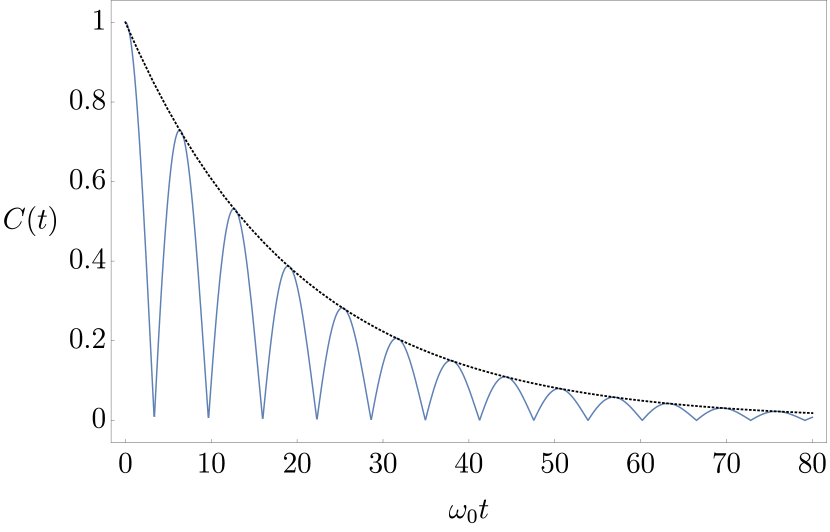
Figure 1: (Color online) Time evolution of the CJ concurrence (16) of the amplitude-damping channel (11) characterized by probability $P(t)$ of Eq. (19), in the non-Markovian regime with $\alpha=5\omega_{0}$ and $\ell=0.1\omega_{0}$ (blue solid line). The black dotted line on top corresponds to the exponential envelope of the curve, i.e., the function $e^{-\ell t/2}$ which incidentally corresponds to the CJ concurrence of the time-homogenous Markovian process of Eq. (14) with constant rate $\lambda=\ell$.

III.2 Time-local Pauli channels

As a second example of a continuous-time quantum process, we consider the case of a qubit evolving under the action of the following time-local Pauli channel, described by the master equation

$$\dfrac{d\varrho^{A}(t)}{dt}=\frac{1}{2}\sum_{k=1}^{3}\gamma_{k}(t)(\sigma_{k}\varrho^{A}(t)\sigma_{k}-\varrho^{A}(t)),$$ (22)

where $\gamma_{k}(t)$ are time-dependent decay rates fulfilling the inequalities

$$\Gamma_{k}(t):=\int_{0}^{t}\gamma_{k}(t^{\prime})dt^{\prime}\geq 0\;,\qquad\forall k=1,2,3.$$ (23)

Analogously to Eq. (13) in the previous section, the above is a necessary and sufficient condition to guarantee the complete positivity of the associated dynamical maps $\Phi_{0\rightarrow t}$ of the process, which by direct integration can be expressed as a sum of unitary transformations applied to $A$. Specifically defining $\beta_{i}(t):=\exp[-\Gamma_{j}(t)-\Gamma_{k}(t)]$ for $i\neq j\neq k$ and introducing the functions

$$p_{1}(t) :=\frac{1}{4}\left[1-\beta_{3}(t)-\beta_{2}(t)+\beta_{1}(t)\right],$$ (24)

$$p_{2}(t) :=\frac{1}{4}\left[1-\beta_{3}(t)+\beta_{2}(t)-\beta_{1}(t)\right],$$ (25)

$$p_{3}(t) :=\frac{1}{4}\left[1+\beta_{3}(t)-\beta_{2}(t)-\beta_{1}(t)\right],$$ (26)

and

$$p_{0}(t) := 1-\sum_{k=1}^{3}p_{k}(t)$$ (27)

$$= \frac{1}{4}\left[1+\beta_{3}(t)+\beta_{2}(t)+\beta_{1}(t)\right],$$

we can write

$$\Phi_{0\rightarrow t}(\varrho^{A}(0))=\sum_{k=0}^{3}p_{k}(t)\sigma_{k}\varrho^{A}(0)\sigma_{k},$$ (28)

where $\sigma_{0}=\openone$ is the identity matrix. In particular, assuming the $\gamma_{k}(t)$ to be equal to a given rate $\gamma(t)$, one has

$$p_{1}(t) = p_{2}(t)=p_{3}(t)=(1-e^{-2\Gamma(t)})/4\;,$$ (29)

$$p_{0}(t) = (1+3e^{-2\Gamma(t)})/4\;,$$ (30)

and the above equation reduces to

$$\Phi_{0\rightarrow t}(\varrho^{A}(0)) = p_{0}(t)\varrho^{A}(0)+\frac{1-p_{0}(t)}{3}\sum_{k=1}^{3}\sigma_{k}\varrho^{A}(0)\sigma_{k},$$ (31)

$$= \eta(t)\varrho^{A}(0)+\frac{1-\eta(t)}{2}\openone,$$

which describes a qubit depolarizing channel NIELSEN ; KING with noisy parameter

$$\eta(t):=\frac{4p_{0}(t)-1}{3}=e^{-2\Gamma(t)},$$ (32)

[in deriving this expression we use the identity $\sum_{k=0}^{3}\sigma_{k}\varrho^{A}(0)\sigma_{k}=2\openone$].

As in the amplitude-damping model, Eq. (22) allows us to describe different regimes. In particular if the $\gamma_{k}(t)$ are taken to be positive semidefinite, then the associated dynamics are provably divisible, with Eq. (22) being explicitly in the GKSL form with three time-dependent generators $L_{k}(t)=\sqrt{\gamma_{k}(t)/2}\;\sigma_{k}$ (the time-homogeneous limit being reached when further imposing the rates to be constant). Non-Markovian behaviors can instead be obtained by allowing the rates $\gamma_{k}(t)$ to assume negative values while still respecting the constraint (23).

Following the same derivation as the previous section, the CJ state of the Pauli channel model can be written as

$$\varrho^{AB}_{\Phi_{0\rightarrow t}}=$$ (33)

$$\frac{1}{4}\begin{pmatrix}1+\beta_{3}(t)&0&0&\beta_{1}(t)+\beta_{2}(t)\\ 0&1-\beta_{3}(t)&\beta_{1}(t)-\beta_{2}(t)&0\\ 0&\beta_{1}(t)-\beta_{2}(t)&1-\beta_{3}(t)&0\\ \beta_{1}(t)+\beta_{2}(t)&0&0&1+\beta_{3}(t))\end{pmatrix},$$

with a CJ concurrence (9) equal to

$$C(t)=\max\{0,2p_{0}(t)-1\},$$ (34)

which we now study for some paradigmatic examples of decaying rates $\gamma_{k}(t)$. The first is obtained by considering the simple Markovian scenario where they are all taken to be non-negative constants, namely, $\gamma_{k}(t)=\gamma_{k}\geq 0$. In this case it is easy to see that Pauli channels always become EB after a certain characteristic length or time: indeed by direct inspection one notices that $C(t)>0$ if and only if

$$e^{-(\gamma_{2}+\gamma_{3})t}+e^{-(\gamma_{3}+\gamma_{1})t}+e^{-(\gamma_{2}+\gamma_{1})t}>1\;,$$ (35)

a condition which is violated for sufficiently large $t$. A completely different behavior is obtained instead by assuming the rates to be

$$\gamma_{k}(t)=\gamma_{k}(1+t^{2})^{-s_{k}/2}\bar{\Gamma}(s_{k})\sin(s_{k}\arctan(t)),$$ (36)

where $\bar{\Gamma}$ is the Euler gamma function, $\gamma_{k}$ are positive coupling constants, $t$ is expressed in dimensionless units, and $s_{k}$ are the so-called Ohmicity parameters taking positive real values. These types of decay rates arise from a microscopic model of a bosonic environment with an Ohmic-class spectral density (see, e.g., Ref. haikka-2013 ), and they have been widely studied in the literature, mostly in the pure-dephasing dynamical case. Specific examples of the Ohmicity parameters $s_{k}$ are the case of the Ohmic environment $s_{k}=1$, sub-Ohmic environment $s_{k}<1$, and super-Ohmic environment $s_{k}>1$. It turns out that as long as $s_{k}\leq 2$, the model is still divisible, thereby exhibiting a Markovian character haikka-2010 . In what follows we focus on the threshold case where the three decay rates are all equal to $2$, i.e., $s_{k}=s=2$. Under this assumption the decay rates vanish after a finite time $\bar{t}$, and remain exactly zero thereafter; see Fig. 2 a). As a consequence this system experiences entanglement trapping, as illustrated in Fig. 2 b), hence the channel is never EB, contrary to the case of positive constant decay rates.

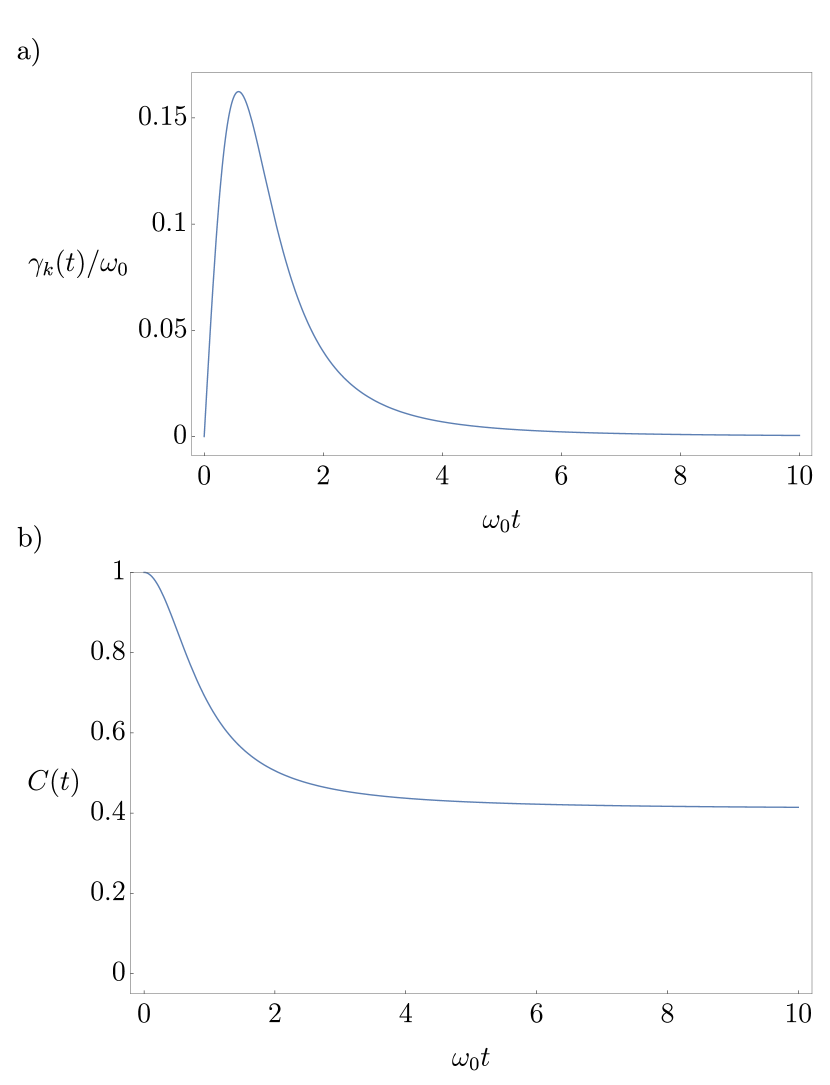
Figure 2: (Color online) a) Time-dependent decay rate $\gamma_{k}(t)$ of Eq. (36) of the Pauli channel model, with $s_{k}=2$ and $\gamma_{k}=0.25$. b) Time evolution of the associated CJ concurrence $C(t)$ of Eq. (34) with time-dependent decay rate.

We now turn our attention to the case where the Pauli channel is non-Markovian, e.g., we consider as decay rates the functions

$$\gamma_{k}(t)=\frac{2\alpha_{k}}{\sqrt{1-\tfrac{2\alpha_{k}}{\lambda_{k}}}\;\mbox{cotanh}\left(\tfrac{\lambda_{k}t}{2}\sqrt{1-\tfrac{2\alpha_{k}}{\lambda_{k}}}\right)+1}\;,$$ (37)

with $\lambda_{k}$ and $\alpha_{k}$ parameters associated to the microscopic details of the system-environment interaction. Note that, the master equation is nondivisible for $2\alpha_{k}/\lambda_{k}>1$, since in this case the decay rates take temporarily negative values. For simplicity we focus on the symmetric case $\gamma_{1}(t)=\gamma_{2}(t)=\gamma_{3}(t)$, such that $\alpha_{k}=\alpha$ and $\lambda_{k}=\lambda$ for $k=1,2,3$. Figure 3 shows that the behavior of the concurrence in this regime is similar to that of the amplitude-damping channel (see Fig. 1 for comparison). However, now there are extended intervals of transmission lengths for which entanglement is lost, while in the non-Markovian amplitude-damping case this happens only at certain times.

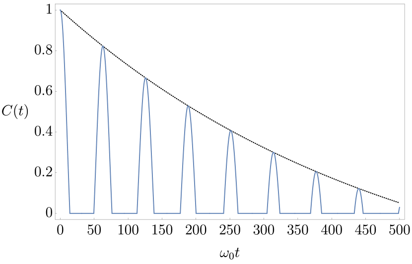
Figure 3: (Color online) CJ concurrence $C(t)$ for the Pauli channel model with uniform rates (37) as a function of time in the non-Markovian regime $2\alpha_{k}/\lambda_{k}>1$ (blue line) and the decaying envelope (black dotted line above).

IV Restoring entanglement via environment resetting

In this section we analyze what happens if during the system’s evolution, as described by a family $\{\Phi_{0\rightarrow t}\}_{t\geq 0}$, we allow for periodic resetting of its environment. Specifically the idea is to divide the temporal axis into a collection of time intervals ${\cal I}_{n}=[t_{n},t_{n+1})$ which for simplicity we assume to have uniform length $\tau=t_{n+1}-t_{n}$ and $t_{0}=0$. Then at the end of each interval we are assumed to instantaneously reset the system environment to the input state it had at the beginning of such an interval, essentially enforcing partial divisibility on the system. The resulting evolution of $A$ can be described by a new $t$-parameter family of perturbed mappings $\{\tilde{\Phi}^{(\tau)}_{0\rightarrow t}\}_{t\geq 0}$ which for $t\in{\cal I}_{n}$ are defined by the identity

$$\tilde{\Phi}^{(\tau)}_{0\rightarrow t} := \Phi_{0\rightarrow t-n\tau}\circ\overbrace{(\Phi_{0\rightarrow\tau})\circ\cdots\circ(\Phi_{0\rightarrow\tau})}^{\text{$n$ times}}$$ (38)

$$= \Phi_{0\rightarrow t-n\tau}\circ(\Phi_{0\rightarrow\tau})^{n}\;.$$

Our next step is to study how the EB properties of the problem get transformed in passing from $\Phi_{0\rightarrow t}$ to its perturbed counterpart $\tilde{\Phi}^{(\tau)}_{0\rightarrow t}$. We shall address this issue in the following subsections by applying the construction (38) to the qubit processes introduced in Sec. III. Before entering into this, however, we would like to make two remarks.

Remark 1: From the divisibility analysis presented in Sec. II.1, it should be clear that the map (38) in general does not coincide with $\Phi_{0\rightarrow t}$. A notable exception is of course provided by time-homogeneous Markovian processes fulfilling the semigroup property (2) for which the equality

$${\tilde{\Phi}}^{(\tau)}_{0\rightarrow t}={\Phi}_{0\rightarrow t}$$ (39)

trivially holds for all choices of the interval length $\tau$. For these models no advantages or disadvantages can be expected from the periodic environment-resetting strategy. In this special scenario one could however modify the scheme (38) by adding, for instance, periodic unitary rotations $U$ on $A$, along the line of the filtering scheme proposed in Refs. anto ; depasquale-2013 ; CUEVAS1 ; porzio , creating the perturbed transformations

$$\tilde{\Phi}^{(U,\tau)}_{0\rightarrow t} = \Phi_{0\rightarrow t-n\tau}\circ({\cal U}\circ\Phi_{0\rightarrow\tau})^{n}\;,$$ (40)

where ${\cal U}(\cdot)=U\cdot U^{\dagger}$ is a unitary channel; an example of this alternative approach is briefly presented in Appendix B. However, the situation already changes for those Markovian processes which are not time-homogeneous: here, due to the lack of the translational invariance property (6), one has that the perturbed evolution ${\tilde{\Phi}}^{(\tau)}_{0\rightarrow t}$ differs from the unperturbed one ${\Phi}_{0\rightarrow t}$.

Remark 2: Equation (38) admits a continuous limit when sending $\tau\rightarrow 0$ and $n\rightarrow\infty$ while keeping constant their product $n\tau\simeq t$, with $t-n\tau<\tau$. Indeed, assuming the maps $\Phi_{0\rightarrow t}$ of the original process to be continuous and differentiable at the origin of the temporal axis, we write $\Phi_{0\rightarrow\tau}\simeq{\rm Id}+\tau\;{\cal L}_{0}$, with ${\cal L}_{0}=\tfrac{\partial}{\partial t}\Phi_{0\rightarrow t}|_{t=0}$. Replacing this in Eq. (38) we obtain $\tilde{\Phi}^{(t/n)}_{0\rightarrow t}\simeq({\rm Id}+\frac{t}{n}{\cal L}_{0})^{n}$, and hence

$$\bar{\Phi}_{0\rightarrow t}:=\lim_{n\rightarrow\infty}\tilde{\Phi}^{(t/n)}_{0\rightarrow t}=e^{{\cal L}_{0}t}\;,$$ (41)

which is explicitly time-homogeneous and Markovian.

IV.1 Perturbed amplitude-damping channels

Let us first focus on the transformation (38) obtained when the unperturbed process $\Phi_{0\rightarrow t}$ is given by the amplitude-damping channel of Sec. III.1. A simple iteration of Eq. (11) reveals that in this case $\tilde{\Phi}^{(\tau)}_{0\rightarrow t}$ is still an amplitude-damping channel with a modified function $P(t)$. Specifically we have

$$\varrho^{A}(t) = \tilde{\Phi}^{(\tau)}_{0\rightarrow t}(\varrho^{A}(0))$$

$$= \begin{pmatrix}\varrho^{A}_{11}(0)\tilde{P}(t)&\varrho^{A}_{10}(0)\sqrt{\tilde{P}(t)}\\ \varrho^{A}_{01}(0)\sqrt{\tilde{P}(t)}&\varrho^{A}_{00}(0)+\varrho^{A}_{11}(0)(1-\tilde{P}(t))\end{pmatrix},$$

where for $t\in{\cal I}_{n}$, the function $\tilde{P}(t)$ is obtained from $P(t)$ of the original process through the identity

$$\tilde{P}(t)=P(t-n\tau)P^{n}(\tau)\;,$$ (43)

corresponding to a CJ concurrence equal to

$${C}(t)=\sqrt{\tilde{P}(t)}\;.$$ (44)

Notice that for $P(t)$ exponentially decreasing as in Eq. (14), we have $\tilde{P}(t)=P(t)$, which implies the identity (39) of Remark 1, in agreement with the fact that in this regime the original process is time-homogeneous and Markovian. Regarding Remark 2 instead, we observe that in the present case, by direct computation, the continuous limit process (41) is still an amplitude-damping channel of the form (11) with a probability parameter that is now given by

$$\bar{P}(t):=e^{-\bar{\lambda}t}\;,\qquad\bar{\lambda}:=-\frac{\partial}{\partial t}P(t)|_{t=0}\;.$$ (45)

As an illustrative example we now assume $P(t)$ of the unperturbed model to be as in Eq. (19). We have numerically observed that as long as $\tau$ is strictly smaller than the value $\tau_{1}$ of Eq. (21), at which point the CJ concurrence of $\Phi_{0\rightarrow t}$ reaches the zero value for the first time, the perturbed CJ concurrence (44) never vanishes, meaning that $\tilde{\Phi}^{(\tau)}_{0\rightarrow t}$ is prevented from reaching the EB regime at all times. By contrast, as soon as $\tau$ is at least as large as $\tau_{1}$ the perturbed channel acquires an EB character: in particular for $\tau=\tau_{1}$, the family $\{\tilde{\Phi}^{(\tau)}_{0\rightarrow t}\}_{t\geq 0}$ is EB for all $t\geq\tau_{1}$. Plots of the associated CJ concurrence (44) of $\tilde{\Phi}^{(\tau)}_{0\rightarrow t}$ are presented in Fig. 4 for various choices of the partition interval $\tau<\tau_{1}$ under the assumption the unperturbed evolution is non-Markovian (i.e., $\alpha/\ell>1/2$). We have compared $\tau$ with the characteristic time $\tau_{c}=1/\ell$ of the exponential decay for the unperturbed amplitude-damping model, which, for the sake of simplicity, we assume to be the smallest time scale of the problem—a possibility that can be achieved by keeping $\alpha/\ell-1/2$ positive but small. (Note that, for our considerations, $\tau_{c}<\tau_{1}$.) Under this circumstance one observes that if $\tau<\tau_{c}$ the CJ concurrence in the presence of interruptions (red line in the figure) will always be greater than the one without interruptions, reaching the constant value of $1$ as $\tau$ approaches zero. This behavior can be understood by observing that for $P(t)$ as in Eq. (19), irrespective of the parameters $\ell$ and $\alpha$, we have

$$\bar{\lambda}=\frac{\partial}{\partial t}P(t)|_{t=0}=0,\Longrightarrow\bar{P}(t)=1\;,$$ (46)

implying that in the continuous limit (41) the perturbed transformation $\tilde{\Phi}^{(\tau)}_{0\rightarrow t}$ always approaches the identity channel:

$$\bar{\Phi}_{0\rightarrow t}={\rm Id}\;.$$ (47)

As we shall comment in the conclusions, this effect can be seen as a consequence of the Zeno effect, induced by the frequent resetting of its environment facchi-2001 ; FacchiLidar .

The preceding scheme could be implemented via recursive fast cooling of the two-level system; for example, the system and its local environment could be placed within a low (near-zero) temperature fridge that is directly connected to the latter. Within this setting, every $\tau$ seconds we could open the thermal contact for a brief period.

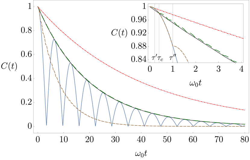
Figure 4: (Color online) Plot of the CJ concurrence (16) of the amplitude-damping evolution for $\alpha=5\omega_{0}$ and $\ell=0.1\omega_{0}$, as a function of time without interruptions to the dynamics (solid blue line) and the envelope of its peaks (dotted black line). The dynamics of CJ concurrence (44) for the perturbed map are depicted for $\tau^{\prime}<\tau_{c}$ (red dot-dashed line), $\tau^{\prime\prime}>\tau_{c}$ (dashed brown line), and for $\tau=\tau_{c}$ (wider-dashed green line). The inset shows the initial behavior of these functions.

IV.2 Perturbed depolarizing channels

We now turn our attention to the case where the qubit system is subjected to a Pauli channel with a generator given by Eq. (22) focusing on the symmetric case where the rates (37) are all identical leading to the depolarizing maps (31). By direct iteration one can easily verify that the perturbed map (38) remains a depolarizing channel with an effective noisy parameter,

$$\tilde{\Phi}^{(\tau)}_{0\rightarrow t}(\varrho^{A}(0)) = \tilde{\eta}(t)\varrho^{A}(0)+\frac{1-\tilde{\eta}(t)}{2}\mbox{Tr}[\varrho^{A}(0)]\;,$$ (48)

where for $t\in{\cal I}_{n}$ the function $\tilde{\eta}(t)$ is obtained from the $\eta(t)$ of the original process (31) through the same identity we observed in Eq. (43):

$$\tilde{\eta}(t)=\eta(t-n\tau)\eta^{n}(\tau)\;.$$ (49)

From this and from Eqs. (34) and (32), the CJ concurrence of $\tilde{\Phi}^{(\tau)}_{0\rightarrow t}$ can then be expressed in the following compact form:

$$C(t)=\mathrm{max}\Big{\{}0,\tfrac{1}{2}(3\tilde{\eta}(t)-1)\Big{\}}.$$ (50)

The continuous limit transformation (41) can also be easily computed resulting once more in a depolarizing channel with effective noisy parameter

$$\bar{\eta}(t)=e^{-\bar{\lambda}t}\;,$$ (51)

with

$$\bar{\lambda}:=-\frac{\partial\eta(t)}{\partial t}\Big{|}_{t=0}=-\frac{4}{3}\frac{\partial p_{0}(t)}{\partial t}\Big{|}_{t=0}=2\gamma(0)\;,$$ (52)

where in the last two identities we used the identity (32). Plots of (50) are reported in Fig. 5 for the case where the original rate $\gamma(t)$ of the Pauli channel is as in Eq. (37) revealing the analogous behaviors to those observed in the amplitude-damping case. Also, for this choice of $\gamma(t)$, one has $\gamma(0)=0$ and hence $\bar{\eta}(t)=1$ which implies again that the continuous limit of the perturbed map is given by the identity channel.

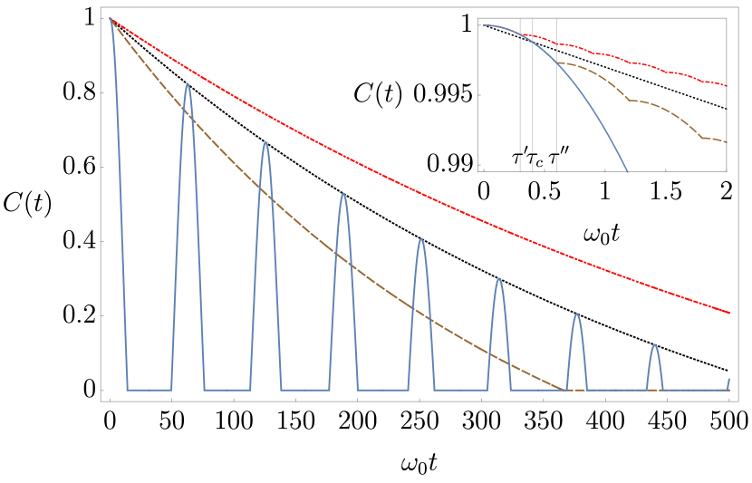
Figure 5: (Color online) Temporal evolution of the unperturbed (blue solid curve) and perturbed CJ concurrences of a depolarizing channel, for two different values of $\tau$: $\tau^{\prime}<\tau_{c}$ (red dot-dashed) and $\tau^{\prime\prime}>\tau_{c}$ (brown dashed). The dotted black curve shows the decaying envelope of the unperturbed dynamical map. The inset contains a zoom-in of the short-time behavior. All curves have been produced assuming the rates of the Pauli channel as in Eq. (37) with $\alpha_{k}=5\omega_{0}$ and $\lambda_{k}=10^{-3}$ for all $k$.

V Discussion and Conclusions

In this paper we have studied the EB character of continuous-time quantum processes. The presence of non-Markovian effects causes a nontrivial temporal dependence in the problem, as dynamics which are EB for certain times may become non-EB later on due to memory-induced entanglement revivals. In the spirit of reservoir engineering, we have also shown that EB properties can be manipulated by properly acting on the environment, e.g., via periodic resetting of its initial state. In particular, we have seen that in some cases, as the frequency of the perturbation increases, the dynamics get effectively frozen. This is particularly interesting because it establishes a connection between our protocol and the quantum Zeno and inverse Zeno effects. It is nowadays agreed in the literature that the quantum Zeno effect (QZE) can be understood in a much more general framework than the one in which it was initially introduced. Indeed, this phenomenon was originally thought to arise due to the effect of frequent projective measurements on an open quantum system, where the measurements were performed on the system of interest at intervals of time short enough to fall within the initial quadratic behavior characterizing its short-time dynamics. Later, it became clear that the QZE appears in a much broader context than its original formulation, namely, whenever a strong disturbance dominates the time evolution of the quantum system facchi-2001 . This is precisely what is mathematically described in Eq. (38), where the channel is considered as a concatenation of identical channels interrupted by unitary evolutions. This general description is, indeed, the one commonly used to study dynamical decoupling or bang-bang techniques, where instantaneous pulses (unitaries) are applied to an open quantum system to effectively decouple it from its environment. The connection between the quantum Zeno (and inverse Zeno) effects and dynamical decoupling has been thoroughly investigated in Ref. FacchiLidar , where it was shown that these dynamical phenomena can be seen as different manifestations of the same effect. In Ref. maniscalco-2008 it was shown that the quantum Zeno or inverse Zeno effect also affects the dynamics of entanglement, inhibiting or enhancing, respectively, its decay due to the interaction with the environment. In more details, depending on the properties of the system-environment interaction, there may exist a characteristic time $\tau_{c}$ such that, if measurements (or unitaries) are performed at time intervals $\tau<\tau_{c}$, then the entanglement decay is reduced, while if they are performed at intervals $\tau>\tau_{c}$, then entanglement decay is enhanced, corresponding to Zeno and inverse Zeno effects, respectively. This is precisely what we have described in Sec. IV for both amplitude-damping and Pauli channels. While in Ref. maniscalco-2008 both qubits were interacting with the environment, here we adopt the scenario typical of EB channels, i.e., we consider a qubit undergoing nonunitary evolution initially (maximally) entangled with an isolated ancilla. The effect of unitary interruptions, however, can be interpreted in the same spirit and it is similarly related to the quantum Zeno effect.

Appendix A Computing the CJ states

The CJ state (15) for the amplitude-damping channel can be easily derived, e.g., using the results of Ref. bellomo-2007 , where it was shown that if the reduced density matrices of a joint state of the system $AB$ are expressed as

$$\varrho_{ii^{\prime}}^{A}(t) =\sum_{kk^{\prime}}A^{kk^{\prime}}_{ii^{\prime}}(t)\varrho_{kk^{\prime}}^{A}(0),$$ (53)

$$\varrho_{jj^{\prime}}^{B}(t) =\sum_{ll^{\prime}}B^{ll^{\prime}}_{jj^{\prime}}(t)\varrho_{ll^{\prime}}^{B}(0),$$ (54)

with some functions $A^{kk^{\prime}}_{ii^{\prime}}(t)$ and $B^{ll^{\prime}}_{jj^{\prime}}(t)$ with indices $i,i^{\prime},j,j^{\prime},k,k^{\prime},l,l^{\prime}=0,1$, then the total system $AB$ has matrix elements

$$\varrho_{ij,i^{\prime}j^{\prime}}^{AB}(t)=\sum_{kk^{\prime}ll^{\prime}}A^{kk^{\prime}}_{ii^{\prime}}(t)B^{ll^{\prime}}_{jj^{\prime}}(t)\varrho_{kl,k^{\prime}l^{\prime}}^{AB}(0),$$ (55)

(in the above expressions we use the symbol $\varrho_{kk^{\prime}}^{X}$ to describe the matrix elements $\langle k|\varrho^{X}|k^{\prime}\rangle$). Applying this to evaluate the CJ state (8), Eq. (15) follows by observing that from Eq. (11) we have

$$\begin{split}A^{11}_{11}(t)&=1-A^{11}_{00}(t)=P(t),\\ A^{10}_{10}(t)&=A^{01}_{01}(t)=\sqrt{P(t)},\\ A^{00}_{00}(t)&=1,\end{split}$$

and $B^{ll^{\prime}}_{jj^{\prime}}(t)=\delta_{jl}\delta_{j^{\prime}l^{\prime}}$ as a consequence of the fact that no evolution is affecting the ancillary system $B$.

Appendix B Periodic environment resetting and filtering

Here we analyze the performances of the $U$-perturbed trajectories of Eq. (40) for the amplitude-damping channel of Sec. IV.1. Without loss of generality, we express the unitary as $U=\openone\cos\theta+i\boldsymbol{r}\cdot\boldsymbol{\sigma}\sin\theta$, [here $\boldsymbol{\sigma}=(\sigma_{1},\sigma_{2},\sigma_{3})$ is the Pauli vector, $\theta$ is a rotation angle, and $\boldsymbol{r}=(\sin\phi,0,\cos\phi)$ fixes the rotation axis, the azimuthal angle being set equal to zero by exploiting the covariance of the amplitude-damping process under rotation along the $z$ axis]. For a generic choice of the above parameters, a full analytical treatment of the problem produce results which are not particularly enlightening. For this reason we resorted to a numerical analysis of the problem, reporting our results in Fig. 6.

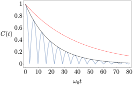
(a)

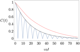
(b)

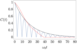
(c)

Figure 6: (Color online) The effect of different instantaneous unitaries applied between the channels in the construction of the perturbed channels of Eq. (40). In each plot we show the CJ concurrence $C(t)$ of the unperturbed amplitude-damping processes ${\Phi}_{0\rightarrow t}$ without interruptions (solid blue line) and its decaying envelope (black dotted line), for $\alpha=5\omega_{0}$ and $\lambda=0.1\omega_{0}$ as in Fig. 4. The temporal behavior of CJ concurrence of the associated perturbed maps (38) for different exemplary unitaries is shown by the red dot-dashed line: a) the unitary is the identity operator, i.e., $\theta=0$; b) $\theta=3.11$ and $\phi=0.5$; c) $\theta=3.11$ and $\phi=1.2$. The identity leads to optimal entanglement preservation (the same result has been verified numerically for other choices of the system parameters). Furthermore, as shown in panel c), some choices of unitary $U$ can lead to the complete and irreversible destruction of entanglement in the state.

References

- [1] A. S. Holevo, Quantum Systems, Channels, Information. A Mathematical Introduction (De Gruyter, Berlin/Boston, 2012).
- [2] M. A. Nielsen and I. L. Chuang, Quantum Computation and Quantum Information (Cambridge: Cambridge University Press, 2010).
- [3] N. Gisin, G. Ribordy, W. Tittel, and H. Zbinden, Rev. Mod. Phys. 74, 145 (2002).
- [4] R. Horodecki, P. Horodecki, M. Horodecki, and K. Horodecki, Rev. Mod. Phys. 81, 865 (2009).
- [5] C. H. Bennett, G. Brassard, S. Popescu, B. Schumacher, J. A. Smolin, and W. K. Wootters, Phys. Rev. Lett. 76, 722 (1996).
- [6] P. W. Shor, Phys. Rev. A 52, R2493 (1995).
- [7] A. M. Steane, Proc. R. Soc. London A 452, 2551 (1996).
- [8] B. M. Terhal, Rev. Mod. Phys. 87, 307 (2015).
- [9] T. Yu, J. H. Eberly, Quantum Inf. Comput. 7, 459-468 (2007).
- [10] P. Zanardi and M. Rasetti, Phys. Rev. Lett. 79, 3306 (1997).
- [11] D. A. Lidar, I. L. Chuang and K. B. Whaley, Phys. Rev. Lett. 81, 2594 (1998).
- [12] L. Viola and S. Lloyd, Phys. Rev. A 58, 2733 (1998).
- [13] L. Viola and E. Knill, Phys. Rev. Lett. 94, 060502 (2005).
- [14] S. Damodarakurup, M. Lucamarini, G. Di Giuseppe, D. Vitali and P. Tombesi, Phys. Rev. Lett. 103, 040502 (2009).
- [15] P. Facchi, S. Tasaki, S. Pascazio, H. Nakazato, A. Tokuse, and D. A. Lidar, Phys. Rev. A 71, 022302 (2005).
- [16] S. Maniscalco, F. Francica, R. L. Zaffino, N. Lo Gullo, and F. Plastina, Phys. Rev. Lett. 100, 090503 (2008).
- [17] A. Orieux, A. D’Arrigo, G. Ferranti, R. Lo Franco, G. Benenti, E. Paladino, G. Falci, F. Sciarrino and P. Mat- aloni, Sci. Rep. 5 8575 (2015).
- [18] A. Cuevas, A. Mari, A. De Pasquale, A. Orieux, M. Massaro, F. Sciarrino, P. Mataloni, and V. Giovannetti Phys. Rev. A 96, 012314 (2017).
- [19] M. Horodecki, P. W. Shor and M. B. Ruskai, Rev. Math. Phys 15, 629 (2003).
- [20] A. S. Holevo, Russian. Math. Surveys 53, 1295 (1998).
- [21] D. D. Chrúscinśki, and A. Kossakowski, Open Syst. Inf. Dyn. 13, 17 (2006).
- [22] D. Gatto, A. De Pasquale and V. Giovannetti, arXiv:1806.07468
- [23] H.-P. Breuer and F. Petruccione, The Theory of Open Quantum Systems (Oxford University Press, Oxford, New York, 2002).
- [24] H.-P. Breuer, E.-M. Laine, J. Piilo and B. Vacchini, Rev. Mod. Phys. 88, 021002 (2016).
- [25] A. Rivas, S. F. Huelga, and M. B. Plenio, Rep. Prog. Phys. 77, 094001 (2014).
- [26] B. Bellomo, R. Lo Franco, and G. Compagno, Phys. Rev. Lett. 99, 160502 (2007).
- [27] L. Mazzola, S. Maniscalco, J. Piilo, K.-A. Suominen, and B. M. Garraway, Phys. Rev. A 79, 042302 (2009).
- [28] A. Rivas, S. F. Huelga, and M. B. Plenio, Phys. Rev. Lett. 105, 050403 (2010).
- [29] B. Bellomo, R. Lo Franco, S. Maniscalco, and G. Compagno, Phys. Rev. A 78, 060302(R) (2008).
- [30] A. De Pasquale and V. Giovannetti, Phys. Rev. A 86, 052302 (2012).
- [31] A. De Pasquale, A. Mari, A. Porzio, and V. Giovannetti, Phys. Rev. A 87, 062307 (2013).
- [32] A. Cuevas, et al., Phys. Rev. A 96, 022322 (2017).
- [33] D. Buono, et al. Eprint arXiv:1312.2763 [quant-ph].
- [34] G. Lindblad, Commun. Math. Phys. 48, 119-130 (1976).
- [35] V. Gorini, A. Kossakowski, and E. C. Sudarshan, J. Math. Phys. 17, 821 (1976).
- [36] B. Bylicka, M. Johansson, and A. Acin, Phys. Rev. Lett. 118, 120501 (2017).
- [37] H.-P. Breuer, E.-M. Laine, and J. Piilo, Phys. Rev. Lett. 103, 210401 (2009).
- [38] M.-D Choi, Linear Alg. and Its Appl. 10, 285 (1975).
- [39] A. Jamiolkowski, Rep. Mat. Phys. 3, 275 (1972).
- [40] W. K. Wootters, Phys. Rev. Lett. 80, 2245 (1998).
- [41] D. D. Chrúscinśki, and S. Maniscalco, Phys. Rev. Lett. 112, 120404 (2014).
- [42] C. King, IEEE Trans. Inf. Theory, vol. 49, 221 (2003).
- [43] P. Haikka, T. H. Johnson, and S. Maniscalco, Phys. Rev. A 87, 010103(R) (2013).
- [44] P. Haikka and S. Maniscalco, Phys. Rev. A 81, 052103 (2010).
- [45] P. Facchi and S. Pascazio, Progress in Optics, edited by E. Wolf (Elsevier, Amsterdam, 2001), Vol. 42, Chapter 3, pp. 147-218.