Casimir force for magnetodielectric media

Abstract

Boyer showed that a perfect electrically conducting slab repels a perfect magnetically conducting slab, in contrast to the attractive Casimir force between two identical perfect electrically or magnetically conducting slabs. To gain insight for the difference between the Boyer force and the Casimir force, we present the derivation of the Boyer force using the stress tensor method and then using the method of variation in dielectric. The Green dyadic, in terms of electric and magnetic Green’s functions, is presented for an electric medium filling half of space and another magnetic medium filling another half of space such that the two half-spaces are parallel and separated by a distance $a$. We make the observation that the spectral distribution of scattering in a Boyer cavity is that of Fermi-Dirac type, while the spectral distribution of scattering in a Casimir cavity is that of Bose-Einstein type. Based on this observation we conclude that the difference between the Boyer force and the Casimir force is governed by the statistics of the possible scattering in the respective cavities.

I Introduction

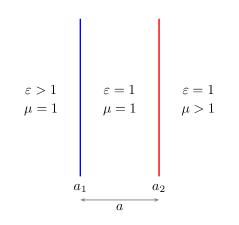
Consider the Boyer configuration of parallel slabs, consisting of two parallel semi-infinitely thick plates, separated by a vacuum gap $a$. Let the left plate be situated at $z=a_{1}$, the right plate at $z=a_{2}$, so that $a=a_{2}-a_{1}$, see Fig. 1. Let the right plate be purely paramagnetic ($\mu>1,\varepsilon=1$), and the left plate purely dielectric ($\varepsilon>1,\mu=1$). The Boyer configuration of slabs should be contrasted with the Casimir configuration of parallel slabs in Fig. 2. We shall be interested in the pressure, called $P$ here, between the slabs. For simplicity we limit ourselves to zero temperature. (General treatises on the Casimir effect can be found in Refs. Milton (2001); Bordag et al. (2009); Dalvit et al. (2011).)

Stimulated by a suggestion from Casimir, Boyer Boyer (1974) made an explicit calculation of the force between an infinitely permeable magnetic medium ($\mu\rightarrow\infty$) and a perfect conductor ($\varepsilon\rightarrow\infty$). The interaction energy per unit area was found to be

$$U=\frac{7}{8}\,\frac{\pi^{2}\hbar c}{720a^{3}},$$ (1)

which corresponds to a repulsive pressure

$$P=\frac{7}{8}\,|P_{0}|,$$ (2)

where

$$P_{0}=-\frac{\pi^{2}\hbar c}{240a^{4}}$$ (3)

is the attractive force between two perfectly conducting plates. As explained by Boyer, this is related to the fact that while an electrically polarizable particle is attracted to a conducting wall, a magnetically polarizable particle is repelled by it (the latter case being analogous to the hydrodynamic flow from a point or line source outside an impenetrable plane).

From the standpoint of optical physics this result is however rather perplexing. Consider for definiteness the electromagnetic force density f on the boundary layer in the left plate; this force is purely electric, and is calculated from the divergence of Maxwell’s stress tensor to be

$${\bf f}=-\frac{1}{2}E^{2}{\bm{\nabla}}\varepsilon.$$ (4)

In classical physics this force always acts towards the optically thinner medium, that is, towards the vacuum region for the plate in consideration. One can observe that the direction of this force given by the direction of ${\bm{\nabla}}\varepsilon$ is independent of the magnetic properties of the right plate. The direction is determined by the gradient of the dielectric permittivity $\varepsilon$ only. Even if the magnetic properties of the right plate should change, the electric field ${\bf E}$ on the left plate would change, but the direction of this force would be just the same.

The magnitude of the surface pressure $P$ can be found by integrating the normal component $f_{z}$ across the boundary located at $z=a_{1}$. Now there are numerous cases in optics showing the reality of the expression in Eq. (4). For example, the classic experiment of Ashkin and Dziedzic Ashkin and Dziedzic (1973), demonstrating the outward bulge of a water surface illuminated by a radiation beam coming from above, is of this sort, as is the newer version of this experiment due to Astrath et al. Astrath et al. (2014) (a review of some radiation pressure experiments of this sort can be found in Ref. Brevik (2017)). Also, the recent pressure experiment of Kundu et al. Kundu et al. (2017), showing the deflection of a graphene sheet upon laser illumination, belongs to the same category. In all these cases, the force was found to act in the direction of the optically thinner medium, in accordance with the expression in Eq. (4).

Figure 1: Boyer configuration of parallel slabs.

If one leaves the regime of classical physics and moves on to the quantum mechanical calculation of the Casimir pressure, one finds analogous results as long as both plates, separated by a vacuum gap, are either purely dielectric or purely magnetic. This pressure is conventionally calculated by taking the difference between the $zz$ components of Maxwell’s stress tensor on the two sides, making use of the fluctuation-dissipation theorem when constructing the two-point functions for the electric and magnetic fields. Again, the pressure is found to be attractive, in accordance with Eq. (4).

Now return to the magnetodielectric case considered by Boyer. At first glance one would think that the repulsiveness of the force as mentioned above is in direct conflict with Eq. (4). What is the physical reason for this? Formally, the situation would mean that one has to reverse the sign of the quadratic quantity $E^{2}$ in Eq. (4). In view of this bizarre situation, one would think that a revisit of the fundamental assumptions behind electromagnetic theory in matter is desirable. That was one of the motivations behind the present paper.

We first present the Green function formalism in a general way in Sec. II, and provide explicit solutions for the Green dyadic in Sec. III, where the two plates are each allowed to possess arbitrary, even frequency-dependent, values of $\mu$ and $\varepsilon$, and calculate the surface force formally in Sec. IV. Thereafter we specialize to the Boyer case. We make the observation that the spectral distribution of scattering in a Boyer cavity is that of Fermi-Dirac type, while the spectral distribution of scattering in a Casimir cavity is that of Bose-Einstein type. Based on this observation we suggest that the difference between the Boyer force and the Casimir force is statistics of the possible scattering in the respective cavities.

Next, we inquire if the Boyer force is sensitive to a cutoff in the frequency response of permeability $\mu$. Calculations of the Boyer force have usually assumed $\mu$ to be a constant for all frequencies. It is easy to see that this is a over-simplified model that violates one of the fundamentals of macroscopic theory (cf. also the discussion in Ref. Landau and Lifshitz (1984)): Start from the “microscopic” Maxwell equation (here in Heaviside-Lorentz units)

$${\bm{\nabla}}\times{\bf h}=\rho{\bf v}+\frac{\partial{\bf e}}{\partial t},$$ (5)

where $\rho\bf{v}$ is the local current density and ${\bf h}$ and ${\bf e}$ are the local magnetic and electric fields. Space averaging gives $\overline{\bf h}={\bf B}$ with ${\bf B}$ the magnetic induction, and $\overline{\bf e}={\bf E}$ with ${\bf E}$ the macroscopic electric field. Thus

$${\bm{\nabla}}\times{\bf B}=\overline{\rho{\bf v}}+\frac{\partial{\bf E}}{\partial t}.$$ (6)

Subtracting the Maxwell equation ${\bm{\nabla}}\times{\bf H}=\partial{\bf D}/\partial t$ we get

$$\overline{\rho{\bf v}}={\bm{\nabla}}\times{\bf M}+\frac{\partial{\bf P}}{\partial t},$$ (7)

with ${\bf M}={\bf B}-{\bf H}$ and ${\bf P}={\bf D}-{\bf E}$.

Figure 2: Casimir configuration of parallel slabs.

Consider now the general definition of the magnetic moment ${\bf m}$ of a body,

$${\bf m}=\frac{1}{2}\int{\bf r}\times\overline{\rho{\bf v}}\,dV.$$ (8)

This can be compared with the expression

$$\frac{1}{2}\int{\bf r}\times({\bm{\nabla}}\times{\bf M})\,dV=\int{\bf M}\,dV,$$ (9)

which is derived using vector manipulations observing that ${\bf M}=0$ in the vacuum region outside the body. Since ${\bf m}=\int{\bf M}\,dV$ it follows that we can put $\overline{\rho{\bf v}}$ equal to ${\bm{\nabla}}\times{\bf M}$. Comparing with Eq. (7) we conclude that the consistency of macroscopic electrodynamics depends on the possibility to neglect the $\partial{\bf P}/\partial t$ term. This can be made concrete further by assuming that the body of linear size $l$ is exposed to an electromagnetic wave of frequency $\omega$. We shall insert speed of light $c$, momentarily, in expressions in this section for the benefit of the reader. Order of magnitude estimates give $\partial P/\partial t\sim\omega E\sim\omega^{2}lH/c$ (the relationship $E\sim\omega lH/c$ used in the last estimate coming from the equation ${\bm{\nabla}}\times{\bf E}=-\partial{\bf B}/\partial t$ and $E\sim H$). The first term on the right hand side of Eq. (7) is ${\bm{\nabla}}\times{\bf M}=\chi{\bm{\nabla}}\times{\bf H}$ where $\chi$ is the susceptibility, and is estimated to be of order $c\chi H/l$. Thus, our consistency condition reduces to

$$l^{2}\ll\chi c^{2}/\omega^{2};$$ (10)

an inequality already given in Ref. Landau and Lifshitz (1984). It is easily seen that the inequality in Eq. (10) is broken already at frequencies $\omega$ much less than optical frequencies. And that is confirmed by experiments also. For instance, for ferrite with $\mu\approx 600$ the maximum of the frequency $\omega/2\pi$ is reported to lie in the region 100 kHz to 1 MHz NPL (2005). The assumption about a very large and constant permeability as used in the Boyer calculation is obviously unphysical.

In Sec. V we take the magnetic dispersion into account in a crude way, by assuming $\mu$ to be constant up to a critical value $\omega=\omega_{c}$. For higher frequencies we set $\mu=1$. Thus

$$\mu(\omega)=\begin{cases}\mu,&\omega<\omega_{c},\\ 1,&\omega>\omega_{c}.\end{cases}$$ (11)

As one might expect, we do not find a reversal of the sign of the force in this way; the force still comes out repulsive. So the basic problem alluded to at the beginning, is not solved. However, an important physical result of the calculation is that the force turns out to be immeasurably small, when realistic input data for $\omega_{c}$ are inserted. This makes it evident why the repulsive force has never been measured. It may finally be mentioned that we will keep $\varepsilon$ constant, at all frequencies. There is no comparably strong limit to the permittivity as it is to the permeability.

In Sec. VI we consider the Boyer problem from a statistical mechanical point of view, introducing a model where the two media are represented by harmonic oscillators 1 and 2, interacting with each other via a third oscillator 3. In this way a mechanical analogue to the conventional TE and TM modes in electromagnetism is obtained. We find that the quantum mechanical transition from the TM to the TE mode, implying that oscillator 3 interacts with oscillators 1 and 2 via canonical momenta instead of positions, is an important point. In this way the statistical mechanical analysis helps us to elucidate the problem.

II Maxwell’s equations

In Heaviside-Lorentz units the monochromatic components of Maxwell’s equations, proportional to $\exp(-i\omega t)$, in the absence of net charges and currents, and in presence of dielectric and magnetic materials with boundaries, are

$${\bm{\nabla}}\times{\bf E} =i\omega{\bf B},$$ (12a)

$$-{\bm{\nabla}}\times{\bf H} =i\omega({\bf D}+{\bf P}).$$ (12b)

These equations imply ${\bm{\nabla}}\cdot{\bf B}=0$ and ${\bm{\nabla}}\cdot({\bf D}+{\bf P})=0$. Here ${\bf P}$ is an external source of polarization, in addition to the polarization of the material in response to the fields ${\bf E}$ and ${\bf H}$. The external source ${\bf P}$ serves as a convenient mathematical tool, and is set to zero in the end. In the following we neglect non-linear responses and assume that the fields ${\bf D}$ and ${\bf B}$ respond linearly to the electric and magnetic fields ${\bf E}$ and ${\bf H}$:

$${\bf D}({\bf r},\omega) ={\bm{\varepsilon}}({\bf r};\omega)\cdot{\bf E}({\bf r},\omega),$$ (13a)

$${\bf B}({\bf r},\omega) ={\bm{\mu}}({\bf r};\omega)\cdot{\bf H}({\bf r},\omega).$$ (13b)

Using Eq. (12a) in Eq. (12b) we construct the following differential equation for the electric field,

$$\left[\frac{1}{\omega^{2}}{\bm{\nabla}}\times{\bm{\mu}}^{-1}\cdot{\bm{\nabla}}\times\;-{\bf 1}-{\bm{\chi}}\right]\cdot{\bf E}({\bf r},\omega)={\bf P}({\bf r},\omega),$$ (14)

where

$${\bm{\chi}}({\bf r};\omega)={\bm{\varepsilon}}({\bf r};\omega)-{\bf 1}.$$ (15)

The differential equation for the Green’s dyadic ${\bm{\Gamma}}({\bf r},{\bf r}^{\prime};\omega)$ is guided by Eq. (14),

$$\left[\frac{1}{\omega^{2}}{\bm{\nabla}}\times{\bm{\mu}}^{-1}\cdot{\bm{\nabla}}\times\;-{\bf 1}-{\bm{\chi}}\right]\cdot{\bm{\Gamma}}({\bf r},{\bf r}^{\prime};\omega)={\bf 1}\delta^{(3)}({\bf r}-{\bf r}^{\prime}).$$ (16)

It defines the relation between the electric field and the polarization source,

$${\bf E}({\bf r};\omega)=\int d^{3}r^{\prime}{\bm{\Gamma}}({\bf r},{\bf r}^{\prime};\omega)\cdot{\bf P}({\bf r}^{\prime};\omega).$$ (17)

The corresponding dyadic for vacuum, obtained by setting ${\bm{\chi}}=0$, is called the free Green’s dyadic and satisfies the equation

$$\left[\frac{1}{\omega^{2}}{\bm{\nabla}}\times{\bm{\mu}}^{-1}\cdot{\bm{\nabla}}\times\;-{\bf 1}\right]\cdot{\bm{\Gamma}}_{0}({\bf r},{\bf r}^{\prime};\omega)={\bf 1}\delta^{(3)}({\bf r}-{\bf r}^{\prime}).$$ (18)

We can also define the relation between the magnetic field and the polarization source,

$${\bf H}({\bf r};\omega)=\int d^{3}r^{\prime}{\bm{\Phi}}({\bf r},{\bf r}^{\prime};\omega)\cdot{\bf P}({\bf r}^{\prime};\omega).$$ (19)

II.1 Quantum electrodynamics

The Green dyadics gives the correlation between the fields and sources, as per Eqs. (17) and (19),

$$\frac{\delta{\bf E}({\bf r};\omega)}{\delta{\bf P}({\bf r}^{\prime};\omega)} ={\bm{\Gamma}}({\bf r},{\bf r}^{\prime};\omega),$$ (20a)

$$\frac{\delta{\bf H}({\bf r};\omega)}{\delta{\bf P}({\bf r}^{\prime};\omega)} ={\bm{\Phi}}({\bf r},{\bf r}^{\prime};\omega).$$ (20b)

In quantum electrodynamics the Green dyadics also serve as correlations between the fields at two different points in space, which are stated as

$$\frac{1}{\tau}\langle{\bf E}({\bf r};-\omega){\bf E}({\bf r}^{\prime};\omega)\rangle =\frac{1}{i}{\bm{\Gamma}}({\bf r},{\bf r}^{\prime};\omega),$$ (21a)

$$\frac{1}{\tau}\langle{\bf H}({\bf r};-\omega){\bf H}({\bf r}^{\prime};\omega)\rangle =\frac{1}{i}{\bm{\Gamma}}({\bf r},{\bf r}^{\prime};\omega)\Big{|}_{E\leftrightarrow H,\varepsilon\leftrightarrow\mu},$$ (21b)

$$\frac{1}{\tau}\langle{\bf H}({\bf r};-\omega){\bf E}({\bf r}^{\prime};\omega)\rangle =\frac{1}{i}{\bm{\Phi}}({\bf r},{\bf r}^{\prime};\omega)$$ (21c)

$$\frac{1}{\tau}\langle{\bf E}({\bf r};-\omega){\bf H}({\bf r}^{\prime};\omega)\rangle^{*} =\frac{1}{i}{\bm{\Phi}}({\bf r},{\bf r}^{\prime};\omega),$$ (21d)

where $\tau$ is the average (infinite) time for which the system is observed.

III Green’s dyadic

For planar geometry, using translational symmetry in the plane, we can define the Fourier transformations

$${\bm{\Gamma}}({\bf r},{\bf r}^{\prime};\omega) =\int\frac{d^{2}k_{\perp}}{(2\pi)^{2}}\,e^{i{\bf k}_{\perp}\cdot({\bf r}-{\bf r}^{\prime})_{\perp}}{\bm{\gamma}}(z,z^{\prime};k_{\perp},\omega),$$ (22a)

$${\bm{\Phi}}({\bf r},{\bf r}^{\prime};\omega) =\int\frac{d^{2}k_{\perp}}{(2\pi)^{2}}\,e^{i{\bf k}_{\perp}\cdot({\bf r}-{\bf r}^{\prime})_{\perp}}{\bm{\phi}}(z,z^{\prime};k_{\perp},\omega).$$ (22b)

The reduced Green’s dyadics can be expressed in the form

$${\bm{\gamma}}=\left[\begin{array}[]{ccc}\frac{1}{\varepsilon^{\perp}(z)}\frac{\partial}{\partial z}\frac{1}{\varepsilon^{\perp}(z^{\prime})}\frac{\partial}{\partial z^{\prime}}g^{H}&0&\frac{1}{\varepsilon^{\perp}(z)}\frac{\partial}{\partial z}\frac{ik_{\perp}}{\varepsilon^{||}(z^{\prime})}g^{H}\\[5.69054pt] 0&\omega^{2}g^{E}&0\\[5.69054pt] -\frac{ik_{\perp}}{\varepsilon^{||}(z)}\frac{1}{\varepsilon^{\perp}(z^{\prime})}\frac{\partial}{\partial z^{\prime}}g^{H}&0&-\frac{ik_{\perp}}{\varepsilon^{||}(z)}\frac{ik_{\perp}}{\varepsilon^{||}(z^{\prime})}g^{H}\end{array}\right].$$ (23)

Here we have omitted the term

$$-\delta(z-z^{\prime})\left[\begin{array}[]{llr}\frac{1}{\varepsilon^{\perp}(z)}&0&0\\ 0&0&0\\ 0&0&\frac{1}{\varepsilon^{||}(z)}\end{array}\right]$$ (24)

that contains a $\delta$-function and thus never contributes to interaction energies between two bodies unless they are overlapping, and

$${\bm{\phi}}=i\omega\left[\begin{array}[]{ccc}0&\frac{1}{\mu^{\perp}(z)}\frac{\partial}{\partial z}g^{E}&0\\[5.69054pt] \frac{1}{\varepsilon^{\perp}(z^{\prime})}\frac{\partial}{\partial z^{\prime}}g^{H}&0&\frac{ik_{\perp}}{\varepsilon^{||}(z^{\prime})}g^{H}\\[5.69054pt] 0&-\frac{ik_{\perp}}{\mu^{||}(z)}g^{E}&0\end{array}\right].$$ (25)

Here the magnetic (TM mode) Green’s function $g^{H}(z,z^{\prime})$, and the electric (TE mode) Green’s function $g^{E}(z,z^{\prime})$, are defined using the differential equations

$$\left[-\frac{\partial}{\partial z}\frac{1}{\varepsilon^{\perp}(z)}\frac{\partial}{\partial z}+\frac{k_{\perp}^{2}}{\varepsilon^{||}(z)}-\omega^{2}\mu^{\perp}(z)\right]g^{H} = \delta(z-z^{\prime}),\hskip 25.60747pt$$ (26a)

$$\left[-\frac{\partial}{\partial z}\frac{1}{\mu^{\perp}(z)}\frac{\partial}{\partial z}+\frac{k_{\perp}^{2}}{\mu^{||}(z)}-\omega^{2}\varepsilon^{\perp}(z)\right]g^{E} = \delta(z-z^{\prime}),$$ (26b)

where $\varepsilon=\text{diag}(\varepsilon^{\perp},\varepsilon^{\perp},\varepsilon^{||})$ is the permittivity tensor and $\mu=\text{diag}(\mu^{\perp},\mu^{\perp},\mu^{||})$ is the permeability tensor Parashar et al. (2012).

III.1 Electric Green’s function for Boyer configuration

Figure 3: Labels for the regions in the $z$-$z^{\prime}$ space, used for specifying the Green function.

For the Boyer configuration of slabs in Fig. 1 with isotropic permittivity $\varepsilon$ and permeability $\mu$ we have the differential equation for the electric Green’s function

$$\left[-\frac{\partial}{\partial z}\frac{1}{\mu(z)}\frac{\partial}{\partial z}+\frac{k_{\perp}^{2}}{\mu(z)}-\omega^{2}\varepsilon(z)\right]g^{E}(z,z^{\prime})=\delta(z-z^{\prime}),$$ (27)

where

$$\varepsilon(z) =1+(\varepsilon-1)\,\theta(a_{1}-z),$$ (28a)

$$\mu(z) =1+(\mu-1)\,\theta(z-a_{2}),$$ (28b)

with boundary conditions

$$g^{E}(z,z^{\prime})\Big{|}^{a_{i}+\delta}_{a_{i}-\delta} = 0,$$ (29a)

$$\left\{\frac{1}{\mu(z)}\frac{\partial}{\partial z}g^{E}(z,z^{\prime})\right\}\bigg{|}^{a_{i}+\delta}_{a_{i}-\delta} = 0.$$ (29b)

In terms of shorthand notations for typesetting

$$\kappa=\sqrt{k_{\perp}^{2}+\zeta^{2}},$$ (30)

and

$$\kappa_{\varepsilon}=\sqrt{k_{\perp}^{2}+\zeta^{2}\varepsilon},\qquad\kappa_{\mu}=\sqrt{k_{\perp}^{2}+\zeta^{2}\mu},$$ (31)

and

$$\bar{\kappa}_{\varepsilon}=\frac{\kappa_{\varepsilon}}{\varepsilon},\qquad\qquad\bar{\kappa}_{\mu}=\frac{\kappa_{\mu}}{\mu},$$ (32)

and

$$r_{\varepsilon}=r_{1}^{E} =\frac{\kappa_{\varepsilon}-\kappa}{\kappa_{\varepsilon}+\kappa}, r_{2}^{E} =0,$$ (33a)

$$r_{1}^{H} =0, r_{2}^{H} =\frac{\bar{\kappa}_{\mu}-\kappa}{\bar{\kappa}_{\mu}+\kappa}=r_{\mu},$$ (33b)

and

$$\Delta^{E} =1-r_{\varepsilon}\bar{r}_{\mu}e^{-2\kappa a},$$ (34a)

$$\Delta^{H} =1-\bar{r}_{\varepsilon}r_{\mu}e^{-2\kappa a},$$ (34b)

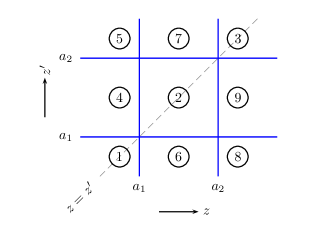
where $\bar{r}_{\varepsilon}$ is obtained by replacing $\kappa_{\varepsilon}\to\bar{\kappa}_{\varepsilon}$ in $r_{\varepsilon}$, and, similarly, $\bar{r}_{\mu}$ is obtained by replacing $\kappa_{\mu}\to\bar{\kappa}_{\mu}$ in $r_{\mu}$. In the following the label in the subscript represents the region in Fig. 3 in which the variables $z$ and $z^{\prime}$ reside. The solution for the electric Green’s function is,

$$g^{E}_{\rput(2.84526pt,0.0pt){\scriptstyle{1}}{\psset{linewidth=0.2pt}\pscircle(2.84526pt,0.28452pt){3.69885pt}}}(z,z^{\prime}) =\frac{1}{2\kappa_{\varepsilon}}e^{-\kappa_{\varepsilon}|z-z^{\prime}|}+\frac{1}{2\kappa_{\varepsilon}}\frac{1}{\Delta^{E}}\Big{[}r_{\varepsilon}-\bar{r}_{\mu}e^{-2\kappa a}\Big{]}e^{-\kappa_{\varepsilon}|a_{1}-z|}e^{-\kappa_{\varepsilon}|a_{1}-z^{\prime}|}, z,z^{\prime}<a_{1}<a_{2},$$ (35a)

$$g^{E}_{\rput(2.84526pt,0.0pt){\scriptstyle{4}}{\psset{linewidth=0.2pt}\pscircle(2.84526pt,0.28452pt){3.69885pt}}}(z,z^{\prime}) =\frac{1}{\kappa_{\varepsilon}+\kappa}\frac{1}{\Delta^{E}}e^{-\kappa_{\varepsilon}|a_{1}-z|}e^{-\kappa|z^{\prime}-a_{1}|}-\frac{1}{\kappa_{\varepsilon}+\kappa}\frac{1}{\Delta^{E}}\Big{[}\bar{r}_{\mu}e^{-\kappa a}\Big{]}e^{-\kappa_{\varepsilon}|a_{1}-z|}e^{-\kappa|a_{2}-z^{\prime}|}, z<a_{1}<z^{\prime}<a_{2},$$ (35b)

$$g^{E}_{\rput(2.84526pt,0.0pt){\scriptstyle{5}}{\psset{linewidth=0.2pt}\pscircle(2.84526pt,0.28452pt){3.69885pt}}}(z,z^{\prime}) =\frac{1}{2\kappa}\frac{1}{\Delta^{E}}\Big{[}\frac{2\kappa}{\kappa_{\varepsilon}+\kappa}\frac{2\kappa}{\bar{\kappa}_{\mu}+\kappa}e^{-\kappa a}\Big{]}e^{-\kappa_{\varepsilon}|a_{1}-z|}e^{-\kappa_{\mu}|z^{\prime}-a_{2}|}, z<a_{1}<a_{2}<z^{\prime},$$ (35c)

and

$$g^{E}_{\rput(2.84526pt,0.0pt){\scriptstyle{6}}{\psset{linewidth=0.2pt}\pscircle(2.84526pt,0.28452pt){3.69885pt}}}(z,z^{\prime}) =\frac{1}{\kappa_{\varepsilon}+\kappa}\frac{1}{\Delta^{E}}e^{-\kappa|z-a_{1}|}e^{-\kappa_{\varepsilon}|a_{1}-z^{\prime}|}-\frac{1}{\kappa_{\varepsilon}+\kappa}\frac{1}{\Delta^{E}}\Big{[}\bar{r}_{\mu}e^{-\kappa a}\Big{]}e^{-\kappa|a_{2}-z|}e^{-\kappa_{\varepsilon}|a_{1}-z^{\prime}|},\hskip 14.22636ptz^{\prime}<a_{1}<z<a_{2},$$ (36a)

$$g^{E}_{\rput(2.84526pt,0.0pt){\scriptstyle{2}}{\psset{linewidth=0.2pt}\pscircle(2.84526pt,0.28452pt){3.69885pt}}}(z,z^{\prime}) =\frac{1}{2\kappa}e^{-\kappa|z-z^{\prime}|}-\frac{1}{2\kappa}\frac{1}{\Delta^{E}}\Big{[}r_{\varepsilon}\Big{]}e^{-\kappa|z-a_{1}|}e^{-\kappa|z^{\prime}-a_{1}|}+\frac{1}{2\kappa}\frac{1}{\Delta^{E}}\Big{[}r_{\varepsilon}\bar{r}_{\mu}e^{-\kappa a}\Big{]}e^{-\kappa|z-a_{1}|}e^{-\kappa|a_{2}-z^{\prime}|}$$

$$\hskip 11.38109pt+\frac{1}{2\kappa}\frac{1}{\Delta^{E}}\Big{[}\bar{r}_{\mu}r_{\varepsilon}e^{-\kappa a}\Big{]}e^{-\kappa|a_{2}-z|}e^{-\kappa|z^{\prime}-a_{1}|}-\frac{1}{2\kappa}\frac{1}{\Delta^{E}}\Big{[}\bar{r}_{\mu}\Big{]}e^{-\kappa|a_{2}-z|}e^{-\kappa|a_{2}-z^{\prime}|},\hskip 19.91692pta_{1}<z^{\prime},z<a_{2},$$ (36b)

$$g^{E}_{\rput(2.84526pt,0.0pt){\scriptstyle{7}}{\psset{linewidth=0.2pt}\pscircle(2.84526pt,0.28452pt){3.69885pt}}}(z,z^{\prime}) =\frac{1}{\bar{\kappa}_{\mu}+\kappa}\frac{1}{\Delta^{E}}e^{-\kappa|a_{2}-z|}e^{-\kappa_{\mu}|z^{\prime}-a_{2}|}-\frac{1}{\bar{\kappa}_{\mu}+\kappa}\frac{1}{\Delta^{E}}\Big{[}r_{\varepsilon}e^{-\kappa a}\Big{]}e^{-\kappa|z-a_{1}|}e^{-\kappa_{\mu}|z^{\prime}-a_{2}|},\hskip 14.22636pta_{1}<z<a_{2}<z^{\prime},$$ (36c)

and

$$g^{E}_{\rput(2.84526pt,0.0pt){\scriptstyle{8}}{\psset{linewidth=0.2pt}\pscircle(2.84526pt,0.28452pt){3.69885pt}}}(z,z^{\prime}) =\frac{1}{2\kappa}\frac{1}{\Delta^{E}}\Big{[}\frac{2\kappa}{\kappa_{\varepsilon}+\kappa}\frac{2\kappa}{\bar{\kappa}_{\mu}+\kappa}e^{-\kappa a}\Big{]}e^{-\kappa_{\mu}|z-a_{2}|}e^{-\kappa_{\varepsilon}|a_{1}-z^{\prime}|}, z^{\prime}<a_{1}<a_{2}<z,$$ (37a)

$$g^{E}_{\rput(2.84526pt,0.0pt){\scriptstyle{9}}{\psset{linewidth=0.2pt}\pscircle(2.84526pt,0.28452pt){3.69885pt}}}(z,z^{\prime}) =\frac{1}{\bar{\kappa}_{\mu}+\kappa}\frac{1}{\Delta^{E}}e^{-\kappa_{\mu}|z-a_{2}|}e^{-\kappa|a_{2}-z^{\prime}|}-\frac{1}{\bar{\kappa}_{\mu}+\kappa}\frac{1}{\Delta^{E}}\Big{[}r_{\varepsilon}e^{-\kappa a}\Big{]}e^{-\kappa_{\mu}|z-a_{2}|}e^{-\kappa|z^{\prime}-a_{1}|}, a_{1}<z^{\prime}<a_{2}<z,$$ (37b)

$$g^{E}_{\rput(2.84526pt,0.0pt){\scriptstyle{3}}{\psset{linewidth=0.2pt}\pscircle(2.84526pt,0.28452pt){3.69885pt}}}(z,z^{\prime}) =\frac{1}{2\bar{\kappa}_{\mu}}e^{-\kappa_{\mu}|z-z^{\prime}|}+\frac{1}{2\bar{\kappa}_{\mu}}\frac{1}{\Delta^{E}}\Big{[}\bar{r}_{\mu}-r_{\varepsilon}e^{-2\kappa a}\Big{]}e^{-\kappa_{\mu}|z-a_{2}|}e^{-\kappa_{\mu}|z^{\prime}-a_{2}|}, a_{1}<a_{2}<z^{\prime},z.$$ (37c)

III.2 Magnetic Green’s function for Boyer configuration

For the Boyer configuration of slabs in Fig. 3 the magnetic Green’s function has the differential equation

$$\left[-\frac{\partial}{\partial z}\frac{1}{\varepsilon(z)}\frac{\partial}{\partial z}+\frac{k_{\perp}^{2}}{\varepsilon(z)}-\omega^{2}\mu(z)\right]g^{H}(z,z^{\prime})=\delta(z-z^{\prime}),$$ (38)

with boundary conditions

$$g^{H}(z,z^{\prime})\Big{|}^{a_{i}+\delta}_{a_{i}-\delta} = 0,$$ (39a)

$$\left\{\frac{1}{\varepsilon(z)}\frac{\partial}{\partial z}g^{H}(z,z^{\prime})\right\}\bigg{|}^{a_{i}+\delta}_{a_{i}-\delta} = 0.$$ (39b)

The solution for the magnetic Green’s function is obtained from the electric Green’s function by replacing $\kappa_{\varepsilon}\to\bar{\kappa}_{\varepsilon}$ and $\bar{\kappa}_{\mu}\to\kappa_{\mu}$ everywhere, except in the exponentials. This leads to the replacements, $r_{\varepsilon}\to\bar{r}_{\varepsilon}$, $\bar{r}_{\mu}\to r_{\mu}$, and $\Delta^{E}\to\Delta^{H}$.

III.3 Perfect electric and magnetic conductors

In the limit $\varepsilon\to\infty$ and $\mu\to\infty$, when the region $z<a_{1}$ is a perfectly conducting electric medium and the region $z>a_{1}$ is a perfectly conducting magnetic material, we observe that the region corresponding to $a_{1}<z,z^{\prime}<a_{2}$ in Fig. 1 is the only relevant region in the discussion as the fields vanish inside the two perfectly conducting media. Thus, we have

$$\Delta_{\textrm{PC}}=1+e^{-2\kappa a}.$$ (40)

In this case, the explicit form for the Green functions can be conveniently expressed as

$$g^{E}(z,z^{\prime}) = \frac{1}{\kappa}\frac{\sinh\kappa(z_{<}-a_{1})\cosh\kappa(z_{>}-a_{2})}{\cosh\kappa a},\hskip 31.29802pt$$ (41a)

$$g^{H}(z,z^{\prime}) = -\frac{1}{\kappa}\frac{\cosh\kappa(z_{<}-a_{1})\sinh\kappa(z_{>}-a_{2})}{\cosh\kappa a},$$ (41b)

which is evaluated in region  . Here $z_{<}=\text{Min}(z,z^{\prime})$ and $z_{>}=\text{Max}(z,z^{\prime})$. We make the observation that, on the boundaries of the perfectly conducting slabs at $z=a_{1}$ and $z=a_{2}$ of the Boyer configuration we have

$$g^{E}(a_{1},a_{2}) =0, g^{E}(a_{2},a_{2}) =\frac{\tanh\kappa a}{\kappa},$$ (42a)

$$g^{E}(a_{1},a_{1}) =0, g^{E}(a_{2},a_{1}) =\frac{\sinh\kappa a}{\kappa},$$ (42b)

and

$$g^{H}(a_{1},a_{2}) =0, g^{H}(a_{2},a_{2}) =0,$$ (43a)

$$g^{H}(a_{1},a_{1}) =\frac{\tanh\kappa a}{\kappa}, g^{H}(a_{2},a_{1}) =\frac{\sinh\kappa a}{\kappa}.$$ (43b)

We further make the observation that

$$\frac{\partial}{\partial z}\frac{\partial}{\partial z^{\prime}}g^{E}(z,z^{\prime}) = -\kappa^{2}g^{H}(z,z^{\prime}),$$ (44a)

$$\frac{\partial}{\partial z}\frac{\partial}{\partial z^{\prime}}g^{H}(z,z^{\prime}) = -\kappa^{2}g^{E}(z,z^{\prime}),$$ (44b)

such that

$$\frac{\partial}{\partial z}\frac{\partial}{\partial z^{\prime}}\Big{[}g^{E}(z,z^{\prime})+g^{H}(z,z^{\prime})\Big{]}\bigg{|}_{z=a_{1},z^{\prime}=a_{1}}\hskip 42.67912pt$$

$$=-\kappa^{2}\Big{[}g^{E}(z,z^{\prime})+g^{H}(z,z^{\prime})\Big{]},\hskip 28.45274pt$$ (45)

and

$$g^{E}(a_{1},a_{1})+g^{H}(a_{1},a_{1})=\frac{\tanh\kappa a}{\kappa}.$$ (46)

IV Strong coupling: Boyer’s result

For slowly varying fields, and assuming that the dissipation in the system is negligible, the statement of conservation of momentum density,

$$\rho{\bf E}+\rho{\bf v}\times{\bf B}+\frac{\partial{\bf G}}{\partial t}+{\bm{\nabla}}\cdot{\bf T}-\frac{1}{2}E^{2}{\bm{\nabla}}\varepsilon-\frac{1}{2}H^{2}{\bm{\nabla}}\mu=0,$$ (47)

can be derived starting from the Maxwell equations Parashar et al. (2018), where

$${\bf G}={\bf D}\times{\bf B}$$ (48)

is the momentum density of the electromagnetic field and

$${\bf T}={\bf 1}\frac{1}{2}({\bf D}\cdot{\bf E}+{\bf B}\cdot{\bf H})-({\bf D}{\bf E}+{\bf B}{\bf H})$$ (49)

is the stress tensor or the flux of the momentum density of the electromagnetic field. Each term in Eq. (47) is interpreted as a force when it is integrated over a volume $V$. The first two terms in Eq. (47), together, contribute to the Lorentz force acting on the charges inside volume $V$,

$${\bf f}_{\text{Lor}}=\rho{\bf E}+\rho{\bf v}\times{\bf B},$$ (50)

where $\rho$ is the density of charge and ${\bf v}$ is the velocity of charges that contributes to current density $\rho{\bf v}$. The Lorentz force is zero for a neutral medium. The third term in Eq. (47), when integrated over volume $V$, is the measure of the rate of change of electromagnetic momentum inside the volume $V$,

$${\bf f}_{m}=\frac{\partial{\bf G}}{\partial t}.$$ (51)

This term is zero for slowly varying fields. The fourth term in Eq. (47) measures the flux of the electromagnetic field across the surface of the volume $V$ and when integrated over a volume $V$, as a consequence of the Gauss law, measures the stress on the surface of the volume $V$ due to the electromagnetic field. The force density due to this stress from the radiation is

$${\bf f}_{\text{rad}}=-{\bm{\nabla}}\cdot{\bf T}.$$ (52)

The fifth and the sixth term in Eq. (47) are the rate of transfer of electromagnetic energy to the dielectric and permeable material inside the volume $V$,

$${\bf f}_{\varepsilon} = -\frac{1}{2}E^{2}{\bm{\nabla}}\varepsilon,$$ (53a)

$${\bf f}_{\mu} = -\frac{1}{2}H^{2}{\bm{\nabla}}\mu,$$ (53b)

respectively. Together, we have

$${\bf f}_{\text{Lor}}+{\bf f}_{m}-{\bf f}_{\text{rad}}+{\bf f}_{\varepsilon}+{\bf f}_{\mu}=0.$$ (54)

IV.1 Stress tensor method

Figure 4: Boyer configuration of parallel slabs with the illustration of the integration volume $V$. The integration volume $V$ represents an infinitely thin film that encloses the surface of the dielectric slab at $z=a_{1}$. The surfaces of the film are at $z=a_{1}-\delta$ and $z=a_{1}+\delta$, and take the limit $\delta\to 0$.

For a neutral dielectric medium, if we restrict to essentially static cases when the fields are varying slowly, three of the five terms in Eq. (54) can be neglected. In this case we have the relation

$${\bf f}_{\text{rad}}={\bf f}_{\varepsilon}+{\bf f}_{\mu}.$$ (55)

We choose the volume $V$ in our discussion to be an infinitely thin film that encloses the surface of the dielectric medium. In the Boyer configuration of Fig. 1 this has been illustrated in Fig. 4. Eq. (55) is the statement of balance of forces. Integrating Eq. (52) over the volume $V$, and using Gauss’s law, the left hand side of Eq. (55) gives the total radiation force on the left plate,

$${\bf F}_{\text{rad}}(t)=-\oint_{V}d{\bf S}\cdot{\bf T}({\bf r},t).$$ (56)

The time averaged radiation force ${\bf F}_{\text{rad}}$ is defined as the time average of ${\bf F}_{\text{rad}}(t)$, $\tau=2T$,

$${\bf F}_{\text{rad}}=\overline{{\bf F}_{\text{rad}}(t)}=\frac{1}{\tau}\int_{-T}^{T}dt\,{\bf F}_{\text{rad}}(t).$$ (57)

The stress tensor is a bilinear construction of the fields. For example, it involves the construction

$${\bf E}({\bf r},t){\bf D}({\bf r},t)\hskip 170.71652pt$$

$$=\int_{-\infty}^{\infty}\frac{d\omega}{2\pi}\int_{-\infty}^{\infty}\frac{d\omega^{\prime}}{2\pi}e^{-i(\omega^{\prime}-\omega)t}{\bf E}({\bf r},\omega)^{*}{\bf D}({\bf r},\omega^{\prime}),\hskip 22.76219pt$$ (58)

which uses the Fourier transformation

$${\bf E}({\bf r},t)=\int_{-\infty}^{\infty}\frac{d\omega}{2\pi}e^{-i\omega t}{\bf E}({\bf r},\omega).$$ (59)

Time average of a bilinear construction satisfies the Plancherel theorem

$$\int_{-\infty}^{\infty}dt\,{\bf E}({\bf r},t){\bf D}({\bf r},t)=\int_{-\infty}^{\infty}\frac{d\omega}{2\pi}{\bf E}({\bf r},\omega)^{*}{\bf D}({\bf r},\omega),$$ (60)

which implies

$${\int }_{-\mathrm{\infty }}^{\mathrm{\infty }}𝑑t𝐓(𝐫,t)={\int }_{}^{}$$