non-crossing annular pairings and
The Infinitesimal Distribution of the GOE

Abstract.

We present a combinatorial approach to the infinitesimal distribution of the Gaussian orthogonal ensemble (goe). In particular we show how the infinitesimal moments are described by non-crossing pairings, but not those of type $B$. We demonstrate the asymptotic infinitesimal freeness of independent complex Wishart matrices and compute their infinitesimal cumulants. Using our combinatorial picture we compute the infinitesimal cumulants of the goe and demonstrate the lack of asymptotic infinitesimal freeness of independent Gaussian orthogonal ensembles.

1. Introduction

Free independence was introduced by Dan Voiculescu in 1983 and since then there have been many extensions and variations. The common property of all these extensions is that the mixed moments of independent random variables can be computed by a universal rule from individual moments. The rule depends on the type on independence being considered. In this article we consider the infinitesimal freeness of Belinschi and Shlyakhtenko [3]. Infinitesimal probability spaces have recently been used by Shlyakhtenko [23] to understand small scale perturbations in some random matrix models. Let us recall some of the connections between free probability and random matrix theory.

Let $\{A_{N}\}_{N}$ and $\{B_{N}\}_{N}$ be two self-adjoint ensembles of random matrices. By this we mean that for each integer $N\geq 1$ we have two self-adjoint matrices with random entries. The eigenvalues of $A_{N}$, $\lambda^{(A)}_{1}\leq\cdots\leq\lambda^{(A)}_{N}$, are thus random and we form a random probability measure $\mu_{N}^{(A)}$ with a mass of $1/N$ at each eigenvalue $\lambda^{(A)}_{i}$. We do the same for $B_{N}$ and obtain another random measure $\mu^{(B)}_{N}$. For many ensembles the random measures $\mu^{(A)}_{N}$ and $\mu^{(B)}_{N}$ converge to deterministic measures, called the limit eigenvalue distributions. Two well known examples are Wigner’s semi-circle law and the Marchenko-Pastur law.

A central problem in random matrix theory is to compute the limit eigenvalue distribution of $C_{N}=f(A_{N},B_{N})$ when $f$ is a polynomial or a rational function in non-commuting variables. This would not be possible without some assumptions on the ‘relative position’ of $A_{N}$ and $B_{N}$. By relative position we mean Voiculescu’s notion of freeness or one of its extensions. We do not need freeness for finite $N$, but only in the large $N$ limit; when this holds we say the ensembles are asymptotically free. When we know that $A_{N}$ and $B_{N}$ are asymptotically free then we can apply the analytic techniques of free probability i.e. the $R$ and $S$ transforms (see [25]) to compute the limit distribution of $C_{N}$.

The first example of asymptotic freeness was given by Voiculescu [24] where he showed that independent self-adjoint Gaussian matrices were asymptotically free. Since then there have been many generalizations and elaborations.

Infinitesimal freeness is the branch of free probability that enables us to model infinitesimal perturbations in the same way as Voiculescu’s theory did for $f(A_{N},B_{N})$. If we start with $A_{N}$ as above but now assume that $B_{N}$ is a non-random fixed finite rank self-adjoint matrix, recent work of Shlyakhtenko [23] and Belinschi and Shlyakhtenko [3] shows that when $A_{N}$ is complex and Gaussian then there is a universal rule for computing the effect on the outlying eigenvalues. See Definition 4 for a detailed definition.

An infinitesimal distribution can be considered at the algebraic level or at the analytical level. On the algebraic level an infinitesimal distribution is a pair $(\mu,\mu^{\prime})$ of linear functionals on $\mathbb{C}[x]$ such that $\mu(1)=1$ and $\mu^{\prime}(1)=0$. There are a few ways to arrive at such a pair; we shall consider the ones arising from random matrix models. Suppose $\{X_{N}\}_{N}$ is an ensemble of self-adjoint random matrices where $X_{N}$ is $N\times N$ and for all $k$ we have that the limit $\mu(x^{k}):=\lim_{N}\textrm{E}(\textrm{tr}(X_{N}^{k}))$ exists. Then the ensemble $\{X_{N}\}_{N}$ has a limit distribution. Suppose further that for all $k$ we have $\mu^{\prime}(x^{k}):=\lim_{N}N(\textrm{E}(\textrm{tr}(X_{N}^{k}))-\mu(x^{k}))$ exists. Then we say that the ensemble has a infinitesimal distribution. This was the context of [23].

On the analytical level one can consider a pair $(\mu,\mu^{\prime})$ of Borel measures on $\mathbb{R}$ with $\mu$ being a probability measure and $\mu^{\prime}$ a signed measure with $\mu^{\prime}(\mathbb{R})=0$. An early example of an infinitesimal distribution was that of the Gaussian orthogonal ensemble, given by Johansson in [13], also discussed by I. Dumitriu and A. Edelman in [7], and Ledoux in [15]. In this case $\mu$ is Wigner’s semi-circle law

$$d\mu(x)=\frac{\sqrt{4-x^{2}}}{2\pi}\,dx\textrm{\ on\ }[-2,2]$$

and $\mu^{\prime}$ is the difference of the Bernoulli and the arcsine law:

(1) $$d\mu^{\prime}(x)=\frac{1}{2}\Big{(}\frac{\delta_{-2}+\delta_{2}}{2}-\frac{1}{\pi}\frac{1}{\sqrt{4-x^{2}}}\,dx\Big{)}\textrm{\ on\ }[-2,2].$$

Infinitesimal freeness was built on work of Biane, Goodman, and Nica [4] on freeness of type $B$. While this does provide a combinatorial basis for infinitesimal freeness, we show in Theorem 17 that in the orthogonal, or ‘real’ case, one needs to use the annular diagrams of [16]. Since there is an additional symmetry requirement (see the caption to Fig. 1), we only need the outer half of the diagram. This places infinitesimal freeness somewhere between freeness and second order freeness.

Another example of an infinitesimal distribution was given by Mingo and Nica in [16, Corollary 9.4], although is was not then described as such because the infinitesimal terminology didn’t exist at the time. In [16] complex Wishart matrices were considered. In particular $X_{N}=\frac{1}{N}G^{*}G$ with $G$ a $M\times N$ Gaussian random matrix with independent $\mathcal{N}(0,1)$ entries. When $\lim_{N}M/N=c$ we get the well known Marchenko-Pastur distribution with parameter $c$ (see [19, Ex. 2.11]). If we further assume that $c^{\prime}:=\lim_{N}(M-Nc)$ exists then there is an infinitesimal distribution with $\mu^{\prime}$ given by

(2) $$d\mu^{\prime}(x)=-c^{\prime}\begin{cases}\phantom{\frac{1}{2}}\delta_{0}-\frac{x+1-c}{2\pi x\sqrt{(b-x)(x-a)}}\,dx&c<1\\ \frac{1}{2}\delta_{0}-\frac{1}{2\pi\sqrt{x(4-x)}}\,dx&c=1\\ \phantom{\frac{1}{2}\delta_{0}}-\frac{x+1-c}{2\pi x\sqrt{(b-x)(x-a)}}\,dx&c>1\\ \end{cases}.$$

Note that the continuous part of $\mu^{\prime}$ is supported on the interval $[a,b]$ with $a=(1-\sqrt{c})^{2}$ and $b=(1+\sqrt{c})^{2}$. In Remark 31 we show that at a formal level we can consider $\mu^{\prime}$ to be a derivative of $\mu$. However, in [16] the distribution was given in terms of infinitesimal cumulants: $\kappa^{\prime}_{n}=c^{\prime}$ for all $n$, where $\kappa_{n}^{\prime}$ is an infinitesimal cumulant; the density above is obtained from Equation (8) below. The intuitive idea is to regard $c^{\prime}$ as the derivative, as $1/N\rightarrow 0$, of the shape parameter $c$. For a very simple case, take $c=1$ and $c^{\prime}\in\mathbb{Z}$ an integer. We let $M=N+c^{\prime}$, then $M/N\rightarrow c$ and $M-cN=c^{\prime}$. Earlier authors only considered the case $c^{\prime}=0$, which one can always arrange by taking $(M_{k},N_{k})$ to be the $k^{\mathrm{th}}$ convergent in the continued fraction expansion of $c$.

Note that in Bai and Silverstein [2] and in the work of many other authors, especially in statistics, a different normalization is used for Wishart matrices. This produces a slightly different limit distribution, related to one used here by a simple change of variable. See [19, Remark 2.12]. So all of our results can be easily transferred to the other normalization. Whenever clarity permits we shall omit the dependence of our matrices on $N$, thus in the expressions above we wrote $X$ instead of $X_{N}$.

   Figure 1 The planar objects are the non-crossing annular pairings of [16], except in this case the circles have the same orientation. Moreover we require that $(r,-r)$ is never a pair and if $(r,s)$ is a pair then $(-r,-s)$ is also a pair. These are the only conditions.

The $\frac{1}{N}$ expansion of $\textrm{E}(\textrm{tr}(X_{N}^{n}))$ in the goe case is known to count maps on locally orientable surfaces (see [11, Thm. 1.1] and [15, §5]). What is new in this article is that the infinitesimal moments of the goe are described by planar objects and thus stay within the class of the non-crossing partitions standard in free probability, but not the non-crossing partitions of type $B$ used in [4]. We shall also see that independent goe’s are not asymptotically infinitesimally free, nor are a goe and a deterministic matrix. However there is a universal rule for computing mixed moments (see Theorem 36).

Another new point in our presentation is the simple relation: $g(z)=-r(G(z))G^{\prime}(z)$ between the infinitesimal Cauchy transform $g$ and the infinitesimal $r$-transform. This simplifies a number of our computations.

In §2 we present of review of infinitesimal freeness and infinitesimal cumulants. In §3 we find the combinatorial expression for the infinitesimal moments. In §4 we present the main combinatorial object of this paper, $NC_{2}^{\delta}(n,-n)$, as illustrated in Figure 1. We show how the infinitesimal moments of the goe are described by these non-crossing partitions. In §5 we use this description to find the infinitesimal cumulants of the goe and then show that independent goe matrices are not asymptotically infinitesimally free. In §6 we show how the results of [16, §9] give the infinitesimal cumulants of a complex Wishart matrix and demonstrate asymptotic infinitesimal freeness. In §7 we show that a goe ensemble and constant matrices are not asymptotically infinitesimally free but do satisfy a universal law. This demonstrates the difference between the complex and real case.

2. Infinitesimal freeness

The theory of infinitesimal freeness and infinitesimal cumulants is presented in [3], [4], and [10]. See also [9]. We shall extract the parts needed for our results.

We begin by recalling the moment-cumulant formula ([21, Lect. 11]). For a non-commutative probability space $(\mathcal{A},\varphi)$ and $a\in\mathcal{A}$ we let $m_{n}=\varphi(a^{n})$ and call $\{m_{n}\}_{n}$ the moment sequence of $a$. Let us recall the usual way of constructing the free cumulants $\{\kappa_{n}\}_{n}$. Suppose we have for each $n$ a linear map $\kappa_{n}:\mathcal{A}^{\otimes n}\rightarrow\mathbb{C}$. We can extend this to a sequence of maps indexed by partitions by setting for $\pi\in\mathcal{P}(n)$

$$\kappa_{\pi}(a_{1},\dots,a_{n})=\mathop{\prod_{V\in\pi}}_{V=(i_{1},\dots,i_{l})}\kappa_{l}(a_{i_{1}},\dots,a_{i_{l}}).$$

We then in turn use this to define $\{\kappa_{n}\}_{n}$ by the relations

(3) $$\varphi(a_{1}\cdots a_{n})=\sum_{\pi\in NC(n)}\kappa_{\pi}(a_{1},\dots,a_{n}).$$

This produces an inductive and recursive definition because on the right hand side of (3) there is only one term with a $\kappa_{n}$ and for all the others we only need to know $\kappa_{1},\dots,\kappa_{n-1}$.

Now let us recall the definition of an infinitesimal probability space [3]. We start with a non-commutative probability space $(\mathcal{A},\varphi)$ and suppose we have $\varphi^{\prime}:\mathcal{A}\rightarrow\mathbb{C}$ with $\varphi^{\prime}(1)=0$. We use the infinitesimal version of (3) to define the infinitesimal cumulants:

(4) $$\varphi^{\prime}(a_{1}\cdots a_{n})=\sum_{\pi\in NC(n)}\partial\kappa_{\pi}(a_{1},\dots,a_{n})$$

where the maps $\partial\kappa_{\pi}:\mathcal{A}^{\otimes n}\rightarrow\mathbb{C}$ are defined as follows.

Given a sequence of pairs $(\kappa_{n},\kappa^{\prime}_{n})$ of linear maps $\kappa_{n},\kappa^{\prime}_{n}:\mathcal{A}^{\otimes n}\rightarrow\mathbb{C}$ we define $\kappa^{\prime}_{(\pi,V)}$ where $\pi\in\mathcal{P}(n)$ and $V\in\pi$ as follows. If $V=(i_{1},\dots,i_{l})$ we set

$$\kappa^{\prime}_{\pi,V}(a_{1},\dots,a_{n})=\kappa^{\prime}_{l}(a_{i_{1}},\dots,a_{i_{l}})\kern-10.00002pt\mathop{\mathop{\prod_{W\in\pi}}_{W\not=V}}_{W=(j_{1},\dots,j_{m})}\kern-10.00002pt\kappa_{m}(a_{j_{1}},\dots,a_{j_{m}}).$$

and

(5) $$\partial\kappa_{\pi}(a_{1},\dots,a_{n})=\sum_{V\in\pi}\kappa^{\prime}_{\pi,V}(a_{1},\dots,a_{n}).$$

So given $(\varphi,\varphi^{\prime})$ we produce a well defined sequence $\{\kappa_{n},\kappa^{\prime}_{n}\}_{n}$ from (3) and (5) as we did for the free cumulants $\{\kappa_{n}\}_{n}$. We round out the notation by setting $\partial\kappa_{n}=\kappa^{\prime}_{n}$.

Example 1.

Suppose we have an infinitesimal distribution such that $\kappa_{n}=c$ for all $n$ and $\kappa^{\prime}_{n}=c^{\prime}$ for all $n$. We are assuming that $c$ and $c^{\prime}$ are real numbers. Then $\partial\kappa_{\pi}=c^{\prime}\cdot\#(\pi)\cdot c^{\#(\pi)-1}$, as for each $V\in\pi$ we have $\kappa^{\prime}_{\pi,V}=c^{\prime}\cdot c^{\#(\pi)-1}$ and there are $\#(\pi)$ blocks $V$.

For use in §7, we apply the $\partial$ notation to $\varphi$ by setting

$$\partial\varphi_{\pi}(a_{1},\dots,a_{n})=\sum_{V\in\pi}\varphi_{\pi,V}(a_{1},\dots,a_{n}),$$

where, when $V=(i_{1},\dots,i_{k})$ we have

$$\varphi_{\pi,V}(a_{1},\dots,a_{n})=\varphi^{\prime}(a_{i_{1}}\cdots a_{i_{k}})\mathop{\prod_{W\not=V}}_{W=(j_{1},\dots,j_{l})}\varphi(a_{j_{1}}\cdots a_{j_{l}}).$$

In this notation

(6) $$\partial\kappa_{\pi}(a_{1},\dots,a_{n})=\mathop{\sum_{\sigma\in NC(n)}}_{\sigma\leq\pi}\mu(\sigma,\pi)\partial\varphi_{\pi}(a_{1},\dots,a_{n})$$

We shall clarify these relations by looking at the cases $n=1,2$ and $3$. For $n=1$ we have

$$\varphi^{\prime}(a_{1})=\kappa^{\prime}_{1}(a_{1}).$$

So $\kappa^{\prime}_{1}(a_{1})=\varphi^{\prime}(a_{1})$. For $n=2$ we have

$$\varphi^{\prime}(a_{1},a_{2})=\kappa^{\prime}_{2}(a_{1},a_{2})+\kappa^{\prime}_{1}(a_{1})\kappa_{1}(a_{2})+\kappa_{1}(a_{1})\kappa^{\prime}_{1}(a_{2}).$$

Thus $\kappa^{\prime}_{2}(a_{1},a_{2})=\varphi^{\prime}(a_{1}a_{2})-\{\varphi^{\prime}(a_{1})\varphi(a_{2})+\varphi(a_{1})\varphi^{\prime}(a_{2})\}$. For $n=3$ we have

$$\varphi^{\prime}(a_{1}a_{2}a_{3})=\kappa^{\prime}_{3}(a_{1},a_{2},a_{3})+\kappa^{\prime}_{1}(a_{1})\kappa_{2}(a_{2},a_{3})+\kappa_{1}(a_{1})\kappa^{\prime}_{2}(a_{2},a_{3})$$

$$\mbox{}+\kappa^{\prime}_{1}(a_{2})\kappa_{2}(a_{1},a_{3})+\kappa_{1}(a_{2})\kappa^{\prime}_{2}(a_{1},a_{3})+\kappa^{\prime}_{1}(a_{3})\kappa_{2}(a_{1},a_{2})$$

$$\mbox{}+\kappa_{1}(a_{3})\kappa^{\prime}_{2}(a_{1},a_{2})+\kappa^{\prime}_{1}(a_{1})\kappa_{1}(a_{2})\kappa_{1}(a_{3})+\kappa_{1}(a_{1})\kappa^{\prime}_{1}(a_{2})\kappa_{1}(a_{3})$$

$$\mbox{}+\kappa_{1}(a_{1})\kappa_{1}(a_{2})\kappa^{\prime}_{1}(a_{3}).$$

From which we conclude that

$$\kappa^{\prime}_{3}(a_{1},a_{2},a_{3})=\varphi^{\prime}(a_{1}a_{2}a_{3})$$

$$\mbox{}-\{\varphi^{\prime}(a_{1})\varphi(a_{2}a_{3})+\varphi(a_{1})\varphi^{\prime}(a_{2}a_{3})$$

$$\mbox{}+\phantom{\{}\varphi^{\prime}(a_{2})\varphi(a_{1}a_{3})+\varphi(a_{2})\varphi^{\prime}(a_{1}a_{3})$$

$$\mbox{}+\phantom{\{}\varphi^{\prime}(a_{3})\varphi(a_{1}a_{2})+\varphi(a_{3})\varphi^{\prime}(a_{1}a_{2})\}$$

$$\mbox{}+2\{\varphi^{\prime}(a_{1})\varphi(a_{2})\varphi(a_{3})+\varphi(a_{1})\varphi^{\prime}(a_{2})\varphi(a_{3})+\varphi(a_{1})\varphi(a_{2})\varphi^{\prime}(a_{3})\}.$$

These examples are special cases of the Möbius inversion of Eq. (4)

$$\kappa^{\prime}_{n}(a_{1},\dots,a_{n})=\sum_{\pi\in NC(n)}\mu(\pi,1_{n})\ \partial\varphi_{\pi}(a_{1},\dots a_{n}).$$

When all the random variables are the same we can just write everything in terms of $\{m_{n},m^{\prime}_{n}\}_{n}$ and $\{\kappa_{n},\kappa^{\prime}_{n}\}_{n}$. If $\pi$ has blocks of size $k_{1},k_{2},\dots,k_{l}$ we can write, using the notation of equation (5),

$$\partial m_{\pi}=\sum_{p=1}^{l}m_{k_{1}}\cdots m_{k_{p-1}}m^{\prime}_{k_{p}}m_{k_{p+1}}\cdots m_{k_{l}}$$

which is the Leibniz rule applied to

$$m_{\pi}=\prod_{p=1}^{n}m_{k_{p}}.$$

Recall that the Cauchy transform of $\mu$ is given by

$$G(z)=\sum_{n=0}^{\infty}\frac{m_{n}}{z^{n+1}}=\int_{\mathbb{R}}(z-t)^{-1}\,d\mu(t).$$

If the corresponding cumulants are $\{\kappa_{n}\}_{n}$ then the $R$-transform is

$$R(z)=\kappa_{1}+\kappa_{2}z+\kappa_{3}z^{3}+\cdots.$$

The Cauchy transform and the $R$-transform are related by the Voiculescu equations

(7) $$\frac{1}{G(z)}+R(G(z))=z=G\Big{(}\frac{1}{z}+R(z)\Big{)}.$$

In the infinitesimal case we proceed as in [3, Thm. 6]. For $z,w\in\mathbb{C}$ we let $Z$ be the matrix

$$Z=\begin{pmatrix}z&w\\ 0&z\end{pmatrix}.$$

Then

$$Z^{n}=\begin{pmatrix}z^{n}&nz^{n-1}w\\ 0&z^{n}\end{pmatrix}\mathrm{\ and\ }Z^{-n}=\begin{pmatrix}z^{-n}&-nz^{-(n+1)}w\\ 0&z^{-n}\end{pmatrix}.$$

To create the infinitesimal Cauchy and $R$-transform we set

$$M_{n}=\begin{pmatrix}m_{n}&m^{\prime}_{n}\\ 0&m_{n}\end{pmatrix}\mathrm{\ and\ }K_{n}=\begin{pmatrix}\kappa_{n}&\kappa^{\prime}_{n}\\ 0&\kappa_{n}\end{pmatrix}.$$

Then we let

$$G(Z) = \sum_{n=0}^{\infty}M_{n}Z^{-(n+1)}$$

$$= \sum_{n=0}^{\infty}\begin{pmatrix}\displaystyle\frac{m_{n}}{z^{n+1}}&\displaystyle\frac{-(n+1)m_{n}}{z^{n+2}}w+\frac{m^{\prime}_{n}}{z^{n+1}}\\ 0&\displaystyle\frac{m_{n}}{z^{n+1}}\end{pmatrix}$$

$$= \begin{pmatrix}\displaystyle\sum_{n=0}^{\infty}\frac{m_{n}}{z^{n+1}}&\displaystyle w\sum_{n=0}^{\infty}\frac{-(n+1)m_{n}}{z^{n+2}}+\displaystyle\sum_{n=0}^{\infty}\frac{m^{\prime}_{n}}{z^{n+1}}\\ 0&\displaystyle\sum_{n=0}^{\infty}\frac{m_{n}}{z^{n+1}}\end{pmatrix}$$

$$= \begin{pmatrix}G(z)&G^{\prime}(z)w+g(z)\\ 0&G(z)\end{pmatrix}.$$

Here $g$ is the infinitesimal Cauchy transform

$$g(z)=\frac{m^{\prime}_{1}}{z^{2}}+\frac{m^{\prime}_{2}}{z^{3}}+\cdots=\int_{\mathbb{R}}(z-t)^{-1}\,d\mu^{\prime}(t)$$

and $G^{\prime}=\displaystyle\frac{dG}{dz}$. Likewise we set

$$R(Z) = \sum_{n=1}^{\infty}K_{n}Z^{n-1}$$

$$= \sum_{n=1}^{\infty}\begin{pmatrix}\kappa_{n}&\kappa^{\prime}_{n}\\ 0&\kappa_{n}\end{pmatrix}\begin{pmatrix}z^{n-1}&(n-1)z^{n-2}w\\ 0&z^{n-1}\end{pmatrix}$$

$$= \sum_{n=1}^{\infty}\begin{pmatrix}\kappa_{n}z^{n-1}&(n-1)\kappa_{n}z^{n-2}w+\kappa^{\prime}_{n}z^{n-1}\\ 0&\kappa_{n}z^{n-1}\end{pmatrix}$$

$$= \begin{pmatrix}R(z)&R^{\prime}(z)w+r(z)\\ 0&R(z)\end{pmatrix}$$

where $r$ the infinitesimal $r$-transform

$$r(z)=\kappa^{\prime}_{1}+\kappa^{\prime}_{2}z+\kappa^{\prime}_{3}z^{2}+\cdots$$

and $R^{\prime}=\displaystyle\frac{dR}{dz}$. The infinitesimal versions of the Voiculescu equations (7) are

$$\big{(}G(Z)\big{)}^{-1}+R(G(Z))=Z=R(Z^{-1}+G(Z)).$$

Let us use this to find the relation between $r$ and $g$, the infinitesimal versions of $R$ and $G$. First

$$\big{(}G(Z)\big{)}^{-1}=\begin{pmatrix}G(z)^{-1}&-G(z)^{-2}[wG^{\prime}(z)+g(z)]\\ 0&G(z)^{-1}\\ \end{pmatrix}.$$

Next

$$R(G(Z))=\begin{pmatrix}R(G(z))&[wG^{\prime}(z)+g(z)]R^{\prime}(G(z))+r(G(z))\\ 0&R(G(z))\\ \end{pmatrix}.$$

Thus

$$\begin{pmatrix}z&w\\ 0&z\end{pmatrix}=Z=\big{(}G(Z)\big{)}^{-1}+R(G(Z))$$

$$= \begin{pmatrix}G(z)^{-1}+R(G(z))&[wG^{\prime}(z)+g(z)][-G(z)^{-2}+R^{\prime}(G(z))]\\ &+r(G(z))\\ 0&G(z)^{-1}+R(G(z))\\ \end{pmatrix}.$$

Hence

$$w = [wG^{\prime}(z)+g(z)][-G(z)^{-2}+R^{\prime}(G(z))]+r(G(z))$$

$$= wG^{\prime}(z)[-G(z)^{-2}+R^{\prime}(G(z))]+g(z)[-G(z)^{-2}+R^{\prime}(G(z))]$$

$$\qquad\mbox{}+r(G(z))$$

$$= w+g(z)[G^{\prime}(z)]^{-1}+r(G(z)),$$

where we have used the derived Voiculescu relation

$$G^{\prime}(z)[-G(z)^{-2}+R^{\prime}(G(z))]=1.$$

Theorem 2.

The infinitesimal Cauchy and $r$-transforms are related by the equations

(8) $$g(z)=-r(G(z))G^{\prime}(z)$$

and

$$r(z)=-g\big{(}K(z)\big{)}K^{\prime}(z)$$

where $K(z)=\displaystyle\frac{1}{z}+R(z)=G^{\langle-1\rangle}(z)$ and $K^{\prime}=\displaystyle\frac{dK}{dz}$.

Remark 3.

Note that for the infinitesimal versions, $g$ and $r$, we don’t have to solve an equation to get one from the other. This is one similarity with second order freeness where the second order Cauchy and $R$-transforms are related by

$$G(z,w)=R(G(z),G(w))G^{\prime}(z)G^{\prime}(w)\\ \mbox{+}\frac{\partial^{2}}{\partial z\partial w}\log\Big{(}\frac{1/G(z)-1/G(w)}{z-w}\Big{)}\mbox{\ (see \cite[cite]{[\@@bibref{}{ms2017}{}{}, Ch. 5]} and \cite[cite]{[\@@bibref{}{cmss}{}{}, Cor.~{}6.4]}). }$$

Let us recall the notions of asymptotic freeness from [10] that we shall use. First we shall give the original definition and an equivalent formulation, which will be what we actually use in this paper.

Definition 4.

Let $(\mathcal{A},\varphi,\varphi^{\prime})$ be an infinitesimal probability space and $\mathcal{A}_{1},\dots,\mathcal{A}_{s}$ be unital subalgebras. We say that the subalgebras $\mathcal{A}_{1},\dots,\allowbreak\mathcal{A}_{s}$ are infinitesimally free if for all $a_{1},\dots,a_{n}\in\mathcal{A}$ with $\varphi(a_{i})=0$ for $i=1,\dots,n$ and $a_{i}\in\mathcal{A}_{j_{i}}$ with $j_{1}\not=j_{2}\not=\cdots\not=j_{n-1}\not=j_{n}$ we have

1. $\varphi(a_{1}\cdots a_{n})=0$

2. $\varphi^{\prime}(a_{1}\cdots a_{n})=0$ for $n$ even and for $n=2m+1$ odd we have

   $$\varphi^{\prime}(a_{1}\cdots a_{n})=\varphi(a_{1}a_{n})\varphi(a_{2}a_{n-1})\cdots\varphi(a_{m}a_{m+2})\varphi^{\prime}(a_{m+1}).$$

We extend this definition to individual random variables in the usual way.

Definition 5.

Let $(\mathcal{A},\varphi,\varphi^{\prime})$ be an infinitesimal probability space. Suppose we are given elements $x_{1},\dots,x_{s}\in\mathcal{A}$ and let $\mathcal{A}_{i}=\textrm{alg}(1,x_{i})$ be the algebra generated by $1$ and $x_{i}$. We say that the elements $x_{1},\dots,x_{s}$ are infinitesimally free if the subalgebras $\mathcal{A}_{1},\dots,\mathcal{A}_{s}$ are infinitesimally free.

We shall obtain our asymptotic freeness results using the characterization of infinitesimal freeness in terms of cumulants.

Definition 6.

Let $(\mathcal{A},\varphi,\varphi^{\prime})$ be an infinitesimal probability space and $x_{1},\dots,x_{s}\in\mathcal{A}$. Suppose that for all $n$-tuples $i_{1},\dots,i_{n}\in[s]$ such that they are not all equal we have both $\kappa_{n}(x_{i_{1}},\dots,x_{i_{n}})=0$ and $\kappa^{\prime}_{n}(x_{i_{1}},\dots,x_{i_{n}})=0$. Then we say mixed cumulants vanish.

Theorem 7 ([10] Cor. 4.8).

Let $(\mathcal{A},\varphi,\varphi^{\prime})$ be an infinitesimal probability space and $\mathcal{X}_{1},\dots,\mathcal{X}_{s}$ be subsets of $\mathcal{A}$. Then $\mathcal{X}_{1},\dots,\mathcal{X}_{s}$ are infinitesimally free if and only if mixed cumulants vanish.

3. The infinitesimal moments of a goe random matrix

In this section we make precise the notation we shall use to describe goe random matrices.

Notation 8.

Let $G=\frac{1}{\sqrt{N}}(g_{ij})_{ij}$ with $\{g_{ij}\}_{ij}$ independent identically distributed $\mathcal{N}(0,1)$ random variables and $X=\frac{1}{\sqrt{2N}}(G+G^{t})$. Then $X$ is a $N\times N$ goe random matrix.

Remark 9.

Note that the linear combination $\frac{1}{\sqrt{2}}(X_{N}+Y_{N})$ of two independent goe random matrices $\{X_{N}\}_{N}$ and $\{Y_{N}\}_{N}$ is again a goe random matrix. Indeed if $X=\frac{1}{\sqrt{2N}}(G_{1}+G_{1}^{t})$ and $Y=\frac{1}{\sqrt{2N}}(G_{2}+G_{2}^{t})$, then let $G_{3}=\frac{1}{\sqrt{2}}(G_{1}+G_{2})$. Then the entries of $G_{3}$ are independent $\mathcal{N}(0,1)$ random variables, so $Z=\frac{1}{\sqrt{2N}}(G_{3}+G_{3}^{t})$ is a goe random matrix.

We will denote by tr the normalized trace of a $N\times N$ matrix. Our goal in this section is to compute in terms of planar diagrams the $1/N$ term of $\textrm{E}(\textrm{tr}(X^{n}))$ for each $n$. We shall see that for $n$ odd we have $\textrm{E}(\textrm{tr}(X^{n}))=0$.

$n$	$\textrm{E}(\textrm{tr}(X^{n}))$
2	$1+N^{-1}$
4	$2+5N^{-1}+5N^{-2}$
6	$5+22N^{-1}+52N^{-2}+41N^{-3}$
8	$14+93N^{-1}+374N^{-2}+690N^{-3}+509N^{-4}$
10	$42+386N^{-1}+2290N^{-2}+7150N^{-3}+12143N^{-4}+8229N^{-5}$

The constant terms are the familiar Catalan numbers; the coefficients of $N^{-1}$ are the moments of the $\mu^{\prime}$ in Eq. (1).

In this paper we shall frequently use the following notation: for any matrix $A$ we set $A^{(-1)}=A^{t}$ and $A^{(1)}=A$.

Most of our calculations will be in $S_{n}$, the symmetric group on $[n]=\{1,2,3,\dots,n\}$. Let $\gamma=(1,2,3,\dots,n)\in S_{n}$ be the permutation with one cycle.

We let $[\pm n]=\{1,2,3,\dots,n,-n,-(n-1),\dots,-1\}$ and $S_{\pm n}$ the permutations of $[\pm n]$. We embed $S_{n}$ into $S_{\pm n}$ by making $\pi\in S_{n}$ act trivially on $\{-n,-(n-1),\dots,-1\}$. We let $\delta\in S_{\pm n}$ be the permutation $\delta(k)=-k$ for all $k\in[\pm n]$. For any permutation $\pi$ we let $\#(\pi)$ denote the number of cycles of $\pi$. Note that $\#(\pi\sigma)=\#(\sigma\pi)$. If the subgroup $\langle\pi,\sigma\rangle$ generated by $\pi$ and $\sigma$ acts transitively on $[n]$ then there is an integer $g\geq 0$ (the genus of a certain surface) such that

(9) $$\#(\pi)+\#(\sigma\pi^{-1})+\#(\sigma)=n+2(1-g).$$

This is Euler’s equation for the Euler characteristic of the corresponding surface. Any permutation $\pi$ is automatically considered a partition whose blocks are the cycles of $\pi$. The partition will be non-crossing if and only if

$$\#(\pi)+\#(\pi^{-1}\gamma)=n+1.$$

We set $\mathbb{Z}_{2}=\{-1,1\}$, if $\epsilon\in\mathbb{Z}_{2}^{n}$ we write $\epsilon=(\epsilon_{1},\dots,\epsilon_{n})$. We shall also regard $\epsilon$ as a permutation in $S_{\pm n}$ as follows. If $k\in[\pm n]$ we let $\epsilon(k)=\epsilon_{|k|}k$. If $\epsilon=(-1,-1,\dots,-1)$ then $\epsilon=\delta$. As permutations $\epsilon$ and $\delta$ commute.

A partition is a pairing if all its blocks have 2 elements. $\mathcal{P}_{2}(n)$ is the set of pairings of $[n]$ (empty of $n$ is odd).

Given $j:[\pm n]\rightarrow[N]$ we let $\ker(j)$ be the partition of $[\pm n]$ such that $j$ is constant on the blocks of $\ker(j)$ and takes on different values on different blocks. If $\ker(j)\geq\gamma\delta\gamma^{-1}$ then $j_{-1}=j_{2}$, $j_{-2}=j_{3}$, …, $j_{-n}=j_{1}$. If $P$ is a true/false proposition depending on a variable $x$ we write $\mathds{1}_{P}$ to be the function

$$\mathds{1}_{P}(x)=\begin{cases}1&P(x)\mathrm{\ is\ true}\\ 0&P(x)\mathrm{\ is\ false}\end{cases}.$$

Thus for our Gaussian matrix $G=(g_{ij})_{ij}$ we have the Wick formula

$$\textrm{E}(g_{i_{1}i_{-1}}\cdots g_{i_{n}i_{-n}})=\sum_{\pi\in\mathcal{P}_{2}(n)}\mathds{1}_{\ker(i)\geq\pi\delta\pi\delta}.$$

Lemma 10.

(10) $$\textrm{E}(\textrm{tr}(X^{n}))=\kern-5.0pt\sum_{\pi\in\mathcal{P}_{2}(n)}\sum_{\epsilon\in\mathbb{Z}_{2}^{n}}2^{-n/2}N^{\#(\epsilon\gamma\delta\gamma^{-1}\epsilon\vee\pi\delta\pi\delta)-(n/2+1)}$$

Proof.

Let $i=j\circ\epsilon$. Then $G^{(\epsilon_{k})}_{j_{k}j_{-k}}=g_{i_{k}i_{-k}}$. So

$$\textrm{E}(\textrm{tr}(X^{n}))$$

$$= N^{-(n/2+1)}2^{-n/2}\sum_{\epsilon_{1},\dots,\epsilon_{n}=\pm 1}\textrm{E}(\textrm{Tr}(G^{(\epsilon_{1})}\cdots G^{(\epsilon_{n})}))$$

$$= N^{-(n/2+1)}2^{-n/2}\kern-10.00002pt\sum_{\epsilon_{1},\dots,\epsilon_{n}=\pm 1}\mathop{\sum_{j_{\pm 1},\dots,j_{\pm n}=1}^{N}}_{\ker(j)\geq\gamma\delta\gamma^{-1}}\textrm{E}(G^{(\epsilon_{1})}_{j_{1}j_{-1}}\cdots G^{(\epsilon_{n})}_{j_{n}j_{-n}})$$

$$= N^{-(n/2+1)}2^{-n/2}\kern-10.00002pt\sum_{\epsilon_{1},\dots,\epsilon_{n}=\pm 1}\mathop{\sum_{i_{\pm 1},\dots,i_{\pm n}=1}^{N}}_{\ker(i)\geq\epsilon\gamma\delta\gamma^{-1}\epsilon}\textrm{E}(g_{i_{1}i_{-1}}\cdots g_{i_{n}i_{-n}}).$$

Now $\textrm{E}(g_{i_{1}i_{-1}}\cdots g_{i_{n}i_{-n}})=\#(\{\pi\in\mathcal{P}_{2}(n)\mid i_{r}=i_{s}$ and $i_{-r}=i_{-s}$ whenever $(r,s)\in\pi\})$. Thus

$$\mathop{\sum_{i_{\pm 1},\dots,i_{\pm n}=1}^{N}}_{\ker(i)\geq\epsilon\gamma\delta\gamma^{-1}\epsilon}\textrm{E}(g_{i_{1}i_{-1}}\cdots g_{i_{n}i_{-n}})=\sum_{\pi\in\mathcal{P}_{2}(n)}N^{\#(\epsilon\gamma\delta\gamma^{-1}\epsilon\vee\pi\delta\pi\delta)}.$$

     

Remark 11.

We have to decide for a pair $(\pi,\epsilon)$ what the value of $\#(\epsilon\gamma\delta\gamma^{-1}\epsilon\vee\pi\delta\pi\delta)-(n/2+1)$ can be. Recall that if $p$ and $q$ are pairings and $p\vee q$ denotes the join as partitions then $2\#(p\vee q)=\#(pq)$ (see [17, Lemma 2]). Moreover we can write the cycle decomposition of $pq$ as $pq=c_{1}c_{1}^{\prime}\cdots c_{k}c_{k}^{\prime}$ where $c_{l}^{\prime}=qc_{l}^{-1}q$.

Lemma 12.

For $\pi\in\mathcal{P}_{2}(n)$ and $\epsilon\in\mathbb{Z}_{2}^{n}$ we have $\#(\epsilon\gamma\delta\gamma^{-1}\epsilon\vee\pi\delta\pi\delta)\allowbreak-(n/2+1)\leq 0$, with equality only if $\#(\pi\gamma)=n/2+1$ and $\epsilon_{r}=-\epsilon_{s}$ for all $(r,s)\in\pi$.

Proof.

$2\#(\epsilon\gamma\delta\gamma^{-1}\epsilon\vee\pi\delta\pi\delta)=\#(\gamma\delta\gamma^{-1}\delta\epsilon\pi\delta\pi\epsilon)$. Now $\gamma\delta\gamma^{-1}\delta$ has 2 cycles and $\epsilon\pi\delta\pi\epsilon$ is a pairing. Thus $\#(\gamma\delta\gamma^{-1}\delta)=2$ and $\#(\epsilon\pi\delta\pi\epsilon)=n$.

Now we consider two cases. In the first case for all $(r,s)\in\pi$ we have $\epsilon_{r}=-\epsilon_{s}$. Then $\epsilon\pi\delta\pi\epsilon=\pi\delta\pi\delta$. In this case

$$\#(\gamma\delta\gamma^{-1}\delta\epsilon\pi\delta\pi\epsilon)=\#(\gamma\delta\gamma^{-1}\delta\pi\delta\pi\delta)=\#(\gamma\pi\delta\gamma^{-1}\pi\delta)=2\#(\gamma\pi)$$

Note that we have used the fact that $\delta\gamma^{-1}\delta$ and $\pi$ act non-trivially only on disjoint sets and thus commute. Thus for $\sigma\in S_{n}$ we have $\#(\sigma\delta\sigma^{-1}\delta)=2\#(\sigma)$. These two facts will be used a number of times below. So by Eq. (9) we have for some $g\geq 0$

$$\#(\pi)+\#(\gamma\pi)+\#(\gamma)=n+2(1-g).$$

So

$$\#(\gamma\pi)=n/2+1-2g.$$

Thus

$$\#(\epsilon\gamma\delta\gamma^{-1}\epsilon\vee\pi\delta\pi\delta)\allowbreak-(n/2+1)$$

$$=\#(\gamma\pi)-(n/2+1)=-2g\leq 0.$$

In the second case there is some $(r,s)\in\pi$ such that $\epsilon_{r}=\epsilon_{s}$. In this case $\langle\gamma\delta\gamma^{-1}\delta,\epsilon\pi\delta\pi\epsilon\rangle$ acts transitively on $[\pm n]$. So again by Eq. (9) we have for some $g^{\prime}\geq 0$

$$\#(\gamma\delta\gamma^{-1}\delta\epsilon\pi\delta\pi\epsilon)+\#(\epsilon\pi\delta\pi\epsilon)+\#(\gamma\delta\gamma^{-1}\delta)=2n+2(1-g^{\prime}).$$

Thus

$$\#(\epsilon\gamma\delta\gamma^{-1}\epsilon\vee\pi\delta\pi\delta)\allowbreak-(n/2+1)=-1-g^{\prime}\leq-1.$$

     

Remark 13.

We have identified the leading term as all the pairs $(\pi,\epsilon)$ where $\#(\gamma\pi)=n/2+1$ and $\epsilon_{r}=-\epsilon_{s}$ for all $(r,s)\in\pi$. The first condition is that $\pi\in NC_{2}(n)$. Since there are for a given $\pi$, $2^{n/2}$ ways of choosing $\epsilon$ so that the second condition is satisfied we get, as expected, that the leading term of $\textrm{E}(\textrm{tr}(X^{n}))$ is the Catalan number $|NC_{2}(n)|=C_{n/2}=\frac{1}{n/2+1}\binom{n}{n/2}$, i.e.

$$m_{n}=\lim_{n\rightarrow\infty}\textrm{E}(\textrm{tr}(X^{n}))=C_{n/2}.$$

Thus $N(\textrm{E}(\textrm{tr}(X^{n}))-C_{n/2})$ starts with the coefficient of $N^{-1}$ in the expansion (10). Hence $m^{\prime}_{n}=\lim_{N}N(\textrm{E}(\textrm{tr}(X^{n}))-C_{n/2})$ is the coefficient of $N^{-1}$. Suppose that $\pi\in\mathcal{P}_{2}(n)$ and $\epsilon_{r}=-\epsilon_{s}$ for all $(r,s)\in\pi$. Then as noted above we have $\epsilon\pi\delta\pi\epsilon=\pi\delta\pi\delta$ so for some $g\geq 0$

$$\#(\epsilon\gamma\delta\gamma^{-1}\epsilon\vee\pi\delta\pi\delta)-(n/2+1)=-2g.$$

Thus these pairs cannot contribute to the coefficient of $N^{-1}$.

Corollary 14.

The only pairs $(\pi,\epsilon)$ that can contribute to the coefficient of $N^{-1}$ in (10) are those for which there is at least one pair $(r,s)\in\pi$ such that $\epsilon_{r}=\epsilon_{s}$ and $\#(\gamma\delta\gamma^{-1}\delta\epsilon\pi\delta\pi\epsilon)=n$.

Proof.

We saw that to contribute to the $N^{-1}$ term we must have at least one pair $(r,s)\in\pi$ such that $\epsilon_{r}=\epsilon_{s}$ and

$$\#(\epsilon\gamma\delta\gamma^{-1}\epsilon\vee\pi\delta\pi\delta)\allowbreak-(n/2+1)=-1.$$

This implies $\#(\gamma\delta\gamma^{-1}\delta\epsilon\pi\delta\pi\epsilon)=n$.             

Remark 15.

As we have observed in the calculations above, for a given pair $(\pi,\epsilon)$ all that matters for the permutation $\epsilon\pi\delta\pi\epsilon$, and thus the right hand side of Eq. (10), is whether for each pair $(r,s)\in\pi$ we have (a) $\epsilon_{r}=-\epsilon_{s}$ or (b) $\epsilon_{r}=\epsilon_{s}$. For a given $\pi$ and a choice of (a) or (b) for each pair, there are $2^{n/2}$ choices of $\epsilon$.

In the next section we shall show that $m^{\prime}_{n}$ counts a certain number of planar diagrams. The first five non-zero infinitesimal moments are:

$n$	2	4	6	8	10
$m^{\prime}_{n}$	1	5	22	93	386

.

4. Infinitesimal moments and non-crossing partitions

In this section we present the non-crossing partitions that describe the infinitesimal moments of the goe. For example $m^{\prime}_{4}=5$ and the five diagrams are in Figure 2.

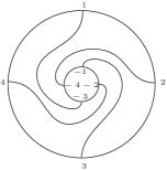
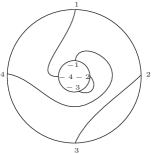
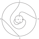
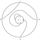
Figure 2. The 5 non-crossing annular pairings corresponding the infinitesimal moment $m^{\prime}_{4}=5$. Note that if $(r,s)$ is a pair then so is $(-r,-s)$.

By Corollary 14 we must find all pairs $(\pi,\epsilon)$ with $\pi\in\mathcal{P}_{2}(n)$ and $\epsilon\in\mathbb{Z}_{2}^{n}$ such that there is at least one pair $(r,s)\in\pi$ such that $\epsilon_{r}=\epsilon_{s}$ and $\#(\gamma\delta\gamma^{-1}\delta\rho)=n$ where $\rho=\epsilon\pi\delta\pi\epsilon$. These are exactly the non-crossing annular pairings of [16, Thm. 6.1] where we have reversed the orientation of the inner circle (see Figure 2). Moreover we do not get all non-crossing annular pairings, only those for which

1. $\rho$ commutes with $\delta$,

2. For all $r\in[n]$, $(r,-r)$ is never a pair of $\rho$.

3. the blocks of $\rho$ come in pairs: if $(r,s)\in\pi$ then $(-r,-s)\in\rho$.

If $r$ and $s$ have opposite signs then $(r,s)$ is a through string, i.e. it connects the two circles. Thus these pairings always connect the two circles.

Notation 16.

We denote by $NC_{2}^{\delta}(n,-n)$ the set of all non-crossing annular pairings $\rho$ that satisfy (i), (ii), (iii) above. By convention $NC_{2}^{\delta}(n,-n)$ is empty for $n$ odd.

We have put a ‘$-$’ sign in front of the second ‘$n$’ to remind us the orientation of the inside circle has been reversed from that used in [16]. Summarizing the discussion above we have the following theorem.

Theorem 17.

Let $X_{N}$ be the $N\times N$ goe and $m_{n}$ the $n^{th}$ moment of the semi-circle law. Then the infinitesimal moments of the goe are given by $m^{\prime}_{n}=\lim_{N}N(\textrm{E}(\textrm{tr}(X_{N}^{n}))-m_{n})=|NC_{2}^{\delta}(n,-n)|$ for $n$ even and $m^{\prime}=0$ for $n$ odd.

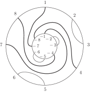
Figure 3. We illustrate here an element of $NC_{2}^{\delta}(8,-8)$. Let $\pi=(1,7)\allowbreak(2,3)\allowbreak(4,8)(5,6)$, and $\epsilon=(1,1,$$-1,1,\allowbreak 1,-1,\allowbreak 1,1)$. Then $\rho=\epsilon\pi\delta\pi\epsilon=(1,-7)\allowbreak(-1,7)(2,3)(-2,-3)(4,-8)(-4,8)\allowbreak(5,6)\allowbreak(-5,-6)$. Note that the symmetry condition $\delta\rho=\rho\delta$ means that once the non-through strings are placed (in this example $(2,4)(5,6)(-2,-4)(-5,-6)$) the through strings are forced; i.e. we must pair $4$ with $-8$ etc. Note that by reversing the order of $\{5,6,7,8\}$ we can make the diagram non-crossing, see Remark 21.

Here are three examples of $(\pi,\epsilon)$’s with all through strings.

or or

Here is an example with 6 through strings and 16 non-through strings.

$\pi=\{(1,2)(3,12)(4,7)(5,6)(8,17)(9,10)(11,18)(13,14)(15,16)\allowbreak(19,22)\allowbreak(20,21)\}$.

Remark 18.

Scrutiny of these examples reveals an important alternative way of describing elements of $NC_{2}^{\delta}(n,-n)$ that will be useful in computing the infinitesimal cumulants $\{\kappa^{\prime}_{n}\}_{n}$ of $(\mu,\mu^{\prime})$. The important property is that if we fuse the thick lines, formed by the through strings, we always get a non-crossing partition. Moreover the thick lines always occur in the same way: if the block formed by the thick lines is $(i_{1},\dots,i_{k})$ then $k=2l$ must be even and the pairs are $(i_{1},i_{l+1})$, $(i_{2},i_{l+2})$, …, $(i_{l},i_{2l})$. Thus given a non-crossing partition $\pi\in NC(n)$ and a block $V\in\pi$ such that $|V|$ is even and all other blocks of $\pi$ have 2 elements we can construct an element of $NC_{2}^{\delta}(n,-n)$.

Definition 19 (c.f.[1, Def. 1] and [14, §6]).

Let $\pi$ be a non-crossing partition in which no block has more than two elements. From $\pi$ create a new partition $\tilde{\pi}$ by joining into a single block all the blocks of $\pi$ of size 1, call this block $V$. If $\tilde{\pi}$ is non-crossing and $|V|$ is even we say that $(\tilde{\pi},V)$ is a non-crossing half-pairing. The blocks of $\pi$ of size 1 are called the through strings. (See Figure 4.) We let $NCC_{2}(n)=\{(\pi,V)\mid\pi\in NC(n),V\in\pi$, $|V|$ is even, and all other blocks of $\pi$ have 2 elements$\}$. By convention $NCC_{2}(n)$ is empty for $n$ odd.

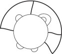
Figure 4. On the left is $\pi$ and on the right is $\tilde{\pi}$.

Remark 20.

From Remark 18 we see that there is a bijection from $NCC_{2}(n)$ to $NC_{2}^{\delta}(n,-n)$ where a pair $(\pi,V)$ with $V$ a block of size $k$ produces a $\rho\in NC_{2}^{\delta}(n,-n)$ with $k$ through strings. By [1, Lemma 13] the number of non-crossing half-pairings with $k$ through strings is $\binom{n}{(n-k)/2}$

Remark 21.

In Figure 3 we presented an example where we have $(\pi,\epsilon)$, a pairing of $[8]$ with crossings and an assignment of signs, we unfolded the diagram into $\rho$, a non-crossing annular pairing and also a non-crossing pairing on a disc. This is in fact a general situation. We rotate the numbers $\{1,2,3,\dots,n\}$ until half the thick lines are in $\{1,2,3,\dots,n/2\}$. Then reverse the numbers $\{n/2+1,\dots,n\}$.

Lemma 22.

Let $n=2m$. The number of non-crossing annular pairings satisfying (i), (ii), and (iii) above is

$$m^{\prime}_{n}=\sum_{k=1}^{m}\binom{n}{m-k}=\frac{1}{2}\Big{(}2^{n}-\binom{n}{m}\Big{)}.$$

Proof.

We know that the number of non-crossing annular pairings of an $(p,q)$-annulus with $l$ through strings is $l\binom{p}{\frac{p-l}{2}}\binom{q}{\frac{q-l}{2}}$ (see e.g. [20, Eq. (11)]). In our situation $p=q=2m$, $l=2k$ is even and the pairings on the circles are symmetric so we only get $\binom{n}{m-k}$ diagrams, because once the non-through strings are placed there is only one way to place the through strings.

$$2\sum_{k=1}^{m}\binom{n}{m-k}=2\bigg{\{}\binom{n}{0}+\binom{n}{1}+\cdots+\binom{n}{m-1}\bigg{\}}$$

$$= \binom{n}{0}+\cdots+\binom{n}{m-1}+\binom{n}{m+1}+\cdots+\binom{n}{n-1}+\binom{n}{n}$$

$$= 2^{n}-\binom{n}{m}.$$

     

Theorem 23.

Let $\nu_{1}=\frac{1}{2}(\delta_{-2}+\delta_{2})$ be the Bernoulli distribution and $d\nu_{2}(t)=\frac{1}{\pi}\frac{1}{\sqrt{4-t^{2}}}\,dt$ be the arcsine law. Let $\mu^{\prime}=\frac{1}{2}(\nu_{1}-\nu_{2})$. Let $X_{N}$ be the $N\times N$ goe and $m_{n}$ the $n^{th}$ moment of the semi-circle law. Then

$$\lim_{N}N(\textrm{E}(\textrm{tr}(X^{n}))-m_{n})=m_{n}^{\prime}$$

and

$$m_{n}^{\prime}=\int t^{n}\,d\mu^{\prime}(t).$$

5. Infinitesimal cumulants of the goe

Recall that if a partition has all blocks of even size then it is called an even partition. We already know that for the infinitesimal goe we have $\kappa_{2}=1$ and all other $\kappa_{n}=0$ (i.e. the semi-circle law). We shall show that $\kappa^{\prime}_{2m}=1$ and $\kappa^{\prime}_{2m-1}=0$ for all $m\geq 1$. This means that for an even non-crossing partition of $[n]$ (using the notation of Eq. (5))

(11) $$\partial\kappa_{\pi}=\begin{cases}\frac{n}{2}&\pi\mbox{\ is a pairing}\\ 1&\pi\ \vtop{\noindent\raggedright has one block of size $k$ and all others of size 2\@add@raggedright}\\ 0&\pi\ \vtop{\noindent\raggedright has at least 2 blocks with more than 2 elements\@add@raggedright}\end{cases}$$

From Kreweras [12, Théorème 4] we know that that number of partitions with one block of size $k>2$ and all others of size 2 is $\binom{n}{\frac{n+k}{2}}$.

Using the cumulant-moment formula (Eq. (6)) we have

$$\kappa^{\prime}_{1}=m^{\prime}_{1}$$

$$\kappa^{\prime}_{2}=m^{\prime}_{2}-2m^{\prime}_{1}m_{1}$$

$$\kappa^{\prime}_{3}=m^{\prime}_{3}-3m^{\prime}_{1}m_{2}-3m_{1}m^{\prime}_{2}+6m^{\prime}_{1}m_{1}m_{1}$$

$$\kappa^{\prime}_{4}=m^{\prime}_{4}-4m^{\prime}_{1}m_{3}-4m_{1}m^{\prime}_{3}-4m^{\prime}_{2}m_{2}+12m^{\prime}_{2}(m_{1})^{2}\\ +24m^{\prime}_{1}m_{2}m_{1}-24m^{\prime}_{1}(m_{1})^{3}$$

All these formulas can be obtained by assuming an implicit dependence on a parameter $t$ and applying $\displaystyle\frac{d}{dt}\Big{|}_{t=0}$ to both sides of

$$\kappa_{n}=\sum_{\pi\in NC(n)}\kappa_{\pi}\mbox{\ with\ }\kappa^{\prime}_{n}=\displaystyle\frac{d}{dt}\Big{|}_{t=0}\kappa_{n}\mbox{\ and\ }m^{\prime}_{n}=\displaystyle\frac{d}{dt}\Big{|}_{t=0}m_{n}.$$

Since $m^{\prime}_{1}=m^{\prime}_{3}=0$ and $m^{\prime}_{2}=1$ and $m^{\prime}_{4}=5$ we have $\kappa^{\prime}_{1}=\kappa^{\prime}_{3}=0$ and $\kappa^{\prime}_{2}=\kappa^{\prime}_{4}=1$.

Lemma 24.

If $n$ is odd then $\kappa^{\prime}_{n}=0$.

Proof.

Let us recall some standard notation. For $\pi\in\mathcal{P}(n)$ we let $m_{\pi}=\prod_{V\in\pi}m_{|V|}$. We set

$$\partial m_{\pi}=\sum_{V\in\pi}m^{\prime}_{|V|}\mathop{\prod_{W\in\pi}}_{W\not=V}m_{|W|}$$

The moment-cumulant formula

$$\kappa_{n}=\sum_{\pi\in NC(n)}\mu(\pi,1_{n})m_{\pi}$$

becomes

$$\kappa^{\prime}_{n}=\sum_{\pi\in NC(n)}\mu(\pi,1_{n})\partial m_{\pi}.$$

We have seen that both $m_{n}=0$ and $m^{\prime}_{n}=0$ for $n$ odd. If $n$ is odd and $\pi\in\mathcal{P}(n)$ then $\pi$ must have a block of odd size. Thus $\partial m_{\pi}=0$. Hence for $n$ odd $\kappa^{\prime}_{n}=0$.             

Theorem 25.

For $n$ even $\kappa^{\prime}_{n}=1$.

Proof.

We have already shown that $\kappa^{\prime}_{2}=\kappa^{\prime}_{4}=1$. Suppose that we have shown that $\kappa^{\prime}_{2}=\cdots=\kappa^{\prime}_{n-2}=1$. We shall prove that $\kappa^{\prime}_{n}=1$. From the infinitesimal moment-cumulant formula (4) we have that

$$m^{\prime}_{n}=\sum_{\pi\in NC(n)}\sum_{V\in\pi}\kappa^{\prime}_{\pi,V}.$$

By induction we have that $\kappa^{\prime}_{\pi,V}=1$ for $(\pi,V)\in NCC_{2}(n)$ and $\pi\not=1_{n}$. Moreover by Lemma 24 we have that $\kappa^{\prime}_{\pi,V}=0$ if $(\pi,V)\not\in NCC_{2}(n)$. Hence

$$m^{\prime}_{n}-\kappa^{\prime}_{n}=\mathop{\sum_{\pi\in NC(n)}}_{\pi\not=1_{n}}\sum_{V\in\pi}\kappa^{\prime}_{\pi,V}=|NCC_{2}(n)|-1.$$

Since we have by Lemma 22 that $m^{\prime}_{n}=|NCC_{2}(n)|$ we must have $\kappa^{\prime}_{n}=1$ as claimed.             

Corollary 26.

For the infinitesimal goe we have the infinitesimal $r$-transform is given by $r(z)=\frac{z}{1-z^{2}}$.

Remark 27.

By Corollary 26 and Eq. (8) we have that the infinitesimal Cauchy transform of $\mu^{\prime}$ is

$$g(z)=-r(G(z))G^{\prime}(z)=\frac{G(z)}{z^{2}-4}=\frac{z-\sqrt{z^{2}-4}}{2(z^{2}-4)}.$$

Note that in accordance with Eq. (1), $g$ has poles at $z=2$ and $z=-2$ each with residue $\frac{1}{4}$.

Now that we have the infinitesimal cumulants we can easily see that independent goe’s cannot be asymptotically free.

Proposition 28.

Let $\{X_{N}\}_{N}$ and $\{Y_{N}\}_{N}$ be independent ensembles of goe random matrices. Then $\{X_{N}\}_{N}$ and $\{Y_{N}\}_{N}$ are not asymptotically infinitesimally free.

Proof.

Suppose $\{X_{N}\}_{N}$ and $\{Y_{N}\}_{N}$ were asymptotically infinitesimally free. Then there would be an infinitesimal probability space $(\mathcal{A},\varphi,\varphi^{\prime})$ and $x,y\in\mathcal{A}$ which are infinitesimally free such that for all $k$

$$\lim_{N}\textrm{E}(\textrm{tr}(X_{N}^{k}))=\varphi(x^{k})\mathrm{\ and\ }\lim_{N}N(\textrm{E}(\textrm{tr}(X_{N}^{k}))-\varphi(x^{k}))=\varphi^{\prime}(x^{k})$$

and

$$\lim_{N}\textrm{E}(\textrm{tr}(Y_{N}^{k}))=\varphi(y^{k})\mathrm{\ and\ }\lim_{N}N(\textrm{E}(\textrm{tr}(Y_{N}^{k}))-\varphi(y^{k}))=\varphi^{\prime}(y^{k}).$$

Let $Z_{N}=\frac{1}{\sqrt{2}}(X_{N}+Y_{N})$ and $z=\frac{1}{\sqrt{2}}(x+y)$. Then by Remark 9, $\{Z_{N}\}_{N}$ is also a goe random matrix and so by Theorem 25, for all $n$

$${\kappa^{\prime}}_{2n}^{(x)}={\kappa^{\prime}}_{2n}^{(y)}={\kappa^{\prime}}_{2n}^{(z)}=1.$$

On the other hand by our assumption of infinitesimal freeness we have by the vanishing of mixed cumulants (Thm. 7) that ${\kappa^{\prime}}_{2n}^{(z)}=2^{-n+1}$. This contradiction shows that the ensembles $\{X_{N}\}_{N}$ and $\{Y_{N}\}_{N}$ cannot be asymptotically infinitesimally free.             

Remark 29.

Independent goe random matrices are not asymptotically second order free but are asymptotically real second order free (see Redelmeier [22]). Thus there may be a positive statement one can make in the orthogonal case, see Remark 37.

6. Asymptotic infinitesimal freeness
for complex wishart matrices

To discuss asymptotic infinitesimal freeness we shall make use of the algebra $\mathbb{C}\langle Y_{1},\dots,Y_{s}\rangle$ of polynomials in the non-commuting variables $Y_{1},\dots,Y_{s}$. Given elements $x_{1},\dots,x_{s}$ in an infinitesimal probability space $(\mathcal{A},\varphi,\varphi^{\prime})$ we get two linear functionals on $\mathbb{C}\langle Y_{1},\dots,Y_{s}\rangle$ given by $\mu(Y_{i_{1}}\cdots Y_{i_{n}})=\varphi(x_{i_{1}}\cdots x_{i_{n}})$ and $\mu^{\prime}(Y_{i_{1}}\cdots T_{i_{n}})=\varphi^{\prime}(x_{i_{1}}\cdots x_{i_{n}})$ for all $i_{1},\dots,i_{n}\in[s]$. We call the pair $(\mu,\mu^{\prime})$ the algebraic infinitesimal distribution of $x_{1},\dots,x_{s}$.

For example if $X^{(N)}_{1},\cdots,X^{(N)}_{s}$ are independent $N\times N$ complex Wishart random matrices then using [16, Cor. 9.6], we can use the $1/N$ expansion of $\textrm{E}(\textrm{tr}(X^{(N)}_{i_{1}}\allowbreak\cdots X^{(N)}_{i_{n}}))$ to define a pair $(\mu_{N},\mu^{\prime}_{N})$. We let for $i_{1},\dots,i_{n}\in[s]$

(12) $$\mu_{N}(Y_{i_{1}}\cdots Y_{i_{n}})=\textrm{E}(\textrm{tr}(X_{i_{1}}\cdots X_{i_{n}}))\mbox{\ and\ }\mu(Y_{i_{1}}\cdots Y_{i_{n}})=\mathop{\sum_{\pi\in NC(n)}}_{\pi\leq\ker(i)}c^{\#(\pi)}.$$

Then we set

$$\mu^{\prime}_{N}(I)=0\mathrm{\ and}$$

(13) $$\mu^{\prime}_{N}(Y_{i_{1}}\cdots Y_{i_{n}})=N(\mu_{N}(Y_{i_{1}}\cdots Y_{i_{n}})-\mu(Y_{i_{1}}\cdots Y_{i_{n}}))$$

Finally we set

(14) $$\mu^{\prime}(Y_{i_{1}}\cdots Y_{i_{n}})=\mathop{\sum_{\pi\in NC(n)}}_{\pi\leq\ker(i)}c^{\prime}\,\#(\pi)\,c^{\#(\pi)-1}.$$

Recall here that $S_{n}$ is the symmetric group on $[n]$, $\gamma_{n}=(1,2,3,\dots,\allowbreak n)$, and $\#(\pi)$ is the number of cycles in the cycle decomposition of $\pi$. Also $\ker(i)\in\mathcal{P}(n)$ is the kernel of $i$ as described in Remark 9 page 9.

Theorem 30.

Let $\{X^{(N)}_{1},\dots,X^{(N)}_{s}\}_{N}$ be an independent family of complex $N\times N$ Wishart matrices. Assume that $\lim_{N}M/N=c$ and $\lim_{N}(M-Nc)=c^{\prime}$. Then $\{X^{(N)}_{1},\dots,X^{(N)}_{s}\}$ are asymptotically infinitesimally free and the infinitesimal cumulants of the limit infinitesimal distribution are given by $\kappa^{\prime}_{n}=c^{\prime}$ for all $n\geq 1$. The limit infinitesimal distribution is $(\mu,\mu^{\prime})$ where $\mu$ is the Marchenko-Pastur distribution with parameter $c$ and $\mu^{\prime}$ is given by

(2) $$d\mu^{\prime}(x)=-c^{\prime}\begin{cases}\phantom{\frac{1}{2}}\delta_{0}-\frac{x+1-c}{2\pi x\sqrt{(b-x)(x-a)}}\,dx&c<1\\ \frac{1}{2}\delta_{0}-\frac{1}{2\pi\sqrt{x(4-x)}}\,dx&c=1\\ \phantom{\frac{1}{2}\delta_{0}}-\frac{x+1-c}{2\pi x\sqrt{(b-x)(x-a)}}\,dx&c>1\\ \end{cases}$$

where $a=(1-\sqrt{c})^{2}$ and $b=(1+\sqrt{c})^{2}$.

Proof.

We shall show that

$$\lim_{N}\mu_{N}=\mu\mbox{\ and\ }\lim_{N}\mu^{\prime}_{N}=\mu^{\prime}.$$

We have from [16, Lemma 7.6]

(15) $$\mu_{N}(Y_{i_{1}}\cdots Y_{i_{n}})=\mathop{\sum_{\pi\in S_{n}}}_{\pi\leq\ker(i)}M^{\#(\pi)}N^{\#(\pi^{-1}\gamma)-(n+1)}\\ =\mathop{\sum_{\pi\in S_{n}}}_{\pi\leq\ker(i)}\Big{(}\frac{M}{N}\Big{)}^{\#(\pi)}N^{\#(\pi)+\#(\pi^{-1}\gamma)-(n+1)}$$

For $\pi\in S_{n}$ we have $\#(\pi)+\#(\pi^{-1}\gamma_{n})=n+1-2g$ for some integer $g\geq 0$. Moreover the permutations $\pi$ for which $\#(\pi)+\#(\pi^{-1}\gamma_{n})=n+1$ are exactly the non-crossing partitions. So for $\pi\in S_{n}\setminus NC(n)$ we have $\#(\pi)+\#(\pi^{-1}\gamma)-n\leq-1$. Thus

$$\lim_{N\rightarrow\infty}\mu_{N}(Y_{i_{1}}\cdots Y_{i_{n}})=\mu(Y_{i_{1}}\cdots Y_{i_{n}}).$$

Since we have that $\pi\leq\ker(i)$ we have that mixed cumulants vanish by the definition of $\mu$ in Equation (12). Thus we have that $X_{1},\dots,X_{s}$ are asymptotically free. Of course this is a known fact, see [5]. Moreover we have

(16) $$\mu_{N}^{\prime}(Y_{i_{1}}\cdots Y_{i_{n}})=\mathop{\sum_{\pi\in NC(n)}}_{\pi\leq\ker(i)}N\Big{(}\Big{(}\frac{M}{N}\Big{)}^{\#(\pi)}-c^{\#(\pi)}\Big{)}\\ \mbox{}+\mathop{\sum_{\pi\in S_{n}\setminus NC(n)}}_{\pi\leq\ker(i)}\Big{(}\frac{M}{N}\Big{)}^{\#(\pi)}N^{\#(\pi)+\#(\pi^{-1}\gamma)-n}$$

For any $\pi$ we have

$$\lim_{N\rightarrow\infty}N\Big{(}\Big{(}\frac{M}{N}\Big{)}^{\#(\pi)}-c^{\#(\pi)}\Big{)}=\#(\pi)c^{\#(\pi)-1}c^{\prime}$$

and for $\pi\in S_{n}\setminus NC(n)$

$$\lim_{N\rightarrow\infty}\Big{(}\frac{M}{N}\Big{)}^{\#(\pi)}N^{\#(\pi)+\#(\pi^{-1}\gamma)-n}=0.$$

Hence

$$\lim_{N\rightarrow\infty}\mu^{\prime}_{N}(Y_{i_{1}}\cdots Y_{i_{n}})=\mathop{\sum_{\pi\in NC(n)}}_{\pi\leq\ker(i)}\#(\pi)c^{\#(\pi)-1}c^{\prime}=\mu^{\prime}(Y_{i_{1}}\cdots Y_{i_{n}}).$$

In the expression

$$\mu^{\prime}(Y_{i_{1}}\cdots Y_{i_{n}})=\mathop{\sum_{\pi\in NC(n)}}_{\pi\leq\ker(i)}\#(\pi)c^{\#(\pi)-1}c^{\prime}$$

the condition $\pi\leq\ker(i)$ shows that mixed infinitesimal cumulants also vanish. Thus $X_{1},\dots,X_{s}$ are asymptotically infinitesimally free.

Note that when $\ker(i)=1_{n}$ the right hand side of Eq. (14) is given by the integral $\int t^{n}\,d\mu^{\prime}(t)$ with this $\mu^{\prime}$ the signed measure in Eq. (2). Recall that $\mu^{\prime}(Y_{1}^{n})=\sum_{\pi\in NC(n)}\partial\kappa_{\pi}$, so Eq. (14) shows that when $\ker(i)=1_{n}$ we have $\kappa^{\prime}_{n}=c^{\prime}$ for all $n$.

Only Equation (2) remains to be proved. We compute the infinitesimal Cauchy transform and then use Stieltjes inversion. We have already shown that $\kappa^{\prime}_{n}=c^{\prime}$ for all $n\geq 1$, thus $r(z)=c^{\prime}/(1-z)$. Hence

$$g(z)=-r(G(z))G^{\prime}(z)\\ =-c^{\prime}\frac{G^{\prime}(z)}{1-G(z)}=\frac{-c^{\prime}}{zP(z)}\frac{(1-c)^{2}-(1+c)z-(1-c)P(z)}{P(z)+z-1+c}$$

where $P(z)=\sqrt{(z-a)(z-b)}$, and we choose the branch as in [19, Ex. 3.6]. Note that both $\big{\{}\mathop{\sum}_{\pi\in NC(n)}\big{(}\frac{M}{N}\big{)}^{\#(\pi)}\big{\}}_{n}$ and $\big{\{}\sum_{\pi\in NC(n)}c^{\#(\pi)}\big{\}}_{n}$ are moment sequences of positive measures, thus $g$ is the limit of the difference of Cauchy transforms of positive measures and so we can recover a signed measure by Stieltjes inversion. Now let $Q(x)=\sqrt{(b-x)(x-a)}$ for $x\in[a,b]$ and $Q(x)=0$ for $x\not\in[a,b]$. For a function $f$ on $\mathbb{C}^{+}$ we let $f(x+i0^{+})=\lim_{\epsilon\rightarrow 0^{+}}f(x+i\epsilon)$. Then for $a\leq x\leq b$

$$-\frac{1}{\pi}\mathrm{Im}(g(x+i0^{+}))=c^{\prime}\frac{x+1-c}{2\pi xQ(x)}.$$

As written above, $g$ has a singularity at $0$. For $a\in\mathbb{R}$ and $z\in\mathbb{C}^{+}$ let us write $\lim_{\sphericalangle z\rightarrow a}$ for the non-tangential limit as $z$ approaches $a$ (see e.g [19, p. 60]). We have $\lim_{\sphericalangle z\rightarrow 0}P(z)+z-1+c=0$ when $c>1$, so $\lim_{\sphericalangle z\rightarrow 0}\frac{P(z)+z-1+c}{z}=1+P^{\prime}(0)=1+\frac{1+c}{c-1}=\frac{2c}{c-1}$. From the equation for $g$ above we have

$$zg(z)=\frac{c^{\prime}(1-c)}{P(z)}\Big{\{}1+\frac{2c}{1-c}\frac{z}{P(z)+z-1+c}\Big{\}}$$

and thus $\lim_{\sphericalangle z\rightarrow 0}zg(z)=0$; so the singularity at $0$ is removable. When $c<1$ we have $\lim_{\sphericalangle z\rightarrow 0}P(z)+z-1+c=2(c-1)\not=0$. Thus

$$\lim_{\sphericalangle z\rightarrow 0}\frac{z}{P(z)+z-1+c}=0$$

and hence $\lim_{\sphericalangle z\rightarrow 0}zg(z)=\frac{c^{\prime}(1-c)}{P(0)}=-c^{\prime}$. When $c=1$ we have

$$zg(z)=\frac{2c^{\prime}}{z-4+P(z)}.$$

and thus $\lim_{\sphericalangle z\rightarrow 0}zg(z)=-\frac{c^{\prime}}{2}$. Summarizing we have

$$\lim_{\sphericalangle z\rightarrow 0}zg(z)=\begin{cases}-c^{\prime}.&c<1\\ -\frac{c^{\prime}}{2}&c=1\\ 0&c>1\end{cases}$$

We capture the weight of the mass at $0$ by [19, Prop. 3.8]. The singularities at $a$ and $b$ are removable.             

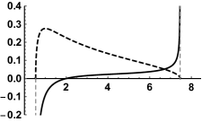
Figure 5. The densities for $\mu$ (dashed) and $\mu^{\prime}$ (solid) when $c=3$ and $c^{\prime}=1$.

Remark 31.

To make the two distributions explicit let us summarize. For $c>0$, $a=(1-\sqrt{c})^{2}$ and $b=(1+\sqrt{c})^{2}$ we have

(17) $$\int_{a}^{b}x^{n}\frac{\sqrt{(b-x)(x-a)}}{2\pi x}\,dx=\sum_{\pi\in NC(n)}c^{\#(\pi)}$$

(18) $$\int_{a}^{b}x^{n}\frac{c^{\prime}(x+1-c)}{2\pi x\sqrt{(b-x)(x-a)}}\,dx=\sum_{\pi\in NC(n)}\#(\pi)c^{\#(\pi)-1}c^{\prime}.$$

Note that we can also obtain (18) from (17) by formal differentiation by $t$. Namely suppose that $c$ is an implicit function of $t$ and $c^{\prime}=\frac{d}{dt}\big{|}_{t=0}c$. Then $(b-x)(x-a)=-x^{2}+2(1+c)x-(1-c)^{2}$. So

$$\frac{d}{dt}\Big{|}_{t=0}(b-x)(x-a)=2c^{\prime}(x+1-c)$$

and thus

$$\frac{d}{dt}\Big{|}_{t=0}\frac{\sqrt{(b-x)(x-a)}}{2\pi x}=\frac{c^{\prime}(x+1-c)}{2\pi x\sqrt{(b-x)(x-a)}}.$$

For $c\not=1$, this formal operation picks up the mass at $0$ if we say that $\frac{d}{dt}\big{|}_{t=0}(1-c)\delta_{0}=-c^{\prime}\delta_{0}$. At $c=1$ it seems a more delicate formal argument is required.

7. A universal rule for the goe and constant matrices

We have already shown that independent goe ensembles are not asymptotically free. In this section we shall go a little further and give a rule that shows a different kind of freeness applies in the orthogonal case. First let us recall a formula from [10, Eq.(5.1)] for when $a_{1},\dots,a_{n}\in\mathcal{A}_{1}$, $b_{1},\dots,b_{n}\in\mathcal{A}_{2}$ and $\mathcal{A}_{1}$ and $\mathcal{A}_{2}$ are infinitesimally free

(19) $$\varphi^{\prime}(a_{1}b_{1}a_{2}b_{2}\cdots a_{n}b_{n})\\ =\sum_{\pi\in NC(n)}\{\kappa_{\pi}(a_{1},\cdots,a_{n})\ \partial\varphi_{K(\pi)}(b_{1},\cdots,b_{n})\\ \mbox{}+\partial\kappa_{\pi}(a_{1},\cdots,a_{n})\ \varphi_{K(\pi)}(b_{1},\cdots,b_{n})\}$$

where $K(\pi)$ is the Kreweras complement of $\pi$.

Suppose we have for each $N$, $A^{(N)}_{1},\dots,A^{(N)}_{s}$, $N\times N$ matrices that have a joint limit $t$-distribution. Recall from [17] this means that $\{A^{(N)}_{1},A^{(N)t}_{1},\dots,A^{(N)}_{s},A^{(N)t}_{s}\}$ has a joint limit distribution. Using our convention that $A_{i}^{(1)}=A_{i}$ and $A_{i}^{(-1)}=A_{i}^{t}$ this means that for every $i_{1},\dots,i_{n}$ and every $\epsilon_{1},\dots,\epsilon_{s}\in\{-1,1\}$ the limit

$$\lim_{N}\textrm{tr}(A^{(N)(\epsilon_{1})}_{i_{1}}\cdots A^{(N)(\epsilon_{n})}_{i_{n}})$$

exists; we denote this limit by $\varphi(a_{1}^{(\epsilon_{1})}\cdots a_{n}^{(\epsilon_{n})})$ where $a_{1}\dots,a_{s},a_{1}^{t},\dots,\allowbreak a^{t}_{s}$ are in some non-commutative infinitesimal space $(\mathcal{A},\varphi,\varphi^{\prime})$ with a transpose $a\mapsto a^{t}$. Let us further suppose that $A_{1},\dots,A_{s}$ have a joint infinitesimal distribution. This means that for all $i_{1},\dots,i_{n}$ we have that

(20) $$\varphi^{\prime}(a_{i_{1}}\cdots a_{i_{n}})=\lim_{N}N(\textrm{tr}(A_{i_{1}}\cdots A_{i_{n}})-\varphi(a_{i_{1}}\cdots a_{i_{n}}))$$

exists. In order to describe the limiting behaviours we need some notation.

Figure 6. The non-crossing annular permutation $\pi=(1,2,8)(3)(4,6,7)(5)$.

Notation 32.

Recall from [16, Def. 3.5] that for integers $m,n\geq 1$ we let $S_{NC}(m,n)$ be the non-crossing annular permutations. We shall briefly recall the details. Let $\gamma_{m,n}=(1,2,3,\dots,m)(m+1,\dots,m+n)$ be the permutation in $S_{m+n}$ with two cycles. A permutation $\pi\in S_{m+n}$ is non-crossing annular if $\pi$ $\#(\pi)+\#(\pi^{-1}\gamma_{m,n})=m+n$ and $\pi$ has at least one cycle that connects $\{1,2,\dots,m\}$ to $\{m+1,\dots,m+n\}$. Such cycles are called through cycles. See Figure 6.

Remark 33.

Now let us recall a basic formula. Let $\sigma\in S_{n}$ be a permutation and $A_{1},\dots A_{n}$ be $N\times N$ matrices. We recall that $\textrm{Tr}_{\sigma}(A_{1},\dots,A_{n})$ is the product over the cycles of $\sigma$ of traces of products of $A$’s. More precisely

$$\textrm{Tr}_{\sigma}(A_{1},\dots,A_{n})=\mathop{\prod_{c\in\sigma}}_{c=(i_{1},\dots,i_{k})}\textrm{Tr}(A_{i_{1}}\cdots A_{i_{k}}).$$

It is a standard result that

$$\textrm{Tr}_{\sigma}(A_{1},\dots,A_{n})=\sum_{i_{1},\dots i_{n}=1}^{N}a^{(1)}_{i_{1}i_{\sigma(1)}}a^{(2)}_{i_{2}i_{\sigma(2)}}\cdots a^{(n)}_{i_{n}i_{\sigma(n)}}.$$

We then let

$$\textrm{tr}_{\sigma}(A_{1},\dots,A_{n})=N^{-\#(\sigma)}\textrm{Tr}_{\sigma}(A_{1},\dots,A_{n}).$$

Let us recall next a formula from [17, Lemma 5]. If $p\in\mathcal{P}_{2}(\pm n)$ is a pairing of $[\pm n]$ then there are $\sigma\in S_{n}$ and $\eta\in\mathbb{Z}_{2}^{n}$ such that

$$\mathop{\sum_{i_{\pm 1},\dots,i_{\pm n}=1}}_{\ker(i)\geq p}^{N}a^{(1)}_{i_{1}i_{-1}}\cdots a^{(n)}_{i_{n}i_{-n}}=\textrm{Tr}_{\sigma}\big{(}A^{(\eta_{1})},\dots,A^{(\eta_{n})}\big{)}$$

which are obtained as follows. According to Remark 11 the cycles of $p\delta$ occur in pairs so we may write

$$p\delta=c_{1}c^{\prime}_{1}\cdots c_{k}c^{\prime}_{k}$$

where $c^{\prime}_{i}=\delta c_{i}^{-1}\delta$. If $c_{i}=(j_{1},\dots,j_{r})$ with $j_{1},\dots,j_{r}\in[\pm n]$ we let $\tilde{c}_{i}=(|j_{1}|,\dots,|j_{r}|)$ and $\eta_{j_{i}}=j_{i}/|j_{i}|$. For example if $n=4$ and $p=(1,3)(-1,2)(-2,-3)(4,-4)$ then $p\delta=(1,2,-3)(4)(-1,3,-2)(-4)$. So $\sigma=(1,2,3)(4)$ and $\eta=(1,1,-1,1)$. Thus

$$\mathop{\sum_{i_{\pm 1},i_{\pm 2},i_{\pm 3},i_{\pm 4}=1}}_{\ker(i)\geq p}^{N}a^{(1)}_{i_{1}i_{-1}}a^{(2)}_{i_{2}i_{-2}}a^{(3)}_{i_{3}i_{-3}}a^{(4)}_{i_{4}i_{-4}}=\textrm{Tr}(A_{1}A_{2}A^{t}_{3})\textrm{Tr}(A_{4}).$$

Note that there is not a canonical choice of a representative $\sigma$ because we have to choose one cycle from each pair $c_{i}$ or $c^{\prime}_{i}$. However because $\textrm{Tr}(A_{1}\cdots A_{k})=\textrm{Tr}(A_{k}^{t}\cdots A_{1}^{t})$, the value of $\textrm{Tr}_{\sigma}\big{(}A_{1}^{(\eta_{1})},\dots,A_{n}^{(\eta_{n})}\big{)}$ is independent of the choices.

Lemma 34.

Suppose that $X$ is the $N\times N$ goe and $A_{1},\dots,A_{n}$ is a set of constant matrices. Then

(21) $$\textrm{E}(\textrm{tr}(XA_{1}\cdots XA_{n}))=\frac{N^{\#(\sigma)-(n/2+1)}}{2^{n/2}}\mathop{\sum_{\pi\in\mathcal{P}_{2}(n)}}_{\epsilon\in\mathbb{Z}_{2}^{n}}\textrm{tr}_{\sigma}(A_{1}^{(\eta_{1})},\dots,A_{n}^{(\eta_{n})})$$

where $(\sigma,\eta)$ depends on the pair $(\pi,\epsilon)$ in the manner described in Remark 33.

Proof.

We write $X=\frac{1}{\sqrt{2N}}(G+G^{t})$. We repeat the calculation from Lemma 10, now with the $A$’s inserted.

$$\textrm{E}(\textrm{Tr}(XA_{1}\cdots XA_{n}))$$

$$= (2N)^{-n/2}\sum_{\epsilon\in\mathbb{Z}_{2}^{n}}\textrm{E}(\textrm{Tr}(G^{(\epsilon_{1})}A_{1}\cdots G^{(\epsilon_{n})}A_{n}))$$

$$= (2N)^{-n/2}\sum_{\epsilon\in\mathbb{Z}_{2}^{n}}\sum_{i_{\pm 1},\dots,i_{\pm n}}\textrm{E}((G^{(\epsilon_{1})})_{i_{1}i_{-1}}\cdots(G^{(\epsilon_{1})})_{i_{n}i_{-n}})$$

$$\qquad\mbox{}\times a^{(1)}_{i_{-1}i_{2}}\cdots a^{(n)}_{i_{-n}i_{1}}$$

$$= (2N)^{-n/2}\sum_{\epsilon\in\mathbb{Z}_{2}^{n}}\sum_{j_{\pm 1},\dots,j_{\pm n}}\textrm{E}(g_{j_{1}j_{-1}}\cdots g_{j_{n}j_{-n}})$$

$$\qquad\mbox{}\times a^{(1)}_{j_{-\epsilon(1)}j_{\epsilon(2)}}\cdots a^{(n)}_{j_{-\epsilon(n)}j_{\epsilon(1)}}\qquad\mbox{(letting\ }j=i\circ\epsilon)$$

$$= (2N)^{-n/2}\sum_{\epsilon\in\mathbb{Z}_{2}^{n}}\sum_{j_{\pm 1},\dots,j_{\pm n}}\sum_{\pi\in\mathcal{P}_{2}(n)}\mathds{1}_{\ker(j)\geq\pi\delta\pi\delta}$$

$$\qquad\mbox{}\times a^{(1)}_{j_{-\epsilon(1)}j_{\epsilon(2)}}\cdots a^{(n)}_{j_{-\epsilon(n)}j_{\epsilon(1)}}$$

$$\kern 140.0pt\mbox{(then letting\ }i=j\circ\delta\gamma^{-1}\epsilon)$$

$$= (2N)^{-n/2}\sum_{\pi,\epsilon}\mathop{\sum_{i_{\pm 1},\dots,i_{\pm n}}}_{\ker(i)\geq\delta\gamma^{-1}\epsilon\pi\delta\pi\delta\epsilon\gamma\delta}a^{(1)}_{i_{1}i_{-1}}\cdots a^{(n)}_{i_{n}i_{-n}}.$$

Note that $\delta\gamma^{-1}\epsilon\pi\delta\pi\delta\epsilon\gamma\delta$ is a pairing so that we can now write the last term using Remark 33. Let $\rho=\epsilon\pi\delta\pi\epsilon$. Then $\delta\gamma^{-1}\epsilon\pi\delta\pi\delta\epsilon\gamma\delta=\delta\gamma^{-1}\delta\rho\gamma\delta$. Hence $\delta\gamma^{-1}\epsilon\pi\delta\pi\delta\epsilon\gamma\delta\cdot\delta=\delta\gamma^{-1}\delta\cdot\rho\cdot\gamma$. So by Remark 33 there is a pair $(\sigma,\eta)\in S_{n}\times\mathbb{Z}_{2}^{n}$ such that

$$\mathop{\sum_{i_{\pm 1},\dots,i_{\pm n}}}_{\ker(i)\geq\delta\gamma^{-1}\epsilon\pi\delta\pi\delta\epsilon\gamma\delta}a^{(1)}_{i_{1}i_{-1}}\cdots a^{(n)}_{i_{n}i_{-n}}=\textrm{Tr}_{\sigma}(A_{1}^{(\eta_{1})},\dots,A_{n}^{(\eta_{n})}).$$

Hence

$$\textrm{E}(\textrm{tr}(XA_{1}\cdots XA_{n}))=\frac{N^{\#(\sigma)-(n/2+1)}}{2^{n/2}}\mathop{\sum_{\pi\in\mathcal{P}_{2}(n)}}_{\epsilon\in\mathbb{Z}_{2}^{n}}\textrm{tr}_{\sigma}(A_{1}^{(\eta_{1})},\dots,A_{n}^{(\eta_{n})})$$

where $(\sigma,\eta)$ depends on the pair $(\pi,\epsilon)$ in the manner described in Remark 33.             

In Remark 13 we showed that $\#(\epsilon\gamma\delta\gamma^{-1}\epsilon\vee\pi\delta\pi\delta)\leq n/2+1$ with equality only if $\pi\in NC_{2}(n)$ and $\epsilon_{r}=-\epsilon_{s}$ for all $(r,s)\in\pi$. Moreover in this case $\rho=\epsilon\pi\delta\pi\epsilon=\pi\delta\pi\delta$ so that $\delta\gamma^{-1}\delta\rho\gamma=\pi\gamma\delta\gamma^{-1}\pi\delta$ and hence $\sigma=\pi\gamma=K(\pi)$ and $\eta\equiv 1$. Also for a given $\pi$ there are $2^{n/2}$ choices of $\epsilon$ such that $\epsilon_{r}=-\epsilon_{s}$ for all $(r,s)\in\pi$. Hence the highest order, $O(1)$, term of $\textrm{E}(\textrm{tr}(XA_{1}\cdots XA_{n}))$ is

$$\sum_{\pi\in NC_{2}(n)}\textrm{tr}_{K(\pi)}(A_{1},\dots,A_{n}).$$

Under our assumption of the existence of an infinitesimal limit (Eq. (20)) we have

$$\lim_{N}N\Big{(}\sum_{\pi\in NC_{2}(n)}\textrm{tr}_{K(\pi)}(A_{1},\dots,A_{n})-\sum_{\pi\in NC_{2}(n)}\varphi_{K(\pi)}(a_{1},\dots,a_{n})\Big{)}\\ =\sum_{\pi\in NC_{2}(n)}\partial\varphi_{K(\pi)}(a_{1},\dots,a_{n})\\ =\sum_{\pi\in NC(n)}\kappa_{\pi}(x,\dots,x)\ \partial\varphi_{K(\pi)}(a_{1},\dots,a_{n}),$$

where the last equality holds because $x$ is a semi-circular operator.

In Corollary 14 we showed that the second highest order, $O(N^{-1})$, term in Eq. (21) is when $\#(\epsilon\gamma\delta\gamma^{-1}\epsilon\vee\pi\delta\pi\delta)=n/2$ and this only occurs when $\rho\in NC_{2}^{\delta}(n,-n)$. So this term is

(22) $$2^{-n/2}\mathop{\sum_{\pi\in\mathcal{P}_{2}(n)}}_{\epsilon\in\mathbb{Z}_{2}^{n}}\textrm{tr}_{\sigma}(A_{1}^{(\eta_{1})},\dots,A_{n}^{(\eta_{n})})$$

where $(\pi,\epsilon)$ are such that $\#(\epsilon\gamma\delta\gamma^{-1}\epsilon\vee\pi\delta\pi\delta)=n/2$ and $(\sigma,\eta)$ depends on the pair $(\pi,\epsilon)$ in the manner described in Remark 33. The element $\rho=\epsilon\pi\delta\pi\epsilon$ produced from such a pair is in $NC_{2}^{\delta}(n-n)$ and is independent of $\epsilon$ in the sense that for each pair $(r,s)\in\pi$, $\rho$ only depends on the product $\epsilon_{r}\epsilon_{s}$. There are $2^{n/2}$ ways of choosing an $\epsilon$ for a fixed assignment of signs $\epsilon_{r}\epsilon_{s}$ for each $(r,s)\in\pi$. Moreover every $\rho\in NC_{2}^{\delta}(n,-n)$ can be obtained from some pair $(\pi,\epsilon)$. To see this start with a $\rho\in NC_{2}^{\delta}(n,-n)$ and for each pair $(r,s)\in\rho$ let $(|r|,|s|)$ be a pair of $\pi$. Because of the symmetry $\delta\rho\delta=\rho$ each $(|r|,|s|)$ will appear twice. Choose $\epsilon$ so that for each $(r,s)\in\rho$ we have $\epsilon_{r}\epsilon_{s}=-1$ if $(r,s)$ is not a through string of $\rho$ and $\epsilon_{r}\epsilon_{s}=1$ if $(r,s)$ is a through string of $\rho$. Thus we may write Eq. (22) as

$$\sum_{\rho\in NC_{2}^{\delta}(n,-n)}\textrm{tr}_{\sigma}(A_{1}^{(\eta_{1})},\dots,A_{n}^{(\eta_{n})}).$$

and as $N\rightarrow\infty$ we get

$$\sum_{\rho\in NC_{2}^{\delta}(n,-n)}\varphi_{\sigma}(a_{1}^{(\eta_{1})},\dots,a_{n}^{(\eta_{n})}).$$

Putting these two terms together we get

$$\varphi^{\prime}(xa_{1}\cdots xa_{n})\\ =\lim_{N}N\big{(}\textrm{E}(\textrm{tr}(XA_{1}\cdots XA_{n}))-\sum_{\pi\in NC_{2}(n)}\varphi_{K(\pi)}(a_{1},\dots,a_{n})\big{)}\\ =\sum_{\pi\in NC_{2}(n)}\partial\varphi_{K(\pi)}(a_{1},\dots,a_{n})+\sum_{\rho\in NC_{2}^{\delta}(n,-n)}\varphi_{\sigma}(a_{1}^{(\eta_{1})},\dots,a_{n}^{(\eta_{n})}).$$

Notation 35.

Given $\rho\in NC_{2}^{\delta}(n,-n)$ we construct $(\sigma,\eta)$ as in Remark 33 and we denote $\varphi_{\sigma}(a_{1}^{(\eta_{1})},\dots,a_{n}^{(\eta_{n})})$ by $\varphi_{K^{\delta}(\rho)}(a_{1},\dots,a_{n})$. The justification for this notation is that the pair $(\sigma,\eta)$ comes from the cycles of $\delta\gamma^{-1}\delta\rho\gamma$ which can be thought of as a type $B$ Kreweras complement. See Figure 7.

Figure 7. If we let $\pi=(1,7)(2,3)(4,8)(5,6)\in\mathcal{P}_{2}(8)$ and $\epsilon=(1,1,\allowbreak-1,1,1,-1,1,1)$, then $\rho=\epsilon\pi\delta\pi\epsilon=(1,-7)(2,3)\allowbreak(4,-8)\allowbreak(5,6)(-1,7)\allowbreak(-2,-3)(-4,8)(-5,-6)$. We compute $\delta\gamma^{-1}\delta\rho\gamma=(1,3,-7)(2)\allowbreak(4,6,-8)\allowbreak(5)\allowbreak(-1,7,-3)\allowbreak(-2)\allowbreak(-4,8,-6)\allowbreak(-5)$. Then $\sigma=(1,3,7)(2)(4,6,8)(5)$ and $\eta=(1,1,1,1,1,1,-1,-1)$. We have $\varphi_{K^{\delta}(\rho)}(a_{1},a_{2},a_{3},a_{4},a_{5},a_{6},a_{7},a_{8})$ $=\varphi(a_{1}a_{3}a_{7}^{t})\varphi(a_{2})\varphi(a_{4}a_{6}a_{8}^{t})\varphi(a_{5})$.

Theorem 36.

Suppose that $X$ is the $N\times N$ goe and $A_{1},\dots,A_{n}$ is a set of constant matrices such that the $A$’s have a joint infinitesimal limit distribution and $A_{1},\dots,A_{n},A_{1}^{t},\dots,A_{n}^{t}$ also have a joint limit distribution. Then

$$\lim_{N}N(\textrm{E}(\textrm{tr}(XA_{1}\cdots XA_{n}))-\sum_{\pi\in NC(n)}\kappa_{\pi}(x,\dots,x)\varphi_{K(\pi)}(a_{1},\dots,a_{n}))$$

$$=\sum_{\pi\in NC(n)}\kappa_{\pi}(x,x,\dots,x)\partial\varphi_{K(\pi)}(a_{i_{1}},a_{i_{2}},\dots a_{i_{n}})$$

$$\mbox{}+\sum_{\rho\in NC_{2}^{\delta}(n,-n)}\kappa_{\rho}(x,\dots,x)\varphi_{K^{\delta}(\rho)}(a_{1},\dots,a_{n}).$$

8. concluding remarks

Remark 37.

By writing the second term as a sum over $NC_{2}^{\delta}(n,-n)$ we do not need to have $\partial\kappa_{\rho}$ as in equation (19) on p. 19. However, since there is a bijective map from $NCC_{2}(n)$ to $NC_{2}^{\delta}(n,\allowbreak-n)$ (see the paragraph above and Remark 20) and $\partial\kappa_{\pi}(x,\dots,x)\not=0$ only for elements of $NCC_{2}(n)$ (c.f. Eq. (11) on p. 11), there should be way of writing the second term above as a sum over $NC(n)$. This would make it closer to the equation (19) for infinitesimal freeness.

Remark 38.

As we have seen, the fact that the genus expansion for the complex Wishart means that the infinitesimal cumulants are fairly simple: $\kappa^{\prime}_{n}=c^{\prime}$ for all $n$. In a follow-up paper we shall compute the infinitesimal cumulants of a real Wishart matrix. We get the $c^{\prime}$ term as above plus a polynomial in $c$.

M

References

[1] C. Armstrong, J. A. Mingo, R. Speicher,
J. C. H. Wilson, The Non-Commutative Cycle Lemma,
J. of Comb. Thry., Ser. A 117
(2010). 1158-1166.
[2] Z. D. Bai and J. Silverstein,
Analysis of Large Dimensional Random Matrices,
Springer Series in Statistics, 2009.
[3] S. Belinschi and D. Shlyakhtenko, Free
Probability of Type B: Analytic Interpretation and
Applications, Amer. J. Math.134 (2012),
193-234.
[4] P. Biane, F. Goodman, and A. Nica,
Non-crossing Cumulants of Type B,
Trans. Amer. Math. Soc.355 (2003),
2263-2303.
[5] M. Capitaine, M. Casalis.
Asymptotic freeness by generalized moments for Gaussian and Wishart matrices.
Application to Beta random matrices, Indiana Univ. Math. J.53 2004, 397-431.
[6] B. Collins, J. A. Mingo,
P. Śniady, and R. Speicher,
Second Order
Freeness and Fluctuations of Random Matrices:
III. Higher Order Freeness and Free Cumulants,
Documenta Math., 12 (2007), 1-70.
[7] I. Dumitriu and A. Edelman, Global Spectrum
fluctuations for the -Hermite and -Laguerre
ensembles via matrix models, J. Math. Phy.,
47, 063302 (2006).
[8] N. Enriquez and L. Ménard, Asymptotic
Expansion of the Expected Spectral Measure of Wigner
Matrices, Electron. Commun. Probab.21
(2016), no. 58, 1-11.
[9] M. Février, Higher order infinitesimal
freeness. Indiana Univ. Math. J.61
(2012), 249-295.
[10] M. Février and A. Nica, Infinitesimal
non-crossing cumulants and free probability of type B,
J. Funct. Anal.258 (2010), 2983-3023.
[11] I. Goulden and D. Jackson, Maps in Locally Orientable
Surfaces and Integrals over Real Symmetric Surfaces,
Can. J. Math., 49 (1997), 865-882.
[12] G. Kreweras, Sur les partitions non
croisées d’un cycle, Discrete Math.1
(1972), 333-350.
[13] K. Johansson, On fluctuations of eigenvalues of
random Hermitian matrices, Duke Math. J.91 (1998), 151-204.
[14] T. Kusalik, J. A. Mingo, and R. Speicher,
Orthogonal polynomials and fluctuations of random
matrices, J. Reine Angew. Math., 604 (2007),
1 - 46.
[15] M. Ledoux, A recursion formula for the moments
of the Gaussian orthogonal ensemble, Annales de
l’I. H. P.–Probabilités et Statistiques,
45 (2009), 754-769.
[16] J. A. Mingo and A. Nica, Annular Noncrossing
Permutations and Partitions, and Second Order Asymptotics
for Random Matrices, Int. Math. Res. Not. 2004,
no. 28, 1413-1460.
[17] J. A. Mingo and M. Popa, Real second order
freeness and Haar orthogonal matrices,
J. Math. Phy.54 (2013), 051701, 1-35.
[18] J. A. Mingo and R. Speicher,
Second
Order Freeness and Fluctuations of Random Matrices: I.
Gaussian and Wishart matrices and Cyclic Fock spaces,
J. Funct. Anal., 235, (2006),
226-270.
[19] J. A. Mingo and R. Speicher, Free
Probability and Random Matrices, Fields Institute Communications
35, Springer Nature, 2017.
[20] J. A. Mingo, E. Tan, and R. Speicher, Second
Order Cumulants of Products,
Trans. Amer. Math. Soc.361 (2009),
4571-4781.
[21] A. Nica and R. Speicher, Lectures on
the Combinatorics of Free Probability, Cambridge
Univ. Press, 2006.
[22] C. E. I. Redelmeier, Real second-order
freeness and the asymptotic real second-order freeness of
several real matrix ensembles,
Int. Math. Res. Not.2014, no. 12,
pp. 3353-3395.
[23] D. Shlyakhtenko, Free Probability of Type B and
Asymptotics of Finite Rank Perturbations of Random
Matrices, Indiana Univ. Math. J.67
(2018), 971-991.
[24] D. Voiculescu, Limit laws for random
matrices and free products, Invent. Math.104 (1991), 201–220.
[25] D.-V. Voiculescu, K. Dykema, A. Nica,
Free Random Variables, CRM Monograph Series,
1, 1992.