Machine-learning error models for approximate solutions to
parameterized systems of nonlinear equations

Abstract

This work proposes a machine-learning framework for constructing statistical models of errors incurred by approximate solutions to parameterized systems of nonlinear equations. These approximate solutions may arise from early termination of an iterative method, a lower-fidelity model, or a projection-based reduced-order model, for example. The proposed statistical model comprises the sum of a deterministic regression-function model and a stochastic noise model. The method constructs the regression-function model by applying regression techniques from machine learning (e.g., support vector regression, artificial neural networks) to map features (i.e., error indicators such as sampled elements of the residual) to a prediction of the approximate-solution error. The method constructs the noise model as a mean-zero Gaussian random variable whose variance is computed as the sample variance of the approximate-solution error on a test set; this variance can be interpreted as the epistemic uncertainty introduced by the approximate solution. This work considers a wide range of feature-engineering methods, data-set-construction techniques, and regression techniques that aim to ensure that (1) the features are cheaply computable, (2) the noise model exhibits low variance (i.e., low epistemic uncertainty introduced), and (3) the regression model generalizes to independent test data. Numerical experiments performed on several computational-mechanics problems and types of approximate solutions demonstrate the ability of the method to generate statistical models of the error that satisfy these criteria and significantly outperform more commonly adopted approaches for error modeling.

1 Introduction

Myriad decision-making applications in science and engineering are many-query in nature, as they require a parameterized computational model to be simulated for a large number of parameter instances; examples include design optimization, where each parameter instance corresponds to a different candidate system design; uncertainty propagation, where each parameter instance corresponds to a realization of a random variable; and Bayesian inference, where each parameter instance corresponds to a sample from a posterior distribution. Oftentimes, the computational model in these contexts corresponds to a large-scale system of parameterized nonlinear algebraic equations; this occurs, for example, when the model associates with the spatial discretization of a system of parameterized, nonlinear, stationary partial differential equations.

In such cases, it is prohibitively expensive to compute an exact solution to the system of nonlinear equations for each query. Instead, computationally inexpensive approximate solutions are often employed for tractability; examples include inexact solutions computed from early termination of an iterative method (e.g., Newton’s method); solutions computed from lower-fidelity models (e.g., a coarse mesh, lower finite-element order); and solutions computed from projection-based reduced-order models (ROMs) (e.g., proper orthogonal decomposition with Galerkin projection). However, such approximations introduce an error that should be quantified and accounted for in the resulting analysis. In the context of uncertainty quantification, this error can be interpreted as a source of epistemic uncertainty; as such, it is natural to quantify the error in a statistical manner. Researchers have developed three strategies to quantify the error in such approximate solutions: (1) error indicators, (2) rigorous a posteriori error bounds, and (3) error models.

Error indicators are computable quantities that are informative of the approximate-solution error; they do not rigorously bound the error, nor do they generally produce an unbiased prediction of the error or an estimate of the variance in the prediction. One example is the (dual) norm of the residual evaluated at the approximate solution. This quantity is informative of the error, as it appears as a term in residual-based a posteriori error bounds. As such, it is often used as a termination criterion for iterative linear and nonlinear solvers, as well as for greedy methods that determine snapshot-collection parameter instances during (offline) ROM construction [1, 2, 3, 4, 5, 6] and when deploying ROMs within a trust-region setting [7, 8]. Unfortunately, computing the residual norm is typically computationally costly, as its evaluation incurs an operation count that scales with the dimension of the original problem unless the residual is linear in the solution and affine in functions of the parameters. Another commonly used error indicator is the dual-weighted residual (i.e., adjoint-based error estimator), which provides a first-order approximation of the error in a quantity of interest. This approach is often employed for goal-oriented error estimation (and adaptive refinement) for finite-element [9, 10, 11, 12], finite-volume [13, 14, 15], and discontinuous-Galerkin discretizations [16, 17], as well as for model reduction [18, 19]. Unfortunately, dual-weighted residuals are often difficult to implement, as they require solving a dual linear system whose matrix is the transpose of the residual Jacobian; this is not always possible, for example, when the Jacobian is available only as a black-box operator. Furthermore, computing the dual-weighted residual is computationally costly, as the dimension of the dual linear system is the same as that of the original nonlinear system; this cost can be mitigated if the dual linear solve is approximated using, for example, a lower-fidelity model or reduced-order model. A recently developed approach computes randomized approximations of normed solution errors for parameterized linear systems, wherein the error estimate is indeed unbiased and yields probabilistic error bounds [20].

Rigorous a posteriori error bounds are quantities that bound either the normed solution error or the quantity-of-interest error arising from an approximate solution. These error bounds are typically residual based (i.e., the (dual) norm of the residual appears as a term in the bound) and were pioneered in the reduced-basis community [21, 22]. Although these quantities rigorously bound the error, they are typically not sharp, often overpredicting the error by orders of magnitude. Additionally, they can be challenging to implement, as they require Lipschitz or inf–sup constants to be estimated or bounded, which incurs additional computational cost and can further degrade the bounds’ sharpness [23, 24]. In the reduced-basis context, a recently proposed hierarchical error estimator can yield sharper estimates without the need to compute these constants, at the cost of solving a higher-dimensional reduced-order model [25]. Finally, these (deterministic) bounds are of limited utility in an uncertainty-quantification setting, where a statistical model of the error is more readily integrable into the uncertainty analysis.

Error models directly model the error incurred by an approximate solution. In contrast to error indicators and rigorous error bounds, error models often yield a more accurate approximation of the error; furthermore, they facilitate integration of approximate solutions into uncertainty quantification when the error model is statistical in nature. The most common error-modeling approach is to directly model the mapping from model parameters to the error in a quantity of interest. This is an a priori error model, as it does not leverage any data generated by the approximate solution (e.g., the residual norm) at new parameter instances. This approach was developed independently by the optimization community and the model-calibration community. In the optimization community, the technique is often referred to as a ‘multifidelity correction’, wherein the modeled error corresponds to the error between low- and high-fidelity models. Here, the error model is constructed to enforce either ‘global’ zeroth-order consistency between the corrected low-fidelity-model prediction and the high-fidelity-model prediction at training points [26, 27, 28, 29], or ‘local’ first- or second-order consistency at trust-region centers [30, 31]. In the model-calibration community, the technique is referred to as computing a ‘model inadequacy’ or ‘model discrepancy’ function, and the modeled error corresponds to the quantity-of-interest error between a computational model and an underlying ‘truth’ process that can be experimentally measured [32, 33, 34]. Such approaches tend to work well when the error exhibits a lower variance than the high-fidelity or ‘truth’ response [29] and when the number of model parameters is relatively small. Variants of this approach have been pursued in the model-reduction community: Ref. [35] interpolates time-dependent error models in the parameter space in the case of dynamical-system models, and Ref. [36] constructs a mapping from (a) the parameters, (b) the ROM-training parameters, and (c) the ROM dimension to a prediction of the ROM error. The latter error model can be employed for generating a decomposition of the parametric domain wherein each subdomain is equipped with a tailored local basis and reduced-order model [37]. We note that these also comprise a priori error models.

More recently, researchers have leveraged methods from machine learning to construct more accurate a posteriori error models that leverage data generated by the approximate solution at new parameter instances. First, the reduced-order-model error surrogates (ROMES) method [38] was an a posteriori error model developed in the context of model reduction. Based on the observation that the aforementioned error indicators and error bounds can be computed from the approximate solution and typically are both lower dimensional and more informative of the error than model parameters, they can be viewed as better features for performing regression. As such, the ROMES method applies kernel-based Gaussian-process regression [39] to construct a mapping from these features (i.e., error indicators or error bounds) to a (normal or log-normal) random variable for the error. The variance of this random variable can be interpreted as the epistemic uncertainty introduced by the approximate solution. This work demonstrated significant improvements in accuracy with respect to the a priori multifidelity correction error model in high-dimensional parameter spaces. Follow-on work also demonstrated the promise of this kind of a posteriori error model in an uncertainty-quantification context [40].

Despite these promising results, the ROMES method suffers from several drawbacks. First, due to the poor scalability of kernel-based Gaussian-process regression, the method requires the user to hand-select a small number of features. Second, the cost of computing some of the features proposed by the ROMES technique is generally non-negligible; for example, the cost of evaluating the residual norm generally scales with the dimension of the original model. Third, the derivation and application of the ROMES method was limited to reduced-order-model approximate solutions; this limitation is particularly apparent in the application of model reduction to reduce the cost of computing dual-weighted-residual features.

To overcome some of these challenges and extend the technique to dynamical systems, Ref. [41] developed a machine-learning framework for modeling surrogate-model errors in the context of dynamical systems. Rather than applying Gaussian-process regression, that technique applies high-dimensional regression methods (e.g., random forests) to map a much larger set of candidate features at a given time instance to a prediction of the time-instantaneous surrogate-model error. That approach also provides a mechanism for constructing local-error models that are tailored to particular feature-space regions. Numerical results on a subsurface-flow model with a reduced-order-model approximate solution demonstrated the ability of the technique to significantly improve the time-instantaneous quantity-of-interest prediction, as well as to accurately model time-averaged errors.

This work aims to build upon the progress of Ref. [41] by proposing a machine-learning framework for modeling approximate-solution errors in a different context: parameterized systems of nonlinear equations. This method is characterized by three steps: (1) feature engineering, which aims to devise features that are cheaply computable, informative of the error, and low-dimensional; (2) regression-function modeling, which applies regression methods from machine learning (e.g., support vector regression, artificial neural networks) to construct a mapping from these features to a (deterministic) prediction of the approximate-solution error; and (3) noise modeling, which models the epistemic uncertainty in the prediction as additive mean-zero Gaussian noise whose variance is computed as the sample variance of the approximate-solution error on a test set. These steps are performed to realize three objectives: (1) the features should be cheaply computable, (2) the noise-model variance should be low (i.e., low epistemic uncertainty), and (3) the error model should generalize to independent test data. These error models can be applied to statistically model both quantity-of-interest errors and normed solution errors. Thus, primary new contributions of this work include:

1. A new machine-learning framework for statistical modeling of approximate-solution errors (Section 3.1),

2. Novel residual-based feature-engineering methods (Methods 5–8 in Section 3.2) that trade off two key attributes: the number of features and the quality of features,

3. Two methods for constructing training and test data sets when multiple types of approximate solutions (e.g., reduced-order models of multiple dimensions) are considered (Section 3.3),

4. Numerical experiments performed across a wide range of problems and types of approximate solutions, which systematically compare eight candidate feature-engineering methods, seven regression methods, and two data-set-construction methods (Section 4).

Notably, one of the newly proposed feature-engineering methods (i.e., gappy principal components of the residual) significantly outperforms the standard features of (1) the model parameters (as employed by the multifidelity correction or model-discrepancy method), and (2) the residual norm (as employed by the ROMES method); furthermore, this feature-engineering method is very inexpensive to compute, as it requires evaluating only $\mathcal{O}(10)$ elements of the residual and does not require solving a dual linear system (as is demanded by dual-weighted residuals). In addition, the best-performing regression method is typically an artificial neural network or support vector regression with a radial-basis-function kernel. In all cases, the proposed methodology accurately predicts the approximate-solution errors with coefficients of determination on an independent test set exceeding $r^{2}=0.996$.

This paper is organized as follows. Section 2 discusses parameterized systems of nonlinear equations, including approximate solutions and approaches typically employed to quantify the approximate-solution errors. Section 3 presents the proposed approach for constructing statistical models of approximate-solution errors, in particular the proposed machine-learning framework, feature-engineering techniques, methods for constructing training and testing data sets, and regression-function approximation. Section 4 performs extensive numerical experiments that explore the tradeoffs of different feature-engineering methods, regression techniques, and data-set methods across several computational-mechanics problems and types of approximate solutions. Section 5 provides conclusions and an outlook for future work.

In the remainder of this paper, matrices are denoted by capitalized bold letters, vectors by lowercase bold letters, and scalars by unbolded letters. Additionally, we denote the elements of a vector as $\mathbf{a}\equiv\left[a_{1}\ \cdots\ a_{m}\right]^{T}$ and the vertical concatenation of two vectors $\mathbf{a}\in\mathbb{R}^{n}$ and $\mathbf{b}\in\mathbb{R}^{m}$ as $[\mathbf{a}^{T}\ \mathbf{b}^{T}]^{T}\equiv[\mathbf{a};\ \mathbf{b}]\in\mathbb{R}^{n+m}$.

2 Parameterized systems of nonlinear equations

This work considers parameterized systems of nonlinear equations of the form

$$\mathbf{r}(\mathbf{u}(\boldsymbol{\mu});\boldsymbol{\mu})=\mathbf{0},$$ (1)

where $\mathbf{r}:\mathbb{R}^{N_{\mathbf{u}}}\times\mathbb{R}^{N_{\boldsymbol{\mu}}}\rightarrow\mathbb{R}^{N_{\mathbf{u}}}$ with $\mathbf{r}:(\mathbf{v};\boldsymbol{\nu})\mapsto\mathbf{r}$ denotes the residual, which is nonlinear in at least its first argument; $\boldsymbol{\mu}\in\mathcal{D}$ denotes the parameters with the parameter domain $\mathcal{D}\subseteq\mathbb{R}^{N_{\boldsymbol{\mu}}}$; and $\mathbf{u}:\mathbb{R}^{N_{\boldsymbol{\mu}}}\rightarrow\mathbb{R}^{N_{\mathbf{u}}}$ denotes the state (i.e., solution vector) implicitly defined as the solution to Eq. (1), given the parameters. In many scenarios, computing a scalar-valued quantity of interest

$$s(\boldsymbol{\mu})\vcentcolon=g(\mathbf{u}(\boldsymbol{\mu}))$$ (2)

is the ultimate objective of the analysis. Here, $s:\mathbb{R}^{N_{\boldsymbol{\mu}}}\rightarrow\mathbb{R}$ and $g:\mathbb{R}^{N_{\mathbf{u}}}\rightarrow\mathbb{R}$ with $g:\mathbf{v}\mapsto g$. We consider Eq. (1) to be the high-fidelity model, with $\mathbf{u}$ the corresponding high-fidelity solution.

Many-query problems are characterized by the need to compute $s(\boldsymbol{\mu})$ for a large number of parameter instances. This is typically executed by first computing the high-fidelity solution $\mathbf{u}(\boldsymbol{\mu})$ by solving Eq. (1) and subsequently computing $g(\mathbf{u}(\boldsymbol{\mu}))$ for each parameter instance. In many cases, this approach is prohibitively expensive (e.g., when $N_{\mathbf{u}}$ is large) or unnecessary (e.g., convergence in PDE-constrained optimization can be guaranteed by computing inexact solutions at intermediate iterations [42]). Instead, such cases demand the computation of an inexpensive approximate solution for computational tractability.

2.1 Approximate solutions

Although an approximate solution $\tilde{\mathbf{u}}(\boldsymbol{\mu})(\approx\mathbf{u}(\boldsymbol{\mu}))$ with $\tilde{\mathbf{u}}:\mathbb{R}^{N_{\boldsymbol{\mu}}}\rightarrow\mathbb{R}^{N_{\mathbf{u}}}$ is generally computationally inexpensive to compute, it leads to an approximation of the quantity of interest

$$\tilde{s}(\boldsymbol{\mu})\vcentcolon=g(\tilde{\mathbf{u}}(\boldsymbol{\mu})),$$

where $\tilde{s}:\mathbb{R}^{N_{\boldsymbol{\mu}}}\rightarrow\mathbb{R}$, which incurs an error $\delta_{s}(\boldsymbol{\mu})\vcentcolon=s(\boldsymbol{\mu})-\tilde{s}(\boldsymbol{\mu})$ that is often non-negligible. This work considers three common approaches for computing approximate solutions: (1) employing an inexact convergence tolerance or maximum iteration count when iteratively solving Eq. (1), (2) employing a lower-fidelity model and prolongating the solution to the higher-fidelity discretization characterizing Eq. (1), and (3) applying projection-based model reduction.

2.1.1 Inexact solutions

Applying an iterative method (e.g., Newton’s method) to solve Eq. (1) yields a sequence of approximations $\mathbf{u}^{(k)}$, $k=0,\ldots,K$. In this context, we can obtain an approximate solution after iteration $K$ as $\tilde{\mathbf{u}}(\boldsymbol{\mu})=\mathbf{u}^{(K)}$, where $\mathbf{u}^{(K)}$ is considered to be an ‘inexact solution’. The maximum iteration count $K$ can be determined either by explicitly specifying its value (e.g., $K=2$) or by ensuring the inexact solution satisfies an inexact tolerance $\epsilon>0$ (e.g., $\epsilon=0.1$) such that $\|\mathbf{r}(\mathbf{u}^{(K)};\boldsymbol{\mu})\|/\|\mathbf{r}(\mathbf{0};\boldsymbol{\mu})\|\leq\epsilon$.

2.1.2 Lower-fidelity model

Another approach for computing an approximate solution entails employing a computational model that exhibits lower fidelity than the original model; this lower fidelity can be achieved by neglecting physics, by coarsening the mesh (when the governing equations (1) correspond to the spatial discretization of a stationary partial-differential-equations problem), or by using finite elements with a lower polynomial order, for example. We can characterize the resulting lower-fidelity model by a (lower-dimensional) parameterized system of nonlinear equations:

$${\mathbf{r}}_{\text{LF}}(\mathbf{u}_{\text{LF}}(\boldsymbol{\mu});\boldsymbol{\mu})=\mathbf{0},$$ (3)

where ${\mathbf{r}}_{\text{LF}}:\mathbb{R}^{N_{\mathbf{u}_{\text{LF}}}}\times\mathbb{R}^{N_{\boldsymbol{\mu}}}\rightarrow\mathbb{R}^{N_{\mathbf{u}_{\text{LF}}}}$ denotes the lower-fidelity residual; $\mathbf{u}_{\text{LF}}:\mathbb{R}^{N_{\boldsymbol{\mu}}}\rightarrow\mathbb{R}^{N_{\mathbf{u}_{\text{LF}}}}$ denotes the lower-fidelity state implicitly defined by the solution to Eq. (3), given the parameters; and $N_{\mathbf{u}_{\text{LF}}}<N_{\mathbf{u}}$ is the dimension of the lower-fidelity model. In order to represent the lower-fidelity state in the original $N_{\mathbf{u}}$-dimensional state space, we apply a prolongation (or interpolation) operator $\mathbf{p}:\mathbb{R}^{N_{\mathbf{u}_{\text{LF}}}}\rightarrow\mathbb{R}^{N_{\mathbf{u}}}$, such that the approximate solution is $\tilde{\mathbf{u}}=\mathbf{p}(\mathbf{u}_{\text{LF}})$.

2.1.3 Model reduction

Model reduction aims to reduce the computational cost of solving Eq. (1) by applying a (Petrov–)Galerkin projection process. First, such approaches seek an approximate solution $\tilde{\mathbf{u}}$ in an $m_{\mathbf{u}}$-dimensional affine trial subspace $\mathrm{Ran}(\mathbf{\Phi}_{\mathbf{u}})+\bar{\mathbf{u}}\subseteq\mathbb{R}^{N_{\mathbf{u}}}$, where $\mathrm{Ran}(\mathbf{A})$ denotes the range of matrix $\mathbf{A}$ and $m_{\mathbf{u}}\ll N_{\mathbf{u}}$, i.e.,

$$\tilde{\mathbf{u}}(\boldsymbol{\mu})=\mathbf{\Phi}_{\mathbf{u}}\hat{\mathbf{u}}(\boldsymbol{\mu})+\bar{\mathbf{u}},$$ (4)

where $\mathbf{\Phi}_{\mathbf{u}}\in\mathbb{R}_{\star}^{N_{\mathbf{u}}\times m_{\mathbf{u}}}$ denotes the trial-basis matrix with $\mathbb{R}_{\star}^{m\times n}$ the set of full-column-rank $m\times n$ real-valued matrices (i.e., the non-compact Stiefel manifold), $\hat{\mathbf{u}}:\mathbb{R}^{N_{\boldsymbol{\mu}}}\rightarrow\mathbb{R}^{m_{\mathbf{u}}}$ denotes the generalized coordinates of the approximate solution, and $\bar{\mathbf{u}}\in\mathbb{R}^{N_{\mathbf{u}}}$ denotes a prescribed reference state (e.g., the mean value of snapshots in the case of proper orthogonal decomposition). The trial basis $\mathbf{\Phi}_{\mathbf{u}}$ can be computed using a variety of methods, for example, proper orthogonal decomposition (POD) [43, 44, 45] (see Algorithm 1 of A), the reduced-basis method [22], and variants that employ gradient information [46, 47, 48].

Substituting the approximate solution Eq. (4) into Eq. (1) yields an overdetermined system of $N_{\mathbf{u}}$ equations with $m_{\mathbf{u}}\ll N_{\mathbf{u}}$ unknowns: $\mathbf{r}(\mathbf{\Phi}_{\mathbf{u}}\hat{\mathbf{u}}(\boldsymbol{\mu})+\bar{\mathbf{u}};\boldsymbol{\mu})=\mathbf{0}$, which may not have a solution. Thus, the second step of model reduction enforces the orthogonality of the residual to an $m_{\mathbf{u}}$-dimensional test subspace $\mathrm{Ran}(\mathbf{\Psi}_{\mathbf{u}})\subseteq\mathbb{R}^{N_{\mathbf{u}}}$, and the generalized coordinates $\hat{\mathbf{u}}(\boldsymbol{\mu})$ are implicitly defined as the solution to

$$\mathbf{\Psi}_{\mathbf{u}}^{T}\mathbf{r}(\mathbf{\Phi}_{\mathbf{u}}\hat{\mathbf{u}}(\boldsymbol{\mu})+\bar{\mathbf{u}};\boldsymbol{\mu})=\mathbf{0},$$ (5)

where $\mathbf{\Psi}_{\mathbf{u}}\in\mathbb{R}_{\star}^{N_{\mathbf{u}}\times m_{\mathbf{u}}}$ denotes the test-basis matrix. Common choices for the test basis include Galerkin projection (i.e., $\mathbf{\Psi}_{\mathbf{u}}=\mathbf{\Phi}_{\mathbf{u}}$) and least-squares Petrov–Galerkin (LSPG) projection (i.e., $\displaystyle\mathbf{\Psi}_{\mathbf{u}}=\frac{\partial\mathbf{r}}{\partial\mathbf{v}}(\mathbf{\Phi}_{\mathbf{u}}\hat{\mathbf{u}}(\boldsymbol{\mu})+\bar{\mathbf{u}};\boldsymbol{\mu})\mathbf{\Phi}_{\mathbf{u}}$) [2, 49, 50, 51, 52]. The nonlinear terms in Eq. (5) can be further approximated using ‘hyper-reduction’ techniques to ensure that solving the ROM equations incurs an $N_{\mathbf{u}}$-independent computational cost; these techniques include collocation [53], gappy POD [54, 51], and the empirical interpolation method (EIM) [55, 56]. Note that model reduction constitutes a particular type of lower-fidelity model characterized by ${\mathbf{r}}_{\text{LF}}:(\mathbf{v};\boldsymbol{\nu})\mapsto\mathbf{\Psi}_{\mathbf{u}}^{T}\mathbf{r}(\mathbf{\Phi}_{\mathbf{u}}\mathbf{v}+\bar{\mathbf{u}};\boldsymbol{\nu})$, $\mathbf{u}_{\text{LF}}=\hat{\mathbf{u}}$, $N_{\mathbf{u}_{\text{LF}}}=m_{\mathbf{u}}$, and $\mathbf{p}:\mathbf{v}\mapsto\mathbf{\Phi}_{\mathbf{u}}\mathbf{v}+\bar{\mathbf{u}}$.

2.2 Typical approaches for error quantification

Regardless of the particular approach used to generate the approximate solution $\tilde{\mathbf{u}}$, it is essential to quantify the error incurred by employing the approximate solution $\tilde{\mathbf{u}}$ in lieu of the high-fidelity solution $\mathbf{u}$. This work focuses on quantifying two such errors:

1. the error in the quantity of interest $\delta_{s}(\boldsymbol{\mu})\vcentcolon=s(\boldsymbol{\mu})-\tilde{s}(\boldsymbol{\mu})$, and

2. the normed solution error $\delta_{\mathbf{u}}(\boldsymbol{\mu})\vcentcolon=\|\mathbf{e}(\boldsymbol{\mu})\|$ with $\mathbf{e}(\boldsymbol{\mu})\vcentcolon=\mathbf{u}(\boldsymbol{\mu})-\tilde{\mathbf{u}}(\boldsymbol{\mu})$.

We now describe two approaches that are typically employed to quantify these errors: (1) the dual-weighted residual, which is an error indicator that comprises a first-order approximation of the quantity-of-interest error $\delta_{s}$, and (2) a posteriori error bounds, which can be derived both for the solution error $\delta_{\mathbf{u}}$ and for the absolute value of the quantity-of-interest error $|\delta_{s}|$.

2.2.1 Error in the quantity of interest: the dual-weighted residual error indicator

The quantity-of-interest error $\delta_{s}(\boldsymbol{\mu})$ can be approximated using Taylor-series expansions of the residual and the quantity of interest via the dual-weighted residual. In particular, if the residual is twice continuously differentiable, it can be approximated to first order about the approximate solution $\tilde{\mathbf{u}}$ by

$$\mathbf{r}(\mathbf{u}(\boldsymbol{\mu});\boldsymbol{\mu})=\mathbf{0}={\mathbf{r}}(\boldsymbol{\mu})+\mathbf{J}(\boldsymbol{\mu})\mathbf{e}(\boldsymbol{\mu})+\mathcal{O}(\|\mathbf{e}(\boldsymbol{\mu})\|^{2}),\quad\text{as $\|\mathbf{e}(\boldsymbol{\mu})\|\rightarrow 0$},$$ (6)

where ${\mathbf{r}}(\boldsymbol{\mu})\vcentcolon=\mathbf{r}(\tilde{\mathbf{u}}(\boldsymbol{\mu});\boldsymbol{\mu})\in\mathbb{R}^{N_{\mathbf{u}}}$ denotes the residual evaluated at the approximate solution and $\displaystyle\mathbf{J}(\boldsymbol{\mu})\vcentcolon=\frac{\partial\mathbf{r}}{\partial\mathbf{v}}(\tilde{\mathbf{u}}(\boldsymbol{\mu});\boldsymbol{\mu})\in\mathbb{R}^{N_{\mathbf{u}}\times N_{\mathbf{u}}}$ denotes the Jacobian of the residual evaluated at the approximate solution. Eq. (6) can be solved for an approximation of the solution error:

$$\mathbf{e}(\boldsymbol{\mu})=-\mathbf{J}(\boldsymbol{\mu})^{-1}{\mathbf{r}}(\boldsymbol{\mu})+\mathcal{O}(\|\mathbf{e}(\boldsymbol{\mu})\|^{2}),\quad\text{as $\|\mathbf{e}(\boldsymbol{\mu})\|\rightarrow 0$}.$$ (7)

If the quantity of interest is twice continuously differentiable, it also can be approximated to first order by

$$s(\boldsymbol{\mu})=\tilde{s}(\boldsymbol{\mu})+\frac{\partial g}{\partial\mathbf{v}}(\tilde{\mathbf{u}}(\boldsymbol{\mu}))\mathbf{e}(\boldsymbol{\mu})+\mathcal{O}(\|\mathbf{e}(\boldsymbol{\mu})\|^{2}),\quad\text{as $\|\mathbf{e}(\boldsymbol{\mu})\|\rightarrow 0$}.$$ (8)

Substituting the approximation of the solution error $\mathbf{e}(\boldsymbol{\mu})$ from Eq. (7) into Eq. (8) yields

$$\delta_{s}(\boldsymbol{\mu})=-\frac{\partial g}{\partial\mathbf{v}}(\tilde{\mathbf{u}}(\boldsymbol{\mu}))\mathbf{J}(\boldsymbol{\mu})^{-1}{\mathbf{r}}(\boldsymbol{\mu})+\mathcal{O}(\|\mathbf{e}(\boldsymbol{\mu})\|^{2}).\quad\text{as $\|\mathbf{e}(\boldsymbol{\mu})\|\rightarrow 0$}.$$ (9)

Defining the dual or adjoint $\mathbf{y}:\mathbb{R}^{N_{\boldsymbol{\mu}}}\rightarrow\mathbb{R}^{N_{\mathbf{u}}}$ as the solution to the dual linear system

$$\mathbf{J}(\boldsymbol{\mu})^{T}\mathbf{y}(\boldsymbol{\mu})=-\frac{\partial g}{\partial\mathbf{v}}(\tilde{\mathbf{u}}(\boldsymbol{\mu}))^{T},$$ (10)

and substituting the dual $\mathbf{y}$ into Eq. (9) yields

$$\delta_{s}(\boldsymbol{\mu})=d(\boldsymbol{\mu})+\mathcal{O}(\|\mathbf{e}(\boldsymbol{\mu})\|^{2}),\quad\text{as $\|\mathbf{e}(\boldsymbol{\mu})\|\rightarrow 0$},$$ (11)

where the dual-weighted residual $d:\mathbb{R}^{N_{\boldsymbol{\mu}}}\rightarrow\mathbb{R}$ is defined as a weighted sum of residual elements, that is,

$$d(\boldsymbol{\mu})\vcentcolon=\mathbf{y}(\boldsymbol{\mu})^{T}{\mathbf{r}}(\boldsymbol{\mu})=\sum_{i=1}^{N_{\mathbf{u}}}y_{i}(\boldsymbol{\mu})r_{i}(\boldsymbol{\mu}).$$

Dual-weighted residuals are commonly employed for goal-oriented error estimation and adaptive refinement, because they provide a first-order approximation of the error in the quantity of interest. Noting that

$$|d(\boldsymbol{\mu})|\leq\sum_{i=1}^{N_{\mathbf{u}}}|y_{i}(\boldsymbol{\mu})||r_{i}(\boldsymbol{\mu})|,$$

the absolute values of the dual elements $|y_{i}(\boldsymbol{\mu})|$ can be interpreted as indicators that inform the extent to which the absolute value of the associated residual element $|r_{i}(\boldsymbol{\mu})|$ contributes to the quantity-of-interest error; this provides guidance for adaptive refinement.

In the present context, employing dual-weighted residuals $d(\boldsymbol{\mu})$ for error quantification poses several challenges. First, dual-weighted residuals are computationally costly to compute, as solving the dual linear system (10) requires solving an $N_{\mathbf{u}}$-dimensional system of linear equations; this cost is typically reduced by employing a lower-fidelity model (e.g., coarse mesh) for the dual solve and subsequently prolongating the dual to the $N_{\mathbf{u}}$-dimensional state space (e.g., fine mesh) [13]. Second, dual-weighted residuals can pose an implementation challenge, as computing the dual in Eq. (10) requires the transpose of the Jacobian, which is not always available, such as when the Jacobian is available only as a black-box operator in a Jacobian-free Newton–Krylov setting [57]. Third, for the purpose of uncertainty quantification, there is no assurance that the dual-weighted residual $d(\boldsymbol{\mu})$ will be a low-bias estimate of the quantity-of-interest error $\delta_{s}$. Fourth, it provides a deterministic approximation of the error; a statistical model is needed to quantify the epistemic uncertainty introduced by the approximate solution. Despite these challenges, dual-weighted residuals remain informative of the quantity-of-interest error. Section 3.2 describes how they can be used as features in a machine-learning regression setting to construct accurate statistical models of this error.

2.2.2 Normed solution error: a posteriori error bound

Residual-based bounds for the normed solution error $\delta_{\mathbf{u}}(\boldsymbol{\mu})$ constitute a common approach for a posteriori error quantification. These approaches first assume that the residual $\mathbf{r}(\cdot;\boldsymbol{\mu})$ is both inverse Lipschitz continuous (i.e., inf–sup stable) and Lipschitz continuous, i.e.,

$$\alpha(\boldsymbol{\mu})\|\mathbf{z}_{1}-\mathbf{z}_{2}\|\leq\|\mathbf{r}(\mathbf{z}_{1};\boldsymbol{\mu})-\mathbf{r}(\mathbf{z}_{2};\boldsymbol{\mu})\|\leq\beta(\boldsymbol{\mu})\|\mathbf{z}_{1}-\mathbf{z}_{2}\|,\quad\forall\mathbf{z}_{1},\mathbf{z}_{2}\in\mathbb{R}^{N_{\mathbf{u}}},$$ (12)

where $\alpha:\mathbb{R}^{N_{\boldsymbol{\mu}}}\rightarrow\mathbb{R}_{+}$ and $\beta:\mathbb{R}^{N_{\boldsymbol{\mu}}}\rightarrow\mathbb{R}_{+}$ denote the inverse Lipschitz (i.e., inf–sup) and Lipschitz constants, respectively. Note that if the residual is linear in its first argument and the norm is taken to be the Euclidean norm, then the Lipschitz constants $\alpha(\boldsymbol{\mu})$ and $\beta(\boldsymbol{\mu})$ correspond to the minimum and maximum singular values of the Jacobian $\partial\mathbf{r}/\partial\mathbf{v}(\boldsymbol{\mu})$, respectively. Substituting $\mathbf{z}_{1}\leftarrow\mathbf{u}(\boldsymbol{\mu})$ and $\mathbf{z}_{2}\leftarrow\tilde{\mathbf{u}}(\boldsymbol{\mu})$ in Inequalities (12) with Eq. (1) yields

$$\frac{\|{\mathbf{r}}(\boldsymbol{\mu})\|}{\beta(\boldsymbol{\mu})}\leq\delta_{\mathbf{u}}(\boldsymbol{\mu})\leq\frac{\|{\mathbf{r}}(\boldsymbol{\mu})\|}{\alpha(\boldsymbol{\mu})}.$$ (13)

Similarly, assuming the quantity-of-interest functional $g$ is Lipschitz continuous, i.e.,

$$|g(\mathbf{z}_{1})-g(\mathbf{z}_{2})|\leq\beta_{g}(\boldsymbol{\mu})\|\mathbf{z}_{1}-\mathbf{z}_{2}\|,\quad\forall\mathbf{z}_{1},\mathbf{z}_{2}\in\mathbb{R}^{N_{\mathbf{u}}},$$ (14)

where $\beta_{g}:\mathbb{R}^{N_{\boldsymbol{\mu}}}\rightarrow\mathbb{R}_{+}$ denotes the Lipschitz constant, then substituting $\mathbf{z}_{1}\leftarrow\mathbf{u}(\boldsymbol{\mu})$ and $\mathbf{z}_{2}\leftarrow\tilde{\mathbf{u}}(\boldsymbol{\mu})$ in Inequality (14) and making use of Inequality (13) yields

$$|\delta_{s}(\boldsymbol{\mu})|\leq\frac{\beta_{g}(\boldsymbol{\mu})}{\alpha(\boldsymbol{\mu})}\|{\mathbf{r}}(\boldsymbol{\mu})\|.$$ (15)

Although rigorous, the error bounds (13) and (15) pose several challenges in the present context. First, they are not typically sharp, as the upper (resp. lower) bounds can significantly overpredict (resp. underpredict) the actual error. Second, they are often challenging to implement, as it is typically difficult to compute the true Lipschitz/inf–sup constants for a given problem; rather, bounds $\alpha_{\mathrm{LB}}(\boldsymbol{\mu})\leq\alpha(\boldsymbol{\mu})$, $\beta_{\mathrm{UB}}(\boldsymbol{\mu})\geq\beta(\boldsymbol{\mu})$, and $\beta_{g,\mathrm{UB}}(\boldsymbol{\mu})\geq\beta_{g}(\boldsymbol{\mu})$ must be computed and employed within the bounds. These Lipschitz/inf–sup constant bounds often lack sharpness, and improving their sharpness can be computationally costly [23, 24]. Third, these bounds do not produce a statistical distribution over the normed solution error, which precludes quantifying the epistemic uncertainty introduced by the approximation. While the lower and upper bounds can in principle define the interval for a uniform distribution, this distribution is typically not representative of the actual behavior of the error, as demonstrated in Ref. [38]. Again, despite these challenges, a posteriori error bounds remain informative of the normed solution error, and Section 3.2 describes how they can be used in a machine-learning regression setting to construct accurate statistical models of this error.

3 Machine-learning error models

In the spirit of the ROMES method [38], this work aims to construct statistical models of the quantity-of-interest error $\delta_{s}$ and normed solution error $\delta_{\mathbf{u}}$. However, in contrast to the original ROMES method that relies on Gaussian-process regression and the hand-selection of a small number of error indicators that can be relatively costly to compute, the proposed method applies high-dimensional regression methods from machine learning. This enables a larger number of inexpensive error indicators to be considered, resulting in less costly, more accurate error models. In this way, the proposed method exhibits similarities to the approach proposed in Ref. [41] for modeling the error in dynamical-system surrogates.

3.1 Machine-learning framework

We begin by assuming that $N_{\mathbf{x}}$ error indicators or features $\mathbf{x}(\boldsymbol{\mu})\in\mathbb{R}^{N_{\mathbf{x}}}$ with $\mathbf{x}\equiv[x_{1}\ \cdots\ x_{N_{\mathbf{x}}}]^{T}$—which are informative of the error of interest $\delta_{s}(\boldsymbol{\mu})$ or $\delta_{\mathbf{u}}(\boldsymbol{\mu})$—can be cheaply computed from the solution approximation $\tilde{\mathbf{u}}(\boldsymbol{\mu})$. Section 3.2 discusses how these features can be engineered based on the analysis performed in Section 2.2.

Given the ability to compute these error indicators $\mathbf{x}(\boldsymbol{\mu})$, we model the nondeterministic mapping $\mathbf{x}(\boldsymbol{\mu})\mapsto\delta(\boldsymbol{\mu})$, where we have denoted the error of interest $\delta_{s}(\boldsymbol{\mu})$ or $\delta_{\mathbf{u}}(\boldsymbol{\mu})$ generically as $\delta(\boldsymbol{\mu})\in\mathbb{R}$, using an additive error model comprising the sum of a deterministic regression function $f$ and stochastic noise $\epsilon$, as

$$\delta(\boldsymbol{\mu})=f(\mathbf{x}(\boldsymbol{\mu}))+\epsilon(\mathbf{x}(\boldsymbol{\mu})).$$ (16)

Here, the noise $\epsilon$ is a mean-zero random variable accounting for irreducible error in Formulation (16) due to omitted explanatory variables; thus, we consider it to represent epistemic uncertainty, as including additional features can in principle enable zero noise (see the discussion of Feature-Engineering Method 1 in Section 3.2). Its dependence on the features enables feature-dependent distribution parameters (e.g., variance in the case of Gaussian noise) to be considered. Thus, the regression function defines the conditional expectation of the error given the features, i.e.,

$$\mathrm{E}[\delta(\boldsymbol{\mu})\,|\,\mathbf{x}(\boldsymbol{\mu})]=f(\mathbf{x}(\boldsymbol{\mu})).$$ (17)

The proposed methodology constructs models of both the deterministic regression function $\hat{f}(\approx\kern-2.5ptf)$ and the stochastic noise $\hat{\epsilon}(\approx\epsilon)$, which in turn yield a statistical model for the approximate-solution error:

$$\hat{\delta}(\boldsymbol{\mu})=\hat{f}(\mathbf{x}(\boldsymbol{\mu}))+\hat{\epsilon}(\mathbf{x}(\boldsymbol{\mu})).$$ (18)

The methodology aims to construct this regression model $\hat{\delta}$ such that it satisfies three objectives:

1. The regression model should employ cheaply computable features $\mathbf{x}$,

2. The regression model should exhibit low noise variance; that is, $\mathrm{Var}[\hat{\epsilon}]$ should be small, as the noise variance quantifies the epistemic uncertainty introduced by the approximate solution, and

3. The regression model should generalize; it should be numerically validated such that the empirical distributions of $\hat{\delta}$ and $\delta$ are ‘close’ on an independent test set ${\mathcal{T}_{\mathrm{test}}}\vcentcolon=\{({\delta_{0,i}},{\mathbf{x}_{0,i}})\}_{i=1}^{N_{\mathrm{test}}}$ that is not used to train the model. A generalizable model is one that has not been overfitted on training data.

We note that these objectives were originally described by the ROMES method [38].

We propose to construct the regression model in three steps, which address these objectives:

1. Feature engineering. Devise features $\mathbf{x}$ that are cheaply computable (Objective 1), informative of the error such that a low-noise-variance model can be constructed (Objective 2), and low dimensional (i.e., $N_{\mathbf{x}}$ small) such that less training data is needed to obtain a generalizable model (Objective 3). We note that in the case of a very large training set (i.e., ${N_{\mathrm{train}}}$ large), regression methods from representation learning (e.g., deep neural networks) could be applied with an extremely large set of candidate features, rendering feature engineering less critical. However, this scenario is not expected to occur in the present context, as each training data point requires solving the high-fidelity-model equations (unless multiple types of approximate solutions are simultaneously considered; see Data Set 1 in Section 3.3). Section 3.2 describes feature engineering.

2. Regression-function modeling. Construct the (deterministic) regression-function model $\hat{f}$ by applying regression methods from machine learning to approximate the mapping from features $\mathbf{x}$ to approximate-solution error $\delta$ using a training set ${\mathcal{T}_{\mathrm{train}}}\vcentcolon=\{({\delta_{i}},{\mathbf{x}_{i}})\}_{i=1}^{{N_{\mathrm{train}}}}$. Sections 3.3 and 3.4 describe this step.

3. Noise modeling. Model the stochastic noise model $\hat{\epsilon}$ as a mean-zero Gaussian random variable with constant variance, i.e., $\hat{\epsilon}\sim\mathcal{N}(0,\hat{\sigma}^{2})$, where $\hat{\sigma}^{2}$ is the sample variance of the error on the test set ${\mathcal{T}_{\mathrm{test}}}$, i.e., $\hat{\sigma}^{2}=\frac{1}{N_{\mathrm{test}}}\sum_{i=1}^{N_{\mathrm{test}}}({\delta_{0,i}}-\hat{f}({\mathbf{x}_{0,i}}))^{2}$. Note that more complex noise models could be considered. For example, the ROMES method [38] uses Gaussian-process regression, which enables modeling heteroscedastic noise.

3.2 Feature engineering

The goal of feature engineering is to devise a set of cheaply computable regression-model inputs $\mathbf{x}$ that satisfy Objective 1 to Objective 3. We propose a range of possible features that accomplish this by balancing two attributes:

1. Number of features $N_{\mathbf{x}}$. Using a large number of features can generally lead to a low-noise-variance regression model, as including more explanatory variables enables reduction of the epistemic uncertainty and thus the noise in the regression-model formulation (16) (i.e., Objective 2 is bolstered). However, employing a large number of features incurs two drawbacks: (1) the features may no longer be cheaply computable (i.e., Objective 1 suffers), and (2) using more features usually implies a higher capacity (i.e., lower bias and higher variance) regression model, which in turn requires more training data (i.e., ${N_{\mathrm{train}}}$ large) to generalize (i.e., Objective 3 suffers without sufficient training data). Employing regularization while training the regression model mitigates the latter effect.

2. Quality of features. Employing high-quality features can lead to a low-noise-variance regression model, as such features provide a strong explanation of the response quantity and thus reduce the epistemic uncertainty and therefore the noise in the regression-model Formulation (16) (i.e., Objective 2 is bolstered). However, computing high-quality features is generally computationally expensive (i.e., Objective 1 suffers). Thus, it is often advantageous to reduce the computational cost at the expense of a higher-noise-variance model by employing lower-quality features that are cheaply computable, yet remain informative of the response quantity.

We now describe feature engineering for modeling the error. This task employs the error analysis presented in Section 2.2, as it provides insight into quantities that are informative for quantifying both quantity-of-interest errors and normed solution errors. Table 1 summarizes the candidate feature-engineering methods.

Method Index	Method Name	Features $\mathbf{x}(\boldsymbol{\mu})$	Number of features $N_{\mathbf{x}}$	Number of residual elements required	Dual solve required?	Applicable error $\delta$	$N_{\mathbf{u}}$-indep. cost?
1	Parameters	$\boldsymbol{\mu}$	$N_{\boldsymbol{\mu}}$	$0$	✗	$\delta_{s}$, $\delta_{\mathbf{u}}$	✓
2	Dual-weighted residual	$d(\boldsymbol{\mu})$	1	$N_{\mathbf{u}}$	✓	$\delta_{s}$	✗
3	Parameters and residual norm	$[\boldsymbol{\mu};\,\|{\mathbf{r}}(\boldsymbol{\mu})\|]$	$N_{\boldsymbol{\mu}}+1$	$N_{\mathbf{u}}$	✗	$\delta_{s}$, $\delta_{\mathbf{u}}$	✗
4	Residual norm	$\|{\mathbf{r}}(\boldsymbol{\mu})\|$	$1$	$N_{\mathbf{u}}$	✗	$\delta_{s}$, $\delta_{\mathbf{u}}$	✗
5	Parameters and residual	$[\boldsymbol{\mu};\,{\mathbf{r}}(\boldsymbol{\mu})]$	$N_{\boldsymbol{\mu}}+N_{\mathbf{u}}$	$N_{\mathbf{u}}$	✗	$\delta_{s}$, $\delta_{\mathbf{u}}$	✗
6	Parameters and residual principal components	$[\boldsymbol{\mu};\,\hat{{\mathbf{r}}}(\boldsymbol{\mu})]$	$N_{\boldsymbol{\mu}}+m_{\mathbf{r}}$	$N_{\mathbf{u}}$	✗	$\delta_{s}$, $\delta_{\mathbf{u}}$	✗
7	Parameters and residual gappy principal components	$[\boldsymbol{\mu};\,\hat{{\mathbf{r}}}_{\mathrm{g}}(\boldsymbol{\mu})]$	$N_{\boldsymbol{\mu}}+m_{\mathbf{r}}$	$n_{{\mathbf{r}}}$	✗	$\delta_{s}$, $\delta_{\mathbf{u}}$	✓
8	Parameters and residual samples	$[\boldsymbol{\mu};\,\mathbf{P}{\mathbf{r}}(\boldsymbol{\mu})]$	$N_{\boldsymbol{\mu}}+n_{{\mathbf{r}}}$	$n_{{\mathbf{r}}}$	✗	$\delta_{s}$, $\delta_{\mathbf{u}}$	✓

Table 1: Proposed feature-engineering methods. Note that $m_{\mathbf{r}}\leq n_{{\mathbf{r}}}$ and typically $n_{{\mathbf{r}}},N_{\boldsymbol{\mu}}\ll N_{\mathbf{u}}$.

We consider the following feature-engineering methods:

1. Parameters. Because the mapping $\boldsymbol{\mu}\mapsto\delta(\boldsymbol{\mu})$ is deterministic for both the quantity-of-interest error $\delta=\delta_{s}$ and normed solution error $\delta=\delta_{\mathbf{u}}$, we could employ the parameters as features for modeling these errors:

   $$\mathbf{x}(\boldsymbol{\mu})=\boldsymbol{\mu}.$$ (19)

   Then, with a sufficiently large amount of training data and a regression-model form with sufficient capacity, it is possible to construct a regression model with zero noise variance; this is the optimal outcome for Objective 2. However, in practice, this is unlikely to be effective due to lack of feature quality, as the mapping $\boldsymbol{\mu}\mapsto\delta(\boldsymbol{\mu})$ is often complex and difficult to model. For example, in the case of reduced-order models, the error is usually zero for points in the parameter space where data were collected [38, 29], leading to a highly oscillatory $\boldsymbol{\mu}\mapsto\delta(\boldsymbol{\mu})$ mapping. Thus, this approach typically corresponds to a small number ($N_{\mathbf{x}}=N_{\boldsymbol{\mu}}$) of low-quality features.

   As previously mentioned, this choice for features corresponds to the approach taken by ‘multifidelity correction’ or ‘model discrepancy’ methods, wherein kriging or radial basis functions are typically employed to construct the regression-function model. This choice also yields an a priori error model, as the parameters $\boldsymbol{\mu}$ are known before computing the approximate solution, and the approach does not make use of any data generated by the approximate solution.

2. Dual-weighted residual. Eq. (11) in Section 2.2.1 demonstrates that the dual-weighted residual $d(\boldsymbol{\mu})$ is a first-order approximation of the quantity-of-interest error $\delta_{s}(\boldsymbol{\mu})$. Consequently, the dual-weighted residual can be chosen as a feature for modeling the quantity-of-interest error $\delta_{s}$:

   $$\mathbf{x}(\boldsymbol{\mu})=d(\boldsymbol{\mu})\vcentcolon=\mathbf{y}(\boldsymbol{\mu})^{T}{\mathbf{r}}(\boldsymbol{\mu}).$$

   This approach corresponds to a small number ($N_{\mathbf{x}}=1$) of high-quality features. Thus, this approach is expected to lead to a low-noise-variance regression model and requires a relatively small amount of training data to generalize. However, as discussed in Section 2.2.1, using this high-quality feature is computationally costly, as computing the required dual vector $\mathbf{y}(\boldsymbol{\mu})$ entails solving the $N_{\mathbf{u}}$-dimensional dual linear system (10); furthermore, it can pose an implementation challenge, as the transpose of the Jacobian—which is needed to compute the dual $\mathbf{y}(\boldsymbol{\mu})$—is not always available. This approach was pursued by the ROMES method [38], which reduced the cost of computing the dual by applying model reduction to the dual linear system (10).

3. Parameters and residual norm. Inequalities (13) demonstrate that the normed solution error $\delta_{\mathbf{u}}(\boldsymbol{\mu})$ can be bounded from above (resp. below) by a parameter-dependent constant ${1}/{\alpha(\boldsymbol{\mu})}$ (resp. ${1}/{\beta(\boldsymbol{\mu})}$) multiplied by the residual norm $\|{\mathbf{r}}(\boldsymbol{\mu})\|$. In addition, Inequality (15) demonstrates that the absolute value of the quantity-of-interest error $|\delta_{s}(\boldsymbol{\mu})|$ can be bounded from above by a parameter-dependent constant ${\beta_{g}(\boldsymbol{\mu})}/{\alpha(\boldsymbol{\mu})}$ multiplied by the residual norm $\|{\mathbf{r}}(\boldsymbol{\mu})\|$. Thus, the residual norm and parameters are sufficient quantities for bounding these errors and can thus be employed as features in the proposed approach:

   $$\mathbf{x}(\boldsymbol{\mu})=[\boldsymbol{\mu};\,\|{\mathbf{r}}(\boldsymbol{\mu})\|].$$ (20)

   In contrast to Feature-Engineering Method 2, this approach avoids the need for any dual solves; furthermore, it requires a relatively small number of features, as $N_{\mathbf{x}}=N_{\boldsymbol{\mu}}+1$. However, these may be low quality when modeling the quantity-of-interest error $\delta_{s}$, as the residual norm is informative of only the absolute value $|\delta_{s}|$, according to Inequality (15); thus, it may exhibit difficulties in discerning the sign of the quantity-of-interest error $\delta_{s}$.

4. Residual norm. Rather than employing both the parameters $\boldsymbol{\mu}$ and residual norm $\|{\mathbf{r}}\|$ as is done by Feature-Engineering Method 3, we can instead simply employ the residual norm as a feature:

   $$\mathbf{x}(\boldsymbol{\mu})=\|{\mathbf{r}}(\boldsymbol{\mu})\|.$$ (21)

   This method shares many of the same attributes as Feature-Engineering Method 3: it avoids dual solves, it employs a small number of features, and it may be low quality for modeling the quantity-of-interest error $\delta_{s}$. However, this feature may be more appropriate if the parameters are low quality (as mentioned in the discussion of Feature-Engineering Method 1), or if the problem is characterized by a high-dimensional parameter space (i.e., $N_{\boldsymbol{\mu}}$ large) and there is an insufficient amount of training data. This feature choice was also pursued by the ROMES method [38] for modeling normed solution errors $\delta_{\mathbf{u}}$.

5. Parameters and residual. Noting that the (high-quality) dual-weighted residual $d(\boldsymbol{\mu})\vcentcolon=\mathbf{y}(\boldsymbol{\mu})^{T}{\mathbf{r}}(\boldsymbol{\mu})$ is simply a weighted sum of the elements of residual vector with parameter-dependent weights, the parameters $\boldsymbol{\mu}$ and residual ${\mathbf{r}}(\boldsymbol{\mu})$ can be employed directly as features for modeling the quantity-of-interest error $\delta_{s}$:

   $$\mathbf{x}(\boldsymbol{\mu})=[\boldsymbol{\mu};\,{\mathbf{r}}(\boldsymbol{\mu})].$$ (22)

   This feature choice can also be justified for modeling the normed solution error $\delta_{\mathbf{u}}$, as the features of Feature-Engineering Method 3—which are informed by error-bound analysis—can be directly recovered from these quantities. This approach amounts to employing a large number (i.e., $N_{\mathbf{x}}=N_{\boldsymbol{\mu}}+N_{\mathbf{u}}$) of low-quality features, as each element of the parameters or residual may itself be a poor predictor of the error. Thus, this approach may require a significant amount of training data (i.e., ${N_{\mathrm{train}}}$ large) to avoid overfitting. Furthermore, computing the features is computationally costly, as it requires computing all $N_{\mathbf{u}}$ elements of the residual ${\mathbf{r}}(\boldsymbol{\mu})$. However, it does not require any dual solves, which constitutes a practical and computational-cost improvement over Feature-Engineering Method 2.

   We now propose several techniques for reducing the number of features $N_{\mathbf{x}}$ in order to reduce both the amount of required training data and the cost of applying the regression model online. In principle, we could apply a number of standard techniques, including subset selection (e.g., forward- and backward-stagewise regression), shrinkage (e.g., ridge, lasso), or derived inputs (e.g., principal-components regression, partial least squares), for this purpose. We focus on employing principal components, as this technique mirrors the gappy POD approach [54] often employed in model reduction.

6. Parameters and residual principal components. Because the elements of the residual vector ${\mathbf{r}}(\boldsymbol{\mu})$ tend to be highly correlated, rather than employing the entire $N_{\mathbf{u}}$-dimensional residual vector ${\mathbf{r}}(\boldsymbol{\mu})$ as features, we can instead represent the residual in terms of its principal components:

   $$\mathbf{x}(\boldsymbol{\mu})=[\boldsymbol{\mu};\,\hat{{\mathbf{r}}}(\boldsymbol{\mu})],$$

   with

   $$\hat{{\mathbf{r}}}(\boldsymbol{\mu})\vcentcolon=\mathbf{\Phi}_{\mathbf{r}}^{T}({\mathbf{r}}(\boldsymbol{\mu})-\bar{{\mathbf{r}}}).$$ (23)

   Here, $\mathbf{\Phi}_{\mathbf{r}}\in\mathbb{V}_{m_{\mathbf{r}}}(\mathbb{R}^{N_{\mathbf{u}}})$ denotes the matrix whose columns comprise the first $m_{\mathbf{r}}\ll N_{\mathbf{u}}$ principal components of the training data $\mathcal{T}_{\mathrm{train},{\mathbf{r}}}\vcentcolon=\{{\mathbf{r}}_{i}\}_{i=1}^{N_{\mathrm{train},{\mathbf{r}}}}$; $\mathbb{V}_{m}(\mathbb{R}^{n})\subset\mathbb{R}^{n\times m}$ denotes the Stiefel manifold, which is the set of all real-valued $n\times m$ matrices with orthonormal columns; and $\bar{{\mathbf{r}}}\vcentcolon=\frac{1}{N_{\mathrm{train},{\mathbf{r}}}}\sum_{i=1}^{N_{\mathrm{train},{\mathbf{r}}}}{\mathbf{r}}_{i}\in\mathbb{R}^{N_{\mathbf{u}}}$. This approach reduces the number of features to $N_{\mathbf{x}}=N_{\boldsymbol{\mu}}+m_{\mathbf{r}}$; thus it will likely require less training data to generalize (i.e., ${N_{\mathrm{train}}}$ smaller) than Feature-Engineering Method 5. However, its online cost remains large, as computing $\hat{{\mathbf{r}}}(\boldsymbol{\mu})$ via Eq. (23) requires first evaluating the entire $N_{\mathbf{u}}$-dimensional residual vector ${\mathbf{r}}(\boldsymbol{\mu})$. Fortunately, this cost can be reduced using the gappy POD method.

7. Parameters and residual gappy principal components. The gappy POD method [54] reconstructs vector-valued data that have ‘gaps’, that is, entries with unknown or uncomputed values. It is equivalent to least-squares regression in one discrete-valued variable using an empirically computed basis; it was devised by Everson and Sirovich [54] for the purpose of image reconstruction. It has also been employed for flow-field reconstruction [58, 59, 60], inverse design [61], compressed sensing [62], and for decreasing the spatial [53, 63, 50, 51, 52] and temporal [64, 65, 66] complexity in model reduction. In the present context, this technique can be applied to approximate the generalized coordinates $\hat{{\mathbf{r}}}(\boldsymbol{\mu})$ in Eq. (23) from a sampled subset of elements of $[{\mathbf{r}}(\boldsymbol{\mu})-\bar{{\mathbf{r}}}]$. In particular, the method approximates these generalized coordinates as

   $$\hat{{\mathbf{r}}}_{\mathrm{g}}(\boldsymbol{\mu})\vcentcolon=(\mathbf{P}\mathbf{\Phi}_{\mathbf{r}})^{+}\mathbf{P}[{\mathbf{r}}(\boldsymbol{\mu})-\bar{{\mathbf{r}}}]\approx\hat{{\mathbf{r}}}(\boldsymbol{\mu}),$$

   where the superscript $+$ denotes the Moore–Penrose pseudoinverse and $\mathbf{P}\in\{0,1\}^{n_{{\mathbf{r}}}\times N_{\mathbf{u}}}$ denotes a sampling matrix comprising $n_{{\mathbf{r}}}$ rows of $\mathbf{I}_{N_{\mathbf{u}}}$, where $\mathbf{I}_{n}$ denotes the $n\times n$ identity matrix and $m_{\mathbf{r}}\leq n_{{\mathbf{r}}}\ll N_{\mathbf{u}}$. Thus, this approach employs features

   $$\mathbf{x}(\boldsymbol{\mu})=[\boldsymbol{\mu};\,\hat{{\mathbf{r}}}_{\mathrm{g}}(\boldsymbol{\mu})],$$

   which are less expensive to compute than the features of Feature-Engineering Method 6, as computing $\hat{{\mathbf{r}}}_{\mathrm{g}}(\boldsymbol{\mu})$ requires computing only $n_{{\mathbf{r}}}\ll N_{\mathbf{u}}$ elements of the vector ${\mathbf{r}}(\boldsymbol{\mu})-\bar{{\mathbf{r}}}$; however, these features are expected to be of (slightly) lower quality, as the generalized coordinates have been approximated.

   The sampling matrix $\mathbf{P}$ can be computed by a variety of techniques. In this work, we consider two approaches. First, we consider q-sampling [67], wherein the sampling matrix $\mathbf{P}$ consists of the transpose of the first $n_{{\mathbf{r}}}$ columns of the permutation matrix $\mathbf{P}_{\star}\in\{0,1\}^{N_{\mathbf{u}}\times N_{\mathbf{u}}}$ that arises from the QR factorization $\mathbf{\Phi}_{\mathbf{r}}^{T}\mathbf{P}_{\star}=\mathbf{Q}\mathbf{R}$ (see [67, Algorithm 1]). Here, the pivoting provided by $\mathbf{P}_{\star}$ ensures the diagonal elements of $\mathbf{R}$ are non-increasing. This approach was devised in the model-reduction community as a less computationally expensive alternative (with sharper a priori error bounds) to more traditional greedy methods [55, 56].

   Second, we consider k-sampling, a linear univariate feature selection approach developed in the machine-learning community. Here, the sampling matrix $\mathbf{P}$ comprises the $n_{{\mathbf{r}}}$ rows of $\mathbf{I}_{N_{\mathbf{u}}}$ corresponding to the $n_{{\mathbf{r}}}$ features with the highest scores on an $F$-test [68, 69] with respect to the response $\delta$. The scores are computed by

   $$F_{i}=\frac{\rho_{i}^{2}}{1-\rho_{i}^{2}}\left({N_{\mathrm{train}}}-2\right),$$

   where

   $$\rho_{i}=\frac{\mathbf{e}_{i}^{T}\left({\mathbf{r}}-\bar{{\mathbf{r}}}\right)\left(\delta-\bar{\delta}\right)}{\sqrt{\mathrm{Var}[\mathbf{e}_{i}^{T}{\mathbf{r}}]\mathrm{Var}[\delta]}},$$

   and $\mathbf{e}_{i}$ is the $i$th column of $\mathbf{I}_{N_{\mathbf{u}}}$ identity matrix.

8. Parameters and residual samples. Noting that the features $\hat{{\mathbf{r}}}_{\mathrm{g}}(\boldsymbol{\mu})$ employed by Feature-Engineering Method 7 correspond to the sampled centered residual $\mathbf{P}[{\mathbf{r}}(\boldsymbol{\mu})-\bar{{\mathbf{r}}}]$ premultiplied by a constant matrix $(\mathbf{P}\mathbf{\Phi}_{\mathbf{r}})^{+}\in\mathbb{R}^{m_{\mathbf{r}}\times n_{{\mathbf{r}}}}$, the sampled residual can instead be used as features:

   $$\mathbf{x}(\boldsymbol{\mu})=[\boldsymbol{\mu};\,\mathbf{P}{\mathbf{r}}(\boldsymbol{\mu})].$$

   While the number of features $N_{\mathbf{x}}=N_{\boldsymbol{\mu}}+n_{{\mathbf{r}}}$ is slightly larger than in the case of Feature-Engineering Methods 6 and 7, this approach does not in principle require the computation of the basis $\mathbf{\Phi}_{\mathbf{r}}$ (although the samples $\mathbf{P}$ are computed from the basis $\mathbf{\Phi}_{\mathbf{r}}$ in the case of q-sampling as previously discussed). Thus, if the computation of $\mathbf{\Phi}_{\mathbf{r}}$ can be avoided with this approach (as in the case of k-sampling), it can lead to a lower-cost training stage relative to Feature-Engineering Methods 6 and 7.

3.3 Training and test data

This section describes the construction of the training set ${\mathcal{T}_{\mathrm{train}}}\vcentcolon=\{({\delta_{i}},{\mathbf{x}_{i}})\}_{i=1}^{{N_{\mathrm{train}}}}$ and test set ${\mathcal{T}_{\mathrm{test}}}\vcentcolon=\{({\delta_{0,i}},{\mathbf{x}_{0,i}})\}_{i=1}^{N_{\mathrm{test}}}$, which are required for training the regression-function approximation and noise approximation, respectively (see Section 3.1). Algorithm 2 of B provides the resulting data-generation algorithm.

We propose two approaches for constructing these data sets:

1. Pooled data set. This approach constructs these data sets as the union of data sets generated by ${N_{\mathrm{approx}}}\geq 1$ different types of approximate solutions $\tilde{\mathbf{u}}^{i}(\boldsymbol{\mu})$, $i=1,\ldots,{N_{\mathrm{approx}}}$; these different solutions can correspond to reduced-order models of different dimensions $m_{\mathbf{u}}^{i}$, $i=1,\ldots,{N_{\mathrm{approx}}}$, for example. The resulting error model can then be deployed across all ${N_{\mathrm{approx}}}$ different approximate solutions. The benefit of this approach is access to more training data, as ${N_{\mathrm{approx}}}$ training data points can be generated from a single (costly-to-compute) high-fidelity solution $\mathbf{u}(\boldsymbol{\mu})$. However, the resulting error model may not generalize well, as feature–error relationships for different kinds of approximate solutions may exhibit different characteristics.

2. Unique data set. This approach constructs a unique error model for each type of approximate solution considered, and thus employs a separate data set for each type of approximate solution. This approach suffers from limited training data, as each error model has access to only one training point per high-fidelity solution $\mathbf{u}(\boldsymbol{\mu})$. However, because the training data are specialized to a single type of approximate solution, the resulting error model is more likely to generalize well.

• Training and test data ${\mathcal{T}_{\mathrm{train}}}$ and ${\mathcal{T}_{\mathrm{test}}}$. We define a set of parameter training instances $\mathcal{D}_{\mathrm{train}}\subset\mathcal{D}$ and parameter test instances $\mathcal{D}_{\mathrm{test}}\subset\mathcal{D}$ such that $\mathcal{D}_{\mathrm{train}}\cap\mathcal{D}_{\mathrm{test}}=\emptyset$, where—for each parameter instance—both the error $\delta$ (i.e., the response to predict) and the features $\mathbf{x}$ are computed for each of the ${N_{\mathrm{approx}}}$ types of approximate solutions. These instances are randomly sampled from the expected probability distribution (e.g., normal distribution, uniform distribution) defined on the parameter domain.

  Denoting by a superscript $i$ the quantity computed by approximate solution $\tilde{\mathbf{u}}^{i}(\boldsymbol{\mu})$, we define

  $${\mathcal{T}_{\delta}^{i}}(\bar{\mathcal{D}})\vcentcolon=\{(\delta^{i}(\boldsymbol{\mu}),\mathbf{x}^{i}(\boldsymbol{\mu}))\,|\,\boldsymbol{\mu}\in\bar{\mathcal{D}}\}$$

  as the set of feature–error pairs generated by the $i$th approximate solution on parameter set $\bar{\mathcal{D}}\subseteq\mathcal{D}$. Then, the training and test sets for Data Set 1 correspond to

  $${\mathcal{T}_{\mathrm{train}}}=\bigcup\limits_{i=1}^{N_{\mathrm{approx}}}{\mathcal{T}_{\delta}^{i}}(\mathcal{D}_{\mathrm{train}})\quad\text{and}\quad{\mathcal{T}_{\mathrm{test}}}=\bigcup\limits_{i=1}^{N_{\mathrm{approx}}}{\mathcal{T}_{\delta}^{i}}(\mathcal{D}_{\mathrm{test}}),$$ (24)

  respectively, and the training and test sets of Data Set 2 for the $i$th approximate solution correspond to

  $${\mathcal{T}_{\mathrm{train}}}={\mathcal{T}_{\delta}^{i}}(\mathcal{D}_{\mathrm{train}})\quad\text{and}\quad{\mathcal{T}_{\mathrm{test}}}={\mathcal{T}_{\delta}^{i}}(\mathcal{D}_{\mathrm{test}}),$$ (25)

  respectively. Note that for Data Set 1, ${N_{\mathrm{train}}}={N_{\mathrm{approx}}}\times\mathrm{card}\left(\mathcal{D}_{\mathrm{train}}\right)$ and $N_{\mathrm{test}}={N_{\mathrm{approx}}}\times\mathrm{card}\left(\mathcal{D}_{\mathrm{test}}\right)$, while for Data Set 2, ${N_{\mathrm{train}}}=\mathrm{card}\left(\mathcal{D}_{\mathrm{train}}\right)$ and $N_{\mathrm{test}}=\mathrm{card}\left(\mathcal{D}_{\mathrm{test}}\right)$.

• Training data for residual PCA $\mathcal{T}_{\mathrm{train},{\mathbf{r}}}$. Feature-Engineering Methods 6 and 7 require the principal components $\mathbf{\Phi}_{\mathbf{r}}$; Feature-Engineering Method 8 also requires these principal components if they are employed to define the sampling matrix $\mathbf{P}$ (e.g., via q-sampling). Define

  $${\mathcal{T}_{\mathbf{r}}^{i}}(\bar{\mathcal{D}})\vcentcolon=\{{\mathbf{r}^{i}}(\boldsymbol{\mu})\,|\,\boldsymbol{\mu}\in\bar{\mathcal{D}}\}$$

  as the set of residuals generated by the $i$th approximate solution over parameter set $\bar{\mathcal{D}}\subseteq\mathcal{D}$, where ${\mathbf{r}^{i}}(\boldsymbol{\mu})\vcentcolon=\mathbf{r}(\tilde{\mathbf{u}}^{i}(\boldsymbol{\mu});\boldsymbol{\mu})$. Then, because principal component regression (PCR) typically employs the same data used to train the regression model as those employed to compute the principal components, we define the training data employed to compute these principal components for Data Set 1 as

  $$\mathcal{T}_{\mathrm{train},{\mathbf{r}}}=\bigcup\limits_{i=1}^{N_{\mathrm{approx}}}{\mathcal{T}_{\mathbf{r}}^{i}}(\mathcal{D}_{\mathrm{train}}).$$ (26)

  The corresponding training data for Data Set 2 for the $i$th approximate solution are

  $$\mathcal{T}_{\mathrm{train},{\mathbf{r}}}={\mathcal{T}_{\mathbf{r}}^{i}}(\mathcal{D}_{\mathrm{train}}).$$ (27)

  Because principal component analysis is an unsupervised learning method, a test set is not required.

3.4 Regression-function approximation

We consider several different techniques—each of which exhibits a different level of capacity—to construct the regression-function approximation $\hat{f}$ from training data ${\mathcal{T}_{\mathrm{train}}}$. In machine learning, high-capacity models tend to be low bias and high variance and can thus lead to very accurate models with low mean-squared error on an independent test set and thus low noise variance (i.e., Objective 2 is bolstered); however, they generally require a large number of training examples ${N_{\mathrm{train}}}$ to generalize (i.e., Objective 3 suffers without sufficient training data) and are thus prone to overfitting. For many regression models, increasing the number of considered features $N_{\mathbf{x}}$ leads to a higher-capacity model as mentioned in Section 3.2.

On the other hand, lower-capacity methods make stronger structural assumptions and typically lead to higher bias and lower variance. These models typically require less training data to generalize (i.e., Objective 3 is bolstered) and are therefore less prone to overfitting. However, the high bias of these models can result in significant prediction errors, ultimately resulting in a large noise variance (i.e., Objective 2 suffers), even when the amount of training data is large.

For all regression-function approximations, we employ cross-validation within the training set in order to tune hyperparameters characterizing each regression model. Algorithm 3 of B provides the resulting algorithm for training a regression model.

3.4.1 Ordinary least squares

Ordinary least squares (OLS) corresponds to a regression model that is linear in the features $\mathbf{x}$; it takes the form

$$\hat{f}(\mathbf{x};\mathbf{w})=w_{0}+\sum_{p=1}^{N_{\mathbf{x}}}w_{p}x_{p},$$ (28)

where $\mathbf{w}\equiv\left[w_{0}\ \cdots\ w_{N_{\mathbf{x}}}\right]^{T}\in\mathbb{R}^{N_{\mathbf{x}}+1}$ denotes the weighting coefficient vector. We denote this method as OLS: Linear. We also consider a regression model that is quadratic in the features:

$$\hat{f}(\mathbf{x};\mathbf{w})=w_{0}+\sum_{p=1}^{N_{\mathbf{x}}}w_{p}x_{p}+\sum_{p=1}^{N_{\mathbf{x}}}\sum_{q=p}^{N_{\mathbf{x}}}w_{q+\frac{p}{2}(2N_{\mathbf{x}}+1-p)}x_{p}x_{q}.$$ (29)

Here, $\mathbf{w}\in\mathbb{R}^{(N_{\mathbf{x}}+1)(N_{\mathbf{x}}+2)/2}$. We denote this method as OLS: Quadratic.

In either case, we can compute the weights $\mathbf{w}$ as the solution to the mean-squared-error (MSE) minimization problem

$$\underset{\bar{\mathbf{w}}}{\mathrm{minimize}}\ \sum_{i=1}^{N_{\mathrm{train}}}\left(\hat{f}({\mathbf{x}_{i}};\bar{\mathbf{w}})-{\delta_{i}}\right)^{2}.$$ (30)

This is equivalent to maximum likelihood estimation (MLE) if the noise $\epsilon$ in Eq. (16) is assumed to have a mean-zero Gaussian distribution with constant variance, which we assume in our noise-approximation approach (see Step 3 in Section 3.1).

When Eq. (30) is underdetermined (i.e., $N_{\mathbf{x}}+1<{N_{\mathrm{train}}}$ for OLS: Linear; $(N_{\mathbf{x}}+1)(N_{\mathbf{x}}+2)/2<{N_{\mathrm{train}}}$ for OLS: Quadratic), a unique solution can be obtained by a penalty formulation. We consider the ridge penalty, which reformulates Problem (30) as

$$\begin{split}\underset{\bar{\mathbf{w}}}{\mathrm{minimize}}&\ \left\|\bar{\mathbf{w}}\right\|_{2},\\ \text{subject to}&\ \hat{f}({\mathbf{x}_{i}};\bar{\mathbf{w}})-{\delta_{i}}=0,\quad i=1,\ldots,{N_{\mathrm{train}}}.\end{split}$$ (31)

OLS: Linear is a relatively low-capacity model, as it imposes a linear relationship between the features and the response; OLS: Quadratic is higher capacity. Because we only consider a penalty formulation in the event of an underdetermined least-squares problem (30), these approaches do not have any hyperparameters to tune during cross-validation.

3.4.2 Support vector regression

Support vector regression (SVR) seeks to develop a model [70]

$$\hat{f}(\mathbf{x};\mathbf{w})=\langle\mathbf{w},\boldsymbol{\phi}(\mathbf{x})\rangle+b,$$ (32)

where $\boldsymbol{\phi}:\mathbb{R}^{N_{\mathbf{x}}}\rightarrow\mathcal{F}$, $\mathbf{w}\in\mathcal{F}$, and $\mathcal{F}$ is a (potentially unknown) feature space equipped with inner product $\langle\cdot,\cdot\rangle$. SVR aims to compute a ‘flat’ function (i.e., $\langle\mathbf{w},\mathbf{w}\rangle$ small) that only penalizes prediction errors that exceed a threshold $\epsilon$ (i.e., soft margin loss). SVR employs slack variables $\boldsymbol{\xi}$ and $\boldsymbol{\xi}^{\star}$ to address deviations exceeding $\epsilon$ and employs a parameter $C$ to penalize these deviations, leading to the primal problem [71]

$$\begin{split}\underset{\bar{\mathbf{w}},b,\boldsymbol{\xi},\boldsymbol{\xi}^{\star}}{\mathrm{minimize}}\ &\frac{1}{2}\langle\bar{\mathbf{w}},\bar{\mathbf{w}}\rangle+C\sum_{i=1}^{{N_{\mathrm{train}}}}(\xi_{i}+\xi_{i}^{\star}),\\ \text{subject to}\ &{\delta_{i}}-\langle\bar{\mathbf{w}},\boldsymbol{\phi}({\mathbf{x}_{i}})\rangle-b\leq\epsilon+\xi_{i},\quad i=1,\ldots,{N_{\mathrm{train}}},\\ &\langle\bar{\mathbf{w}},\boldsymbol{\phi}({\mathbf{x}_{i}})\rangle+b-{\delta_{i}}{}\leq\epsilon+\xi_{i}^{\star},\quad i=1,\ldots,{N_{\mathrm{train}}},\\ &\boldsymbol{\xi},\,\boldsymbol{\xi}^{\star}{}\geq\mathbf{0}.\end{split}$$

The corresponding dual problem is

$$\begin{split}\underset{\boldsymbol{\alpha},\boldsymbol{\alpha}^{\star}}{\text{minimize}}\ &\frac{1}{2}(\boldsymbol{\alpha}-\boldsymbol{\alpha}^{\star})^{T}\mathbf{Q}(\boldsymbol{\alpha}-\boldsymbol{\alpha}^{\star}){}+\epsilon\mathbf{1}^{T}(\boldsymbol{\alpha}+\boldsymbol{\alpha}^{\star}){}-\boldsymbol{\delta}^{T}(\boldsymbol{\alpha}-\boldsymbol{\alpha}^{\star}),\\ \text{subject to}\ &\mathbf{1}^{T}(\boldsymbol{\alpha}-\boldsymbol{\alpha}^{\star}){}=0,\\ &0\leq\alpha_{i},\,\alpha_{i}^{\star}{}\leq C,\quad i=1,\ldots,{N_{\mathrm{train}}}.\end{split}$$

Here, $Q_{ij}\vcentcolon=K({\mathbf{x}_{i}},\,{\mathbf{x}_{j}})\vcentcolon=\langle\boldsymbol{\phi}({\mathbf{x}_{i}}),\boldsymbol{\phi}({\mathbf{x}_{j}})\rangle$ and $\mathbf{w}=\sum_{i=1}^{N_{\mathrm{train}}}(\alpha_{i}-\alpha_{i}^{\star})\boldsymbol{\phi}({\mathbf{x}_{i}})$. The resulting model (32) can be equivalently expressed as

$$\hat{f}(\mathbf{x};\mathbf{w})=\sum_{i=1}^{{N_{\mathrm{train}}}}\left(\alpha_{i}-\alpha_{i}^{\star}\right)K({\mathbf{x}_{i}},\mathbf{x})+b.$$ (33)

There exist many kernel functions $K({\mathbf{x}_{i}},\,{\mathbf{x}_{j}})$ that correspond to an inner product in a feature space $\mathcal{F}$. We consider two in this work: the linear kernel $K({\mathbf{x}_{i}},\,{\mathbf{x}_{j}})={\mathbf{x}_{i}}^{T}{\mathbf{x}_{j}}$, in which case we denote the method as SVR: Linear, and the Gaussian radial basis function kernel $K({\mathbf{x}_{i}},\,{\mathbf{x}_{j}})=\exp(-\gamma\|{\mathbf{x}_{i}}-{\mathbf{x}_{j}}\|^{2})$, in which case we denote the method as SVR: RBF.

SVR: Linear exhibits a similar (low) capacity as the OLS: Linear approach, while the SVR: RBF method is higher capacity. Hyperparameters for this approach are the penalty parameter $C$ and the margin $\epsilon$. The method SVR: RBF also considers $\gamma$ to be a hyperparameter.

3.4.3 Random forest

Random forest (RF) regression [72] uses decision trees constructed by decomposing the feature space along canonical directions in a manner that greedily minimizes the mean-squared prediction errors over the training data. The prediction generated by a decision tree corresponds to the average value of the response over the training data that reside within the same feature-space region as the prediction point.

Because decision trees are high capacity (i.e., low bias and high variance), random forests employ bootstrap aggregating (i.e., bagging)—which is a variance-reduction mechanism—to reduce the prediction variance. Here, ${N_{\text{tree}}}$ different data sets are generated by sampling the original training set ${\mathcal{T}_{\mathrm{train}}}$ with replacement; a decision tree is subsequently constructed from each of these training sets, yielding ${N_{\text{tree}}}$ different regression functions $\hat{f}_{i}$, $i=1,\ldots,{N_{\text{tree}}}$. The final regression function corresponds to the average prediction across the ensemble such that

$$\hat{f}(\mathbf{x})=\frac{1}{{N_{\text{tree}}}}\sum_{1=1}^{N_{\text{tree}}}\hat{f}_{i}(\mathbf{x}).$$

To decorrelate each of the decision trees and further reduce prediction variance, random forests introduce another source of randomness: when training each tree, a random subset of $N_{\text{split}}\ll N_{\mathbf{x}}$ features is considered for performing the feature-space split at each node in the tree.

Random forest regression yields a high-capacity model with relatively low variance due to the variance-reduction mechanisms it employs. The hyperparameters for this approach correspond to the number of trees in the ensemble ${N_{\text{tree}}}$ and the size of the feature subset $N_{\text{split}}$ considered for splitting during training.

3.4.4 $k$-nearest neighbors

$k$-nearest neighbors ($k$-NN) produces predictions arising from a weighted average of the responses corresponding to the $k$-nearest training points in feature space:

$$\hat{f}(\mathbf{x})=\sum_{i\in\mathcal{I}(k)}\tau({\mathbf{x}_{i}},\mathbf{x}){\delta_{i}}.$$

Here, $\mathcal{I}(k)\subseteq\{1,\ldots,{N_{\mathrm{train}}}\}$ with $\mathrm{card}\left(\mathcal{I}(k)\right)=k(\leq{N_{\mathrm{train}}})$ satisfies $\|\mathbf{x}-{\mathbf{x}_{i}}\|_{2}\leq\|\mathbf{x}-{\mathbf{x}_{j}}\|_{2}$ for all $i\in\mathcal{I}(k)$, $j\in\{1,\ldots,{N_{\mathrm{train}}}\}\setminus\mathcal{I}(k)$. Choices for the weights $\tau$ include uniform weights: $\tau=\tau_{\text{u}}$ with

$$\tau_{\text{u}}({\mathbf{x}_{j}},\mathbf{x})\vcentcolon=\frac{1}{k},$$

and weights determined from the Euclidean distance: $\tau=\tau_{2}$ with

$$\tau_{2}({\mathbf{x}_{j}},\mathbf{x})\vcentcolon=\frac{\left(\sum_{i=1}^{k}\|{\mathbf{x}_{i}}-\mathbf{x}\|_{2}^{-1}\right)^{-1}}{\|{\mathbf{x}_{j}}-\mathbf{x}\|_{2}}.$$

The capacity of $k$-NN increases as the number of nearest neighbors $k$ decreases. Hyperparameters for this approach are the number of nearest neighbors $k$ and the choice of weights $\tau$.

3.4.5 Artificial neural network

A feed-forward artificial neural network (ANN) with multiple layers—also known as a multilayer perceptron (MLP) [73]—generates a regression function by composition such that

$$\hat{f}(\mathbf{x};\mathbf{w})=\mathbf{g}_{N_{\text{layers}}}(\cdot;\mathbf{W}_{N_{\text{layers}}})\circ\mathbf{g}_{N_{\text{layers}}-1}(\cdot;\mathbf{W}_{N_{\text{layers}}-1})\circ\cdots\circ\mathbf{g}_{1}(\mathbf{x};\mathbf{W}_{1}),$$ (34)

where $\mathbf{g}_{i}(\cdot;\mathbf{W}_{i}):\mathbb{R}^{p_{{i-1}}}\rightarrow\mathbb{R}^{p_{{i}}}$, $i=1,\ldots,N_{\text{layers}}$ denotes the function applied at layer $i$ of the neural network; $\mathbf{W}_{i}\in\mathbb{R}^{p_{{i}}\times(p_{{i-1}}+1)}$, $i=1,\ldots,N_{\text{layers}}$ denotes the weights employed at layer $i$; $p_{{i}}$ denotes the number of neurons at layer $i$; and $\mathbf{w}\equiv[\mathrm{vec}(\mathbf{W}_{1});\ \ldots\ ;\mathrm{vec}(\mathbf{W}_{N_{\text{layers}}})]$ in this case. The input layer ($i=0$) consists of the features $\mathbf{x}$ as the $p_{{0}}=N_{\mathbf{x}}$ neurons, as well as unity, and the final (output) layer ($i=N_{\text{layers}}$) produces the prediction $\hat{f}(\mathbf{x})$ such that $p_{{N_{\text{layers}}}}=1$. The intermediate layers 1 to $N_{\text{layers}}-1$ are considered hidden and include unity as an input. Each neuron $j$ in layers 1 to $N_{\text{layers}}$ applies an activation function $h$ to a linear combination of the outputs from the previous layer such that

$$\mathbf{g}_{i}(\mathbf{y}_{i-1};\mathbf{W}_{i})=h(\mathbf{W}_{i}[1;\mathbf{y}_{i-1}]),$$ (35)

where $\mathbf{y}_{i-1}\in\mathbb{R}^{p_{{i-1}}}$ is the output from the previous layer, and $\mathbf{y}_{0}\vcentcolon=\mathbf{x}$. The activation function is applied element-wise to the vector argument.

Common activation functions include

Identity: $$h(y) {}=y,$$

Logistic Sigmoid: $$h(y) {}=\frac{1}{1+e^{-y}},$$

Hyperbolic Tangent: $$h(y) {}=\tanh y,$$

Rectified Linear Unit: $$h(y) {}=\max\{0,\,y\}.$$

For regression problems, the output layer typically employs an identity activation function. Figure 1 provides a diagram of a feedforward artificial neural network with two hidden layers.

To train the neural network, the weights $\mathbf{w}$ are often computed by minimizing the mean-squared error over the training data according to Eq. (30). Because neural networks tend to be high capacity, regularization is often employed; this work considers a ridge formulation wherein the weights are the solution to the minimization problem

$$\underset{\bar{\mathbf{w}}}{\mathrm{minimize}}\ \sum_{i=1}^{N_{\mathrm{train}}}\left(\hat{f}({\mathbf{x}_{i}};\bar{\mathbf{w}})-{\delta_{i}}\right)^{2}+\alpha\|\bar{\mathbf{w}}\|_{2}^{2},$$ (36)

where $\alpha\in\mathbb{R}_{+}$ is a regularization penalty term.

Figure 1: Feedforward artificial neural network with two hidden layers.

The capacity of the ANN increases as the number of layers and number of neurons per layer increase, and as the regularization parameter $\alpha$ decreases. Hyperparameters for this approach include the neural network architecture (i.e., number of layers $N_{\text{layers}}$ and number of neurons at each hidden layer $p_{{i}}$, $i=1,\ldots,N_{\text{layers}}-1$), the choice of activation function $h$, and the penalty parameter $\alpha$.

4 Numerical experiments

This section demonstrates the methodology proposed in Section 3 on several computational-mechanics examples.

4.1 Machine-learning error models

The numerical experiments assess all feature-engineering methods described in Section 3.2, as well as all regression techniques introduced in Section 3.4. We now describe details related to the construction of the error models.

4.1.1 Preprocessing

Prior to training and applying the regression techniques, the training and test data are shifted and scaled as follows. First, for Feature-Engineering Methods 5–8, the elements of ${\mathbf{r}}$ for which the variance of the training data is zero are removed. For Feature-Engineering Methods 6 and 7, we perform PCA after subtracting the training mean from the training data. For all feature-engineering methods, once the features are computed, each feature is standardized by subtracting the training mean subsequently dividing by the training variance.

4.1.2 Settings, hyperparameters, and cross-validation

We employ scikit-learn [68, 69] (with default options unless otherwise specified) to construct the regression-function approximations described in Section 3.4.

For regression methods with hyperparameters, we perform a grid search on the cross-validation grids specified below using five-fold cross-validation with data shuffling on the training data. The coefficient of determination $r^{2}$ computed on the validation sub-sample is used to score the hyperparameter combinations. The hyperparameter values yielding the highest average score across all folds are selected, and the final model is trained using these parameter values on the entire training set.

OLS: Quadratic

The OLS methods described in Section 3.4.1 have no hyperparameters. However, the number of effective features for OLS: Quadratic $(N_{\mathbf{x}}+1)(N_{\mathbf{x}}+2)/2$ is quite large for many feature-engineering methods. To keep this number tractable, if $N_{\mathbf{x}}>100$, we perform a univariate $F$-test (as described for Feature-Engineering Method 7 in Section 3.2) on the original features $\mathbf{x}$ to determine the 100 most important features to consider, resulting in 5151 effective features.

SVR: Linear

The SVR techniques described in Section 3.4.2 have two hyperparameters: the penalty parameter $C$ and margin $\epsilon$. We employ cross-validation grids of $C=10^{n}$, $n\in\{-2,\,-1,\,\ldots,\,4\}$, and $\epsilon=10^{n}$, $n\in\{-3,\,-2,\,\ldots,\,0\}$ for these. SVR: RBF has an additional hyperparameter, which is the parameter $\gamma$; we employ a cross-validation grid of $\gamma=10^{n}$, $n\in\{-5,\,-4,\,\ldots,\,1\}$ for this parameter.

RF

As described in Section 3.4.3, the hyperparameters for RF include the number of trees in the ensemble ${N_{\text{tree}}}$ and the size of the feature subset $N_{\text{split}}$ considered for splitting during training. For these parameters, we employ cross-validation grids of ${N_{\text{tree}}}\in\{25,\,50,\,\ldots,\,150\}$ and $N_{\text{split}}\in\{n,\,\sqrt{n},\,\log_{2}n\}$.

$k$-NN

As discussed in Section 3.4.4, the hyperparameters for $k$-NN include the number of nearest neighbors $k$ and the choice of weights $\tau$; we employ cross-validation grids of $k\in\{1,\,2,\,\ldots,\,\min(10,\,\frac{4}{5}{N_{\mathrm{train}}})\}$ and $\tau\in\{\tau_{\text{u}},\tau_{2}\}$. In addition, to make distance computation less computationally expensive, we perform a univariate $F$-test (as described for Feature-Engineering Method 7 in Section 3.2) to determine the most important features. We consider the number of retained features to be a hyperparameter with cross-validation grid $\{1,\,2,\,\ldots,\,\min(10,\,N_{\mathbf{x}})\}$. We do this for all feature-engineering methods except for Feature-Engineering Methods 6 and 7, in which case the number of residual principal components is varied instead (see “Residual principal components” below).

ANN

For ANN, the activation function is used as a hyperparameter, where considered activation functions are identity, logistic sigmoid, hyperbolic tangent, and rectified linear unit. In addition, the $L^{2}$ penalty regularization term $\alpha=10^{n}$ is a hyperparameter; we employ a cross-validation grid of $n\in\{-8,\,-6,\,\ldots,\,0\}$. One hidden layer is considered with 100 neurons. The solution is obtained using a limited-memory BFGS optimization algorithm with a tolerance of $10^{-5}$ and a maximum allowable iteration count of 1000.

Residual principal components

Feature-Engineering Methods 6 and 7 employ features $[\boldsymbol{\mu};\,\hat{\mathbf{r}}]$ and $[\boldsymbol{\mu};\,\hat{\mathbf{r}}_{\text{g}}]$, which are equipped with their own hyperparameter: the number of residual principal components $m_{\mathbf{r}}$. When these features are employed with any regression technique, we employ a cross-validation grid of $m_{\mathbf{r}}\in\{1,\,2,\,3,\,4,\,5,\,10,\,15,\,20,\,25,\,30\}$. For Feature-Engineering Method 7, we consider only values of $m_{\mathbf{r}}$ that satisfy $m_{\mathbf{r}}\leq n_{{\mathbf{r}}}$ to ensure that $(\mathbf{P}\mathbf{\Phi}_{\mathbf{r}})^{+}\mathbf{P}\mathbf{\Phi}_{\mathbf{r}}=\mathbf{I}_{m_{\mathbf{r}}}$, which is required by gappy POD.

4.1.3 Performance metrics

To quantify the performance of different feature-engineering methods and machine-learning regression techniques, we compute two quantities on the test data: (1) the mean squared error (MSE) and (2) the fraction of variance unexplained (FVU). The test MSE is defined by

$$\text{MSE}\vcentcolon=\frac{1}{N_{\mathrm{test}}}\sum_{i=1}^{N_{\mathrm{test}}}({\delta_{0,i}}-\hat{f}({\mathbf{x}_{0,i}}))^{2}.$$

When Data Set 2 is employed, the reported test MSE corresponds to the average test MSE value computed over all ${N_{\mathrm{approx}}}$ approximate solutions. Note that we employ $\hat{\sigma}^{2}=\text{MSE}$ as the variance in the noise approximation $\hat{\epsilon}\sim\mathcal{N}(0,\hat{\sigma}^{2})$; see Step 3 in Section 3.1. Thus, a small MSE implies a smaller variance in the noise approximation and lower epistemic uncertainty. The test FVU is defined as

$$\text{FVU}\vcentcolon=\frac{\text{MSE}}{\text{Var}({\delta_{0}})}=1-r^{2},$$

with $r^{2}$ the coefficient of determination (i.e., the fraction of variance explained).

4.2 Cube: reduced-order modeling

The first experiment considers the mechanically induced deformation of a cube with an approximate solution provided by a Galerkin reduced-order model as described in Section 2.1.3. We conduct this experiment using Albany, an implicit, unstructured grid, finite-element code for the solution and analysis of multiphysics problems [74], with eight-node hexahedral elements. We solve all systems of nonlinear algebraic equations using a damped Newton’s method, i.e., Newton’s method with a fixed step size less than or equal to one.

4.2.1 Overview

The undeformed cube is one cubic meter in size with domain $[0\,\text{m},1\,\text{m}]^{3}$. As shown in Figure 2, the cube is discretized using 10 elements along each edge. This discretization is deliberately coarse to enable computational tractability of the dual-weighted-residual computations discussed in Section 2.2.1.

A traction of magnitude $t$ is applied as a Neumann boundary condition to the cube face with an outward normal in the positive $x$-direction. The nodes on the opposite face, with an outward normal in the negative $x$-direction, are constrained to zero $x$-, $y$-, and $z$-displacements by homogeneous Dirichlet boundary conditions. The nodes on the faces with outward normals in the negative $y$- and positive $z$-directions are constrained to planar motion along their respective planes by homogeneous Dirichlet boundary conditions. The resulting dimension of the model is $N_{\mathbf{u}}=3410$.

The node of interest is located midway along the edge shared by the faces with outward normals in the positive $y$- and negative $z$-directions at coordinate ($\frac{1}{2}$ m, 1 m, 0 m) when the cube is undeformed. Since the displacement in the $z$-direction of the node of interest is equal to the displacement in the negative $y$-direction, the displacements in the $x$- and $y$-directions, denoted by $u_{x}$ and $u_{y}$, are the quantities of interest; that is, $s=u_{x}$ and $s=u_{y}$. We denote their errors by $\delta_{{u_{x}}}$ and $\delta_{{u_{y}}}$, respectively. Figure 2 identifies the boundary conditions and node of interest.

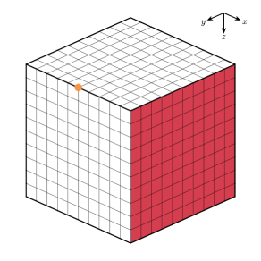
(a) View 1

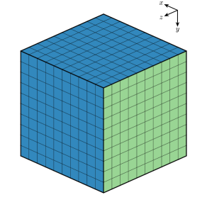
(b) View 2

Figure 2: Cube: Mesh with boundary conditions and node of interest: red denotes applied traction (Neumann boundary condition), blue denotes planar-displacement constraint (Dirichlet boundary condition), green denotes zero-displacement constraint (Dirichlet boundary condition), and orange denotes the node of interest.

This experiment considers $N_{\boldsymbol{\mu}}=3$ parameters. The elastic modulus ${\mu}_{1}=E$ is varied between 75.0 and 125.0 GPa, the Poisson ratio ${\mu}_{2}=\nu$ is varied between 0.200 and 0.350, and the traction ${\mu}_{3}=t$ is varied between 40.0 and 60.0 GPa, resulting in a parameter domain $\mathcal{D}=\left[75.0\,\text{GPa},125.0\,\text{GPa}\right]\times\left[0.200,0.350\right]\times\left[40.0\,\text{GPa},60.0\,\text{GPa}\right]$. Across the parameter domain $\mathcal{D}$, quantities of interest $u_{x}$ and $u_{y}$ vary between limits of 0.242 m and 0.906 m, and $-0.0814$ m and $-0.237$ m, respectively.

To construct the requisite snapshots, we first compute the high-fidelity-model solution $\mathbf{u}(\boldsymbol{\mu})$ for $\boldsymbol{\mu}\in\mathcal{D}_{\mathrm{POD}}\subset\mathcal{D}$, where $\mathcal{D}_{\mathrm{POD}}$ comprises eight Latin hypercube samples such that $M_{\mathbf{u}}=8$. We subsequently compute the trial-basis matrix $\mathbf{\Phi}_{\mathbf{u}}$ using proper orthogonal decomposition (POD) by applying Algorithm 1 of A with inputs $\{\mathbf{u}(\boldsymbol{\mu})\}_{\boldsymbol{\mu}\in\mathcal{D}_{\mathrm{POD}}}$. Due to the simplicity of this problem, the first POD vector captures 95.87% of the statistical energy such that $\upsilon_{1}=0.9587$ (see output of Algorithm 1), and the second captures 3.62% such that $\upsilon_{2}=0.9949\%$. Figure 3 depicts the first two POD basis vectors.

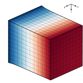
(a) First POD basis vector

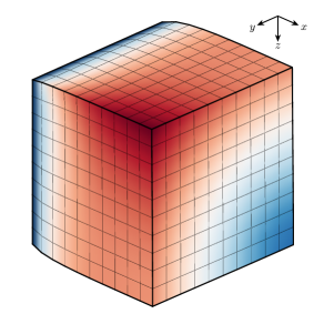
(b) Second POD basis vector

Figure 3: Cube: POD basis vectors. Red indicates larger deformations; blue indicates smaller deformations.

One set of 100 parameter instances is randomly sampled from the parameter domain $\mathcal{D}$ to serve as the set of parameter training instances $\mathcal{D}_{\mathrm{train}}$. To assess method performance for smaller amounts of training data, we randomly create nested training sets from this set. Another set of 100 parameter instances is randomly sampled to serve as the set of parameter testing instances $\mathcal{D}_{\mathrm{test}}$. We consider approximate solutions generated by a Galerkin reduced-order model (i.e., $\mathbf{\Psi}_{\mathbf{u}}=\mathbf{\Phi}_{\mathbf{u}}$) with $\bar{\mathbf{u}}=\mathbf{0}$ using ${N_{\mathrm{approx}}}=2$ different basis dimensions: $m_{\mathbf{u}}^{1}=1$ and $m_{\mathbf{u}}^{2}=2$. We consider both Data Set 1 (pooled) and Data Set 2 (unique) as described in Section 3.3. The former case yields $N_{\mathrm{test}}=200$ testing data points and up to ${N_{\mathrm{train}}}=200$ training points, while the latter yields $N_{\mathrm{test}}=100$ testing points and up to ${N_{\mathrm{train}}}=100$ testing points.

When using Feature-Engineering Methods 7 and 8, three numbers of sample points are used: $n_{{\mathbf{r}}}\in\{10,\,100,\,1000\}$.

4.2.2 Results

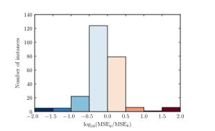
Figure 4: Cube: Comparison of MSE using $k$- and $q$-sampling approaches with $\mathrm{card}\left(\mathcal{D}_{\mathrm{train}}\right)=100$ training parameter instances. When $\text{MSE}_{q}/\text{MSE}_{k}<1$, $q$-sampling outperforms $k$-sampling; these cases are depicted in blue and comprise 61.90% of cases. The converse holds when $\text{MSE}_{q}/\text{MSE}_{k}>1$; these cases are depicted in red and comprise 36.51% of cases. Instances for which $\text{MSE}_{q}=\text{MSE}_{k}$ are not plotted and comprise 1.59% of cases.

We first assess the difference in performance between the $k$- and $q$-sampling approaches for computing the sampling matrix $\mathbf{P}$ employed by Feature-Engineering Methods 7 and 8. Figure 4 provides a comparison of the test MSEs that arise from using $k$- and $q$-sampling with $\mathrm{card}\left(\mathcal{D}_{\mathrm{train}}\right)=100$ parameter training instances. This figure is generated from 252 total data points, which aggregate test MSE values over three errors: $\delta_{{u_{x}}}$, $\delta_{{u_{y}}}$, and $\delta_{\mathbf{u}}$; Feature-Engineering Methods 7 and 8; the seven regression techniques discussed in 3.4; three numbers of sample points $n_{{\mathbf{r}}}\in\{10,100,1000\}$; and the two data-set approaches discussed in Section 3.3. Overall, $q$-sampling outperforms $k$-sampling in this case; therefore, the remaining results for Feature-Engineering Methods 7 and 8 for this experiment consider only $q$-sampling.

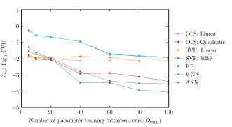
(a) Response = $\delta_{{u_{x}}}$, Data Set 1

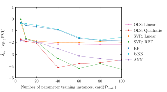
(b) Response = $\delta_{{u_{x}}}$, Data Set 2

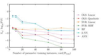
(c) Response = $\delta_{{u_{y}}}$, Data Set 1

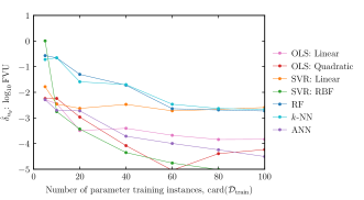
(d) Response = $\delta_{{u_{y}}}$, Data Set 2

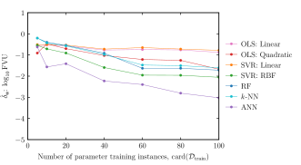
(e) Response = $\delta_{\mathbf{u}}$, Data Set 1

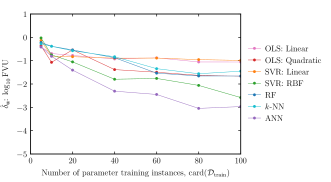
(f) Response = $\delta_{\mathbf{u}}$, Data Set 2

Figure 5: Cube: Comparison of FVU using best feature choice for each ML technique.

For each of the ML regression techniques, Figure 5 reports how the test FVU varies with respect to the number of parameter training instances $\mathrm{card}\left(\mathcal{D}_{\mathrm{train}}\right)$ when using the best-performing feature-engineering method for each regression technique. Generally, as the number of parameter training instances $\mathrm{card}\left(\mathcal{D}_{\mathrm{train}}\right)$ increases, the test FVU decreases, and the best regression techniques are those that enable higher capacity: ANN, SVR: RBF, and OLS: Quadratic. On the other hand, performance of the low-capacity regression methods (OLS: Linear and SVR: Linear) saturates as the amount of training data increases. This saturation can be attributed to the greater structure they enforce, thereby leading to a high bias that produces errors that cannot be reduced with additional training data. Nonetheless, for a small amount of training data, these low-capacity methods perform more competitively, as the higher capacity regression methods overfit the data in this case. RF and $k$-NN exhibit similar performance; they perform poorly with a small amount of training due to their high capacity. Data Set 1 and Data Set 2 perform similarly in this case. Overall, the test FVU values are fairly small, and all techniques work relatively well with a modest number of parameter training instances. Note that predicting $\delta_{\mathbf{u}}$ is more challenging than predicting $\delta_{{u_{x}}}$ or $\delta_{{u_{y}}}$; the low-capacity regression methods (OLS: Linear and SVR: Linear) fail to reduce the test FVU below 0.9 when using Data Set 1 as reported in Figure 5(e).

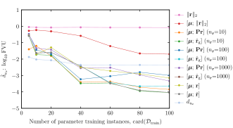
(a) Response = $\delta_{{u_{x}}}$, Data Set 1

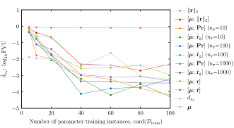
(b) Response = $\delta_{{u_{x}}}$, Data Set 2

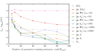
(c) Response = $\delta_{{u_{y}}}$, Data Set 1

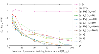
(d) Response = $\delta_{{u_{y}}}$, Data Set 2

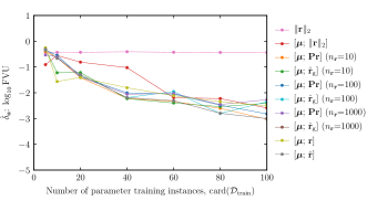
(e) Response = $\delta_{\mathbf{u}}$, Data Set 1

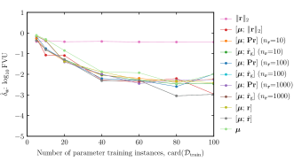
(f) Response = $\delta_{\mathbf{u}}$, Data Set 2

Figure 6: Cube: Comparison of FVU using best ML technique for each feature choice.

Whereas Figure 5 compares each regression technique when using the best feature-engineering method for that technique, Figure 6 compares each feature-engineering method when using the best regression technique for that method. It is immediately clear that using the feature $\|\mathbf{r}\|$ alone yields the highest test FVU, which does not improve as the amount of training data increases. This is expected since $\|\mathbf{r}\|$ is a single feature of relatively low quality. For responses $\delta_{{u_{x}}}$ and $\delta_{{u_{y}}}$, features $d_{u_{x}}$ and $d_{u_{y}}$ tend to perform the best in the presence of limited training data. This is expected since these correspond to single high-quality features. As with Figure 5, predicting $\delta_{\mathbf{u}}$ is more challenging than predicting $\delta_{{u_{x}}}$ or $\delta_{{u_{y}}}$; in this case, the feature-engineering methods perform similarly with the exception of $\|\mathbf{r}\|$. In Figures 6(b) and 6(d), features $[\boldsymbol{\mu};\,\mathbf{P}\mathbf{r}]$ and $[\boldsymbol{\mu};\,\hat{\mathbf{r}}_{\text{g}}]$ typically outperform the commonly used features $\boldsymbol{\mu}$ by roughly an order of magnitude.

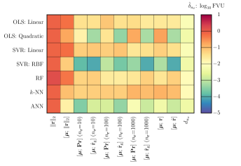
(a) Response = $\delta_{{u_{x}}}$, Data Set 1

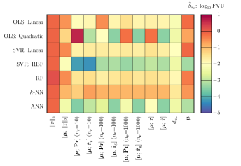
(b) Response = $\delta_{{u_{x}}}$, Data Set 2

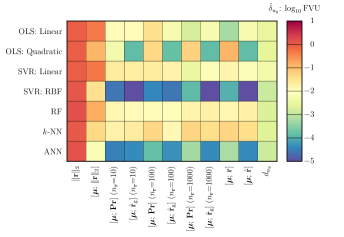
(c) Response = $\delta_{{u_{y}}}$, Data Set 1

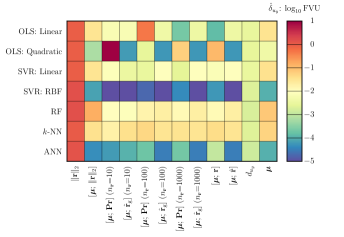
(d) Response = $\delta_{{u_{y}}}$, Data Set 2

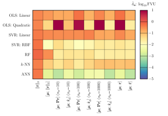
(e) Response = $\delta_{\mathbf{u}}$, Data Set 1

(f) Response = $\delta_{\mathbf{u}}$, Data Set 2

Figure 7: Cube: Comparison of FVU between each ML technique and feature choice with $\mathrm{card}\left(\mathcal{D}_{\mathrm{train}}\right)=100$ training parameter instances.

Figure 7 reports the test FVU for each combination of feature-engineering method, regression technique, and data-set approach for $\mathrm{card}\left(\mathcal{D}_{\mathrm{train}}\right)=100$ parameter training instances. Features $\boldsymbol{\mu}$ require SVR: RBF or ANN to perform well. Regression methods SVR: RBF and ANN consistently yield the best performance, whereas OLS: Quadratic yields very inconsistent performance. Once again, there is not a clear performance discrepancy between the two data-set approaches. Generally, features $[\boldsymbol{\mu};\,\hat{\mathbf{r}}_{\text{g}}]$ perform better than features $[\boldsymbol{\mu};\,\mathbf{P}\mathbf{r}]$; this is particularly clear in Figures 7(a), 7(c), and 7(d). Because features $\|\mathbf{r}\|$, $d_{u_{x}}$, and $d_{u_{y}}$ correspond to only a single feature, their performances are nearly insensitive to the chosen regression technique, as all regression techniques yield similarly low capacities for a small number of features. As demonstrated previously, feature $\|\mathbf{r}\|$ yields large values of the test FVU. For this experiment, full sampling (i.e., $n_{{\mathbf{r}}}=N_{\mathbf{u}}$) and subsampling with $n_{{\mathbf{r}}}=1000$ yield little benefit to significant subsampling with $n_{{\mathbf{r}}}=10$; this implies that excellent performance can be obtained using only a small number of cheaply computable features with the proposed methodology.

For $\mathrm{card}\left(\mathcal{D}_{\mathrm{train}}\right)=100$ parameter training instances, Figure 8 compares the values of the responses $\delta_{{u_{x}}}$, $\delta_{{u_{y}}}$, and $\delta_{\mathbf{u}}$ predicted by various regression methods with their exact values over the test set. The figure reports results for conventional feature choices (i.e., $\|\mathbf{r}\|$; $\boldsymbol{\mu}$; dual-weighted residual, where applicable), as well as $[\boldsymbol{\mu};\,\hat{\mathbf{r}}_{\text{g}}]$ with only $n_{{\mathbf{r}}}=10$ sampled residual elements, where performance of the best regression technique for each of these feature-engineering methods is reported. In each case, $[\boldsymbol{\mu};\,\hat{\mathbf{r}}_{\text{g}}]$ performs better than all conventional approaches, with $r^{2}>0.996$ in every case. We note that although commonly used features $\boldsymbol{\mu}$ with ANN and SVR: RBF regression perform relatively well in this case, this does not occur in subsequent experiments.

Figure 9 assesses the accuracy of the noise model $\hat{\epsilon}\sim\mathcal{N}(0,\hat{\sigma}^{2})$ computed in Step 3 in Section 3.1 for $[\boldsymbol{\mu};\,\hat{\mathbf{r}}_{\text{g}}]$ with $n_{{\mathbf{r}}}=10$ using the best-performing regression technique. In particular, the figure reports the standard normal distribution compared to a histogram of the prediction errors, which have been standardized according to the hypothesized distribution. These prediction errors are computed on a second set of test data ${\mathcal{T}_{\overline{\mathrm{test}}}}\vcentcolon=\{({\delta_{\bar{0},i}},{\mathbf{x}_{\bar{0},i}})\}_{i=1}^{\mathrm{card}\left({\mathcal{T}_{\mathrm{test}}}\right)}$, which is constructed in an identical way to the the first set of test data ${\mathcal{T}_{\mathrm{test}}}$ used to train the noise model, but is independent of ${\mathcal{T}_{\mathrm{test}}}$ and the training data ${\mathcal{T}_{\mathrm{train}}}$ (used to train the regression model). Table 2 lists the corresponding validation frequencies $\omega_{\delta}(\omega)$ for multiple $\omega$-prediction intervals, where

$$\omega_{\delta}(\omega)\vcentcolon=\mathrm{card}\left(\left\{(\delta,\mathbf{x})\in{\mathcal{T}_{\overline{\mathrm{test}}}}\ |\ {(\delta-\hat{f}(\mathbf{x}))}/{\hat{\sigma}^{2}}\in C(\omega)\right\}\right)/\mathrm{card}\left({\mathcal{T}_{\overline{\mathrm{test}}}}\right)$$ (37)

and the standard $\omega$-prediction interval is

$$C(\omega)\vcentcolon=\left[-\sqrt{2}\text{erf}^{-1}(\omega),\,\sqrt{2}\text{erf}^{-1}(\omega)\right].$$ (38)

	$\omega_{\delta}(\omega)$
$\omega$	$\delta_{{u_{x}}}$	$\delta_{{u_{y}}}$	$\delta_{\mathbf{u}}$
0.80	0.96	0.86	0.96
0.90	0.97	0.92	0.97
0.95	0.97	0.93	0.98
0.99	0.98	0.96	0.98

Table 2: Cube: Validation frequencies for models using $[\boldsymbol{\mu};\,\hat{\mathbf{r}}_{\text{g}}]$ ($n_{{\mathbf{r}}}=10$) with SVR: RBF, SVR: RBF, and ANN, respectively for $\delta_{{u_{x}}}$, $\delta_{{u_{y}}}$, and $\delta_{\mathbf{u}}$.

These results show that the data are not quite Gaussian and are characterized by heavier tails than would be predicted by a Gaussian distribution. This motivates the need for a more sophisticated error model to accurately model non-Gaussian noise, which is the subject of future work. However, the validation frequencies show that—while all the prediction intervals of the noise model are not accurate—a subset are accurate. In particular, the 0.99-prediction interval, the 0.95-prediction interval, and the 0.99-prediction interval are reasonably accurate for the models associated with responses $\delta_{{u_{x}}}$, $\delta_{{u_{y}}}$, and $\delta_{\mathbf{u}}$, respectively. Thus, despite the non-Gaussian behavior of the error, these prediction intervals can still be used to make accurate statistical predictions.

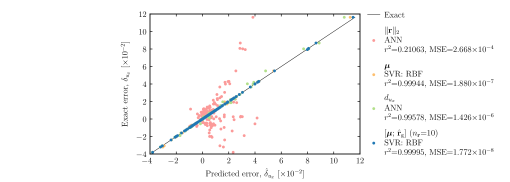
(a) Response = $\delta_{{u_{x}}}$

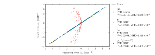
(b) Response = $\delta_{{u_{y}}}$

(c) Response = $\delta_{\mathbf{u}}$

Figure 8: Cube: Comparison of predicted responses, relative to exact.

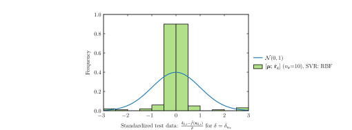
(a) Response = $\delta_{{u_{x}}}$

(b) Response = $\delta_{{u_{y}}}$

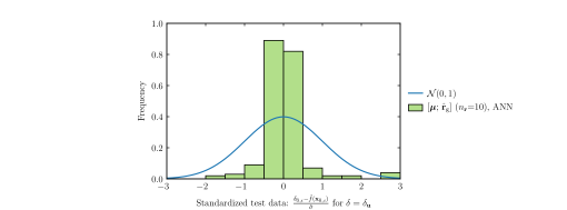
(c) Response = $\delta_{\mathbf{u}}$

Figure 9: Cube: Error in predicted responses for second set of test data, scaled by $\hat{\sigma}^{2}=\text{MSE}$ from the first set of test data.

4.3 PCAP: reduced-order modeling

The second experiment considers the mechanically induced deformation of the Predictive Capability Assessment Project (PCAP) test case with an approximate solution provided by a Galerkin reduced-order model as described in Section 2.1.3. We also conduct this experiment using Albany [74] with eight-node hexahedral elements. We compute solutions with a single nonlinear solve using a damped Newton’s method.

4.3.1 Overview

The PCAP test case is an axisymmetric structure consisting of a tube with different lids attached at each end. The radius of the test case is 4.44 cm, and the height is 6.61 cm. As illustrated in Figure 10, a quarter of the test case is discretized with 77,768 elements and 92,767 nodes.

Pressure is applied as a Neumann boundary condition on the interior of the structure, and the center of the top of the upper lid is further constrained in the $y$-direction. Due to the axisymmetry of the problem, we introduce Dirichlet boundary conditions on the sides to enforce planar displacement. Therefore, the size of the problem is $N_{\mathbf{u}}=274,954$.

We consider two quantities of interest: (1) the $y$-displacement of the center of the top of the bottom lid, denoted by $u_{y}$, and (2) the radial deformation of the outside of the tube, midway along the height, denoted by $u_{r}$. Figure 10 depicts the boundary conditions and nodes of interest.

Figure 10: PCAP: Mesh with boundary conditions and nodes of interest: red denotes applied pressure (Neumann boundary condition), blue denotes planar-displacement constraint (Dirichlet boundary condition), green denotes zero-displacement constraint (Dirichlet boundary condition), and orange denotes nodes of interest.

The lid material has an elastic modulus of 110.3 GPa, a Poisson ratio of 0.32, a yield strength of 88.02 MPa, and a hardening modulus of 232.8 MPa. The tube has a yield strength of 82.94 MPa, and a hardening modulus of 1.088 GPa. This experiment considers $N_{\boldsymbol{\mu}}=3$ parameters. The tube elastic modulus ${\mu}_{1}=E$ is varied between 50.0 and 100.0 GPa, the tube Poisson ratio ${\mu}_{2}=\nu$ is varied between 0.200 and 0.350, and the applied pressure ${\mu}_{3}=p$ is varied between 6.00 and 10.00 GPa. The resulting parameter domain is thus $\mathcal{D}=[50.0\,\text{GPa},100.0\,\text{GPa}]\times[0.200,0.350]\times[6.00\,\text{GPa},10.00\,\text{GPa}]$. Across the parameter domain $\mathcal{D}$, $u_{y}$ varies between limits of $-0.0876$ cm and $-1.04$ cm, which corresponds to 1.3%–15.8% of the undeformed height, and $u_{r}$ varies between limits of 0.185 cm and 0.418 cm, which corresponds to 4.2%–9.4% of the undeformed radius. Figure 11 depicts the test case when undergoing the greatest deformation.

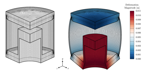
Figure 11: PCAP: Largest simulated deformation (right) compared to undeformed state (left).

To construct the snapshots, we first compute the high-fidelity-model solution $\mathbf{u}(\boldsymbol{\mu})$ for $\boldsymbol{\mu}\in\mathcal{D}_{\mathrm{POD}}\subset\mathcal{D}$, where $\mathcal{D}_{\mathrm{POD}}$ comprises eight Latin hypercube samples such that $M_{\mathbf{u}}=8$. We subsequently compute the trial-basis matrix $\mathbf{\Phi}_{\mathbf{u}}$ using proper orthogonal decomposition (POD) by applying Algorithm 1 of A with inputs $\{\mathbf{u}(\boldsymbol{\mu})\}_{\boldsymbol{\mu}\in\mathcal{D}_{\mathrm{POD}}}$. The relative statistical energy captured by different basis dimensions (see output of Algorithm 1) corresponds to $\upsilon_{1}=0.8503$, $\upsilon_{2}=0.9569$, $\upsilon_{3}=0.9935$, $\upsilon_{4}=0.9977$, $\upsilon_{5}=0.9990$, $\upsilon_{6}=0.9997$, $\upsilon_{7}=0.9999$, and $\upsilon_{8}=1.0000$. Figure 12 illustrates the first five POD basis vectors.

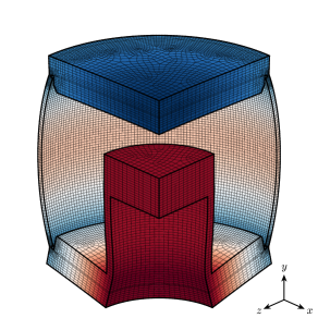
(a) First POD basis vector

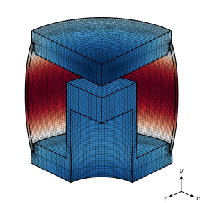
(b) Second POD basis vector

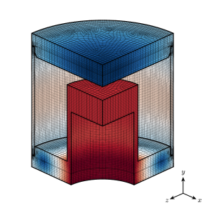
(c) Third POD basis vector

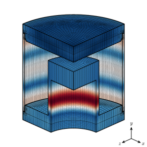
(d) Fourth POD basis vector

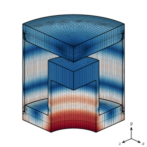
(e) Fifth POD basis vector

Figure 12: PCAP: POD basis vectors. Red indicates largest deformation; blue indicates smallest deformation.

One set of 30 parameter instances is randomly sampled from the parameter domain $\mathcal{D}$ to serve as the set of parameter training instances $\mathcal{D}_{\mathrm{train}}$. To assess method performance for smaller amounts of training data, we randomly create nested training sets from this set. Another set of 30 parameter instances is randomly sampled to serve as the set of parameter testing instances $\mathcal{D}_{\mathrm{test}}$. We consider approximate solutions generated by a Galerkin reduced-order model (i.e., $\mathbf{\Psi}_{\mathbf{u}}=\mathbf{\Phi}_{\mathbf{u}}$) with $\bar{\mathbf{u}}=\mathbf{0}$ using ${N_{\mathrm{approx}}}=5$ different basis dimensions: $m_{\mathbf{u}}^{i}=i$, $i=1,\ldots,5$. We consider both Data Set 1 (pooled) and Data Set 2 (unique) as described in Section 3.3. The former case yields $N_{\mathrm{test}}=150$ testing data points and up to ${N_{\mathrm{train}}}=150$ training points, while the latter yields $N_{\mathrm{test}}=30$ testing points and up to ${N_{\mathrm{train}}}=30$ testing points. We executed the simulations on a workstation with two 2.60-GHz Intel^® Xeon^® E5-2660 v3 processors, which collectively contain 20 logical cores, and 62.8 GB of RAM. Table 3 lists the average and median run times across all training and testing FOM and ROM simulations. For several of the parameter instances, for $m_{\mathbf{u}}^{2}$ and $m_{\mathbf{u}}^{3}$, the nonlinear solver required damping to reduce the step size during the Newton solve in order to converge. For this reason, the average and median times deviate from the monotonically increasing trend among $m_{\mathbf{u}}^{1}$, $m_{\mathbf{u}}^{4}$, and $m_{\mathbf{u}}^{5}$. We note that the ROM yields computational-cost savings in this case—despite the lack of hyper-reduction—due to the low dimensionality of the POD basis.

		Galerkin ROM
	FOM	$m_{\mathbf{u}}^{1}=1$	$m_{\mathbf{u}}^{2}=2$	$m_{\mathbf{u}}^{3}=3$	$m_{\mathbf{u}}^{4}=4$	$m_{\mathbf{u}}^{5}=5$
Average time [seconds]	2208	36.5	182.0	151.6	81.8	93.7
Median time [seconds]	1840	35.5	82.4	108.0	82.4	87.3

Table 3: PCAP: FOM and ROM average and median run times.

The large dimension of this problem renders two feature-engineering methods impractical: Feature-Engineering Method 2, as it requires computing the dual-weighted residual; and Feature-Engineering Method 5, as it employs the entire $N_{\mathbf{u}}$-dimensional residual vector as features. Thus, we do not consider these methods in this set of experiments. When using Feature-Engineering Methods 7 and 8, three sample sizes are used: $n_{{\mathbf{r}}}=\{10,\,100,\,1000\}$.

4.3.2 Results

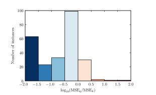
Figure 13: PCAP: Comparison of MSE using $k$- and $q$-sampling approaches with $\mathrm{card}\left(\mathcal{D}_{\mathrm{train}}\right)=30$ training parameter instances. When $\text{MSE}_{q}/\text{MSE}_{k}<1$, $q$-sampling outperforms $k$-sampling; these cases are depicted in blue and comprise 86.51% of cases. The converse holds when $\text{MSE}_{q}/\text{MSE}_{k}>1$; these cases are depicted in red and comprise 13.49% of cases.

Similarly to Section 4.2.2, we first assess the difference in performance between the $k$- and $q$-sampling approaches for computing the sampling matrix $\mathbf{P}$ employed by Feature-Engineering Methods 7 and 8. Figure 13 provides a comparison of the test MSEs that arise from using $k$- and $q$-sampling with $\mathrm{card}\left(\mathcal{D}_{\mathrm{train}}\right)=30$ parameter training instances. This figure is generated from 252 total data points, which aggregate test MSE values over three errors: $\delta_{{u_{r}}}$, $\delta_{{u_{y}}}$, and $\delta_{\mathbf{u}}$; Feature-Engineering Methods 7 and 8; the seven regression techniques discussed in 3.4; three numbers of sample points $n_{{\mathbf{r}}}\in\{10,100,1000\}$; and the two data-set approaches discussed in Section 3.3. In this case, $q$-sampling significantly outperforms $k$-sampling; therefore, the remaining results for this experiment only consider $q$-sampling.

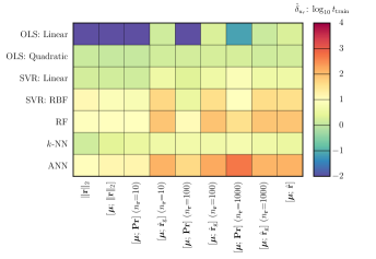
(a) Response = $\delta_{{u_{r}}}$, Data Set 1

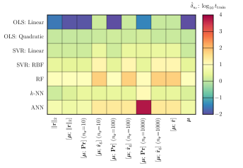
(b) Response = $\delta_{{u_{r}}}$, Data Set 2

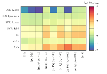
(c) Response = $\delta_{{u_{y}}}$, Data Set 1

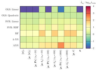
(d) Response = $\delta_{{u_{y}}}$, Data Set 2

(e) Response = $\delta_{\mathbf{u}}$, Data Set 1

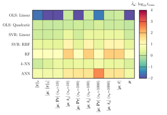
(f) Response = $\delta_{\mathbf{u}}$, Data Set 2

Figure 14: PCAP: Comparison of wall time, in seconds, required to train regression models offline, including cross-validation (Steps 2–9 of Algorithm 3 of B), with $\mathrm{card}\left(\mathcal{D}_{\mathrm{train}}\right)=30$ training parameter instances. After training, all combinations took less than 0.2 seconds to predict during the online stage.

We trained all of the models on a workstation with a 3.60-GHz Intel^® Core^™ i7-4790 processor, which contains eight logical cores, and 16.0 GB of RAM. Figure 14 shows $t_{\text{train}}$, the amount of wall time in seconds it took to train the regression model offline, for each combination of feature-engineering method, regression technique, and data-set approach for $\mathrm{card}\left(\mathcal{D}_{\mathrm{train}}\right)=30$ parameter training instances. This time includes Steps 2–9 of Algorithm 3 of B, which account for cross-validation. As expected, the simplest machine-learning technique, OLS: Linear, required the least amount of time, sometimes less than 16 milliseconds, whereas the most complex, ANN, required the most, as high as 1.64 hours. Additionally, $[\boldsymbol{\mu};\,\mathbf{P}\mathbf{r}]$ with $n_{{\mathbf{r}}}=1000$ required the most amount of time with ANN, due to having the greatest number of features. After training, all combinations took less than 0.2 seconds to predict during the online stage.

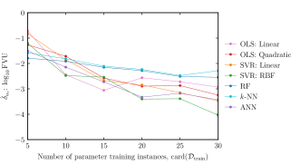
(a) Response = $\delta_{{u_{r}}}$, Data Set 1

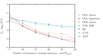
(b) Response = $\delta_{{u_{r}}}$, Data Set 2

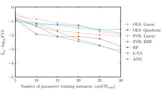
(c) Response = $\delta_{{u_{y}}}$, Data Set 1

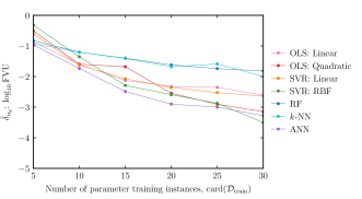
(d) Response = $\delta_{{u_{y}}}$, Data Set 2

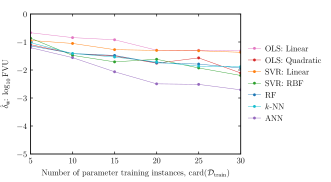
(e) Response = $\delta_{\mathbf{u}}$, Data Set 1

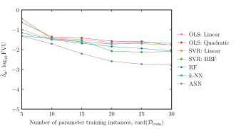
(f) Response = $\delta_{\mathbf{u}}$, Data Set 2

Figure 15: PCAP: Comparison of FVU using best feature choice for each ML technique.

For each of the ML regression techniques, Figure 15 reports how the test FVU varies with respect to the number of parameter training instances $\mathrm{card}\left(\mathcal{D}_{\mathrm{train}}\right)$ when using the best-performing feature-engineering method for each regression technique. Generally, as the number of parameter training instances $\mathrm{card}\left(\mathcal{D}_{\mathrm{train}}\right)$ increases, the test FVU decreases, and the best regression techniques are those that enable higher capacity: ANN and SVR: RBF. In Figures 15(a), 15(b), and 15(d), RF and $k$-NN perform the least competitively, most likely due to an insufficient amount of training data. Data Set 1 and Data Set 2 again perform similarly in this case. Compared to the cube experiments discussed in Section 4.2.2, the test FVU values are noticeably larger in the present experiments, likely due to the greater complexity (i.e., higher solution dimensionality, more complex geometry) of the experiment. Once more, predicting $\delta_{\mathbf{u}}$ is more challenging than predicting $\delta_{{u_{r}}}$ and $\delta_{{u_{y}}}$; in this case, ANN significantly outperforms other regression techniques, as shown in Figures 15(e) and 15(f).

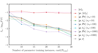
(a) Response = $\delta_{{u_{r}}}$, Data Set 1

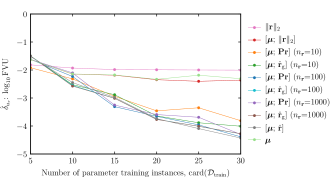
(b) Response = $\delta_{{u_{r}}}$, Data Set 2

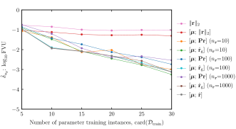
(c) Response = $\delta_{{u_{y}}}$, Data Set 1

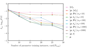
(d) Response = $\delta_{{u_{y}}}$, Data Set 2

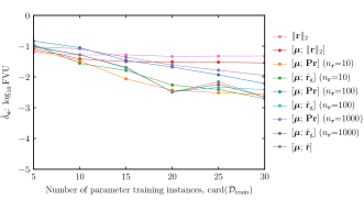
(e) Response = $\delta_{\mathbf{u}}$, Data Set 1

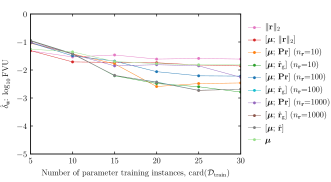
(f) Response = $\delta_{\mathbf{u}}$, Data Set 2

Figure 16: PCAP: Comparison of FVU using best ML technique for each feature choice.

Whereas Figure 15 compares each regression technique when using the best feature-engineering method for that technique, Figure 16 compares each feature-engineering method when using the best regression technique for that method. Once again, it is immediately clear that using the feature $\|\mathbf{r}\|$ alone yields the highest test FVU, which does not improve as the amount of training data increases. Additionally, features $[\boldsymbol{\mu};\,\|\mathbf{r}\|]$ and $\boldsymbol{\mu}$ perform quite poorly, with test FVU values orders of magnitude higher than features $[\boldsymbol{\mu};\,\mathbf{P}\mathbf{r}]$ and $[\boldsymbol{\mu};\,\hat{\mathbf{r}}_{\text{g}}]$. This is a notable result, as employing features $\boldsymbol{\mu}$ is the approach most commonly adopted in the literature (i.e., via the ‘multifidelity correction’ or ‘model discrepancy’ methods).

Figure 17 reports the test FVU for each combination of feature-engineering method, regression technique, and data-set approach for $\mathrm{card}\left(\mathcal{D}_{\mathrm{train}}\right)=30$ parameter training instances. First, we note that SVR: RBF and ANN consistently yield the best performance, whereas OLS: Linear and OLS: Quadratic yield inconsistent performance. In contrast to the cube experiments, Figures 17(a) and 17(b) demonstrate that there is a benefit to training using Data Set 2 rather than Data Set 1. Generally, features $[\boldsymbol{\mu};\,\hat{\mathbf{r}}_{\text{g}}]$ and $[\boldsymbol{\mu};\,\mathbf{P}\mathbf{r}]$ yield similar performance, with $[\boldsymbol{\mu};\,\hat{\mathbf{r}}_{\text{g}}]$ slightly outperforming $[\boldsymbol{\mu};\,\mathbf{P}\mathbf{r}]$ in some cases. Because features $\|\mathbf{r}\|$, $[\boldsymbol{\mu};\,\|\mathbf{r}\|]$, and $\boldsymbol{\mu}$ correspond to a small number of features, their performance is nearly insensitive to regression techniques, as all regression techniques yield similarly low capacities for a small number of features. None of these features yield good performance in this case. We remark that, in this experiment, only $n_{{\mathbf{r}}}=10\ll N_{\mathbf{u}}=278,301$ elements of the residual must be computed to realize coefficients of determination above $r^{2}=0.99$ in all cases with ANN regression; this again implies that excellent performance can be obtained using only a very small number of cheaply computable features with the proposed methodology.

For $\mathrm{card}\left(\mathcal{D}_{\mathrm{train}}\right)=30$ parameter training instances, Figure 18 compares the predicted values of $\delta_{{u_{r}}}$, $\delta_{{u_{y}}}$, and $\delta_{\mathbf{u}}$ with the exact values using the conventional feature choices (i.e., $\|\mathbf{r}\|$, $\boldsymbol{\mu}$), as well as $[\boldsymbol{\mu};\,\hat{\mathbf{r}}_{\text{g}}]$, where performance of the best regression technique for each of these feature-engineering methods is reported. In each case, $[\boldsymbol{\mu};\,\hat{\mathbf{r}}_{\text{g}}]$ performs better than all conventional approaches, with $r^{2}>0.998$ in every case, and with the test MSE reduced by one to two orders of magnitude.

Figure 19 assesses the accuracy of the noise model $\hat{\epsilon}\sim\mathcal{N}(0,\hat{\sigma}^{2})$ computed in Step 3 in Section 3.1 for $[\boldsymbol{\mu};\,\hat{\mathbf{r}}_{\text{g}}]$ with $n_{{\mathbf{r}}}=10$ using the best-performing regression technique. As before, the figure reports the standard normal distribution compared to a histogram of the prediction errors, which have been standardized according to the hypothesized distribution. These prediction errors are computed on a second set of independent test data ${\mathcal{T}_{\overline{\mathrm{test}}}}\vcentcolon=\{({\delta_{\bar{0},i}},{\mathbf{x}_{\bar{0},i}})\}_{i=1}^{\mathrm{card}\left({\mathcal{T}_{\mathrm{test}}}\right)}$, which is constructed in an identical way to the the first set of test data ${\mathcal{T}_{\mathrm{test}}}$. Table 4 lists the corresponding validation frequencies $\omega_{\delta}(\omega)$ (37) for multiple $\omega$-prediction intervals (38).

	$\omega_{\delta}(\omega)$
$\omega$	$\delta_{{u_{r}}}$	$\delta_{{u_{y}}}$	$\delta_{\mathbf{u}}$
0.80	0.8800	0.8133	0.8200
0.90	0.9333	0.9000	0.9133
0.95	0.9400	0.9200	0.9400
0.99	0.9533	0.9667	0.9800

Table 4: PCAP: Validation frequencies for models using $[\boldsymbol{\mu};\,\hat{\mathbf{r}}_{\text{g}}]$ ($n_{{\mathbf{r}}}=10$) with SVR: RBF, ANN, and ANN, respectively for $\delta_{{u_{r}}}$, $\delta_{{u_{y}}}$, and $\delta_{\mathbf{u}}$.

Again, the data are not quite Gaussian, although they appear to match the hypothesized distribution closer than in the cube experiments of Section 4.2. Once more, the tails of the distribution are heavier than what would be predicted by a Gaussian distribution. The table indicates that, despite the data being non-Gaussian, some of the prediction intervals are indeed accurate. Namely, the 0.95-prediction interval; the 0.90-prediction interval; and the 0.90-, 0.95-, and 0.99-prediction intervals are reasonably accurate for the models associated with responses $\delta_{{u_{r}}}$, $\delta_{{u_{y}}}$, and $\delta_{\mathbf{u}}$, respectively.

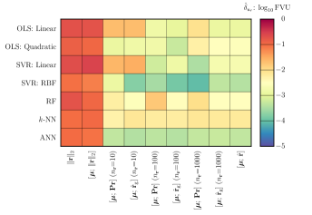
(a) Response = $\delta_{{u_{r}}}$, Data Set 1

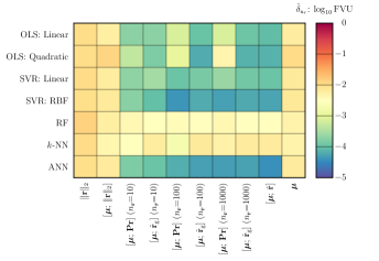
(b) Response = $\delta_{{u_{r}}}$, Data Set 2

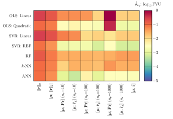
(c) Response = $\delta_{{u_{y}}}$, Data Set 1

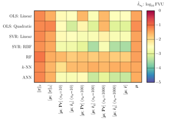
(d) Response = $\delta_{{u_{y}}}$, Data Set 2

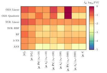
(e) Response = $\delta_{\mathbf{u}}$, Data Set 1

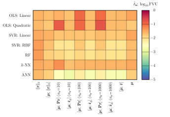
(f) Response = $\delta_{\mathbf{u}}$, Data Set 2

Figure 17: PCAP: Comparison of FVU between each ML technique and feature choice with $\mathrm{card}\left(\mathcal{D}_{\mathrm{train}}\right)=30$ training parameter instances.

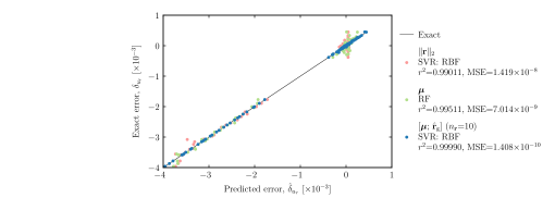
(a) Response = $\delta_{{u_{r}}}$

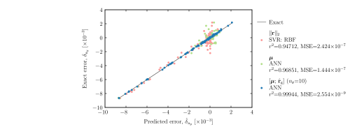
(b) Response = $\delta_{{u_{y}}}$

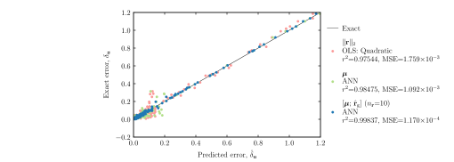
(c) Response = $\delta_{\mathbf{u}}$

Figure 18: PCAP: Comparison of predicted responses, relative to exact.

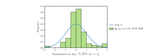
(a) Response = $\delta_{{u_{r}}}$

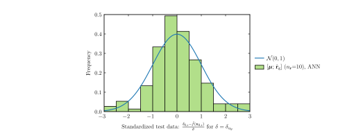
(b) Response = $\delta_{{u_{y}}}$

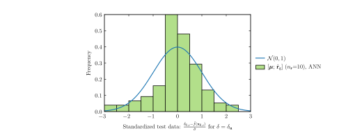
(c) Response = $\delta_{\mathbf{u}}$

Figure 19: PCAP: Error in predicted responses for second set of test data, scaled by $\hat{\sigma}^{2}=\text{MSE}$ from the first set of test data.

4.4 Burgers’ equation: inexact solutions and coarse solution prolongation

The previous two experiments demonstrate the proposed methodology in the context of approximate solutions provided by a Galerkin reduced-order model. Instead, this experiment demonstrates the methodology for two other types of approximate solutions: inexact solutions as described in Section 2.1.1, and lower-fidelity models arising from a coarse mesh as described in Section 2.1.2. We assess these approximate solutions on a forced steady viscous Burgers’ equation.

4.4.1 Overview

We consider the governing equation

$$uu_{x}-\frac{1}{R}u_{xx}=\alpha\sin 2\pi x,$$ (39)

where $x\in[0,\,1]$, $u(0)=u_{a}$ and $u(1)=-u_{a}$. We adopt the finite-difference discretization described in Ref. [75] with $2001$ uniformly spaced nodes, such that $N_{\mathbf{u}}=1999$.

We consider one quantity of interest: the slope $m$ at $x=\frac{1}{2}$ approximated by finite differences as

$$m\vcentcolon=\frac{-u(\frac{1}{2}+2\Delta x)+8u(\frac{1}{2}+\Delta x)-8u(\frac{1}{2}-\Delta x)+u(\frac{1}{2}-2\Delta x)}{12\Delta x},$$

where $\Delta x\equiv 1/(N_{\mathbf{u}}+1)$.

This experiment considers $N_{\boldsymbol{\mu}}=3$ parameters. The source parameter ${\mu}_{1}=\alpha$ varies between 0.10 and 2.00; the boundary-condition magnitude ${\mu}_{2}=u_{a}$ varies between 0.10 and 2.10; and the Reynolds number ${\mu}_{3}=R$ parameter varies between 50 and 1000. Thus, the parameter domain is $\mathcal{D}=[0.10,2.00]\times[0.10,2.10]\times[50,1000]$. Figure 20 depicts the solutions corresponding to the vertices of the hypercube $\mathcal{D}$.

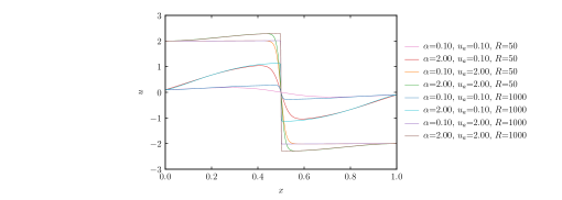
Figure 20: Solutions to Burgers’ equation (39) corresponding to the extrema of $\boldsymbol{\mu}$.

Because this experiment does not employ POD-based reduced-order models, we do not require a snapshot set $\mathcal{D}_{\mathrm{POD}}$. One set of 100 parameter instances is randomly sampled from the parameter domain $\mathcal{D}$ to serve as the set of parameter training instances $\mathcal{D}_{\mathrm{train}}$. To assess method performance for smaller amounts of training data, we randomly create nested training sets from this set. Another set of 100 parameter instances is randomly sampled to serve as the set of parameter testing instances $\mathcal{D}_{\mathrm{test}}$.

For the inexact-solution case, we consider approximate solutions generated by a ${N_{\mathrm{approx}}}=2$ different inexact solutions corresponding to $K=1$ and $K=2$ total Newton iterations applied to solve the governing equations from a linear initial guess $\mathbf{u}^{(0)}$ corresponding to $u(x)=u_{a}(1-2x)$, $x\in[0,1]$. In this case, we consider only Data Set 1 (pooled) as described in Section 3.3, yielding $N_{\mathrm{test}}=100$ testing points and up to ${N_{\mathrm{train}}}=100$ testing points.

For the lower-fidelity-model case, we consider approximate solutions generated from ${N_{\mathrm{approx}}}=2$ different coarse meshes, corresponding to $N_{\mathbf{u}_{\text{LF}}}=499$ and $N_{\mathbf{u}_{\text{LF}}}=999$; each of these cases employs the same discretization as the high-fidelity model and an equispaced grid. In this case, we consider both Data Set 1 (pooled) and Data Set 2 (unique) as described in Section 3.3. The former case yields $N_{\mathrm{test}}=200$ testing data points and up to ${N_{\mathrm{train}}}=200$ training points, while the latter yields $N_{\mathrm{test}}=100$ testing points and up to ${N_{\mathrm{train}}}=100$ testing points. When using Feature-Engineering Methods 7 and 8, three sample sizes are used: $n_{{\mathbf{r}}}=\{10,\,100,\,1000\}$.

4.4.2 Results: inexact solutions

Again, we first assess the difference in performance between the $k$- and $q$-sampling approaches for computing the sampling matrix $\mathbf{P}$ employed by Feature-Engineering Methods 7 and 8. Figure 21 provides a comparison of the test MSEs that arise from using $k$- and $q$-sampling with $\mathrm{card}\left(\mathcal{D}_{\mathrm{train}}\right)=100$ training runs. This figure is generated from 42 total data points, which aggregate test MSE values over Feature-Engineering Methods 7 and 8, the seven regression techniques discussed in 3.4, and three numbers of sample points $n_{{\mathbf{r}}}\in\{10,100,1000\}$. Yet again, $q$-sampling significantly outperforms $k$-sampling; therefore, the remaining results for this experiment only consider $q$-sampling.

For each of the ML regression techniques, Figure 22 reports how the test FVU varies with respect to the number of parameter training instances $\mathrm{card}\left(\mathcal{D}_{\mathrm{train}}\right)$. Consistent with observations in previous experiments, as the number of parameter training instances $\mathrm{card}\left(\mathcal{D}_{\mathrm{train}}\right)$ increases, the test FVU decreases, and the best regression techniques are those that enable higher capacity: ANN and SVR: RBF. In this case, these two regression techniques yield roughly two orders of magnitude smaller test FVU values than other regression techniques for $\mathrm{card}\left(\mathcal{D}_{\mathrm{train}}\right)=100$ training runs. The two linear methods OLS: Linear and SVR: Linear are unable to reduce the test FVU below 0.1 (with any feature choice), even with a large amount of training data, due to their relatively low capacity.

Figure 23 compares each feature-engineering method when using the best regression technique for that method. Once again, it is clear that using the feature $\|\mathbf{r}\|$ alone yields the highest test FVU, which does not improve as the amount of training data increases. Generally, using features $[\boldsymbol{\mu};\,\hat{\mathbf{r}}_{\text{g}}]$ yields better performance than using features $[\boldsymbol{\mu};\,\mathbf{P}\mathbf{r}]$.

Figure 24 reports the test FVU for each combination of feature-engineering method and regression technique for $\mathrm{card}\left(\mathcal{D}_{\mathrm{train}}\right)=100$ parameter training instances. First, we note that SVR: RBF and ANN again consistently yield the best performance, while OLS: Linear and OLS: Quadratic yield inconsistent performance. Furthermore, it is apparent that features $[\boldsymbol{\mu};\,\hat{\mathbf{r}}_{\text{g}}]$ yield significantly better performance than features $[\boldsymbol{\mu};\,\mathbf{P}\mathbf{r}]$, despite the fact they employ the same underlying samples of the residual vector. For this experiment, a remarkably small number of residual samples $n_{{\mathbf{r}}}=10$ is required to yield a coefficient of determination $r^{2}$ exceeding 0.999; this is achieved for features $[\boldsymbol{\mu};\,\hat{{\mathbf{r}}}_{\mathrm{g}}(\boldsymbol{\mu})]$ and ANN regression.

For $\mathrm{card}\left(\mathcal{D}_{\mathrm{train}}\right)=100$ parameter training instances, Figure 25 compares the predicted values of $e_{m}$ with the exact values using the conventional feature choice $\|\mathbf{r}\|$, as well as features $[\boldsymbol{\mu};\,\hat{\mathbf{r}}_{\text{g}}]$, each with their best-performing regression technique. Features $[\boldsymbol{\mu};\,\hat{\mathbf{r}}_{\text{g}}]$ yield drastically better performance than the conventional choice in this case, as it yields a coefficient of determination $r^{2}$ exceeding $0.9999$ and a test MSE that is several orders of magnitude smaller than that obtained with the conventional feature choice. We emphasize that the conventional approach in this case yields a poor coefficient of determination $r^{2}=0.26913$.

Figure 26 assesses the accuracy of the noise model $\hat{\epsilon}\sim\mathcal{N}(0,\hat{\sigma}^{2})$ computed in Step 3 in Section 3.1 for $[\boldsymbol{\mu};\,\hat{\mathbf{r}}_{\text{g}}]$ with $n_{{\mathbf{r}}}=10$ using the best-performing regression technique. As before, the figure reports the standard normal distribution compared to a histogram of the prediction errors, which have been standardized according to the hypothesized distribution. These prediction errors are computed on a second set of independent test data ${\mathcal{T}_{\overline{\mathrm{test}}}}\vcentcolon=\{({\delta_{\bar{0},i}},{\mathbf{x}_{\bar{0},i}})\}_{i=1}^{\mathrm{card}\left({\mathcal{T}_{\mathrm{test}}}\right)}$, which is constructed in an identical way to the the first set of test data ${\mathcal{T}_{\mathrm{test}}}$. Table 5 lists the corresponding validation frequencies $\omega_{\delta_{{m}}}(\omega)$ (37) for multiple $\omega$-prediction intervals (38).

$\omega$	$\omega_{\delta_{{m}}}(\omega)$
0.80	0.830
0.90	0.900
0.95	0.940
0.99	0.970

Table 5: Inexact solutions: Validation frequencies for model using $[\boldsymbol{\mu};\,\hat{\mathbf{r}}_{\text{g}}]$ ($n_{{\mathbf{r}}}=10$) with ANN.

In this case, the data appear to be relatively close to Gaussian. This is further evidenced by the accuracy of the 0.90- and 0.95-prediction intervals.

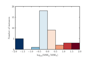
Figure 21: Inexact solutions: Comparison of MSE using $k$- and $q$-sampling approaches with $\mathrm{card}\left(\mathcal{D}_{\mathrm{train}}\right)=100$ training parameter instances. When $\text{MSE}_{q}/\text{MSE}_{k}<1$, $q$-sampling outperforms $k$-sampling; these cases are depicted in blue and comprise 57.14% of cases. The converse holds when $\text{MSE}_{q}/\text{MSE}_{k}>1$; these cases are depicted in red and comprise 40.48% of cases. Instances for which $\text{MSE}_{q}=\text{MSE}_{k}$ are not plotted and comprise 2.38% of cases.

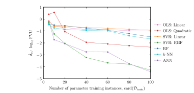
(a) Response = $\delta_{{m}}$, Data Set 1

Figure 22: Inexact solutions: Comparison of FVU using best feature choice for each ML technique.

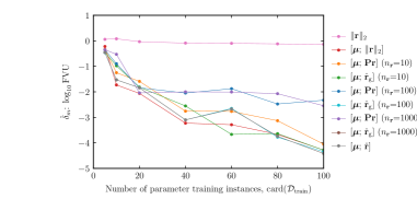
(a) Response = $\delta_{{m}}$, Data Set 1

Figure 23: Inexact solutions: Comparison of FVU using best ML technique for each feature choice.

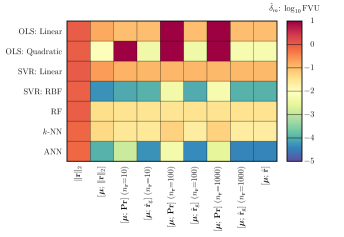
(a) Response = $\delta_{{m}}$, Data Set 1

Figure 24: Inexact solutions: Comparison of FVU between each ML technique and feature choice with $\mathrm{card}\left(\mathcal{D}_{\mathrm{train}}\right)=100$ training parameter instances.

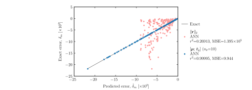
(a) Response = $\delta_{{m}}$

Figure 25: Inexact solutions: Comparison of predicted responses, relative to exact.

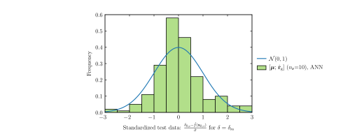
(a) Response = $\delta_{{m}}$

Figure 26: Inexact solutions: Error in predicted responses for second set of test data, scaled by $\hat{\sigma}^{2}=\text{MSE}$ from the first set of test data.

4.4.3 Results: coarse solution prolongation

We again assess the difference in performance between the $k$- and $q$-sampling approaches. Figure 27 provides a comparison of the test MSEs that arise from using $k$- and $q$-sampling with $\mathrm{card}\left(\mathcal{D}_{\mathrm{train}}\right)=100$ parameter training instances. The 84 data points aggregate test MSE values over Feature-Engineering Methods 7 and 8, the seven regression techniques discussed in 3.4, three numbers of sample points $n_{{\mathbf{r}}}\in\{10,100,1000\}$, and the two data-set approaches discussed in Section 3.3. Once more, $q$-sampling outperforms $k$-sampling; therefore, the remaining results for this experiment only consider $q$-sampling.

For each of the ML regression techniques, Figure 28 reports how the test FVU varies with respect to the number of parameter training instances $\mathrm{card}\left(\mathcal{D}_{\mathrm{train}}\right)$. Again, the test FVU decreases as the number of parameter training instances $\mathrm{card}\left(\mathcal{D}_{\mathrm{train}}\right)$ increases, and the best regression techniques are those that enable higher capacity: ANN and SVR: RBF. In addition, OLS: Quadratic performs relatively well, although its performance is highly sensitive to the feature choice as shown in Figure 30. RF and $k$-NN yield the worst performance, most likely due to an insufficient amount of training data.

Figure 29 compares each feature-engineering method when using the best regression technique for that method. Yet again, using the feature $\|\mathbf{r}\|$ alone yields the highest test FVU, which does not improve as the amount of training data increases. Generally, using features $[\boldsymbol{\mu};\,\hat{\mathbf{r}}_{\text{g}}]$ or $[\boldsymbol{\mu};\,\hat{\mathbf{r}}]$ typically yields better performance that using commonly used features $\boldsymbol{\mu}$. Additionally, in this case, employing Data Set 2 yields significantly better performance than employing Data Set 1. This implies that the feature–error relationship is quite different between the two coarse meshes considered. As a result, constructing a regression model from the union of their respective data results in relatively poor performance—even with access to twice as much training data—compared with regression models trained on each coarse-mesh model independently (see discussion of Data Set 1 in Section 3.3).

Figure 30 reports the test FVU for each combination of feature-engineering method, regression technique, and data-set approach for $\mathrm{card}\left(\mathcal{D}_{\mathrm{train}}\right)=100$ parameter training instances. Again, we observe the best performance from regression techniques SVR: RBF and ANN. This figure again illustrates the benefit to employing Data Set 2 rather than Data Set 1. Again, we observe superior performance from features $[\boldsymbol{\mu};\,\hat{\mathbf{r}}_{\text{g}}]$ compared with features $[\boldsymbol{\mu};\,\mathbf{P}\mathbf{r}]$, even though they use the same sampled elements of the residual. As previously observed, feature $\|\mathbf{r}\|$ is nearly insensitive to regression technique and yields relatively poor performance, as it corresponds to a single low-quality feature. We observe that only $n_{{\mathbf{r}}}=10$ samples are needed to achieve a coefficient of determination $r^{2}$ exceeding $0.9999$, which is achieved for $[\boldsymbol{\mu};\,\hat{{\mathbf{r}}}_{\mathrm{g}}(\boldsymbol{\mu})]$ and SVR: RBF regression using Data Set 2.

For $\mathrm{card}\left(\mathcal{D}_{\mathrm{train}}\right)=100$ parameter training instances, Figure 31 compares the predicted values of $e_{m}$ with the exact values using the conventional feature choices: $\|\mathbf{r}\|$ and $\boldsymbol{\mu}$, as well as $[\boldsymbol{\mu};\,\hat{\mathbf{r}}_{\text{g}}]$, where performance of the best regression technique for each of these feature-engineering methods is reported. Features $[\boldsymbol{\mu};\,\hat{\mathbf{r}}_{\text{g}}]$ perform better than conventional features, yielding test MSE values whose values are one to two orders of magnitude lower.

Figure 32 assesses the accuracy of the noise model $\hat{\epsilon}\sim\mathcal{N}(0,\hat{\sigma}^{2})$ computed in Step 3 in Section 3.1 for $[\boldsymbol{\mu};\,\hat{\mathbf{r}}_{\text{g}}]$ with $n_{{\mathbf{r}}}=10$ using the best-performing regression technique. As before, the figure reports the standard normal distribution compared to a histogram of the prediction errors, which have been standardized according to the hypothesized distribution. These prediction errors are computed on a second set of independent test data ${\mathcal{T}_{\overline{\mathrm{test}}}}\vcentcolon=\{({\delta_{\bar{0},i}},{\mathbf{x}_{\bar{0},i}})\}_{i=1}^{\mathrm{card}\left({\mathcal{T}_{\mathrm{test}}}\right)}$, which is constructed in an identical way to the the first set of test data ${\mathcal{T}_{\mathrm{test}}}$. Table 6 lists the corresponding validation frequencies $\omega_{\delta_{{m}}}(\omega)$ (37) for multiple $\omega$-prediction intervals (38).

$\omega$	$\omega_{\delta_{{m}}}(\omega)$
0.80	0.935
0.90	0.950
0.95	0.965
0.99	0.970

Table 6: Coarse solution prolongation: Validation frequencies for model using $[\boldsymbol{\mu};\,\hat{\mathbf{r}}_{\text{g}}]$ ($n_{{\mathbf{r}}}=10$) with SVR: RBF.

Here, the data appear to be somewhat close to Gaussian, as evidenced by the accuracy of the 0.95- and 0.99-prediction intervals. Nonetheless, future work entails construction of more sophisticated noise models to more accurately capture non-Gaussian or heteroscedastic behavior.

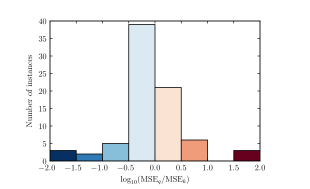
Figure 27: Coarse solution prolongation: Comparison of MSE using $k$- and $q$-sampling approaches with $\mathrm{card}\left(\mathcal{D}_{\mathrm{train}}\right)=100$ training parameter instances. When $\text{MSE}_{q}/\text{MSE}_{k}<1$, $q$-sampling outperforms $k$-sampling; these cases are depicted in blue and comprise 58.33% of cases. The converse holds when $\text{MSE}_{q}/\text{MSE}_{k}>1$; these cases are depicted in red and comprise 35.71% of cases. Instances for which $\text{MSE}_{q}=\text{MSE}_{k}$ are not plotted and comprise 5.95% of cases.

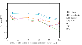
(a) Response = $\delta_{{m}}$, Data Set 1

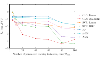
(b) Response = $\delta_{{m}}$, Data Set 2

Figure 28: Coarse solution prolongation: Comparison of FVU using best feature choice for each ML technique.

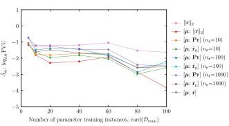
(a) Response = $\delta_{{m}}$, Data Set 1

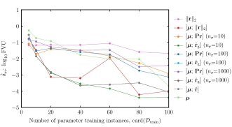
(b) Response = $\delta_{{m}}$, Data Set 2

Figure 29: Coarse solution prolongation: Comparison of FVU using best ML technique for each feature choice.

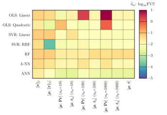
(a) Response = $\delta_{{m}}$, Data Set 1

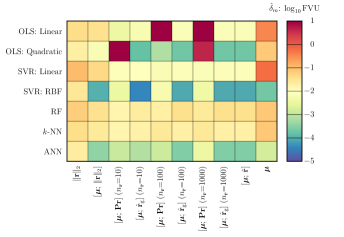
(b) Response = $\delta_{{m}}$, Data Set 2

Figure 30: Coarse solution prolongation: Comparison of FVU between each ML technique and feature choice with $\mathrm{card}\left(\mathcal{D}_{\mathrm{train}}\right)=100$ training parameter instances.

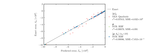
(a) Response = $\delta_{{m}}$

Figure 31: Coarse solution prolongation: Comparison of predicted responses, relative to exact.

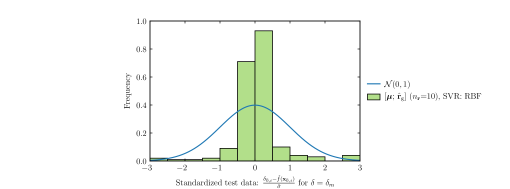
(a) Response = $\delta_{{m}}$

Figure 32: Coarse solution prolongation: Error in predicted responses for second set of test data, scaled by $\hat{\sigma}^{2}=\text{MSE}$ from the first set of test data.

4.5 Summary

We now summarize the dominant trends observed in the numerical experiments reported in Sections 4.2–4.4.

4.5.1 Feature-engineering methods

First, Feature-Engineering Method 1, which employs features $\boldsymbol{\mu}$, is the most commonly adopted technique in the literature. The numerical experiments observe that this technique yields good performance only if applied with regression methods SVR: RBF or ANN; it performs poorly with the standard technique OLS: Linear. Furthermore, this feature-engineering method is always outperformed by one of the new feature-engineering methods proposed in this work. Second, we observe that Feature-Engineering Method 2, which employs dual-weighted-residual features $d(\boldsymbol{\mu})$ and was employed by the ROMES method [38], yields fairly good performance for a small training set, as it is a single high-quality feature. However, it is costly to compute, as it requires a dual solve, and is not practical for application to large-scale problems. Third, we observe that Feature-Engineering Method 4, which employs features $\|{\mathbf{r}}(\boldsymbol{\mu})\|$, yields poor performance, as it comprises a single low-quality feature. Additionally, its computation incurs an $N_{\mathbf{u}}$-dependent operation count. Ultimately, the best-performing feature-engineering technique is Feature-Engineering Method 7, which is newly proposed in this work and employs features $[\boldsymbol{\mu};\,\hat{{\mathbf{r}}}_{\mathrm{g}}(\boldsymbol{\mu})]$; this approach yields a coefficient of determination $r^{2}$ in excess of $0.996$ in each experiment. Moreover, these features can be computed inexpensively, as they require computing only a small number of residual elements. In many cases, sampling only 10 elements of the residual is sufficient to produce very accurate regression models with low-noise-variance results, and there is rarely much benefit to using more than 100 residual samples.

We additionally observe that for Feature-Engineering Methods 7 and 8, the best approach for computing the required sampling matrix $\mathbf{P}$ is the q-sampling approach proposed in the model-reduction community [67]; this technique consistently outperforms k-sampling, which is a linear univariate feature selection approach developed in the machine-learning community. This result is of interest, as it is one of the first examples of a technique developed in the model-reduction community improving the performance of standard machine-learning methods.

4.5.2 Regression techniques

Overall, we observe that low-capacity linear regression methods OLS: Linear and SVR: Linear tend to yield relatively poor performance that does not significantly improve as the amount of training data increases. We also observe that RF and $k$-NN tend to yield the worst performance, as these high-capacity regression methods likely require more data to generalize well. Due to the strong structure imposed by OLS: Linear and OLS: Quadratic techniques, the performance of these methods is highly dependent on the choice of features; in particular, Feature-Engineering Method 7 produces significantly better performance for these regression techniques than does Feature-Engineering Method 8, despite their reliance on the same sampled elements of the residual. Consistently, regression methods SVR: RBF and ANN yield the best performance. Overall, the best results are typically obtained with these two regression techniques and Feature-Engineering Method 7 deployed with a relatively small number of residual samples.

4.5.3 Data-set construction methods

Overall, Data Set 1 and Data Set 2 lead to similar performance, with Data Set 2 performing slightly better. Data Set 1 provides the advantage of more training data per high-fidelity solution; however, this advantage appears to be undermined by the disparity in error magnitudes across the different approximation solutions (e.g., $m_{\mathbf{u}}$, $K$, or $N_{\mathbf{u}_{\text{LF}}}$).

5 Conclusions

This work has proposed a novel approach for quantifying both quantity-of-interest errors and normed solution errors in approximate solutions to parameterized systems of nonlinear equations. The technique applies machine-learning regression methods (e.g., support vector regression, artificial neural networks) to map features (i.e., error indicators such as residual gappy principal components) to a prediction of the error; the noise model quantifies the epistemic uncertainty introduced by the approximate solution and is modeled as a mean-zero, constant-variance Gaussian random variable whose variance corresponds to the sample variance of the approximate-solution error on a test set.

Experiments conducted on a range of computational-mechanics problems and types of approximate solutions demonstrated that the best performance overall was obtained by Feature-Engineering Method 7, which employs features $[\boldsymbol{\mu};\,\hat{{\mathbf{r}}}_{\mathrm{g}}(\boldsymbol{\mu})]$, and regression techniques corresponding to support vector regression with a Gaussian radial-basis-function kernel (SVR: RBF) and a feed-forward artificial neural network (ANN). It is important to note that, even for problems with a quarter of a million degrees of freedom, the proposed method is able to generate inexpensive-to-evaluate machine-learning error models exhibiting coefficients of determination exceeding $r^{2}=0.996$; computing the features required for the error model necessitated evaluating only ten elements of the residual vector.

Future work involves extending the methodology to dynamical systems, developing higher-capacity heteroscedastic noise models, and deploying the methodology on approximate solutions to coupled systems.

Appendix A POD algorithm

Algorithm 1 reports the POD algorithm considered in this work.

Algorithm 1 Proper orthogonal decomposition

0:  Snapshots $\{\mathbf{u}^{i}\}_{i=1}^{M_{\mathbf{u}}}\subset\mathbb{R}^{N_{\mathbf{u}}}$

0:  (Full) POD basis $\mathbf{\Phi}_{\mathbf{u}}\in\mathbb{R}_{\star}^{N_{\mathbf{u}}\times M_{\mathbf{u}}}$; statistical energy captured by different basis dimensions $\upsilon_{i}$, $i=1,\ldots,M_{\mathbf{u}}$

1:  Compute singular value decomposition $[\mathbf{u}^{1}\ \cdots\ \mathbf{u}^{M_{\mathbf{u}}}]=\bar{\mathbf{U}}\bar{\boldsymbol{\Sigma}}\bar{\mathbf{V}}^{T}$ with $\bar{\mathbf{U}}\equiv[\bar{\mathbf{u}}_{1}\ \cdots\ \bar{\mathbf{u}}_{M_{\mathbf{u}}}]$, $\bar{\mathbf{V}}\equiv[\bar{\mathbf{v}}_{1}\ \cdots\ \bar{\mathbf{v}}_{M_{\mathbf{u}}}]$, and $\bar{\boldsymbol{\Sigma}}\equiv\mathrm{diag}(\bar{{\sigma}}_{i})$ and $\bar{{\sigma}}_{1}\geq\cdots\geq\bar{{\sigma}}_{M_{\mathbf{u}}}\geq 0$.

2:  Determine statistical energy captured by different basis dimensions: $\upsilon_{i}=\sum_{k=1}^{i}\bar{{\sigma}}_{k}^{2}/\sum_{k=1}^{M_{\mathbf{u}}}\bar{{\sigma}}_{k}^{2}$, $i=1,\ldots,M_{\mathbf{u}}$.

Appendix B Method algorithms

This section provides the algorithms employed by the proposed method. The offline stage executes Algorithm 2, followed by Algorithm 3. The online stage executes Algorithm 4.

Algorithm 2 Offline stage, step 1: data generation

0:  Parameter training instances $\mathcal{D}_{\mathrm{train}}\subset\mathcal{D}$, parameter test instances $\mathcal{D}_{\mathrm{test}}\subset\mathcal{D}$, number of different types of approximate solutions ${N_{\mathrm{approx}}}\geq 1$, error of interest $\delta\in\{\delta_{s},\delta_{\mathbf{u}}\}$, feature-engineering method (see Section 3.2), data-set method (see Section 3.3)

0:  Training data ${\mathcal{T}_{\mathrm{train}}}$, test data ${\mathcal{T}_{\mathrm{test}}}$, training data for residual PCA $\mathcal{T}_{\mathrm{train},{\mathbf{r}}}$ (if Feature-Engineering Method 6 or 7 is selected)

1:  for $\boldsymbol{\mu}\in\mathcal{D}_{\mathrm{train}}\cup\mathcal{D}_{\mathrm{test}}$ do

2:     Compute the state $\mathbf{u}(\boldsymbol{\mu})$ by solving Eq. (1).

3:     for $i=1,\ldots,{N_{\mathrm{approx}}}$ do

4:        Compute the $i$th approximate solution $\tilde{\mathbf{u}}^{i}(\boldsymbol{\mu})$.

5:        Compute the error

$$\delta^{i}(\boldsymbol{\mu})=\left\{\begin{array}[]{@{} c l @{}}g(\mathbf{u}(\boldsymbol{\mu}))-g(\tilde{\mathbf{u}}^{i}(\boldsymbol{\mu})),&\text{if}\ \delta=\delta_{s}\\[5.0pt] \|\mathbf{u}(\boldsymbol{\mu})-\tilde{\mathbf{u}}^{i}(\boldsymbol{\mu})\|,&\text{if}\ \delta=\delta_{\mathbf{u}}\end{array}\right..$$

6:     end for

7:  end for

8:  if Feature-Engineering Method 6 or 7 is selected then

9:     for $\boldsymbol{\mu}\in\mathcal{D}_{\mathrm{train}}$ do

10:        for $i=1,\ldots,{N_{\mathrm{approx}}}$ do

11:           Compute the residual $\mathbf{r}(\tilde{\mathbf{u}}^{i}(\boldsymbol{\mu});\boldsymbol{\mu})$.

12:        end for

13:     end for

14:     Define the training data for residual PCA $\mathcal{T}_{\mathrm{train},{\mathbf{r}}}$ according to Eq. (26) if Data Set 1 is selected, or according to Eq. (27) if Data Set 2 is selected.

15:     Compute the residual-principal-component matrix $\mathbf{\Phi}_{\mathbf{r}}$ from the training data $\mathcal{T}_{\mathrm{train},{\mathbf{r}}}$.

16:  end if

17:  for $\boldsymbol{\mu}\in\mathcal{D}_{\mathrm{train}}\cup\mathcal{D}_{\mathrm{test}}$ do

18:     for $i=1,\ldots,{N_{\mathrm{approx}}}$ do

19:        Compute the features $\mathbf{x}^{i}(\boldsymbol{\mu})$ resulting from the $i$th approximate solution $\tilde{\mathbf{u}}^{i}(\boldsymbol{\mu})$.

20:     end for

21:  end for

22:  Define the training data ${\mathcal{T}_{\mathrm{train}}}$ and test data ${\mathcal{T}_{\mathrm{test}}}$ according to Eq. (24) if Data Set 1 is selected, or according to Eq. (25) if Data Set 2 is selected.

Algorithm 3 Offline stage, step 2: construction of regression and noise models

0:  Training data ${\mathcal{T}_{\mathrm{train}}}$, test data ${\mathcal{T}_{\mathrm{test}}}\vcentcolon=\{({\delta_{0,i}},{\mathbf{x}_{0,i}})\}_{i=1}^{N_{\mathrm{test}}}$, number of cross-validation folds $k$, regression model (see Section 3.4), regression-model hyperparameters ${\boldsymbol{\theta}}$, cross-validation grid ${\boldsymbol{\Theta}}$

0:  Regression model $\hat{f}$, noise-model variance $\hat{\sigma}^{2}$

1:  Randomly divide the training data into $k$ non-overlapping sets ${\mathcal{T}_{\mathrm{train}}^{i}}\vcentcolon=\{(\delta_{i,\ell},\mathbf{x}_{i,\ell})\}_{\ell}\subset{\mathcal{T}_{\mathrm{train}}}$, $i=1,\ldots,k$ such that ${\mathcal{T}_{\mathrm{train}}^{i}}\cap{\mathcal{T}_{\mathrm{train}}^{j}}=\emptyset$ for $i\neq j$ and $\cup_{i=1}^{k}{\mathcal{T}_{\mathrm{train}}^{i}}={\mathcal{T}_{\mathrm{train}}}$.

2:  for $i=1,\ldots,k$ do

3:     for ${\boldsymbol{\theta}}\in{\boldsymbol{\Theta}}$ do

4:        Compute the regression model $\hat{f}_{i,{\boldsymbol{\theta}}}$ using training set $\cup_{j\in\{1,\ldots,k\}\setminus i}{\mathcal{T}_{\mathrm{train}}^{j}}$ and hyperparameters ${\boldsymbol{\theta}}$.

5:        Compute the mean-squared-error cross-validation loss $L_{i,{\boldsymbol{\theta}}}=\frac{1}{\mathrm{card}\left({\mathcal{T}_{\mathrm{train}}^{i}}\right)}\sum_{\ell=1}^{\mathrm{card}\left({\mathcal{T}_{\mathrm{train}}^{i}}\right)}(\delta_{i,\ell}-\hat{f}_{i,{\boldsymbol{\theta}}}(\mathbf{x}_{i,\ell}))^{2}$.

6:     end for

7:  end for

8:  Select hyperparameters ${\boldsymbol{\theta}}^{\star}=\arg\min_{{\boldsymbol{\theta}}\in{\boldsymbol{\Theta}}}\sum_{i=1}^{k}L_{i,{\boldsymbol{\theta}}}$.

9:  Compute regression model $\hat{f}$ using the full training set ${\mathcal{T}_{\mathrm{train}}}$ and hyperparameters ${\boldsymbol{\theta}}^{\star}$.

10:  Compute the noise-model variance as the mean-squared-error test loss $\hat{\sigma}^{2}=\frac{1}{N_{\mathrm{test}}}\sum_{i=1}^{N_{\mathrm{test}}}({\delta_{0,i}}-\hat{f}({\mathbf{x}_{0,i}}))^{2}$.

Algorithm 4 Online stage

0:  Online parameter instance $\boldsymbol{\mu}\in\mathcal{D}$, regression model $\hat{f}$, noise-model variance $\hat{\sigma}^{2}$

0:  Approximate solution $\tilde{\mathbf{u}}(\boldsymbol{\mu})$, quantity-of-interest approximation $\tilde{s}(\boldsymbol{\mu})$, error-model prediction $\hat{\delta}(\boldsymbol{\mu})$

1:  Compute the approximate solution $\tilde{\mathbf{u}}(\boldsymbol{\mu})$, quantity-of-interest approximation $\tilde{s}(\boldsymbol{\mu})\vcentcolon=g(\tilde{\mathbf{u}}(\boldsymbol{\mu}))$, and resulting features $\mathbf{x}(\boldsymbol{\mu})$.

2:  Compute the error-model prediction $\hat{\delta}(\boldsymbol{\mu})=\hat{f}(\mathbf{x}(\boldsymbol{\mu}))+\hat{\epsilon}$ with $\hat{\epsilon}\sim\mathcal{N}(0,\hat{\sigma}^{2})$.

References

- [1] T. Bui-Thanh, K. Willcox, O. Ghattas, Parametric reduced-order models for probabilistic analysis of unsteady aerodynamic applications, AIAA Journal 46 (10) (2008) 2520–2529.
- [2] T. Bui-Thanh, K. Willcox, O. Ghattas, Model reduction for large-scale systems with high-dimensional parametric input space, SIAM Journal on Scientific Computing 30 (6) (2008) 3270–3288.
- [3] M. Hinze, M. Kunkel, Residual based sampling in POD model order reduction of drift–diffusion equations in parametrized electrical networks, ZAMM-Journal of Applied Mathematics and Mechanics / Zeitschrift für Angewandte Mathematik und Mechanik 92 (2) (2012) 91–104.
- [4] D. Amsallem, M. Zahr, Y. Choi, C. Farhat, Design optimization using hyper-reduced-order models, Structural and Multidisciplinary Optimization 51 (4) (2015) 919–940.
- [5] Y. Wu, U. Hetmaniuk, Adaptive training of local reduced bases for unsteady incompressible Navier–Stokes flows, International Journal for Numerical Methods in Engineering 103 (3) (2015) 183–204.
- [6] M. Yano, A. T. Patera, An LP empirical quadrature procedure for reduced basis treatment of parametrized nonlinear PDEs, Computer Methods in Applied Mechanics and Engineering.
- [7] M. J. Zahr, C. Farhat, Progressive construction of a parametric reduced-order model for PDE-constrained optimization, International Journal for Numerical Methods in Engineering 102 (5) (2015) 1111–1135.
- [8] M. Zahr, Adaptive model reduction to accelerate optimization problems governed by partial differential equations, Ph.D. thesis, Stanford University (2016).
- [9] I. Babuška, A. Miller, The post-processing approach in the finite element method—part 1: Calculation of displacements, stresses and other higher derivatives of the displacements, International Journal for Numerical Methods in Engineering 20 (6) (1984) 1085–1109.
- [10] R. Becker, R. Rannacher, Weighted A Posteriori error control in finite element methods, Universität Heidelberg, 1996.
- [11] R. Rannacher, The dual-weighted-residual method for error control and mesh adaptation in finite element methods, Mathematics of Finite Elements and Applications 99 (1999) 97–115.
- [12] W. Bangerth, R. Rannacher, Adaptive finite element methods for differential equations, Springer, 2003.
- [13] D. Venditti, D. Darmofal, Adjoint error estimation and grid adaptation for functional outputs: Application to quasi-one-dimensional flow, Journal of Computational Physics 164 (1) (2000) 204–227.
- [14] D. A. Venditti, D. L. Darmofal, Grid adaptation for functional outputs: application to two-dimensional inviscid flows, Journal of Computational Physics 176 (1) (2002) 40–69.
- [15] M. A. Park, Adjoint-based, three-dimensional error prediction and grid adaptation, AIAA Journal 42 (9) (2004) 1854–1862.
- [16] J. C.-C. Lu, An a posteriori error control framework for adaptive precision optimization using discontinuous Galerkin finite element method, Ph.D. thesis, Massachusetts Institute of Technology (2005).
- [17] K. J. Fidkowski, A simplex cut-cell adaptive method for high-order discretizations of the compressible Navier–Stokes equations, Ph.D. thesis, Massachusetts Institute of Technology (2007).
- [18] M. Meyer, H. Matthies, Efficient model reduction in non-linear dynamics using the Karhunen–Loève expansion and dual-weighted-residual methods, Computational Mechanics 31 (1) (2003) 179–191.
- [19] K. Carlberg, Adaptive -refinement for reduced-order models, International Journal for Numerical Methods in Engineering 102 (5) (2015) 1192–1210.
- [20] K. Smetana, O. Zahm, A. T. Patera, Randomized residual-based error estimators for parametrized equations, arXiv preprint arXiv:1807.10489.
- [21] M. Grepl, A. Patera, A posteriori error bounds for reduced-basis approximations of parametrized parabolic partial differential equations, ESAIM: Mathematical Modelling and Numerical Analysis 39 (1) (2005) 157–181.
- [22] G. Rozza, D. B. P. Huynh, A. T. Patera, Reduced basis approximation and a posteriori error estimation for affinely parametrized elliptic coercive partial differential equations, Archives of Computational Methods in Engineering 15 (3) (2008) 229–275.
- [23] D. B. P. Huynh, D. J. Knezevic, Y. Chen, J. S. Hesthaven, A. T. Patera, A natural-norm successive constraint method for inf–sup lower bounds, Computer Methods in Applied Mechanics and Engineering 199 (2010) 1963–1975.
- [24] D. Wirtz, D. C. Sorensen, B. Haasdonk, A-posteriori error estimation for DEIM reduced nonlinear dynamical systems, SIAM Journal on Scientific Computing 36 (2014) A311–338.
- [25] S. Hain, M. Ohlberger, M. Radic, K. Urban, A hierarchical a-posteriori error estimator for the reduced basis method, arXiv preprint arXiv:1802.03298.
- [26] S. E. Gano, J. E. Renaud, B. Sanders, Hybrid variable fidelity optimization by using a kriging-based scaling function, AIAA Journal 43 (11) (2005) 2422–2433.
- [27] D. Huang, T. T. Allen, W. I. Notz, R. A. Miller, Sequential kriging optimization using multiple-fidelity evaluations, Structural and Multidisciplinary Optimization 32 (5) (2006) 369–382.
- [28] A. March, K. Willcox, Provably convergent multifidelity optimization algorithm not requiring high-fidelity derivatives, AIAA Journal 50 (5) (2012) 1079–1089.
- [29] L. W.-T. Ng, M. Eldred, Multifidelity uncertainty quantification using non-intrusive polynomial chaos and stochastic collocation, in: 53rd AIAA/ASME/ASCE/AHS/ASC Structures, Structural Dynamics and Materials Conference, American Institute of Aeronautics and Astronautics, 2012.
- [30] N. Alexandrov, R. Lewis, C. Gumbert, L. Green, P. Newman, Approximation and model management in aerodynamic optimization with variable-fidelity models, AIAA Journal of Aircraft 38 (6) (2001) 1093–1101.
- [31] M. S. Eldred, A. A. Giunta, S. S. Collis, N. A. Alexandrov, R. M. Lewis, Second-order corrections for surrogate-based optimization with model hierarchies, in: 10th AIAA/ISSMO Multidisciplinary Analysis and Optimization Conference, American Institute of Aeronautics and Astronautics, 2004.
- [32] M. C. Kennedy, A. O’Hagan, Bayesian calibration of computer models, Journal of the Royal Statistical Society: Series B (Statistical Methodology) 63 (3) (2001) 425–464.
- [33] D. Higdon, H. Lee, C. Holloman, Markov chain Monte Carlo–based approaches for inference in computationally intensive inverse problems, in: J. M. Bernardo, M. J. Bayarri, J. O. Berger, A. P. Dawid, D. Heckerman, A. F. M. Smith, M. West (Eds.), Bayesian Statistics 7. Proceedings of the Seventh Valencia International Meeting, 2003, pp. 181–197.
- [34] D. Higdon, M. Kennedy, J. C. Cavendish, J. A. Cafeo, R. D. Ryne, Combining field data and computer simulations for calibration and prediction, SIAM Journal on Scientific Computing 26 (2) (2004) 448–466.
- [35] S. Pagani, A. Manzoni, A. Quarteroni, Efficient state/parameter estimation in nonlinear unsteady PDEs by a reduced basis ensemble Kalman filter, SIAM/ASA Journal on Uncertainty Quantification 5 (1) (2017) 890–921.
- [36] A. Moosavi, R. Ştefănescu, A. Sandu, Multivariate predictions of local reduced-order-model errors and dimensions, International Journal for Numerical Methods in Engineering 113 (3) (2018) 512–533.
- [37] R. Stefanescu, A. Moosavi, A. Sandu, Parametric domain decomposition for accurate reduced order models: Applications of MP-LROM methodology, Journal of Computational and Applied Mathematics 340 (2018) 629–644.
- [38] M. Drohmann, K. Carlberg, The ROMES method for statistical modeling of reduced-order-model error, SIAM/ASA Journal on Uncertainty Quantification 3 (1) (2015) 116–145.
- [39] C. Rasmussen, C. Williams, Gaussian Processes for Machine Learning, Adaptive computation and machine learning series, University Press Group Limited, 2006.
- [40] A. Manzoni, S. Pagani, T. Lassila, Accurate solution of Bayesian inverse uncertainty quantification problems using model and error reduction methods, SIAM/ASA Journal on Uncertainty Quantification 4 (1) (2016) 380–412.
- [41] S. Trehan, K. Carlberg, L. J. Durlofsky, Error modeling for surrogates of dynamical systems using machine learning, International Journal for Numerical Methods in Engineering 112 (12) (2017) 1801–1827.
- [42] M. Heinkenschloss, L. Vicente, Analysis of inexact trust-region SQP algorithms, SIAM Journal on Optimization 12 (2) (2002) 283–302.
- [43] L. Sirovich, Turbulence and the dynamics of coherent structures, Quarterly of Applied Mathematics 45 (1987) 561–590.
- [44] P. Holmes, J. L. Lumley, G. Berkooz, Turbulence, Coherent Structures, Dynamical Systems and Symmetry, Cambridge University Press, Cambridge, 1996.
- [45] B. A. Freno, P. G. A. Cizmas, A proper orthogonal decomposition method for nonlinear flows with deforming meshes, International Journal of Heat and Fluid Flow 50 (2014) 145–159.
- [46] A. K. Noor, J. M. Peters, Reduced basis technique for nonlinear analysis of structures, AIAA Journal 18 (4) (1980) 455–462.
- [47] K. Ito, S. S. Ravindran, A reduced-order method for simulation and control of fluid flows, Journal of Computational Physics 143 (2) (1998) 403–425.
- [48] K. Carlberg, C. Farhat, A low-cost, goal-oriented ‘compact proper orthogonal decomposition’ basis for model reduction of static systems, International Journal for Numerical Methods in Engineering 86 (3) (2011) 381–402.
- [49] P. A. LeGresley, Application of proper orthogonal decomposition (POD) to design decomposition methods, Ph.D. thesis, Stanford University (2006).
- [50] K. Carlberg, C. Farhat, C. Bou-Mosleh, Efficient non-linear model reduction via a least-squares Petrov–Galerkin projection and compressive tensor approximations, International Journal for Numerical Methods in Engineering 86 (2) (2011) 155–181.
- [51] K. Carlberg, C. Farhat, J. Cortial, D. Amsallem, The GNAT method for nonlinear model reduction: effective implementation and application to computational fluid dynamics and turbulent flows, Journal of Computational Physics 242 (2013) 623–647.
- [52] K. Carlberg, M. Barone, H. Antil, Galerkin v. least-squares Petrov–Galerkin projection in nonlinear model reduction, Journal of Computational Physics 330 (2017) 693–734.
- [53] P. Astrid, S. Weiland, K. Willcox, T. Backx, Missing point estimation in models described by proper orthogonal decomposition, IEEE Transactions on Automatic Control 53 (10) (2008) 2237–2251.
- [54] R. Everson, L. Sirovich, Karhunen–Loève procedure for gappy data, Journal of the Optical Society of America A 12 (8) (1995) 1657–1664.
- [55] M. Barrault, Y. Maday, N. C. Nguyen, A. T. Patera, An ‘empirical interpolation’ method: application to efficient reduced-basis discretization of partial differential equations, Comptes Rendus Mathématique Académie des Sciences 339 (9) (2004) 667–672.
- [56] S. Chaturantabut, D. C. Sorensen, Nonlinear model reduction via discrete empirical interpolation, SIAM Journal on Scientific Computing 32 (5) (2010) 2737–2764.
- [57] D. A. Knoll, D. E. Keyes, Jacobian-free Newton–Krylov methods: a survey of approaches and applications, Journal of Computational Physics 193 (2) (2004) 357–397.
- [58] T. Bui-Thanh, D. Murali, K. Willcox, Proper orthogonal decomposition extensions for parametric applications in compressible aerodynamics, in: 21st AIAA Applied Aerodynamics Conference, American Institute of Aeronautics and Astronautics, 2003.
- [59] D. Venturi, G. E. Karniadakis, Gappy data and reconstruction procedures for flow past a cylinder, Journal of Fluid Mechanics 519 (2004) 315–336.
- [60] K. Willcox, Unsteady flow sensing and estimation via the gappy proper orthogonal decomposition, Computers and Fluids 35 (2) (2006) 208–226.
- [61] T. Bui-Thanh, M. Damodaran, K. Willcox, Aerodynamic data reconstruction and inverse design using proper orthogonal decomposition, AIAA Journal 42 (8) (2004) 1505–1516.
- [62] B. Peherstorfer, K. Willcox, Dynamic data-driven model reduction: adapting reduced models from incomplete data, Advanced Modeling and Simulation in Engineering Sciences 3 (1) (2016) 11.
- [63] R. Bos, X. Bombois, P. Van den Hof, Accelerating large-scale non-linear models for monitoring and control using spatial and temporal correlations, Proceedings of the American Control Conference 4 (2004) 3705–3710.
- [64] K. Carlberg, J. Ray, B. van Bloemen Waanders, Decreasing the temporal complexity for nonlinear, implicit reduced-order models by forecasting, Computer Methods in Applied Mechanics and Engineering 289 (2015) 79–103.
- [65] K. Carlberg, L. Brencher, B. Haasdonk, A. Barth, Data-driven time parallelism via forecasting, arXiv preprint arXiv:1610.09049.
- [66] Y. Choi, K. Carlberg, Space–time least-squares Petrov–Galerkin projection for nonlinear model reduction, arXiv preprint arXiv:1703.04560.
- [67] Z. Drmac, S. Gugercin, A new selection operator for the discrete empirical interpolation method—improved a priori error bound and extensions, SIAM Journal on Scientific Computing 38 (2) (2016) A631–A648.
- [68] F. Pedregosa, G. Varoquaux, A. Gramfort, V. Michel, B. Thirion, O. Grisel, M. Blondel, P. Prettenhofer, R. Weiss, V. Dubourg, J. VanderPlas, A. Passos, D. Cournapeau, M. Brucher, M. Perrot, E. Duchesnay, Scikit-learn: Machine learning in Python, Journal of Machine Learning Research 12 (2011) 2825–2830.
- [69] L. Buitinck, G. Louppe, M. Blondel, F. Pedregosa, A. Mueller, O. Grisel, V. Niculae, P. Prettenhofer, A. Gramfort, J. Grobler, R. Layton, J. VanderPlas, A. Joly, B. Holt, G. Varoquaux, API design for machine learning software: experiences from the scikit-learn project, in: ECML PKDD Workshop: Languages for Data Mining and Machine Learning, 2013, pp. 108–122.
- [70] A. J. Smola, B. Schölkopf, A tutorial on support vector regression, Statistics and Computing 14 (2004) 199–222.
- [71] C. Chung Chang, C. Jen Lin, LIBSVM: A library for support vector machines, ACM Transactions on Intelligent Systems and Technology 2 (27).
- [72] L. Breiman, Random forests, Machine Learning 45 (1) (2001) 5–32.
- [73] D. E. Rumelhart, G. E. Hinton, R. J. Williams, Parallel distributed processing: Explorations in the microstructure of cognition, 1986, Ch. Learning Internal Representations by Error Propagation, pp. 318–362.
- [74] A. G. Salinger, R. A. Bartlett, A. M. Bradley, Q. Chen, I. P. Demeshko, X. Gao, G. A. Hansen, A. Mota, R. P. Muller, E. Nielsen, J. T. Ostien, R. P. Pawlowski, M. Perego, E. T. Phipps, W. Sun, I. K. Tezaur, Albany: Using component-based design to develop a flexible, generic multiphysics analysis code, International Journal for Multiscale Computational Engineering 14 (4) (2016) 415–438.
- [75] Z. F. Tian, S. Q. Dai, High-order compact exponential finite difference methods for convection–diffusion type problems, Journal of Computational Physics 220 (2) (2007) 952–974.