Keywords: Patlak-Keller-Segel systems, prey-taxis, indirect taxis, external signal production, stability, instability, Poincare-Andronov-Hopf bifurcation, averaging, homogenization.

Introduction

Taxis is usually defined as an ability of a biological substance to respond to another substance, called stimulus or signal, by directional motion on a macroscopic scale. In particular, so-called chemotaxis is driven by chemical signals. The well-known Patlak-Keller-Segel (PKS) model assumes that the chemotactic flux of species is directed along the gradient of stimulus and in this sense represents a non-linear cross diffusion. The PKS approach is widely used for the modelling of the other forms of taxis. For example, the stimulus for one species (the ‘predators’) may be the density of another species (the ‘prey’) or some other signal emitted by the ‘prey’. This may be some kind of chemical or something else which is either attractive or repellent for the ‘predators’. Such interaction of species is known as prey-taxis [1]-[4], [9, 10, 13]. For more insights into the PKS systems and their applications, one can refer to articles [5, 6, 7, 8, 11, 14] and also follow the references given in there.

It is well-known that PKS systems are capable of behaving rather complex way due to the destabilization and local bifurcations of more simple regimes. However, such transitions (as far as we aware) have been studied only for for homogeneous equilibria of homogeneous (i.e. translationally invariant) systems [5, 6, 7, 10, 11, 12]. The effect of spatial-temporal inhomogeneity is still rarely addressed in the literature. We know only of articles [15] and [14, 16]. The former aimed to the modelling of the effect of the terrain relief on the spatially distributed living community studies a homogenization of a reaction-diffusion system with jumps of coefficients across points of a mesh when this mesh getting finer. The latter two articles treat the issues of global boundedness of solutions.

In the present article, we consider a system without translational invariance. This system is resulted from the adding of an external signal to the model originally proposed in [5, 6] for a predator-prey community with prey-taxis. More precisely, we assume that, in addition to the prey-taxis, the predators are endowed with taxis driven by the external signal. As the signal, they can perceive, for example, an inhomogeneity in the distribution of some environmental characteristic such as temperature, salinity, terrain relief, etc.

The system introduced in [5, 6] is perhaps the most simple PKS-type system being capable of transiting from the homogeneous equilibria to self-oscillatory wave motions via the local bifurcation. We stress here that this transition does not involve the predators kinetics but the taxis only. This is why this system seems to be most suitable for a primary study of the effects of inhomogeneity on such transitions in the PKS-systems. Here we focus ourselves upon the short-wavelength signals which we examine using the homogenization technique, e.g. [20]-[22]. It turns out, that the homogenized system and homogeneous system, in which the external signal is off, are very similar but the external signal induces additional drift of predators which vanishes when the signal is off. This drift causes a reduction of the predator motility. Namely, the effective motility goes down exponentially in comparison with the homogeneous system in response to the increase in the short-wavelength signal level. The loss of motility prevents, to a great extent, the occurrence of the waves and dramatically stabilizes the primitive quasi-equilibria fully imposed by the external signal. This fact allows an interpretation: while processing the intensive small-scale fluctuations of the environment the predators are unable to pursue the prey effectively, and this can be seen as their disorientation.

The article is organized into five sections supplemented with two Appendices. In section 1, we discuss the governing equations and their relation to the PKS-systems. In section 2, we consider the case of homogeneity and present the results of the stability analysis of the homogeneous equilibria of homogeneous system which are necessary for comparison with what we get upon the homogenization. In section 3, we pass to the case when the shortwave external signal is on and we describe the homogenized system. In section 4, we examine the stabilization of quasi-equilibria. Section 5 contains the discussion of the results. Appendix I describes a routine part of the stability analysis. Appendix II contains the details of the homogenization procedure.

1 The governing equations

Let us consider a dimensionless system

$$\partial_{t}u=\partial_{x}(\kappa q+f)-\nu u+\delta_{u}\partial^{2}_{x}u;$$ (1.1)

$$\partial_{t}p=\partial_{x}(\delta_{p}\partial_{x}p-pu);$$ (1.2)

$$\partial_{t}q=q(1-q-p)+\delta_{q}\partial^{2}_{x}q.$$ (1.3)

Here $x,t$ stand for a spatial coordinate and time; $p$ stands for the predators distribution density; $q$ stands for the prey distribution density; $u$ stands for the macroscopic velocity of the predators; $\partial_{t}$ and $\partial_{x}$ denote partial differentiation with respect to $t$ and $x$; $\delta_{p},\delta_{q},\delta_{u}$, $\kappa$, $\nu$ are positive parameters.

Equations (1.3) and (1.2) describe balances of the prey and of the predators respectively. We assume that reproduction of the prey and its losses due to predation obey the logistic and Lotka-Volterra laws correspondingly. We neglect the contribution from the reproduction and mortality of the predators, assuming that these processes are much more slow than the other processes considered. The prey spreading is purely diffusive but the predators spreading is resulted from both diffusion and advection. Equation (1.1) describes the evolution of the macroscopic velocity of the predators in responce to the prey density and to the external signal denoted as $f$; parameter $\kappa$ measures the prey-taxis intensity. We also take into account the diffusion of the predators velocity and the resistance to their motion due to the environment and denote the corresponding coefficients as $\delta_{u}$ and $\nu$, respectively.

The homogeneous version of system (1.1)–(1.3) (in which $f=0$) had been proposed in [5, 6] as a simple model of inertial prey-taxis. Indeed, the flux of the predators has to overcome certain inertia while taking the direction of the stimulus gradient unlike what is presumed by the PKS transport model. This can be seen from equation (1.1). Nevertheless, the integrating of Eq. (1.1) with the use of velocity potential puts the system (1.1)-(1.3) back into the PKS framework [10]. Namely, ansatz $u=\kappa\partial_{x}\phi$ transforms system (1.1)-(1.3) into the system consisting of equation (1.3) and of the following two equations

$$\partial_{t}\phi=q+\kappa^{-1}f-\nu\phi+\delta_{u}\partial^{2}_{x}\phi;\ \partial_{t}p=\partial_{x}(\delta_{p}\partial_{x}p-\kappa p\partial_{x}\phi)\$$ (1.4)

The second equation here has got PKS term which is proportional to $\kappa$. Hence $\kappa$ can be seen as measure of the predators motility in response to a signal the role of which is played by the velocity potential, $\phi$. The first equation in (1.4) describes the signal production. Note that the stimulus for taxis is not the prey itself but the signal emitted by it. The interactions like this are classified as indirect prey-taxis (see e.g. [1]-[4], [9], [10],[13]).

2 Homogeneous environment

The homogeneous system (1.1)-(1.3) has a family of homogeneous equilibria in which

$$p\equiv p_{e},\ q\equiv q_{e},\ u=0,\ p_{e}=\operatorname{const}>0,q_{e}=\operatorname{const}>0,\ p_{e}+q_{e}=1.$$ (2.1)

The linearization of homogeneous system (1.1)-(1.3) nearby an equilibrium of family (2.1) specified with density $p_{e}$ takes the form

$$\partial_{t}{u}+\nu{u}-{\kappa}\partial_{x}{q}=\delta_{u}\partial^{2}_{x}u,$$ (2.2)

$$\partial_{t}{p}+{p}_{e}\partial_{x}{u}=\delta_{p}\partial_{x}^{2}{q};$$ (2.3)

$$\partial_{t}{q}+q_{e}({p}+{q})=\delta_{q}\partial_{x}^{2}{q};$$ (2.4)

$${p}_{e}+{q}_{e}=1.$$

The eigenmodes of small perturbations of equilibria (2.1) have the following form

$$(\hat{u},\hat{p},\hat{q})\exp(i\alpha x+\lambda t),\ \lambda\in\mathbb{C},\ \alpha\in\mathbb{R}.$$ (2.5)

Here $\lambda$ is the eigenvalue of the spectral problem arising from the substituting of eigenmodes (2.5) into linear system (2.2)-(2.4). We say that eigenmode (2.5) is stable (unstable, neutral) if the real part of $\lambda$ is negative (positive, equal to zero). We’ll be looking for the occurrences of instability, that is, the transversal intersections of the imaginary axis by a smooth branch of eigenvalues, $\lambda$, when the other parameters of the spectral problem change themselves along a smooth path. If such a branch crosses the imaginary axis at a non-zero point, the instability is named as oscillatory, or, otherwise, it is named as monotone.

It is well-known that an occurrence of instability in the family of equilibria is necessary for the local bifurcations. If there are no additional degenerations the monotone instabilities are accompanied with branching of the equilibria family, the oscillatory instabilities are accompanied with the limit cycle branching off from the basic family (Poincare-Andronov-Hopf bifurcation), and more complex bifurcations happen in the case of additional degeneracy e.g. when neutral spectrum is multiple.

It is convenient to introduce the following notation

$$\beta=\alpha^{2},\ \delta=(\nu,\delta_{q},\delta_{p},\delta_{u}).$$

Let us cut off excessive degeneracy by assuming the following

$$\beta>0,\ 0<p_{e}<1,\ \nu(\delta_{p}+\delta_{u}+\delta_{q})>0.$$ (2.6)

Note that each equilibrium (2.1) has a neutral homogeneous mode (that corresponds to $\lambda=\alpha=0$) but this does not lead to any long-wave instabilities.

Let $\Pi$ be a domain cut out by inequalities (2.6) in the space of parameters $p_{e},\beta,\delta$. Let us consider an equilibrium of family (2.1) with specific density $p_{e}$ and its eigenmodes (2.5) with specific wave length $\alpha=\sqrt{\beta}$. There exists function

$$\kappa_{c}=\kappa_{c}(p_{e},\beta,\delta)$$

analytic in $\Pi$ and such that (i) each of those eigenmodes is stable provided that $\kappa<\kappa_{c}(p_{e},\beta,\delta)$; (ii) there is an unstable mode provided that $\kappa>\kappa_{c}(p_{e},\beta,\delta)$; (iii) there exists two conjugated neutral modes with $\lambda\neq 0$ provided that $\kappa=\kappa_{c}(p_{e},\beta,\delta)$. The oscillatory instability occurs each time a path in $\Pi\times(0,\infty)$ (where $(0,\infty)\ni\kappa$) intersects graph $\{(p_{e},\beta,\delta),\kappa_{c}(p_{e},\beta,\delta)\}$ transversally, perhaps, except for some cases of degeneracy (Fig. 1). Note that

$$\min\limits_{0<p_{e}<1,\beta>0}\kappa_{c}(p_{e},\beta,\delta)=\kappa_{*}(\delta)>0$$ (2.7)

where the strict positiveness takes place for every $\delta$ obeying (2.6). For every $\kappa=\kappa_{*}(\delta)$, equation $\kappa=\kappa_{c}(p_{e},\beta,\delta)$ determines a closed curve inside semistrip $\{0<p_{e}<1,\beta>0\}$ which tends to the boundary of the semi-strip as $\kappa\to+\infty$.

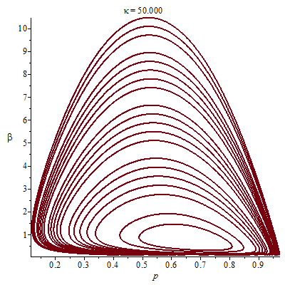
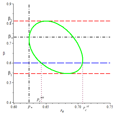
Figure 1: The left frame shows typical curves determined by equation $\kappa_{c}(p_{e},\beta,\delta)=\kappa$ on the $(p_{e},\beta)$ plane for $\kappa$ in the range from $15.12$ to $50.0$ and $\delta=(1,1,0,0)$. The area bounded by a curve increases with $\kappa$. The right frame corresponds to $\delta=(1,1,0,0)$ and $\kappa=13.56$. The other numerical values are: $p_{*}\approx 0.624$; $p_{c}^{un}\approx 0.642$, $p^{st}_{c}\approx 0.707$, $\beta_{1}\approx 0.546$, $\beta_{2}\approx 0.812$

Fig. 1 shows that the oscillatory instability of homogeneous equilibria occurs in response to growth of the predators density, $p_{e}$, provided that their motility is great enough; that is, $\kappa>\kappa_{*}(\delta)$. It follows from the results of [5, 6] that this oscillatory instability is accompanied by Poincare-Andronov-Hopf bifurcation manifested by excitation of waves, and, moreover, the wave dynamics turns out to be more advantageous than equilibrium in the sense that predators can consume more, while leaving greater stock of the prey. The value of $\kappa_{*}(\delta)>0$ is the threshold for the predators motility, $\kappa$. If $\kappa<\kappa_{*}(\delta)$ then neither the oscillatory instability of the homogeneous equilibrium nor the accompanying bifurcation are possible, whatever values of the predator density and the disturbances wavelengths are specified. Thus, the weakening of the predators motility leads to the absolute stabilization of the homogeneous equilibria and does not allow the community to adapt itself to the resource deficiency.

The Poincare-Andronov-Hopf bifurcation has been studied for more general classes of the PKS type systems in [7, 10, 11].

3 Fluctuating environment

In what follows, let’s consider every function of variables $(\xi,\tau)$ as a function defined on 2-torus $\mathbb{T}^{2}$. Define

$$\langle g\rangle=\frac{1}{4\pi}\int\limits_{0}^{2\pi}\int\limits_{0}^{2\pi}g(x,t,\xi,\eta)\,d\xi d\eta.$$ (3.1)

Let the external signal in Eq. (1.1) be a short wave, i.e.

$$f=f(x,t,\xi,\tau),\ \xi=\omega x,\ \tau=\omega t,\ \omega\gg 1$$ (3.2)

and let the diffusion rates in Eq. (1.1-1.2) be of the same order as the wave length, namely:

$$\delta_{u}=\nu_{1}\omega^{-1},\ \delta_{p}=\nu_{2}\omega^{-1},\ \nu_{1}>0,\ \nu_{2}>0.$$ (3.3)

With these assumptions, asymptotic of system (1.1)-(1.3) takes the following form

$$q(x,t)=\bar{q}(x,t)+O({\omega}^{-1}),\ \omega\to+\infty;$$ (3.4)

$$u(x,t)=\bar{u}(x,t)+\widetilde{u}_{0}(x,t,\tau,\xi)+O({\omega}^{-1}),\ \omega\to+\infty;$$ (3.5)

$$p(x,t)=\bar{p}(x,t)P(x,t,\tau,\xi)+O({\omega}^{-1}),\ \omega\to+\infty$$ (3.6)

$$\partial_{\tau}\widetilde{u}_{0}=\partial_{\xi}(f+\nu_{1}\partial_{\xi}\widetilde{u}_{0});\ \langle\widetilde{u}_{0}\rangle=0,$$ (3.7)

$$\partial_{\tau}P=\partial_{\xi}(\nu_{2}\partial_{\xi}P-P(\bar{u}+\widetilde{u}_{0})),\ \langle P\rangle=1;$$ (3.8)

$$\partial_{t}\bar{u}=\partial_{x}(\kappa\bar{q}+\sigma\bar{f})-\nu\bar{u};\ \bar{f}=\langle f\rangle$$ (3.9)

$$\partial_{t}\bar{p}+\partial_{x}(\bar{p}(\bar{u}+\langle\widetilde{u}_{0}P\rangle))=0;$$ (3.10)

$$\bar{q}_{t}=\bar{q}(1-\bar{p}-\bar{q})+\delta_{q}\partial^{2}_{x}\bar{q}.$$ (3.11)

Note that $\bar{u}=\langle u\rangle+O({\omega}^{-1}),\quad\bar{p}=\langle p\rangle+O({\omega}^{-1}),\quad\bar{q}=\langle q\rangle+O({\omega}^{-1}),\quad\omega\to+\infty.$

Eq. (3.10) governing the predators transport describes, in particular, a drift the velocity of which is $\langle\widetilde{u}_{0}P\rangle$. This drift is the only remembrance of the short-wavelength signal. The drift velocity is uniquely determined by $\bar{u}$ provided $f$ is specified. Therefore, Eqs.  (3.9), (3.10) and (3.11) form a closed system relative to unknowns $\bar{p},\bar{q},\bar{u}$. This is what we call as the homogenized system.

The details of derivation are placed in Appendix II.

4 Stabilization of quasi-equilibria

In what follows, we assume that

$$f={f}(\xi,\tau).$$ (4.1)

Under this assumption, Eqs. (3.7)-(3.8) imply that $\widetilde{u}_{0}$ is independent of $(x,t)$, and $P$ is independent of $(x,t)$ provided $\bar{u}=0$. Hence the homogenized system has a family of homogeneous equilibria

$$\bar{p}\equiv p_{e},\ \bar{q}\equiv q_{e},\ \bar{u}=0,\ p_{e}=\operatorname{const}>0,q_{e}=\operatorname{const}>0,\ p_{e}+q_{e}=1.$$ (4.2)

Formulae (3.4)–(3.6) together with Eqs. (3.7)-(3.8) identify every equilibrium (4.2) with a short-wavelength solution of the original system which we call quasi-equilibrium. In the quasi-equilibria, the predators velocity vanishes on average while the averaged densities of both species are constant (at least, in the leading approximation). In the considerations below the quasi-equilibria of the original system and homogeneous equilibria of the homogenized system are not actually distinguishable, and we shall use the same name for both.

Let us examine the linear stability of quasi-equilibria. Let $f=f(\xi,\tau)$ be given and $\widetilde{u}_{0}=\widetilde{u}_{0}(\xi,\tau)$ be determined by Eq. (3.7). Define the mapping $\mathbb{R}\to\mathbb{R}$ as follows

$$\eta\mapsto\langle\widetilde{u}_{0}P\rangle$$ (4.3)

where $P=P(\xi,\tau)$ is the solution to problem

$$\partial_{\tau}P=\partial_{\xi}(\nu_{2}\partial_{\xi}P-P(\eta+\widetilde{u}_{0})),\ \langle P\rangle=1.$$ (4.4)

Let $\mathcal{V}^{\prime}({f})$ denote the differential of mapping (4.3)-(4.4) evaluated at the origin. The system governing the evolution of a small perturbation of a given quasi-equilibrium takes the form

$$\partial_{t}\bar{u}+\nu\bar{u}-\kappa\partial_{x}\bar{q}=0;$$ (4.5)

$$\partial_{t}\bar{p}+{p}_{e}(1+\mathcal{V}^{\prime}({f}))\partial_{x}\bar{u}=0;$$ (4.6)

$$\partial_{t}\bar{q}+{q}_{e}(\bar{p}+\bar{q})-\delta_{q}\partial^{2}_{x}\bar{q}=0;$$ (4.7)

Note that factor $1+\mathcal{V}^{\prime}({f})$ can be treated as the effective motility coefficient.

Re-scaling $\bar{u}$, we transform system (4.5)-(4.7) into the form (2.2)-(2.4) with $\delta_{p}=\delta_{u}=0$, and $\kappa$ changed by $\bar{\kappa}=(1+\mathcal{V}^{\prime}({f}))\kappa$. Therefore, the effect of the short-wavelength external signal on the stability of quasi-equilibria manifests itself in altering the prey-taxis intensity or, equivalently, the predators motility in accordance with rule $\kappa\mapsto(1+\mathcal{V}^{\prime}({f}))\kappa$.

Note that restrictions (2.6) on the problem parameters imposed in Sec. 2 allows $\delta_{p}$ and $\delta_{u}$ to be zero simultaneously. Therefore all the statements about the stability of equilibria of the homogeneous version of system (1.1)-(1.3), made in Sec. 2, are also true regarding the stability of the quasi-equilibria, provided that the predators motility, $\kappa$, is replaced by its effective counterpart $\bar{\kappa}=(1+\mathcal{V}^{\prime}({f}))\kappa$. In particular, the inequality

$$1+\mathcal{V}^{\prime}({f})<{\kappa}^{-1}{\kappa_{*}|_{\delta_{p}=\delta_{u}=0}}$$ (4.8)

implies absolute stabilization of quasi-equilibria in the sense that there is no instability irrespective of what equilibrium and what the perturbation wave number are considered (here $\kappa_{*}$ is exactly the threshold motility of the predators introduced in Sec. 2).

The righthand side in inequality (4.8) does not depend on the external signal while the lefthand side evidently does depend and it is interesting to learn to what extent; in particular, whether or not a short-wavelength external signal is capable of the absolute stabilizing the equilibria which are unstable provided that the signal is off. More formally, the question is whether or not one can get inequality (4.8) by manipulating function $f$. Let’s show that the answer to this question is affirmative.

Let us denote as $\langle g\rangle^{\xi}$ the average value of some function $g=g(x,t,\xi,\tau)$ with respect to variable $\xi$; that is,

$$\langle g\rangle^{\xi}=\frac{1}{2\pi}\int\limits_{0}^{2\pi}g(x,t,\xi,\tau)\,d\xi$$ (4.9)

Let the external signal be independent of $\tau$:

$${f}={f}(\xi),\ \langle{f}\rangle=0.$$ (4.10)

Under condition (4.10), evaluation of $\tilde{u}_{0}$ reduces to the solving of equations

$$\partial_{\xi}(\sigma f+\nu_{1}\partial_{\xi}\widetilde{u}_{0})=0,\ \langle u_{0}\rangle^{\xi}=0.$$ (4.11)

Then evaluation of $P$ reduces to the solving of equations

$$\partial_{\xi}(\nu_{2}\partial_{\xi}P-P(\bar{u}+\widetilde{u}_{0}))=0,\ \langle P\rangle^{\xi}=1,$$ (4.12)

Consequently,

$$\mathcal{V}^{\prime}(f)=\langle\widetilde{u}_{0}P_{1}\rangle^{\xi}$$ (4.13)

where $P_{1}$ is determined by equations

$$\partial_{\xi}(\nu_{2}\partial_{\xi}P_{1}-P_{0}-\widetilde{u}_{0}P_{1})=0,\ \langle P_{1}\rangle^{\xi}=0,$$ (4.14)

$$\partial_{\xi}(\nu_{2}\partial_{\xi}P_{0}-\widetilde{u}_{0}P_{0})=0,\ \langle P_{0}\rangle^{\xi}=1.$$ (4.15)

Here we are interested only in those solutions to equations (4.11), (4.12), (4.14) and (4.15) which are $2\pi-$periodic in variable $\xi$.

Straightforward calculations, taking into account the periodicity, yield the following results

$$P_{0}=A_{0}\mathrm{e}^{v},\quad A_{0}=\frac{1}{\langle\mathrm{e}^{v}{\rangle^{\xi}}};$$ (4.16)

$$P_{1}=\mathrm{e}^{v}(A_{1}+\frac{\partial_{\xi}^{-1}(A_{0}-C_{1}\mathrm{e}^{-v})}{\nu_{2}}),\ A_{1}=\frac{A_{0}\langle\mathrm{e}^{v}\partial_{\xi}^{-1}(C_{1}\mathrm{e}^{-v}-A_{0}){\rangle^{\xi}}}{\nu_{2}},\ C_{1}=\frac{1}{\langle\mathrm{e}^{-v}{\rangle^{\xi}}\langle\mathrm{e}^{v}{\rangle^{\xi}}};$$ (4.17)

$$v=(\nu_{2}\partial_{\xi})^{-1}\tilde{u}_{0},$$ (4.18)

where transformation $\partial_{\xi}^{-1}$ acts on $2\pi$-periodic (in $\xi$) functions vanishing on average as the right inverse to $\partial_{\xi}$, i.e.

$$\partial_{\xi}\partial_{\xi}^{-1}w=w,\ \langle\partial_{\xi}^{-1}w\rangle^{\xi}=0$$

for any function $w$ such that it is $2\pi$-periodic in $\xi$ and $\langle w\rangle^{\xi}=0$. Consequently,

$$\mathcal{V}^{\prime}({f})=\nu_{2}\langle(A_{1}+\nu_{2}^{-1}\partial_{\xi}^{-1}(A_{0}-C_{1}\mathrm{e}^{-v}))\mathrm{e}^{v}\partial_{\xi}v{\rangle^{\xi}}=-\langle\mathrm{e}^{v}(A_{0}-C_{1}\mathrm{e}^{-v}){\rangle^{\xi}}=C_{1}-1=\frac{1}{\langle\mathrm{e}^{-v}{\rangle^{\xi}}\langle\mathrm{e}^{v}{\rangle^{\xi}}}-1.$$

Finally, the solving of problem (4.11) yields $\widetilde{u}_{0}=-(\nu_{1}\partial_{\xi})^{-1}{f}$, and then we get

$$v=(\nu_{2}\partial_{\xi})^{-1}\widetilde{u}_{0}=-(\nu_{2}\partial_{\xi})^{-1}(\nu_{1}\partial_{\xi})^{-1}{f}.$$

In what follows we change $f$ by $-f$. This does not lead to any mistakes since functional $\mathcal{V}^{\prime}({f})$ is even with respect to $f$. Thus the effective motility $\bar{\kappa}=(1+\mathcal{V}^{\prime}({f}))\kappa$ takes almost explicit form; namely

$$\bar{\kappa}=\frac{\kappa}{\langle\mathrm{e}^{-v}{\rangle^{\xi}}\langle\mathrm{e}^{v}{\rangle^{\xi}}},\quad v=(\nu_{1}\nu_{2})^{-1}\partial_{\xi}^{-2}{f}.$$ (4.19)

Substituting this into inequality (4.8) yields a more explicit form of the criterion for absolute stabilization:

$$\frac{1}{\langle\mathrm{e}^{-v}{\rangle^{\xi}}\langle\mathrm{e}^{v}{\rangle^{\xi}}}<\kappa^{-1}\kappa_{*}|_{\delta_{p}=\delta_{u}=0},$$ (4.20)

Example 1

Let $f=A\sin\xi$, $A=\operatorname{const}>0$. Then $v=-A(\nu_{1}\nu_{2})^{-1}\sin\xi$, and

$$\kappa\bar{\kappa}^{-1}=\langle\mathrm{e}^{-v}{\rangle^{\xi}}\langle\mathrm{e}^{v}{\rangle^{\xi}}=I^{2}_{0}(a),\ a=\frac{A}{\nu_{1}\nu_{2}}$$

where $I_{0}$ is the modified Bessel function of first kind. Consequently, the criterion for absolute stabilization (4.20) takes the following form

$$I^{-2}_{0}(a)<{\kappa}^{-1}\kappa_{*}|_{\delta_{p}=\delta_{u}=0},\ a=\frac{A}{\nu_{1}\nu_{2}}$$ (4.21)

The left hand side in this inequality decreases exponentially when parameter $a$ grows up. This parameter represents a characteristic amplitude of the external signal. Hence, the increase in the level of the external signal leads to absolute stabilization of the relative equilibria and this effect is rather powerful in the sense that the threshold of the absolute stabilization is attained exponentially fast.

Remark 1. In fact, the exponential decrease in effective motility of the predators in response to the increase in the level of external signal is a generic property of the system. This can be seen by estimating expression (4.19) using the Laplace method for $f=Af_{0}$, where $A\to\infty$ while choice of $f_{0}$ is rather wide. Therefore, the increase in the amplitude of short-wavelength external signal typically stabilizes the relative equilibria as is shown in Example 1.
Remark 2. The stabilization described above occurs irrespective of whether the external signal is attractive or repellent for the predators.

5 Conclusions

Thus the short-wavelength signal applied to PKS-type equations is capable of reducing the cross-diffusive transport on average drastically. Typically, the decrease in cross-diffusive motility in response to the increase in the signal level is exponential, and such the loss of motility exerts very powerful stabilizing effect on the primitive quasi-equilibria. An interesting question is to what extent the shape of the external signal is able to enhance or weaken the stabilizing effect of it. This question leads to an optimization problem for the effective motility defined in (4.19) subject to restriction $\langle f^{2}\rangle=1.$

Finally, we would like to relate the results described above to general phenomena which are often observed upon the application of the averaging and homogenization techniques. First, the additional cross-diffusive flux in Eq. (3.10) definitely resembles Stokes’s drift which typically arises upon the averaging of the advection of some matter over small-scale oscillations of the advective velocity [19]. Second, the short-wave stabilizing of quasi-equilibria resembles similar effects of high-frequency vibrations on the pendulum dynamics or on the stratified fluid dynamics [17, 18].

Acknowledgments

Andrey Morgulis acknowledges the support from Southern Federal University (SFedU)

6 Appendix I. Eigenmodes of the equilibria

Let us choose an equilibrium out of family (2.1) by specifying a value of the family parameter, $p_{e}$. Eigenvalues for the eigenmodes (2.5) having a specific wavenumber $\alpha$ are solutions to the following algebraic equation

$$\lambda^{3}+(D_{1}+D_{2}+D_{3})\lambda^{2}+(D_{2}D_{3}+D_{1}D_{3}+D_{1}D_{2})\lambda+D_{1}D_{2}D_{3}+\beta\kappa p_{e}q_{e}=0,$$ (6.1)

$$D_{1}=\nu+\beta\delta_{u};\ D_{2}=\beta\delta_{p};\ D_{3}=q_{e}+\beta\delta_{q};\ \beta=\alpha^{2}.$$

In view of restrictions (2.6), all the coefficients of the polynomial on the left hand side of Eq. (6.1) are strictly positive. Consequently, this polynomial has neither positive nor zero roots. Hence, no unstable or neutral eigenmode corresponds to a real eigenvalue.

It follows from the Routh-Hurwitz theorem that the necessary and sufficient condition for all roots of polynomial (6.1) to be in the open left half-plane of the complex plane is

$$(D_{1}+D_{2}+D_{3})(D_{2}D_{3}+D_{1}D_{3}+D_{1}D_{2})>D_{1}D_{2}D_{3}+\beta\kappa p_{e}q_{e}.$$

This inequality admits a more compact form, namely:

$$(D_{1}+D_{2})(D_{1}+D_{3})(D_{2}+D_{3})>\beta\kappa p_{e}q_{e}.$$

Hence the results of linear analysis described in Sec. 2 are valid provided that one defines the threshold magnitude for the predators motility as

$$\kappa_{c}=\frac{(D_{1}+D_{2})(D_{1}+D_{3})(D_{2}+D_{3})}{\beta p_{e}q_{e}}.$$ (6.2)

Indeed, the degree of polynomial (6.1) is 3. Consequently, $\kappa=\kappa_{c}$ is the necessary and sufficient condition for a root of polynomial (6.1) to lie on the imaginary axis (this root cannot be zero).

In the case $\delta_{u}=\delta_{p}=0$ which is of particular interest for the considerations of Sec. 4, the threshold takes much simpler form

$$\kappa_{c}|_{\delta_{p}=\delta_{u}=0}={\frac{{\nu}\,\left({\delta_{q}}\,\beta+{\nu}+q_{e}\right)\left({\delta_{q}}\,\beta+q_{e}\right)}{q_{e}\,p_{e}\beta}}.$$

7 Appendix II. Derivation of the asymptotic

Here we derive formally the asymptotic approximation described in Sec. 3.

On introducing the fast variables $\xi=\omega x$, $\tau=\omega t$ into the governing equations (1.1)-(1.3), they take the following form

$$\omega((\partial_{t}+\omega\partial_{\tau})u-(\partial_{x}+\omega\partial_{\xi})(\kappa q+\sigma f)+\nu u)=\nu_{1}(\partial_{x}+\omega\partial_{\xi})^{2}u;$$ (7.1)

$$\omega((\partial_{t}+\omega\partial_{\tau})p+(\partial_{x}+\omega\partial_{\xi})(up))=\nu_{2}(\partial_{x}+\omega\partial_{\xi})^{2}p;$$ (7.2)

$$(\partial_{t}+\omega\partial_{\tau})q-q(1-p-q)=\delta_{q}(\partial_{x}+\omega\partial_{\xi})^{2}q.$$ (7.3)

We look for an asymptotic expansion of the solution to system (7.1)-(7.3) in the form

$$(u,p,q)=\sum_{k\geqslant 0}\omega^{-k}(u_{k},p_{k},q_{k})(x,t,\xi,\tau),\omega\to\infty.$$ (7.4)

where all coefficients are required to be $2\pi-$periodic in $\xi$ and $\tau$. Substitution of (7.4) into system (7.1)-(7.3) and collecting terms of equal order in $\omega$ yields a sequence of equations which will be solved step by step.

Terms of order $\omega^{2}$ in Eq. (7.3) lead to the equation

$$\partial_{\xi\xi}q_{0}=0$$ (7.5)

that obviously has no periodic solutions except for solutions independent of $\xi$. Thus

$$q_{0}={q}_{0}(x,t,\tau).$$ (7.6)

where function ${q}_{0}$ is to be determined at the subsequent steps. In view of (7.6), the collecting of terms of order $\omega^{2}$ in Eqs. (7.1-7.2) leads to the equations

$$(\partial_{\tau}-\nu_{1}\partial_{\xi\xi})u_{0}=\sigma\partial_{\xi}f;$$ (7.7)

$$(\partial_{\tau}-\nu_{2}\partial_{\xi\xi})p_{0}+\partial_{\xi}(u_{0}p_{0})=0;$$ (7.8)

$$(u_{0},p_{0})=(u_{0},p_{0})(x,t,\xi,\tau),\ (\xi,\tau)\in\mathbb{T}^{2}.$$

Note that equation (7.7) is exactly the first equation in problem (3.7). Equation (7.7) has only one periodic solution vanishing on average in the sense of definition (3.1). We denote this solution as $\widetilde{u}_{0}$. Thus $u_{0}=\bar{u}+\widetilde{u}_{0}$, $\bar{u}=\langle u_{0}\rangle$, and we have justified the leading term in the asymptotic approximation for $u$, given by (3.5), (3.7).

We need the following
Lemma. Let $w=w(\xi,\tau)$ be a smooth $2\pi$-periodic (in both $\xi$ and $\tau$) function. Consider equation

$$\partial_{\tau}Q+\partial_{\xi}(wQ-{\epsilon}\partial_{\xi}Q)=0\ \text{on}\ \mathbb{T}^{2};\ {\epsilon}=\operatorname{const}>0.$$ (7.9)

Then there exists a unique $2\pi$-periodic (in $\xi$ and $\tau$) solution to Eq. (7.9) satisfying the additional condition

$$\langle Q\rangle=1.$$ (7.10)

Proof of this statement will be given in the end of this Appendix.

We continue constructing the asymptotic expansion. Equation (7.8) coincides with (7.9) up to the replacing ${\epsilon}$ by $\nu_{2}$ and $w$ by $\bar{u}+\widetilde{u}_{0}$, so that we can apply the above lemma, which yields

$$p_{0}=\bar{p}(x,t)P(x,t,\xi,\tau),$$ (7.11)

where $P$ is uniquely determined by (3.8). Hence we have justified the the leading term in the asymptotic approximation determined by (3.6) for unknown $p$.

Now let us consider the terms of order $\omega$. From Eq. (7.3), with the help of (7.6), we get

$$\delta_{q}\partial_{\xi\xi}q_{1}=\partial_{\tau}q_{0},$$ (7.12)

where $q_{0}$ does not depend on $\xi$. Hence, this equation has a periodic solution if and only if $q_{0}$ does not depend on $\tau$. Thus $q_{0}=\bar{q}(x,t)$ and we arrive at the leading term in the asymptotic approximation (3.4). Further, every solution to Eq. (7.12) has to have a form

$$q_{1}=q_{1}(x,t,\tau).$$ (7.13)

Functions $q_{1}$ and $\bar{q}$ are to be determined at subsequent steps of the procedure. Note that existence of a periodic solution to Eq. (7.12) justifies the error estimate (i.e. $O-$ term) in the asymptotic approximation (3.4).

Terms of order $\omega$ in Eq. (7.1)-(7.2), together with Eq. (7.13), lead to equations

$$(\partial_{\tau}u_{1}-\nu_{1}\partial_{\xi\xi})u_{1}=2\nu_{2}\partial_{x\xi}u_{0}+\partial_{x}(\kappa q_{0}+\sigma f)-\nu u_{0}-\partial_{t}u_{0},\quad(\xi,\tau)\in\mathbb{T}^{2};$$ (7.14)

$$\partial_{\tau}p_{1}+\partial_{\xi}(u_{0}p_{1})-\nu_{2}\partial_{\xi\xi}p_{1}=2\nu_{2}\partial_{x\xi}p_{0}-\partial_{t}p_{0}-\partial_{x}(u_{0}p_{0})-\partial_{\xi}(u_{1}p_{0}),\quad(\xi,\tau)\in\mathbb{T}^{2}.$$ (7.15)

On averaging Eqs. (7.14) and (7.15) and using (7.11), we obtain the homogenized system (3.9)-(3.11). Note that the resolving of the latter implies that Eqs. (7.14) and (7.15) have periodic solutions $u_{1}$ and $p_{1}$. This, in turn, justifies $O-$terms in the approximations (3.5) and (3.6)).

Now we get back to the above lemma. Before we start proving it in full generality, let us consider the particular case of $w=w(\xi)$. Then the periodic solution to Eq. (7.9) has to depend on a single variable $\xi$ and equation  (7.9) reduces to equation

$$\partial_{\xi}({\epsilon}\partial_{\xi}Q-wQ)=0.$$

Its general solution takes the form

$$Q=\exp\left({\epsilon}^{-1}\int w(\xi)d\xi\right)\int\limits\exp\left(-{\epsilon}^{-1}\int w(\xi)d\xi\right)d\xi$$

There is only one periodic solution among those given by this integral. To write it down explicitly, consider decomposition $w(\xi)=\langle w(\xi)\rangle+\widetilde{w}(\xi)$, and set

$$E(\xi)=\exp(({\epsilon}\partial_{\xi})^{-1}\widetilde{w}(\xi)).$$

Then

$$Q=AE(\xi)\int\limits_{0}^{\infty}\frac{\mathrm{e}^{-s}ds}{E(\xi+\frac{s}{\mu})},\ \text{where}\ \mu=\frac{\langle w(\xi)\rangle}{{\epsilon}}\neq 0,\ A=\operatorname{const}$$

and

$$Q=AE(\xi),\ \langle w(\xi)\rangle=0,\ A=\operatorname{const}.$$

Obviously, we can normalize the solution as required in (7.10) by suitable choice of $A$ in both cases but, for our purposes, we need to write down the periodic solution in a form that covers both cases. To do this, we consider the Fourier series

$$E(\xi)=\sum\limits_{k}\psi_{k}\mathrm{e}^{ik\xi},\quad E^{-1}(\xi)=\sum\limits_{k}\phi_{k}\mathrm{e}^{ik\xi}.$$

Then

$$Q=AE(\xi)\left(\phi_{0}+\mu\sum\limits_{k\neq 0}\frac{\phi_{k}\mathrm{e}^{ik\xi}}{\mu-ik}\right),\quad A^{-1}=\phi_{0}\psi_{0}+\mu\sum\limits_{k\neq 0}\frac{\phi_{k}\psi_{k}^{*}}{\mu-ik}$$

where $\psi_{k}^{*}$ are the complex-conjugate Fourier coefficients.

Let us pass to the general case. Let $\mathrm{H}$ be space of the Fourier series in $\xi,\tau$ with square-summable coefficients and let $\mathcal{L}:\mathrm{H}\to\mathrm{H}$ be operator defined by the left hand side of Eq. (7.9). We have to prove that

$$\dim\,\mathrm{Ker}\,\mathcal{L}=1,\ \langle w\rangle\neq 0\ \forall\ w\in\mathrm{Ker}\,\mathcal{L}\setminus\{0\}.$$ (7.16)

Let $\mathcal{L}^{*}$ denote the operator adjoint to $\mathcal{L}$. Define

$$\breve{\mathcal{L}}^{*}=\mathcal{{J}}\mathcal{L}^{*}\mathcal{{J}}$$

where $\mathcal{J}:\mathrm{H}\to\mathrm{H}$ is the action of inversion $(\xi,\tau)\mapsto(-\xi,-\tau)$. Then

$$\breve{\mathcal{L}}^{*}:\varphi\mapsto(\partial_{\tau}-{\epsilon}\partial_{\xi\xi})\varphi+w\partial_{\xi}\varphi.$$

Notice that PDE

$$(\partial_{\tau}-{\epsilon}\partial_{\xi\xi})\varphi+w\partial_{\xi}\varphi=0$$

obeys the strong maximum and minimum principles (see e.g. [23] or [24]). Hence,

$$\mathrm{Ker}\,\breve{\mathcal{L}}^{*}=\{\varphi\equiv\operatorname{const}\}=\mathrm{Ker}\,\mathcal{L}^{*}.$$

Applying unilateral strong maximum/minimum principles to PDE

$$(\partial_{\tau}-{\epsilon}\partial_{\xi\xi})\varphi+w\partial_{\xi}\varphi=1$$

shows that neither equation $\breve{\mathcal{L}}^{*}_{v}\breve{\psi}=1$ nor equation ${\mathcal{L}}^{*}_{v}\psi=1$ has a solution in $\mathrm{H}$. Consequently, the resolvent operator $(\mathcal{L}^{*}-\lambda\mathcal{I})^{-1}$, $\lambda\in\mathbb{C}$ has a simple pole at the origin. Moreover, since this resolvent is compact, the pair of operators $\mathcal{L}^{*}$ and $\mathcal{L}$ obeys the Fredholm theorems. Hence $\dim\,\mathrm{Ker}\,\mathcal{L}=1$. Furthermore, if $\langle w\rangle=0$ for some $w\in\mathrm{Ker}\,\mathcal{L}\setminus\{0\}$, this would imply the existence of solution to equation $\mathcal{L}^{*}\psi=\operatorname{const}\neq 0$ but this contradicts to what has been proved above. This completes the proof.
Remark. Let $\Pi^{*}$ denote spectral projector onto $\mathrm{Ker}\,\mathcal{L}^{*}$. Then the action of mapping (4.3)-(4.4) is identical to $\eta\mapsto\langle\Pi^{*}(\eta)\widetilde{u}_{0}\rangle$. Then the perturbation theory for linear operators implies that this mapping is differentiable and even analytic in a vicinity of origin, and that the derivative of this mapping denoted as $\mathcal{V}^{\prime}(f)$ can be evaluated in accordance with (4.13)-(4.14)-(4.15).

References

- [1] Ivanitskii GR, Medvinskii AB, Tsyganov, MA. (). From the dynamics of population autowaves generated by living cells to neuroinformatics. Physics-Uspekhi 1994; 37(10): 961.
- [2] Tsyganov MA, Brindley J, Holden AV., Biktashev VN. Quasisoliton interaction of pursuitevasion waves in a predator-prey system.Phys. Rev. Lett. 2003; 91(21): 218102-1-4.
- [3] Tsyganov MA, Brindley J, Holden AV, Biktashev VN. Soliton-like phenomena in one-dimensional cross-diffusion systems: a predator–prey pursuit and evasion example. Physica D: Nonlinear Phenomena 2004; 197(1-2): 18-33.
- [4] Tsyganov MA, Biktashev VN. Half-soliton interaction of population taxis waves in predator-prey systems with pursuit and evasion. Physical Review E 2004 70(3): 031901.
- [5] Govorukhin V, Morgulis A, Tyutyunov Y. Slow taxis in a predator-prey model. Doklady Mathematics 2000; 61(3): 420-422.
- [6] Arditi R, Tyutyunov Y, Morgulis A, Govorukhin V, Senina I. Directed movement of predators and the emergence of density-dependence in predator–prey models. Theoretical Population Biology 2001; 59(3): 207-221.
- [7] Pearce IG, Chaplain MAJ, · Schofield PG, Anderson ARA, Hubbard SF. Chemotaxis-induced spatio-temporal heterogeneity in multi-species host-parasitoid systems. J. Math. Biol. 2007; 55(3): 365–388.
- [8] Bellomo N,Bellouquid A, Tao Y, Winkler M. Toward a mathematical theory of Keller-Segel models of pattern formation in biological tissues. Math. Models Methods Appl. Sci. 2015; 25(09): 1663-1763.
- [9] Tello IJ , Wrzosek D. Predator–prey model with diffusion and indirect prey-taxis. Math. Models Methods Appl. Sci. 2016; 26(11): 2129-2162.
- [10] Tyutyunov Y, Titova L, Senina I. Prey-taxis destabilizes homogeneous stationary state in spatial Gause–Kolmogorov-type model for predator–prey system. Ecological Complexity 2017; 31: 170-180.
- [11] Wang Q, Yang J, Zhang L. Time-periodic and stable patterns of a two-competing-species Keller-Segel chemotaxis model: Effect of cellular growth. Discrete & Continuous Dynamical Systems - B. 2017; 22(9):3547-3574.
- [12] Li C, Wang X, Shao Y. Steady states of a predator–prey model with prey-taxis. Nonlinear Analysis: Theory, Methods and Applications. 2014; 97: 155-168.
- [13] Li U, Tao Y. Boundedness in a chemotaxis system with indirect signal production and generalized logistic source. Appl. Math. Letters 2018; 77: 108-113.
- [14] Black T. Boundedness in a Keller–Segel system with external signal production. Journ. of Math. Analysis Appl. 2017; 446(1): 436-455.
- [15] Yurk BP, Cobbold CA. Homogenization techniques for population dynamics in strongly heterogeneous landscapes. Journal of Biological Dynamics 2018; 12(1): 171-193.
- [16] Issa T, Shen W. Persistence, coexistence and extinction in two species chemotaxis models on bounded heterogeneous environments. 2018; arXiv preprint arXiv:1709.10040v4.
- [17] Yudovich V. The dynamics of vibrations in systems with constraints. Doklady Physics 1997; 42, 322-325.
- [18] Vladimirov V. On vibrodynamics of pendulum and submerged solid. Journ. of Math. Fluid Mech. 2005; 7 (S3): S397-S412.
- [19] Vladimirov V. Two-Timing Hypothesis, Distinguished Limits, Drifts, and Pseudo-Diffusion for Oscillating Flows. Studies in Appl. Math. 2017; 138(3): 269-293.
- [20] Allaire. G. A brief introduction to homogenization and miscellaneous applications. ESAIM: Proceedings. Vol. 37. EDP Sciences; 2012.
- [21] Allaire G. Homogenization and two-scale convergence. SIAM Journal on Math. Analysis 1992; 23(6): 1482-1518.
- [22] G. Allaire. Shape optimization by the homogenization method. Vol. 146. Springer Science & Business Media; 2012.
- [23] Nirenberg L. A strong maximum principle for parabolic equations. Comm. Pure Appl. Math. 1953; 6(2): 167-177.
- [24] Landis EM. Second order equations of elliptic and parabolic type. American Math. Soc.; 1997.