Unstable Equilibria and Invariant Manifolds in Quasi-Two-Dimensional Kolmogorov-like Flow

Abstract

Recent studies suggest that unstable, non-chaotic solutions of the Navier-Stokes equation may provide deep insights into fluid turbulence. In this article, we present a combined experimental and numerical study exploring the dynamical role of unstable equilibrium solutions and their invariant manifolds in a weakly turbulent, electromagnetically driven, shallow fluid layer. Identifying instants when turbulent evolution slows down, we compute 31 unstable equilibria of a realistic two-dimensional model of the flow. We establish the dynamical relevance of these unstable equilibria by showing that they are closely visited by the turbulent flow. We also establish the dynamical relevance of unstable manifolds by verifying that they are shadowed by turbulent trajectories departing from the neighborhoods of unstable equilibria over large distances in state space.

I Introduction

Understanding fluid turbulence has remained a long-standing problem in classical physics Hopf (1948); Landau and Lifshitz (1959); Arnold (2009). Recently, substantial progress was made using a theoretical framework that was originally developed Auerbach et al. (1987); Cvitanović (1988) for low-dimensional chaotic systems, such as the Lorentz system Lorenz (1963). This framework, which goes back to the work of Poincaré on celestial mechanics Poincaré (1993), uses a hierarchy of unstable temporally simple solutions (e.g., equilibria or periodic orbits) of the governing equations to provide both a dynamical and statistical description of a chaotic system. Computing such solutions of the Navier-Stokes equation – called Exact Coherent Structures (ECSs) – has become feasible only recently, following the development of novel numerical methods Saad and Schultz (1986); Kelley (1995).

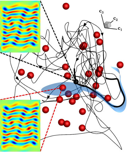
Figure 1: Low-dimensional projection of the state space (cf. Appendix A). Black curve is a trajectory describing the temporal evolution of a turbulent flow and red spheres represent different ECSs (equilibria in this particular case). Thick black line shows the portion of a turbulent trajectory shadowing (a portion of) the unstable manifold (blue surface) of an ECS. The flow (vorticity) fields in the physical space, corresponding to a particular point on the turbulent trajectory (black ball) and the nearest ECS, are shown on the left.

The dynamical role of ECSs in turbulence is best illustrated using a geometrical description Hopf (1948), where the flow field in physical space at any given instant is represented as a single point in a high-dimensional state space, as illustrated by figure 1. The evolution of the turbulent flow corresponds to a tortuous trajectory this point traces out in the state space Gibson et al. (2008). An infinite hierarchy of ECSs is conjectured to exist in regions of state space explored by turbulent trajectories. Near an ECS, the turbulent flow mimics both its spatial and temporal structure Gibson et al. (2008); Cvitanović and Gibson (2010); Suri et al. (2017), which is referred to as shadowing. However, being unstable, ECSs are visited only fleetingly Kerswell and Tutty (2007); Suri et al. (2017), and turbulent flow patterns never become identical to those corresponding to ECSs.

The geometry of state space around ECSs appears to be shaped by their invariant manifolds Wang et al. (2007); Gibson et al. (2008); Budanur et al. (2017a): turbulent trajectories approach an ECS following its stable manifold and depart following its unstable manifold Suri et al. (2017), at least when the spectrum associated with that ECS is not strongly nonnormal Schneider et al. (2017); Farano et al. (2018). Finally, heteroclinic (homoclinic) connections – which originate at one ECS and terminate at another (the same) ECS – are conjectured to guide turbulent trajectories between neighborhoods of ECSs Gibson et al. (2008); Halcrow et al. (2009); Riols et al. (2013). We will refer to both heteroclinic and homoclinic connections collectively as dynamical connections. In summary, turbulence can be viewed as a deterministic walk between neighborhoods of ECSs, guided by their invariant manifolds and dynamical connections.

Numerical simulations of three-dimensional (3D) wall-bounded shear flows, such as plane Couette Nagata (1997), channel Waleffe (2001), and pipe flows Faisst and Eckhardt (2003); Wedin and Kerswell (2004) at moderate Reynolds numbers $Re$ provide strong support for the dynamical relevance of ECSs. Equilibrium (EQ) and traveling wave (TW) solutions Nagata (1997); Waleffe (2001); Faisst and Eckhardt (2003); Wedin and Kerswell (2004) computed for minimal flow domains Hamilton et al. (1995) capture prominent spatial features (streamwise rolls and streaks) of near-wall coherent structures observed in experiments Kline et al. (1967). Certain periodic orbit (PO) and relative periodic orbit (RPO) solutions Kawahara and Kida (2001); Viswanath (2007) have been shown to describe self-sustained processes Hamilton et al. (1995); Waleffe (1997) responsible for destruction and reformation of near-wall coherent structures. Statistics of turbulent flows have also been found to agree well with those estimated using only a few ECSs Kawahara and Kida (2001); Viswanath (2007), suggesting statistical measures computed using a sufficiently large set of ECSs may indeed converge to those estimated using turbulent time series, providing a direct connection between dynamical and statistical description of turbulence.

While the framework has been developed primarily using numerical simulations, experimental evidence for the existence and dynamical relevance of ECSs in 3D shear flows remains scarce. Typically, in pipes and channels, the flow is measured using stereoscopic particle image velocimetry (PIV) within a planar cross section normal to the direction of mean flow. Taylor’s hypothesis is then invoked to reconstruct spatially resolved 3D velocity fields as flow structures are advected past the imaging plane. Using this technique, flow fields resembling TW solutions Faisst and Eckhardt (2003); Wedin and Kerswell (2004); Schneider et al. (2007a) were identified in pipe Hof et al. (2004); de Lozar et al. (2012); Dennis and Sogaro (2014) and channel Lemoult et al. (2014) flow experiments. Taylor’s hypothesis, however, breaks down where the mean flow is slow (e.g., near stationary walls), and no direct measurements of spatially and temporally resolved 3D velocity fields in experiments have been reported so far.

While numerous ECSs in various 3D shear flows have been computed, very few studies Kerswell and Tutty (2007); Budanur et al. (2017a) have tested how closely turbulent flows approach ECSs. Those studies, however, were limited to direct numerical simulations in short (less than 10 diameters long) pipes with periodic boundary conditions. Kerswell et al.aKerswell and Tutty (2007) have shown that turbulent flow at $Re=2400$ was found in the neighborhoods of TW solutions with $m-$fold ($m=2,3,4$) symmetry for about 10% of the time. An upper bound of about 20% for TWs at similar $Re$ was suggested by Schneider et al.aSchneider et al. (2007b). More recently, Budanur et al.aBudanur et al. (2017a) have tested how closely an RPO, the type of ECS conjectured to be dynamically more relevant than TWs, was shadowed by turbulent trajectories. No estimates are currently available for how closely turbulent trajectories in experiments approach ECSs.

The majority of the studies exploring invariant manifolds Gibson et al. (2008) focused on their role in direct laminar-turbulent transition Kerswell (2005); Eckhardt (2009) in 3D shear flows. Several TWs Itano and Toh (2001); Wang et al. (2007); Kerswell and Tutty (2007); Schneider et al. (2007a); Viswanath and Cvitanovic (2009); Budanur and Hof (2018) and POs Kawahara and Kida (2001); Toh and Itano (2003); Kawahara (2005); Viswanath (2007); Halcrow et al. (2009); Duguet et al. (2008) were found to lie on the laminar-turbulent boundary. The boundary itself can be constructed as the union of stable manifolds of these “edge states” and determines which nearby state space trajectories become turbulent and which relaminarize. However, the dynamical relevance of invariant manifolds in sustained 3D turbulence – either in simulation or experiment – is yet to be verified.

The dynamical relevance of ECSs (unstable equilibria) and their invariant manifolds, however, was recently established by Suri et al.aSuri et al. (2017) in the context of quasi-two-dimensional (Q2D) turbulence. Q2D flows, generated in shallow electrolyte layers driven by a horizontal electromagnetic force, are often studied as models of geophysical flows Van Heijst and Clercx (2009); Dolzhansky (2013). In experiments, spatially and temporally resolved velocity fields can be easily measured (at the electrolyte-air interface) using two-dimensional (2D) PIV, while the flow can be modeled using a strictly 2D equation Suri et al. (2014). This allowed Suri et al.ato compute 16 unstable equilibria of a Q2D Kolmogorov-like flow, directly using PIV data. Furthermore, it was shown that the evolution of turbulent trajectories, in both simulation and experiment, in the neighborhood of an ECS can be forecast by constructing its unstable manifold.

The goal of this article is to address some open questions regarding the dynamical role of unstable equilibria and their invariant manifolds, once again using the Q2D Kolmogorov-like flow as the test bed. Specifically, we show that turbulent flow in both the experiment and simulations comes quite close to almost all the unstable equilibria of the model that have been computed so far. Using a pair of representative equilibria we illustrate that, after turbulent trajectories enter the neighborhood of these ECSs they closely shadow the corresponding unstable manifolds for an extended period of time. The article is structured as follows: In sections II and III we present a brief overview of the experimental setup and numerical simulations, respectively. Our results are presented in Section IV and conclusions in Section V.

II Experimental Setup

The Kolmogorov flow used in classical investigations of hydrodynamic stability Meshalkin and Sinai (1961); Chandler and Kerswell (2013) refers to a strictly 2D flow driven by a sinusoidal forcing. Such a flow, however, is an idealization that is impossible to reproduce exactly in experiment. We will describe here an experimental setup that preserves, to the extent possible, its key features.

To create a nearly sinusoidal forcing, we arrange 14 NdFeB magnets (grade N42) to form an array of dimensions 15.24 cm$\times$($14\times 1.27$ cm)$\times$0.32 cm, as shown in figure 2(a). Adjacent magnets have opposite polarity, resulting in a nearly sinusoidal magnetic field ${\bf B}\approx B_{z}\hat{\bf z}$ with $B_{z}\approx e^{-\kappa z}\sin(\kappa y)$ at the center of the array. Here $\kappa=\pi/w$ and $w=1.27$ cm is the width of each magnet. The magnet array is placed on a horizontal aluminum plate and is padded with 0.32 cm thick aluminum bars to create a flat surface. A 50 $\mu$m-thick black contact paper is placed over this flat surface to provide uniform black background for better flow visualization. Acrylic bars and electrodes, running parallel to $y$ and $x$ axes respectively, are glued on top of contact paper to create a rectangular container of dimensions 17.8 cm$\times$22.9 cm with the magnet array at its center.

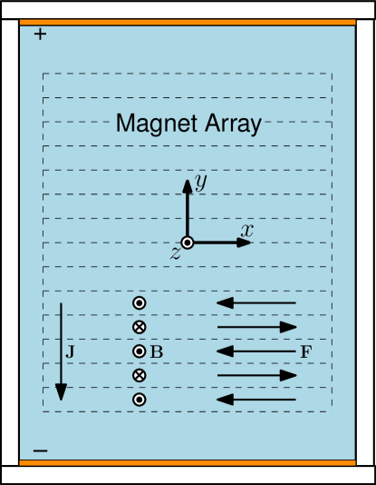
(a)

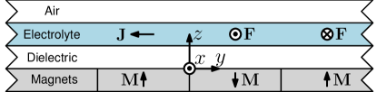
(b)

Figure 2: Schematic of the experimental apparatus. (a) Top view showing a magnet array with adjacent magnets (dashed lines) having magnetization in opposite directions (up/down/up/…). The array is placed over an aluminum plate and a container is constructed using acrylic end walls and copper electrode side walls. (b) Side view showing the cross section of the apparatus holding two immiscible fluid layers, a heavy dielectric and a lighter electrolyte. A direct current density ${\bf J}$ passing through the electrolyte interacts with the magnetic field ${\bf B}$ produced by the magnet array, exerting the Lorentz force ${\bf F}={\bf J}\times{\bf B}$. Spatiotemporally resolved 2D velocity fields are obtained using particle image velocimetry by imaging the tracer particles at the electrolyte-air interface with a camera (not shown) suspended above the container.

To create a nearly 2D flow, we use the two-immiscible-fluid layer configuration shown in figure 2(b). The bottom layer is a dielectric (perfluorooctane with density $\rho=1769$ kg/m³ and viscosity $\mu=1.3$ mPa$\cdot$s) and the top one is an electrolyte (1 M CuSO₄ with 40% glycerol by weight with density $\rho=1160$ kg/m³ and viscosity $\mu=5.7$ mPa$\cdot$s); each layer is 0.3 cm thick. Passing a uniform direct current density ${\bf J}=J\hat{\bf y}$ through the electrolyte generates a nearly sinusoidal Lorentz force ${\bf F}\approx{J}e^{-\kappa z}\sin(\kappa y){\,\bf\hat{x}}$ that drives the flow in both layers. The flow in the experiment is visualized by seeding the electrolyte-air interface with Glass Bubbles (K15) manufactured by 3M. Spatiotemporally resolved images of the entire lateral extent of the flow are recorded at 15 Hz using the DMK 31BU03 camera which has a 1024$\times$768 pixel CCD sensor. Velocity field ${\bf u}(x,y,t)$ at the electrolyte-air interface is calculated using the Prana PIV package Drew et al. (2013) employing the “Deform” multigrid PIV algorithm. The grid resolution of the resulting PIV measurements is about 120 $\times$ 160, or approximately 9 grid points per magnet width.

The dynamical regimes in the experiment are parametrized using the Reynolds number

$$Re=\frac{\bar{u}w}{\bar{\nu}}.$$ (1)

Here, $\bar{\nu}=3.26$ mm²/s is the depth-averaged kinematic viscosity of the two fluid layers Suri et al. (2014) and the characteristic velocity $\bar{u}$ is defined as the spatial root-mean-square average of ${\bf u}$ over the central $8w\times 8w$ region which is subsequently temporally averaged over the entire time-series.

III Theoretical Model

The evolution of the flow is modeled using a strictly 2D equation Suri et al. (2014)

$$\frac{\partial{\bf u}}{\partial t}+\beta{\bf u}\cdot\nabla{\bf u}=-\nabla p+\frac{1}{Re}\left(\nabla^{2}{\bf u}-\gamma{\bf u}\right)+\langle{{\bf F}_{\|}}\rangle_{z},$$ (2)

derived from first principles by averaging the 3D Navier-Stokes equation along the confined ($z$) direction. In the above equation $\langle{{\bf F}_{\|}}\rangle_{z}$ is the depth-averaged 2D force density while $p$ is the 2D kinematic pressure. The velocity field ${\bf u}=(u_{x},u_{y})$ in the 2D model is assumed to be incompressible ($\nabla\cdot{\bf u}=0$) which is a good approximation for $Re\leq 40$ Suri et al. (2014). In the experiment, the solid boundary at the bottom causes a vertical gradient in the magnitude of the horizontal velocity Satijn et al. (2001); Suri et al. (2014). Equation (2) describes the change in inertia of the fluid layers due to this gradient using prefactor $\beta<1$ to the nonlinear term and the term $-\gamma{\bf u}$ represents the associated viscous shear stresses in the bottom fluid layer. For the fluid layer configuration in our experiment, $\beta=0.83$ and $\gamma=3.22$ deviate significantly from values corresponding to a strictly 2D flow ($\beta=1$, $\gamma=0$). Lastly, equation (2) was non-dimensionalized by choosing $w$ (magnet width), $\bar{u}$, $w/\bar{u}$, and $\bar{u}^{2}$ as scale factors for length, velocity, time, and kinematic pressure $p$, respectively Tithof et al. (2017).

While the forcing profile near the center of the magnet array in experiment is sinusoidal, it is fairly complicated near the lateral boundaries. To accurately replicate such forcing profile, the effective forcing $\langle{{\bf F}_{\|}}\rangle_{z}$ in the 2D model is computed following a first principles approach. The magnet array in the experiment is modeled as a 3D lattice of uniformly magnetized dipoles, with dipoles in adjacent magnets pointing oppositely along ${\,\bf\hat{z}}$ and $-{\,\bf\hat{z}}$. The net magnetic field $B_{z}(x,y,z)$ produced by the dipole lattice is calculated and the 3D Lorentz force density ${\bf F}=JB_{z}{\,\bf\hat{x}}$ is depth-averaged to obtain the 2D force density Tithof et al. (2017).

In the case of uniform magnetization, the forcing profile is anti-symmetric under the coordinate transformation $\mathcal{R}_{xy}:(x,y)\rightarrow(-x,-y)$, i.e., $\mathcal{R}_{xy}\langle{{\bf F}_{\|}}\rangle_{z}=-\langle{{\bf F}_{\|}}\rangle_{z}$. $\mathcal{R}_{xy}$ is equivalent to rotation by $\pi$ about the $z-$axis passing through the center of the domain. Under $\mathcal{R}_{xy}$, the velocity field transforms as $\mathcal{R}_{xy}{\bf u}(x,y)\rightarrow-{\bf u}(-x,-y)$ which leads to equation (2) being equivariant under ${\mathcal{R}_{xy}}$. However, since the magnets used in the experiment are not uniformly magnetized and the bottom of the container is not perfectly horizontal, $\mathcal{R}_{xy}$ is weakly broken.

Direct numerical simulations based on the 2D equation (2) in its semi-discrete form LeVeque and Leveque (1992) are performed on a computational domain with lateral dimensions and no-slip velocity boundary conditions identical to those in the experiment. Velocity and pressure fields are spatially discretized on a 2D marker and cell (MAC) staggered grid of dimensions 280$\times$360. This corresponds to a resolution of 20 cells per magnet width with grid spacing $\delta x$=$\delta y$=0.05. Spatial derivatives in equation (2) are approximated using finite differences: the 2D Laplacian operator with a five-point central difference formula and the nonlinear term with a modified MAC formula Griebel et al. (1998). Temporal integration of equation (2) is performed using the P2 projection scheme to enforce incompressibility of the velocity field at each time step van Kan (1986); Armfield and Street (1999). Temporal update of linear terms uses the implicit Crank-Nicolson scheme and that of the nonlinear term uses the explicit Adams-Bashforth scheme Armfield and Street (1999). For all numerical data presented in this article, a time step $\delta t=1/110$ was used for temporal integration to ensure the CFL number ${\max\{{u_{x}},u_{y}\}\delta t/\delta x}\leq 0.5$. More details regarding numerical simulations can be found in Suri et al.aSuri et al. (2017) and Tithof et al.aTithof et al. (2017).

Since the lateral dimensions and boundary conditions in the experiment and the simulation are identical flow fields from the experiment, satisfying certain specific criteria described below, can be used to compute dynamically relevant ECSs. To facilitate this, the PIV measurements on the coarser $120\times 160$ grid are interpolated onto the finer $280\times 360$ simulation grid. The interpolated fields (${\bf u}_{*}^{exp}$) are then projected onto the divergence-free subspace employing Helmholtz-Hodge decomposition to obtain initial conditions ${\bf u}_{ic}^{exp}$ for the simulations Suri (2017). The maximum difference between ${\bf u}_{*}^{exp}$ and ${\bf u}_{ic}^{exp}$, computed as $\|{\bf u}_{ic}^{exp}-{\bf u}_{*}^{exp}\|/\|{\bf u}_{*}^{exp}\|$, across all initial conditions tested, was less than 0.025. This confirms the flow at the electrolyte-air interface is nearly incompressible at $Re=22.5$ (the Reynolds number considered herein).

IV Results

A quantitative study of the transition from laminar flow to turbulence in this system (using both experiment and numerical simulations) has recently been performed by Tithof et al.aTithof et al. (2017). As $Re$ increases, the flow undergoes a sequence of bifurcations and becomes weakly turbulent at $Re\approx 18$. In the remainder of this paper, we will focus on the dynamics and the role of ECSs at $Re=22.5$. To illustrate the characteristic dynamics and flow structures at this $Re$, we have included videos showing evolution of vorticity fields from experiment and simulation in supplemental material (videos 1 and 2). Temporal auto-correlation computation shows that the correlation time at this $Re$ is $\tau_{c}=27\pm 1$ s (cf. Appendix B). In the experiment, five separate $125\tau_{c}$-long (3600 s) runs were performed to search for signatures of invariant solutions. In addition, two $1000\tau_{c}$-long (28000 s) time-series were generated using numerical simulations. Velocity fields in both simulations and experiment were sampled at uniform intervals of $\Delta t=0.037\tau_{c}$ (1 s) for analyzing the dynamics.

A leading theory assumes that dynamically dominant ECSs underlying fluid turbulence correspond to temporally periodic solutions of the governing equations Cvitanović (1988); Kawahara and Kida (2001); Cvitanović (2013); Budanur et al. (2017b) and there is some evidence supporting this assumption. In particular, a previous numerical investigation Chandler and Kerswell (2013) of a 2D Kolmogorov flow (described by equation (2) with $\beta=1$ and $\gamma=0$) with periodic lateral boundary conditions found many tens of (relative) temporally periodic solutions visited by turbulent dynamics. Unlike the flow on a periodic domain, which has both continuous and discrete symmetries Chandler and Kerswell (2013); Tithof et al. (2017), the laterally bounded system here has only a discrete symmetry $\mathcal{R}_{xy}$ and so it has no relative solutions.

To identify signatures of time-periodic solutions guiding turbulent flow we perform recurrence analysis Eckmann et al. (1987) of the velocity field time series. A recurrence diagram, like the one shown in figure 3, represents a measure of how similar the flow field at an instant $t$ is compared with the flow field at a later instant $t+\tau$, quantified using the function

$$R(t,\tau)=\min_{g}\frac{\|{\bf u}(t)-g{\bf u}(t+\tau)\|}{\|{\bf u}(t)\|},$$ (3)

where $\tau>0$ and $g=\{1,\mathcal{R}_{xy}\}$ are the elements of the group of discrete symmetries of the flow. While turbulent flow fields are not invariant under $\mathcal{R}_{xy}$, a flow field ${\bf u}$ and its rotated version $\mathcal{R}_{xy}{\bf u}$ can recur in time with equal (comparable) likelihood in the simulation (experiment). Equation (3) accounts for this by identifying the closest recurrence among symmetry related copies.

Figure 3: A sample recurrence plot used to identify signatures of ECSs in weakly turbulent flow produced by our simulations. Low (high) values of $R(t,\tau)$ indicate that flow fields at two instants $t$ and $t+\tau$ are similar (different). The dashed line corresponds to the correlation time $\tau_{c}$.

In figure 3, a region representing a low value of $R(t,\tau)$ indicates a near-recurrence, which means that flow fields at instants $t$ and $t+\tau$ are similar. Deep local minima at $\tau>\tau_{c}$ (dark red islands) suggest that turbulent flow shadows a periodic orbit with temporal period $T\approx\tau$. To our surprise, both in simulation and experiment, very few ($\leq 10$) such near-recurrences were observed, suggesting time-periodic solutions are not the most dynamically important ECSs at $Re=22.5$.

Instead, the most prominent feature was the presence of dark red triangular regions with their base at $\tau=0$ and height comparable to $\tau_{c}$, like the ones at $t\approx-10,0,5,10$ in figure 3. Such features reflect significant slowing down of the evolution during which the flow becomes nearly time-independent. This is a signature of the turbulent trajectory visiting the neighborhood of an unstable equilibrium solution. This inference can be rationalized using the analogy of a rotating pendulum slowing down near its inverted position, which corresponds to an unstable equilibrium. The discussion hereafter will focus on identifying such unstable equilibria, their stability properties, and the dynamical role they play in shaping the evolution of nearby turbulent trajectories.

IV.1 Unstable Equilibrium Solutions

Unlike the inverted pendulum example, unstable equilibria of the governing equations describing the flow considered here are not known a priori. Hence, we hypothesize that the turbulent trajectory passes close an equilibrium when it is evolving sufficiently slowly. To identify such instants, we define the instantaneous state space speed $s(t)$ Suri et al. (2017); Neelavara et al. (2017) of the turbulent trajectory as the properly normalized rate of change in velocity fields

$$s(t)=\frac{\tau_{c}}{\|{\bf u}(t)\|}\left\|\frac{d{\bf u}}{dt}\right\|\approx\frac{\tau_{c}}{\Delta t}\frac{\left\|{\bf u}(t+\Delta t)-{\bf u}(t)\right\|}{\|{\bf u}(t)\|}.$$ (4)

In the above equation, $\Delta t=0.037\tau_{c}$ (1 s) is the interval between successive samples of velocity fields in both simulation and experiment.

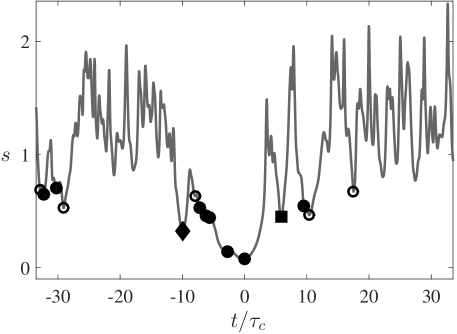
Figure 4: State space speed $s(t)$, with symbols indicating the deep local minima. Filled symbols designate a nearby unstable equilibrium was computed when the Newton-Krylov solver was initialized using the corresponding turbulent flow field. Different filled symbols represent convergence to distinct equilibria (cf. figure 5). Open circles indicate the solver failed to converge to an equilibrium.

Figure 4 shows the state space speed for the same segment of turbulent trajectory analyzed in figure 3. The position of the deep minima ($s\leq 0.7$), identified with symbols, closely corresponds to the location of the prominent red triangular regions in the recurrence plot. Note that the deepest minimum $\min_{t}s(t)=0.08$ is significantly lower than the temporal average of $s$, which is nearly unity. To determine whether these minima are associated with a nearby unstable equilibrium, we initialized a Newton-Krylov solver Kelley (2003); Mitchell (2013) using the turbulent flow fields which correspond to the respective minima. In several cases, labeled with filled symbols in figure 4, the solver identified a nearby unstable equilibrium ${\bf u}_{0}$. For some initial conditions ${\bf u}_{ic}$, however, the solver failed to converge to an equilibrium solution. Several different unstable equilibria were found this way, which we indicated using distinct symbols in figure 4. Here and below, $t=0$ denotes the global minimum of $s(t)$ within the temporal window shown.

The initial conditions, represented by contour plots of vorticity $\omega=(\nabla\times{\bf u})\cdot{\,\bf\hat{z}}$, are compared with the respective unstable equilibria of the 2D model in figure 5. The visual similarity of the corresponding flow states in the physical space is striking and unequivocally illustrates that turbulent trajectory passes very close to unstable equilibria, which is consistent with the dramatic slowdown in evolution. Notice that, since $\mathcal{R}_{xy}\omega(x,y)\rightarrow\omega(-x,-y)$, the equilibrium E01 is invariant under $\mathcal{R}_{xy}$, while E10 is not. In all, flow fields at 350 deep minima of $s(t)$ were tested for convergence in the simulation and 55 (about 15%) of these converged to 18 distinct unstable equilibria. While the temporal window in figure 4 shows a higher percentage of convergence, it was chosen since it includes the deepest minima across all the data.

(a)

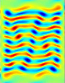
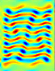
(a)

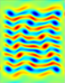
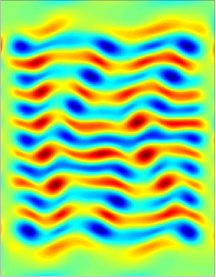
(b)

Figure 5: Equilibria (a) E01 and (b) E10 (see Table 1). The left column shows initial conditions from the numerical simulation corresponding to local minima (a) $t=0$ (black circle) and (b) $t=-10$ (black diamond) in figure 4. The right column shows the corresponding equilibria. The normalized distances from the initial conditions to E01 and E10 are $D_{0}^{ic}=0.20$ and $0.61$, respectively.

Failure of the Newton-Krylov solver to converge to an unstable equilibrium from a given initial condition does not necessarily indicate that there is no unstable equilibrium nearby, since convergence is only guaranteed for sufficiently close initial conditions. It is quite likely that a more robust solver, such as an adjoint-based one Farazmand (2016), might identify additional unstable equilibria. It is also worth noting that the success or failure of the Newton-Krylov method is correlated with the value of $s(t)$ at the local minimum (i.e., the success rate is the highest for the deepest minima), but the correlation is not perfect, as illustrated by figure 4. This is not surprising, given the highly anisotropic structure of chaotic sets, such as the one underlying turbulent dynamics of the Kolmogorov flow, in the state space.

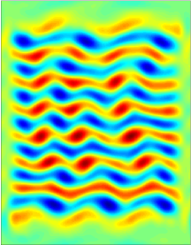
(a)

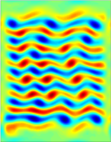
(b)

Figure 6: Equilibrium E20: (a) initial condition from the experiment and (b) the corresponding solution. The normalized difference between the two flow fields is $D_{0}^{ic}=0.33$. The colormap used here and below is the same as in figure 5.

Following a similar methodology, several equilibria of the 2D model were also computed by initializing the Newton-Krylov solver with processed PIV data from experiment. As an illustration, figure 6 shows the flow field corresponding to a minimum of $s(t)$ and the corresponding equilibrium. Due to the relatively short duration (125$\tau_{c}$) of each experimental run, a higher threshold $s\leq 1.1$ was chosen to identify a number of minima comparable to that in the simulations. From about 300 initial conditions from the five experimental runs, 24 (about 8%) converged to 19 distinct equilibria.

Sol	$\|{\bf u}_{0}\|$	IC	$\min\limits_{ic}D_{0}^{ic}$	$\min\limits_{t}D^{sim}_{0}(t)$	$\min\limits_{t}D^{exp}_{0}(t)$	$N_{{u}}$	$N_{KY}$	$\lambda_{1}$	$\sum\limits_{k=1}^{N_{u}}\lambda_{k}$
E01	254.7	S,E	0.14,0.69	0.13	0.57	2	4.53	0.0272	0.0517
E02	258.2	S	0.50	0.27	0.40	8	13.6	0.1508	0.2420
E03	258.4	S,E	0.24,0.39	0.19	0.35	7	13.0	0.1492	0.1922
E04	259.5	S	0.41	0.35	0.40	6	11.1	0.1422	0.2053
E05	261.1	E	0.82	0.72	0.67	7	14.4	0.1926	0.4916
E06	261.6	S	0.38	0.34	0.50	6	9.90	$0.0521+0.0458$	0.1257
E07	263.4	E	0.69	0.61	0.53	8	15.7	0.1222	0.3868
E08	264.1	S	0.50	0.49	0.47	3	6.81	$0.0344+0.0708i$	0.0828
E09	267.0	S	0.60	0.46	0.48	6	17.5	$0.1514+0.1097i$	0.6892
E10	267.3	S	0.61	0.47	0.50	5	13.3	$0.1074+0.0243i$	0.3991
E11	267.4	S,E	0.42,0.48	0.41	0.47	5	12.2	0.0896	0.2216
E12	267.6	S	0.70	0.44	0.49	3	10.7	$0.0775+0.0390i$	0.1726
E13	267.7	S	0.61	0.45	0.45	5	10.1	$0.0231+0.1900i$	0.0914
E14	267.9	S	0.42	0.39	0.50	6	14.0	$0.0922+0.0312i$	0.3493
E15	268.3	E	0.61	0.48	0.50	6	15.9	$0.1911+0.0737i$	0.5934
E16	268.7	E	0.63	0.53	0.37	5	10.9	$0.0749+0.0775i$	0.2482
E17	268.8	E	0.63	0.63	0.57	6	16.2	$0.1249+0.1935i$	0.4468
E18	269.2	S,E	0.49,0.54	0.49	0.46	6	16.9	0.1608	0.4230
E19	270.7	E	0.64	0.61	0.49	8	17.0	$0.1106+0.1261i$	0.4072
E20	272.4	S,E	0.53,0.33	0.41	0.33	4	15.3	$0.1014+0.1787i$	0.2977
E21	273.3	E	0.49	0.48	0.46	6	19.6	$0.1786+0.0852i$	0.5520
E22	274.0	E	0.71	0.54	0.56	9	20.3	0.2440	0.7611
E23	274.1	S	0.40	0.36	0.41	7	18.6	$0.1318+0.1681i$	0.3942
E24	275.7	E	0.61	0.56	0.49	7	16.0	0.1847	0.3497
E25	275.8	S,E	0.54,0.53	0.38	0.40	8	17.2	$0.1134+0.1611i$	0.4019
E26	276.1	S	0.33	0.33	0.49	3	8.99	$0.0284+0.1235i$	0.0752
E27	277.2	S	0.43	0.40	0.48	4	8.56	$0.0394+0.0896i$	0.1165
E28	278.6	E	0.70	0.50	0.49	6	17.7	$0.1037+0.0325i$	0.4475
E29	278.8	E	0.48	0.49	0.44	5	14.6	$0.1015+0.2180i$	0.3721
E30	279.8	E	0.60	0.46	0.49	7	17.9	0.2433	0.4565
E31	279.9	E	0.58	0.39	0.42	9	19.4	0.0723	0.3135

Table 1: Unstable equilibria (${\bf u}_{0}$) computed using initial conditions (IC) from simulation (S) and experiment (E), sorted by their $L2-$norm $\|{\bf u}_{0}\|$. $\min_{ic}D_{0}^{ic}$ is the distance from an equilibrium to the nearest initial condition (experimental or numerical) that converged to it under Newton’s iteration. $\min_{t}D_{0}^{sim}(t)$ ($\min_{t}D_{0}^{exp}(t)$) are the distances of the closest approach of turbulent trajectory in simulation (experiment) to an equilibrium. $N_{u}$ is the number of unstable eigenvalues and $N_{KY}$ is the local Kaplan-Yorke dimension. Eigenvalues are ordered by their real parts, with $\lambda_{1}$ being the most unstable one.

Among all of the equilibria calculated, six were found using both experimental and numerical initial conditions, resulting in a total of 31 distinct equilibria. Due to the equivariance of the governing equation under $\mathcal{R}_{xy}$, if ${\bf u}_{0}$ is an equilibrium which is not invariant under $\mathcal{R}_{xy}$, then its rotated copy $\mathcal{R}_{xy}{\bf u}_{0}\,(\neq{\bf u}_{0})$ is also an equilibrium. Consequently, distinct initial conditions may converge to either ${\bf u}_{0}$ or $\mathcal{R}_{xy}{\bf u}_{0}$. Hence, the converged equilibria were tested for presence of symmetry related copies to determine the total number of distinct ones. Table 1 lists all the distinct equilibria we computed, labeled in ascending order of their $L_{2}$-norm $\|{\bf u}_{0}\|$. Also listed are the data sets which contained the initial conditions that converged to a particular solution: simulation (S), experiment (E), or both (S,E).

The Newton-Krylov solver initialized using ${\bf u}_{ic}$ can, in principle, converge to an equilibrium ${\bf u}_{0}$ that lies far away from that initial condition. The degree of similarity between these two states can be quantified using the normalized distance

$$D_{0}^{ic}=\frac{\|{\bf u}_{ic}-{\bf u}_{0}\|}{\|{\bf u}_{0}\|}.$$ (5)

and is listed in Table 1 for each equilibrium. When several different initial conditions converged to an equilibrium, the smallest $D_{0}^{ic}$ was used. To relate the magnitude of $D_{0}^{ic}$ with the visual similarity between the flow fields ${\bf u}_{ic}$ and ${\bf u}_{0}$ in the physical space, we have included in the supplemental material the vorticity fields of all the equilibria and the nearest initial conditions. A quick comparison suggest that ${\bf u}_{ic}$ and ${\bf u}_{0}$ appear similar when $D_{0}\lesssim 0.60$. For example, the converged solution E10 and the corresponding initial condition shown in figure 5(b) bear a striking resemblance despite differing by $D_{0}^{ic}=0.61$.

To test how close the turbulent flows in experiments and simulations approach each equilibrium, we computed the minimal (normalized) distance

$$D_{0}(t)=\min_{g}\frac{\|{\bf u}(t)-g{\bf u}_{0}\|}{\|{\bf u}_{0}\|}.$$ (6)

Table 1 lists the minimal distances $\min_{t}D^{sim}_{0}(t)$ and $\min_{t}D^{exp}_{0}(t)$ from each equilibrium to turbulent trajectories in simulation and experiment, respectively. The data presented in Table 1 shows that, based on a threshold of 0.6, all but four (E05, E07, E17, and E19) equilibria were visited by the turbulent flow in both experiment and simulations, validating their dynamical relevance. Moreover, despite a shorter time series in the experiment, $\min_{t}D_{0}^{exp}(t)$ is not systematically higher than $\min_{t}D_{0}^{sim}(t)$ (except for E01,), confirming that equilibria of the 2D model are indeed dynamically relevant in the experiment. We note that only four equilibria computed – E01, E05, E06, and E26 – are invariant under $\mathcal{R}_{xy}$ and trajectories in the experiment, where $\mathcal{R}_{xy}$ is weakly broken, may not approach these solutions as closely as numerical trajectories might.

IV.2 Invariant Manifolds of Equilibria

The dynamical role of equilibria goes beyond causing slowdowns in the evolution of turbulent trajectories entering their neighborhoods. Their stable and unstable manifolds shape the state space geometry, guiding nearby turbulent trajectories, which follow the stable manifold of an equilibrium on approach and the unstable manifold on departure. The local orientation and the dimensionality of the stable and unstable manifolds are determined, respectively, by the stable and unstable eigenvectors of the corresponding equilibrium. As Table 1 shows, the number of unstable directions $N_{u}$ is small: it varies between 2 and 9 for all the equilibria we identified, which is a tiny fraction of the dimensionality of the full state space, $N_{f}\approx 2\times 10^{5}$.

On the contrary, the total number of stable directions, $N_{f}-N_{u}$, is very large, which appears to suggest a dramatic asymmetry between stable and unstable manifolds. However, only a tiny fraction of the degrees of freedom associated with the stable manifold play a role in sustained fluid turbulence, with dissipation constraining the dynamics to a relatively low-dimensional chaotic attractor Hopf (1948); Ruelle and Takens (1971); Brandstäter et al. (1983). The number of dynamically relevant degrees of freedom in the neighborhood of an equilibrium can be estimated by computing the local Kaplan-Yorke dimension Farmer et al. (1983)

$$N_{KY}=k_{0}+{\frac{1}{|\Re(\lambda_{k_{0}+1})|}}\sum\limits_{k=1}^{k_{0}}\Re(\lambda_{k}),$$ (7)

where the eigenvalues $\lambda_{k}$ are sorted by their real parts $\Re(\lambda_{k})$ in descending order and $k_{0}$ is the largest integer for which the sum on the right-hand-side of (7) is non-negative. For the equilibria considered here $N_{KY}(\approx 2N_{u})$ varies roughly between 4 and 20, suggesting that the number of dynamically relevant stable directions $N_{KY}-N_{u}$ is $O(10)$. To test if $N_{KY}$ corresponding to dynamically relevant ECSs is comparable to that of the attractor, we computed the Lyapunov spectrum of the chaotic attractor using continuous Gram-Schmidt orthogonalization Christiansen and Rugh (1997). Temporal average of the spectrum showed $N_{KY}\approx 15$, which is indeed comparable to $N_{KY}$ corresponding to the equilibria we computed.

Although the numbers of dynamically relevant stable and unstable directions in the neighborhood of the equilibria listed in Table 1 are comparable, in the remainder of this paper we will focus on unstable manifolds. They can be computed more easily using forward time integration and are also more useful in practice, e.g., allowing forecasting of the evolution of turbulent flows Suri et al. (2017). Two different examples, one with a pair of unstable eigenvalues with comparable magnitude and another characterized by a dominant real eigenvalue, will be used below to illustrate the dynamical role of the manifolds.

IV.2.1 Two-Dimensional Unstable Manifold

Equilibrium E01 shown in figure 5(a) has just two unstable eigenvectors ${\,\bf\hat{e}}_{1}$ and ${\,\bf\hat{e}}_{2}$, both with real eigenvalues $\lambda_{1}=0.0272$ and $\lambda_{2}=0.0245$. The perturbations corresponding to ${\,\bf\hat{e}}_{1}$ and ${\,\bf\hat{e}}_{2}$ in physical space are included in Appendix A. The 2D unstable manifold of E01 is locally tangent to the plane defined by ${\,\bf\hat{e}}_{1}$ and ${\,\bf\hat{e}}_{2}$, but deviates from this plane farther away due to nonlinearity. It was therefore computed using a dense set of 1440 trajectories ${\bf u}_{\theta}(t^{\prime})$ with initial conditions uniformly distributed around a circle ${\bf u}_{\theta}(0)={\bf u}_{0}+\epsilon\cos(\theta){\,\bf\hat{e}}_{1}+\epsilon\sin(\theta){\,\bf\hat{e}}_{2}$ with $\epsilon=10^{-4}\times\|{\bf u}_{0}\|$. The time $t^{\prime}$ and angle $\theta$ uniquely parametrize this 2D manifold.

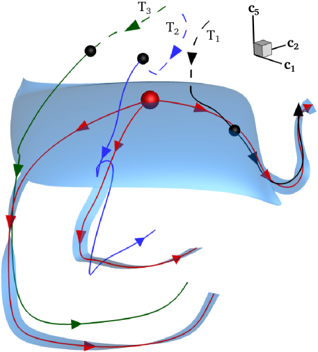
Figure 7: Turbulent trajectories ($\textrm{T}_{1}$, $\textrm{T}_{2}$, $\textrm{T}_{3}$) from numerical simulation shadowing the 2D unstable manifold (blue surface) of equilibrium E01 (red sphere). Black spheres on $\textrm{T}_{1}$, $\textrm{T}_{2}$, $\textrm{T}_{3}$ mark minima in $s(t)$. The portion of the unstable manifold shown was constructed using a one-parameter family of trajectories. Blue ribbons and red curves represent manifold extensions and reference manifold trajectories that $\textrm{T}_{1}$, $\textrm{T}_{2}$, and $\textrm{T}_{3}$ follow. The procedure used to construct this low-dimensional projection and the definition of basis vectors ${\bf c}_{i}$ are described in Appendix A.

A few of the manifold trajectories ${\bf u}_{\theta}(t^{\prime})$ along with a portion of the unstable manifold are shown in figure 7, which was constructed by projecting the high-dimensional state space onto an orthonormal basis spanned by the unstable eigenvectors ${\,\bf\hat{e}}_{1}$, ${\,\bf\hat{e}}_{2}$, and a stable eigenvector ${\,\bf\hat{e}}_{5}$ (cf. Appendix A). Note that all the trajectories lying in the manifold exhibit very little curvature near the equilibrium, which is a consequence of the two unstable eigenvalues being nearly equal. However, away from E01, the nonlinearity of the governing equation results in significant curvature of the manifold and nearby trajectories.

As we mentioned previously, sufficiently close passes to E01 were not observed in the experiment. In contrast, turbulent trajectories ${\bf u}(t)$ in the simulation were found to approach E01 very closely on numerous occasions. Three such trajectories with $\min_{t}D_{0}$ = 0.13 ($\textrm{T}_{1}$), 0.26 ($\textrm{T}_{2}$), and 0.26 ($\textrm{T}_{3}$) are shown in figure 7. The segments of these trajectories shown are approximately $10\tau_{c}$, $8\tau_{c}$, and $7\tau_{c}$-long, respectively. The trajectory $\textrm{T}_{1}$ corresponds to the deepest minimum of $s(t)$ as well as the closest approach to E01 across the entire time series (cf. figure 4).

Figure 7 shows that nearby turbulent trajectories indeed approach E01 along the stable manifold (in this projection along c₅) and subsequently depart following its unstable manifold. The segment of each turbulent trajectory as it approaches E01 is plotted using a dashed curve, while that following the unstable manifold is plotted using a solid curve. Notice that turbulent trajectories departing the neighborhood of E01 are guided by the unstable manifold even very far away from E01, where the linearization used to compute the eigenvalues and eigenvectors completely breaks down, as illustrated by the curvature of the manifold.

To make sure that the low-dimensional projection accurately reflects the dynamics in the full state space, we performed a quantitative analysis of the turbulent trajectories passing through the neighborhood of E01. We started by computing the instantaneous distance $D_{1}$ between a turbulent trajectory ${\bf u}(t)$ and each manifold trajectory ${\bf u}_{\theta}(t^{\prime})$:

$$D_{1}(t,\theta)=\min_{t^{\prime}}\frac{\|{\bf u}(t)-{\bf u}_{\theta}(t^{\prime})\|}{\|{\bf u}(t)\|}.$$ (8)

For a point ${\bf u}(t)$ on the turbulent trajectory, $D_{1}$ is the distance to the closest point – parametrized by $t^{\prime}$ – on a manifold trajectory ${\bf u}_{\theta}(t^{\prime})$. We then computed the instantaneous distance from the turbulent trajectory to the entire 2D unstable manifold parametrized by $\theta$ and $t^{\prime}$:

$$D_{2}(t)=\min_{\theta}D_{1}(t,\theta)=\min_{\theta,t^{\prime}}\frac{\|{\bf u}(t)-{\bf u}_{\theta}(t^{\prime})\|}{\|{\bf u}(t)\|}.$$ (9)

$D_{2}$ can be used to identify the manifold trajectory ${\bf u}_{\theta}$ which is the closest to the turbulent trajectory ${\bf u}(t)$ at a given instant.

Figure 8 shows the value of $\theta$ that corresponds to $D_{2}(t)$ for the three turbulent trajectories that appear in figure 7. In each case, $t=0$ corresponds to a minimum of $s(t)$, and only the temporal interval during which $\theta$ does not experience abrupt changes is plotted. We find that there is a fairly long time interval centered around $t=0$ over which $\theta\approx\theta_{c}=\theta|_{t=0}$ is essentially constant, i.e, each turbulent trajectory follows a specific reference trajectory ${\bf u}_{\theta_{c}}(t^{\prime})$ lying in the manifold. The reference trajectories in the unstable manifold corresponding to $\textrm{T}_{1}$, $\textrm{T}_{2}$, and $\textrm{T}_{3}$ are plotted in red in figure 7.

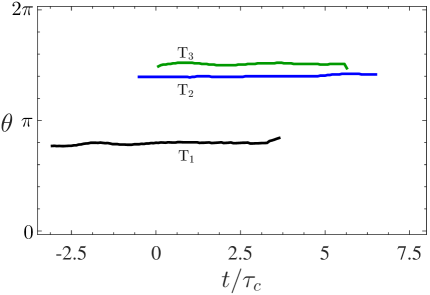
Figure 8: The angle $\theta$ for the manifold trajectory which is closest to the points ${\bf u}(t)$ on a nearby turbulent trajectory.

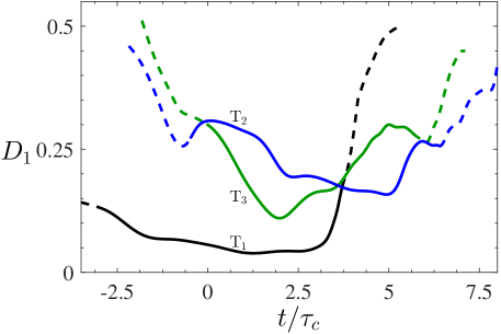
Figure 9: The distance between the turbulent trajectory ${\bf u}(t)$ and the corresponding manifold trajectory ${\bf u}_{\theta_{c}}(t^{\prime})$ (see text).

The distance between each turbulent trajectory and the corresponding manifold reference trajectory is given by $D_{1}(t,\theta_{c})$. In figure 9 we plot $D_{1}(t,\theta_{c})$ for each of the three turbulent trajectories shown in figure 7. Solid curves indicate the time intervals over which $\theta\approx\theta_{c}$ and so $D_{1}(t,\theta_{c})\approx D_{2}(t)$ is an accurate estimate of the distance from the turbulent trajectory to the entire unstable manifold. The relatively low values of the distance indicate that turbulent trajectories follow the corresponding manifold trajectories quite closely in the full state space for at least $3.5\tau_{c}$ following the instant at which $s(t)$ is a minimum.

Additional evidence for the dynamical role of the unstable manifold is provided in figure 10, which compares the flow field on ${\textrm{T}}_{1}$ – at a location which is far from E01 in the full state space – with the nearest point on the reference manifold trajectory. These states correspond to the ends of the respective trajectories in figure 7, where $D_{1}\approx 0.3$. The striking similarity between these flow fields once again confirms the hypothesis that turbulent flow is guided in state space by the unstable manifold (of E01 in this case) even when the flow has evolved substantially far away from the unstable equilibrium.

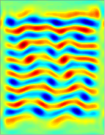
(a)

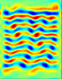
(b)

Figure 10: Flow fields for (a) the turbulent trajectory $\textrm{T}_{1}$ in figure 7 at $t/\tau_{c}=3.75$ and (b) the nearest point on the reference manifold trajectory.

As figure 9 shows, all three turbulent trajectories continue to approach the unstable manifold as they evolve farther away from the equilibrium. Indeed, the unstable manifold should be locally attracting for all initial conditions in the immediate neighborhood of the corresponding equilibrium. The unusual aspect here is that none of the three turbulent trajectories come particularly close to E01: the separations $D_{2}(0)\approx D_{1}(0)$ are between 0.1 and 0.3, which is outside the linear neighborhood of E01. Since the flow is chaotic, the unstable manifold becomes repelling far from the equilibrium. So even turbulent trajectories that approach the unstable manifold fairly closely eventually diverge away from it (cf. figure 9). This divergence imposes an inherent limit on the distance in state space over which turbulent trajectories are guided by any of the unstable manifolds.

In conclusion of this section, we comment on a dynamical aspect of the problem. The evidence we presented illustrates the geometrical role of the unstable manifold of E01 and particular manifold trajectories. However, one can ask whether the rate of evolution along the turbulent trajectory ${\bf u}(t)$ is the same as that for the corresponding manifold trajectory ${\bf u}_{\theta_{c}}(t^{\prime})$. Figure 11 shows the evolution of the “manifold time” $t^{\prime}$, which corresponds to points along ${\bf u}_{\theta_{c}}$ closest to ${\bf u}(t)$. Note that the origin for $t^{\prime}$ is arbitrary and was chosen to minimize the difference between $t$ and $t^{\prime}$. Although, for all three turbulent trajectories, the graphs of $t^{\prime}(t)$ cluster around the diagonal, which corresponds to identical rates of evolution for $t$ and $t^{\prime}$, there are notable deviations. For instance, we find a rather unexpected feature in the evolution of the turbulent trajectory $\textrm{T}_{2}$: $t^{\prime}$ decreases for $3\lesssim t/\tau_{c}\lesssim 4$. Indeed, during the corresponding time interval, this turbulent trajectory makes a small loop in figure 7. This odd behavior has to do with weakly stable degrees of freedom, which feature oscillatory dynamics.

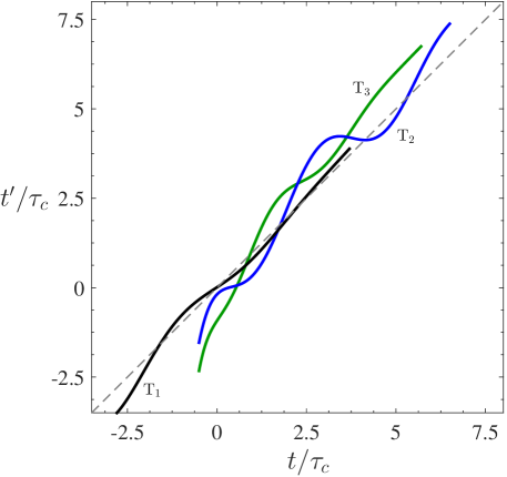
Figure 11: Comparison between the rates of evolution along manifold and turbulent trajectories.

IV.2.2 Seven-Dimensional Unstable Manifold

The analysis presented in the previous section suggests that turbulent evolution, following a deep minimum in $s(t)$, can be forecast for a few correlation times by constructing the unstable manifold of the nearby equilibrium. Such forecasting in both experiment and simulation for a close pass to E03 (cf. figure 12) was previously reported by Suri et al.aSuri et al. (2017). Here, we extend that study by providing quantitative estimates for the separation between the unstable manifold of E03 and nearby turbulent trajectories.

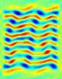
(a)

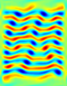
(b)

Figure 12: (a) A flow field from the experiment during a close pass to (b) equilibrium E03 which has a seven-dimensional unstable manifold.

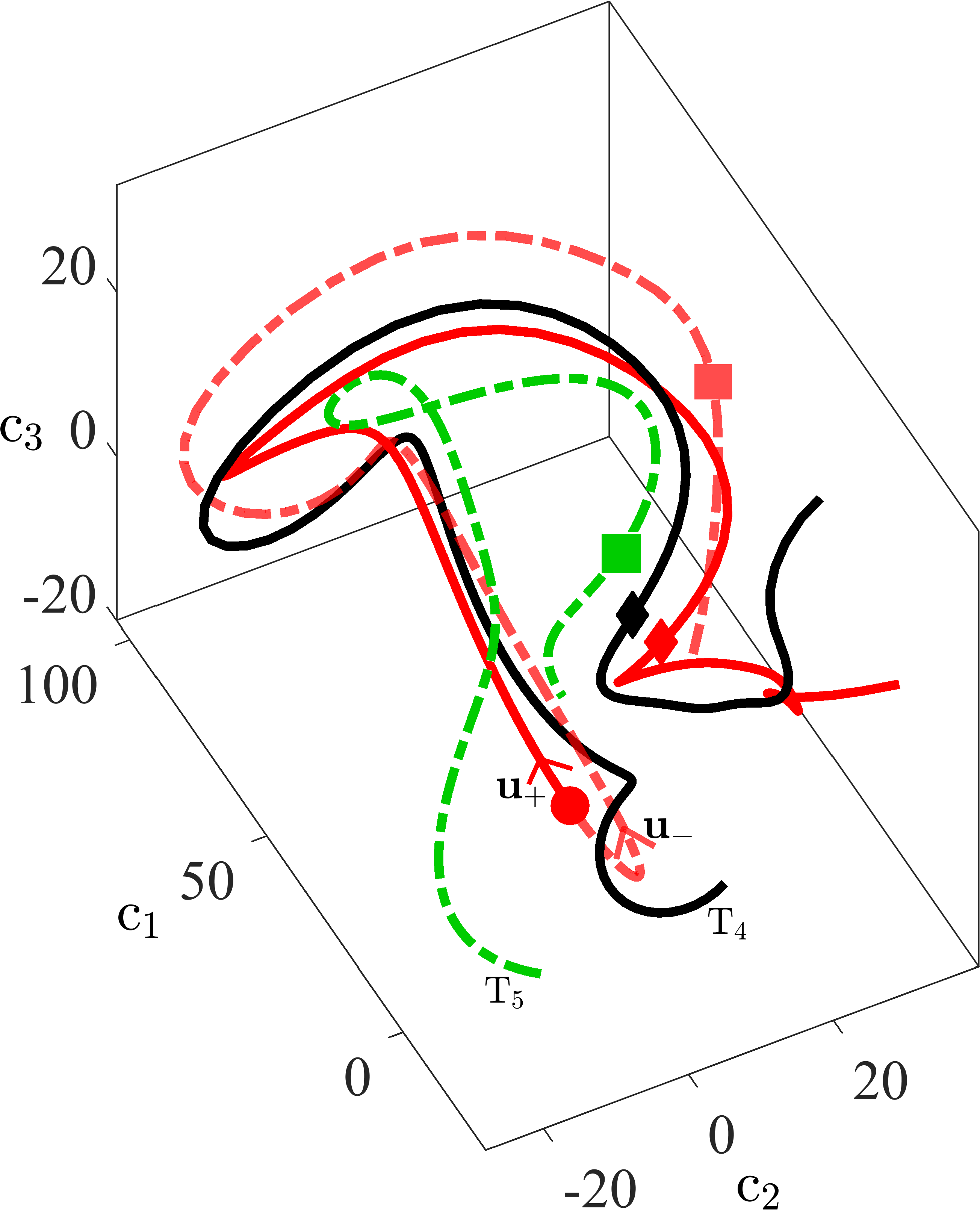
Figure 13: The dominant unstable submanifold ${\bf u}_{+}(t^{\prime})$ (solid red) and ${\bf u}_{-}(t^{\prime})$ (dashed red) of equilibrium E03 (red sphere). Also shown are turbulent trajectories from simulation ($\textrm{T}_{4}$ in black) and experiment ($\textrm{T}_{5}$ in green) that shadow ${\bf u}_{+}(t^{\prime})$ and ${\bf u}_{-}(t^{\prime})$, respectively. Details of the projection coordinates are provided in Appendix A.

Equilibrium E03 has a seven-dimensional unstable manifold with a leading real eigenvalue $\lambda_{1}$ = 0.1492 and three pairs of unstable complex conjugate eigenvalues $\lambda_{2,3}=0.0147\pm 0.1680i$, $\lambda_{4,5}=0.0045\pm 0.1104i$, and $\lambda_{6,7}=0.0009\pm 0.4500i$. Due to its relatively high dimensionality, constructing the corresponding unstable manifold is exceedingly data intensive. However, the spectral gap between the eigenvalues implies that not all unstable degrees of freedom are equally important dynamically Gibson et al. (2008); Halcrow et al. (2009). Trajectories starting from generic initial conditions close to E03 should quickly align in the direction of the leading eigenvector $\pm{\,\bf\hat{e}}_{1}$ (the corresponding perturbation in the physical space is shown in Appendix A).

The strong focusing effect implies that the dynamically relevant portion of the unstable manifold of E03 is effectively one-dimensional (1D) and is shaped by the pair of trajectories ${\bf u}_{\pm}(t^{\prime})$ departing from E03 along $\pm{\,\bf\hat{e}}_{1}$. The union of these two trajectories, which will be referred to as the dominant unstable submanifold in the following discussion, is shown as solid and dashed red curves in figure 13. Also shown are E03 (red sphere) and turbulent trajectories from simulation ($\textrm{T}_{4}$) and experiment ($\textrm{T}_{5}$) in its neighborhood. The figure is a projection of the state space onto an orthogonal basis constructed using ${\,\bf\hat{e}}_{1}$ and the eigenvectors ${\,\bf\hat{e}}_{6}$ and ${\,\bf\hat{e}}_{7}$ associated with the complex conjugate eigenvalue pair $\lambda_{6,7}$ (cf. Appendix A). It is interesting to point out that ${\bf u}_{+}(t^{\prime})$ appears nearly straight even well outside of the linear neighborhood of E03, while ${\bf u}_{-}(t^{\prime})$, which is initially oriented in the opposite direction, turns around not far from the equilibrium and starts following ${\bf u}_{+}(t^{\prime})$. This somewhat odd observation is not an artifact of the projection, as confirmed by the evolution of the corresponding flow fields in the physical space, which appear quite similar for an extended period of time.

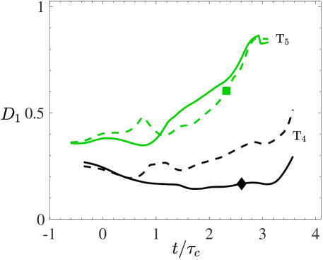
Figure 14: Distance $D_{1}(t)$ from turbulent trajectories ${\bf u}(t)$ in simulation ($\textrm{T}_{4}$) and experiment ($\textrm{T}_{5}$) to the 1D submanifold. Solid (dashed) curves correspond to distance from ${\bf u}_{+}(t^{\prime})$ (${\bf u}_{-}(t^{\prime})$). The diamond and square highlight separation between states indicated using the same symbols in figure 13.

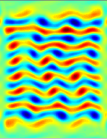
(a)

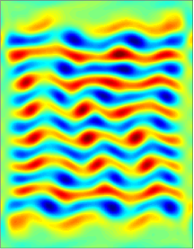
(b)

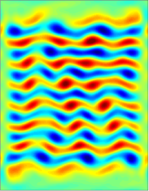
(c)

(d)

Figure 15: Comparison of flow fields far from E03. States on 1D submanifold trajectories (a) ${\bf u}_{+}(t^{\prime}_{m})$, marked using red diamond in figure 13 and (c) ${\bf u}_{-}(t^{\prime}_{m})$ (red square). Turbulent flow fields ${\bf u}(t_{m})$ from (b) simulation (black diamond on $\textrm{T}_{4}$) and (d) experiment (green square on $\textrm{T}_{5}$).

Both turbulent trajectories shown in figure 13 follow the 1D submanifold quite closely in the full state space, as the plot of the distance $D_{1}(t)$ shown in figure 14 illustrates. In particular, the numerical trajectory follows ${\bf u}_{+}(t^{\prime})$ with $D_{1}\leq 0.3$ along the entire interval $-0.5\tau_{c}\lesssim t\lesssim 3.5\tau_{c}$ shown in figure 13. Note that, once again, we set $t=0$ at the instant when $s(t)$ achieves a minimum for each of the turbulent trajectories visiting the neighborhood of E03. The experimental trajectory follows the 1D submanifold over a shorter interval $-0.5\tau_{c}\lesssim t\lesssim 2.5\tau_{c}$, after which it diverges from the submanifold as indicated by the value of $D_{1}$ exceeding our empiric threshold of 0.6. Notice that ${\bf u}(t)$ initially follows ${\bf u}_{+}(t^{\prime})$, but at $t\approx\tau_{c}$ it switches and starts following ${\bf u}_{-}(t^{\prime})$. At that point ${\bf u}_{+}(t^{\prime})$ and ${\bf u}_{-}(t^{\prime})$ are themselves quite close.

To illustrate how well the 1D submanifold reproduces turbulent dynamics far away from E03, we compare in figure 15(a) and (b) the flow field at the instant $t^{\prime}_{m}$ marked using the red diamond on ${\bf u}_{+}(t^{\prime}_{m})$ in figure 13 with the nearest point (black diamond) on the turbulent trajectory ${\bf u}(t_{m})$ from simulation. Similar comparison between ${\bf u}_{-}(t^{\prime}_{m})$ and ${\bf u}(t_{m})$ in experiment (red and green squares in figure 13) is shown in figure 15(c) and (d). The instant $t_{m}$ for each turbulent trajectory corresponds to the smaller of the distances

$$D^{\pm}_{1}=\min_{t}\frac{\|{\bf u}(t)-{\bf u}_{\pm}(t^{\prime}_{m})\|}{\|{\bf u}(t)\|}$$ (10)

from ${\bf u}(t)$ to ${\bf u}_{\pm}(t^{\prime}_{m})$.

These flow fields associated with ${\bf u}_{\pm}(t^{\prime}_{m})$ in the physical space are significantly different from that associated with E03 (cf. figure 12), confirming that ${\bf u}_{\pm}(t^{\prime}_{m})$ are far away from E03 in state space. This can be quantified more directly in terms of the distance to ${\bf u}_{\pm}(t^{\prime}_{m})$ along the submanifold, defined as an arc length in state space

$$D_{m}=\frac{1}{\|{\bf u}_{0}\|}\int_{-\infty}^{t^{\prime}_{m}}\left\|\frac{d{\bf u}_{\pm}(t^{\prime})}{dt^{\prime}}\right\|{dt^{\prime}}\approx\frac{1}{\tau_{c}}\int_{-\infty}^{t^{\prime}_{m}}s(t^{\prime})dt^{\prime},$$ (11)

where ${\bf u}_{0}={\bf u}_{\pm}(-\infty)$ is the equilibrium. The corresponding distances $D_{m}\approx 2.16$ for ${\bf u}_{+}(t^{\prime}_{m})$ (red diamond) and $D_{m}\approx 2.3$ for ${\bf u}_{-}(t^{\prime}_{m})$ (red square) are substantially larger than the empiric limit of $D_{0}\approx 0.6$ for closeness in state space. Hence we can conclude that the submanifold guides the evolution of these turbulent trajectories over large distances in the full state space, not just in its low-dimensional projection shown in figure 13.

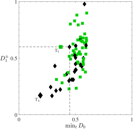
Figure 16: Distances from turbulent trajectories to the 1D submanifold. Axes $\min_{t}D_{0}(t)$ and $D^{\pm}_{1}$ are the minimum distances to E03 and ${\bf u}_{\pm}(t^{\prime}_{m})$, respectively. Diamonds ($D_{1}^{+}$) and squares ($D_{1}^{-}$) indicate closeness to ${\bf u}_{+}$ and ${\bf u}_{-}$, respectively.

In the discussion so far, we have demonstrated the dynamical role of the 1D submanifold using a pair of turbulent trajectories, one in simulation and the other in experiment, that approach E03 the closest. In fact, we found that all turbulent trajectories that come sufficiently close to this equilibrium always depart following its 1D submanifold. In the numerical simulations, we identified about 75 distinct instances when turbulent trajectories came within a distance $D_{0}\leq 0.6$ of E03. To check whether each trajectory follows the 1D submanifold after it leaves the neighborhood of E03, we compute the distances $D^{\pm}_{1}$ to the reference points ${\bf u}_{+}(t^{\prime}_{m})$ (red diamond) and ${\bf u}_{-}(t^{\prime}_{m})$ (red square). Comparing these distances, we can identify whether a turbulent trajectory follows ${\bf u}_{+}$ or ${\bf u}_{-}$.

Figure 16 shows $D^{\pm}_{1}$ for each of the 75 trajectories versus $\min_{t}D_{0}(t)$. Following the notations of figures 13 and 14, we use black diamonds (green squares) to indicate that ${\bf u}(t)$ follows ${\bf u}_{+}$ (${\bf u}_{-}$). For reference, $D_{1}^{+}$ ($D_{1}^{-}$) corresponding to the trajectory $\textrm{T}_{4}$ ($\textrm{T}_{5}$) is labeled in figure 16. All trajectories that approach E03 within a distance $D_{0}\leq 0.45$ follow the 1D submanifold quite closely, with $D^{\pm}_{1}\leq 0.6$. Hence, although the 1D submanifold is not locally attracting, it shapes the geometry of a relatively large region of state space around E03. Even for $D_{0}\geq 0.45$, a large fraction of turbulent trajectories still follows the 1D submanifold ($D^{\pm}_{1}\leq 0.6$); however the submanifold stops being a reliable predictor of the evolution.

V Conclusions

A vast majority of studies investigating fluid turbulence from a dynamical systems perspective have focused on the role of ECSs – mainly unstable traveling waves and time-periodic states – in the transition between laminar flow and turbulence, primarily using numerical simulations. In comparison, the dynamical role of other types of invariant sets (e.g., equilibria and stable/unstable manifolds associated with different ECSs) in turbulent evolution has received very little attention. Our combined experimental and numerical investigation of a canonical two-dimensional flow suggests that these invariant sets are important themselves.

Specifically, we found that unstable equilibria are responsible for the frequently observed slowdowns in the evolution of a weakly turbulent flow, making their presence felt far outside of their linear neighborhoods. On the other hand, no dynamically relevant time-periodic solutions with periods of up to 30 correlation times were found, despite a thorough and systematic search. By computing how closely turbulent trajectories approach each equilibrium, we have also determined that at least 27 of the 31 equilibria that we have computed are dynamically relevant, marking the first time a key piece of the dynamical systems approach has been directly validated in an experimental setting.

While equilibria themselves, being point-like objects in the state space, cannot shape the geometry of the chaotic set underpinning fluid turbulence, the associated stable and unstable manifolds do. We have demonstrated that unstable manifolds guide the evolution of turbulent flows that happen to pass through rather large neighborhoods of the corresponding equilibria, which makes these manifolds important building blocks in the deterministic, geometrical description of turbulence.

In particular, unstable manifolds associated with the dynamically dominant equilibria are relatively low-dimensional, which substantially constrains the shape of trajectories in their vicinity. The evolution can be constrained even further for unstable manifolds with a leading eigenvalue which is well-separated from the rest. As an example, we have shown that several turbulent trajectories entering the neighborhood of an equilibrium with a seven-dimensional unstable manifold depart following a one-dimensional submanifold associated with the leading eigenvector.

The dynamical role of stable manifolds of equilibria has not been discussed in any detail in the present study. They do appear to play an important role, however. A recent numerical study of channel flow has shown that the hairpin vortices – perhaps the most recognizable example of coherent structures in wall-bounded turbulent fluid flows – actually arise due to transient amplification of small, but finite-amplitude, disturbances in the stable manifold associated with a traveling wave solution (relative equilibrium) Farano et al. (2018). This intriguing result suggests that a more rigorous exploration of the role of stable manifolds is necessary for a better understanding of state space geometry.

The shape of both stable and unstable manifolds plays a key role in generating the chaotic dynamics underpinning turbulence. Heteroclinic tangles of stable and unstable manifolds of different ECSs are responsible for the stretching and folding of state space volumes that is an essential mechanism of chaos. On the other hand, intersections of stable and unstable manifolds of different ECSs define the heteroclinic connections, which connect neighborhoods of different ECSs and are expected to guide and constrain the evolution of turbulent flow as it moves between these neighborhoods. While the role of heteroclinic connections in fluid turbulence has also received little attention, they could potentially provide as much insight into the inner workings of turbulence as ECSs do. The present study is but a first step in computing and understanding the dynamical role of these underappreciated invariant sets.

Appendix A State Space Projections

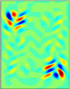
(a)

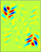
(b)

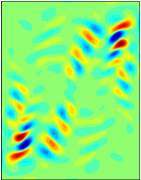
(c)

Figure 17: Eigenvectors of E01 used to construct the 3D projection of the state space shown in figure 7: (a) ${\,\bf\hat{e}}_{1}$, (b) ${\,\bf\hat{e}}_{2}$, (c) ${\,\bf\hat{e}}_{5}$.

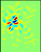
(a)

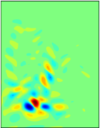
(b)

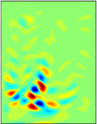
(c)

Figure 18: Eigenvectors of E03 used to construct the 3D projection of the state space shown in figure 12: (a) ${\,\bf\hat{e}}_{1}$, (b) $({\,\bf\hat{e}}_{6}+{\,\bf\hat{e}}_{7})/2$, (c) $({\,\bf\hat{e}}_{6}-{\,\bf\hat{e}}_{7})/(2i)$.

In this appendix, we provide details on constructing state space visualizations in figures 7 and 13. Near an equilibrium ${\bf u}_{0}$, we express the turbulent and manifold trajectories in state space as a linear combination of the eigenvectors ${\,\bf\hat{e}}_{k}$ of the equilibrium:

$${\bf u}(t)={\bf u}_{0}+\sum_{k}a_{k}{\,\bf\hat{e}}_{k}$$ (12)

Typically, eigenvectors ${\,\bf\hat{e}}_{k}$ are not mutually orthogonal, i.e., ${\,\bf\hat{e}}_{k}\cdot{\,\bf\hat{e}}_{l}\neq\delta_{k,l}$, where $\delta_{k,l}$ is the Kronecker delta. Hence, coordinates $a_{k}$ are given by using the scalar product

$$a_{k}={\,\bf\hat{e}}_{k}^{\dagger}\cdot({\bf u}(t)-{\bf u}_{0})$$ (13)

with adjoint eigenvectors ${\,\bf\hat{e}}_{k}^{\dagger}$ such that ${\,\bf\hat{e}}_{k}^{\dagger}\cdot{\,\bf\hat{e}}_{l}=\delta_{k,l}$. To project the state space onto a subspace spanned by any three eigenvectors ${\,\bf\hat{e}}_{k},{\,\bf\hat{e}}_{l},{\,\bf\hat{e}}_{m}$, we construct orthonormal vectors ${\,\bf\hat{e}}^{\prime}_{k}=T_{kl}{\,\bf\hat{e}}_{l}$. Here, $T_{kl}$ is computed using the orthonormality condition ${\,\bf\hat{e}}^{\prime}_{k}\cdot{\,\bf\hat{e}}^{\prime}_{l}=\delta_{k,l}$. The coordinates

$$c_{k}=T_{kl}a_{l}$$ (14)

along vectors ${\,\bf\hat{e}}^{\prime}_{k}$ are then used to generate the projection figures.

The choice of the three eigenvectors is guided by their dynamical relevance as well as the amplitudes $a_{k}$ of nearby turbulent trajectories. In particular, the 2D unstable manifold of E01 shown in figure 7 is locally tangent to the plane spanned by ${\,\bf\hat{e}}_{1}$ and ${\,\bf\hat{e}}_{2}$, so these two eigenvectors are a natural choice. For the third direction, we chose the stable eigenvector ${\,\bf\hat{e}}_{5}$, since the manifold trajectories far away from E01 tend to have large components along ${\,\bf\hat{e}}_{5}$. This proved useful in showcasing the curvature of the unstable manifold. The shapes of ${\,\bf\hat{e}}_{1}$, ${\,\bf\hat{e}}_{2}$, and ${\,\bf\hat{e}}_{5}$ in the physical space are shown in figure 17.

In the neighborhood of E03 (cf. figure 13), we project the state space onto a basis spanned by the leading unstable eigenvector ${\,\bf\hat{e}}_{1}$ and the eigenvectors ${\,\bf\hat{e}}_{6}$, ${\,\bf\hat{e}}_{7}$ associated with the complex conjugate eigenvalue pair $\lambda_{6}=\lambda_{7}^{*}$. Like in the 2D manifold example, eigenvectors ${\,\bf\hat{e}}_{6}$, ${\,\bf\hat{e}}_{7}$ were chosen because they well represent the curvature of the 1D submanifold away from E03. The shapes of ${\,\bf\hat{e}}_{1}$ and the real and complex parts of ${\,\bf\hat{e}}_{6},{\,\bf\hat{e}}_{7}$ in physical space are shown in figure 18.

Appendix B Temporal Autocorrelation

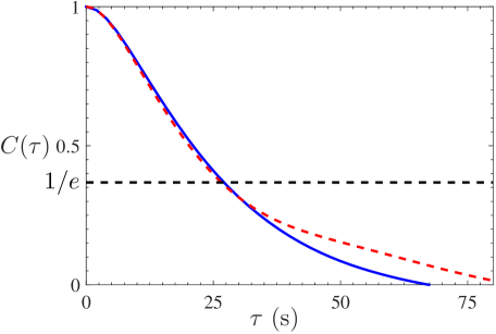
Figure 19: Temporal auto-correlation of the velocity field at $Re=22.5$. The solid (dashed) curve corresponds to simulation (experiment).

The estimate for how long it typically takes for a turbulent flow field to change significantly in the course of its evolution can be obtained from the temporal auto-correlation of the velocity field:

$$C(\tau)=\frac{\langle\Delta{\bf u}(t)\cdot\Delta{\bf u}(t+\tau)\rangle_{t}}{\langle\Delta{\bf u}(t)\cdot\Delta{\bf u}(t)\rangle_{t}},$$ (15)

where $\langle\cdot\rangle_{t}$ indicates temporal average, $\Delta{\bf u}(t)={\bf u}(t)-\langle{\bf u}(t)\rangle_{t}$, and the scalar product of two fields ${\bf u}$ and ${\bf v}$ is defined as

$${\bf u}\cdot{\bf v}=\sum_{i=x,y}\int_{\Omega}u_{i}({\bf x})v_{i}({\bf x})d^{2}{\bf x},$$ (16)

where $\Omega$ is the flow domain.

Figure 19 shows a plot of the normalized temporal auto-correlation as a function of $\tau$ at $Re=22.5$. The normalization criterion $C(0)=1$, takes into account that a flow field at every instant is identical (and hence perfectly correlated) to itself. The correlation time $\tau_{c}$ can be defined as the smallest root of $C(\tau)=1/e$, denoted by the black dashed line in figure 19. For the simulation as well as the experiment the correlation time $\tau_{c}\approx 12.5$ ($27\pm 1$ s in dimensional units).

References

- Hopf (1948) E. Hopf, Commun. Pur. Appl. Math. 1, 303 (1948).
- Landau and Lifshitz (1959) L. D. Landau and E. M. Lifshitz, Fluid Mechanics (Pergamon, 1959).
- Arnold (2009) V. I. Arnold, Vladimir I. Arnold - Collected Works: Representations of Functions, Celestial Mechanics, and KAM Theory 1957–1965 (Springer, 2009) pp. 423–427.
- Auerbach et al. (1987) D. Auerbach, P. Cvitanović, J. P. Eckmann, G. Gunaratne, and I. Procaccia, Phys. Rev. Lett. 58, 23 (1987).
- Cvitanović (1988) P. Cvitanović, Phys. Rev. Lett. 61, 2729 (1988).
- Lorenz (1963) E. N. Lorenz, J. Atmos. Sci. 20, 130 (1963).
- Poincaré (1993) H. Poincaré, New methods of celestial mechanics (Springer, 1993).
- Saad and Schultz (1986) Y. Saad and M. H. Schultz, SIAM J. Sci. Stat. Comp. 7, 856 (1986).
- Kelley (1995) C. Kelley, Iterative Methods for Linear and Nonlinear Equations (Society for Industrial and Applied Mathematics, 1995).
- Gibson et al. (2008) J. F. Gibson, J. Halcrow, and P. Cvitanović, J. Fluid Mech. 611, 107 (2008).
- Cvitanović and Gibson (2010) P. Cvitanović and J. F. Gibson, Phys. Scripta 2010, 014007 (2010).
- Suri et al. (2017) B. Suri, J. Tithof, R. O. Grigoriev, and M. F. Schatz, Phys. Rev. Lett. 118, 114501 (2017).
- Kerswell and Tutty (2007) R. R. Kerswell and O. R. Tutty, J. Fluid Mech. 584, 69–102 (2007).
- Wang et al. (2007) J. Wang, J. Gibson, and F. Waleffe, Phys. Rev. Lett. 98, 204501 (2007).
- Budanur et al. (2017a) N. B. Budanur, K. Y. Short, M. Farazmand, A. P. Willis, and P. Cvitanović, J. Fluid Mech. 833, 274–301 (2017a).
- Schneider et al. (2017) T. M. Schneider, M. Farano, P. D. Palma, J.-C. Robinet, and S. Cherubini (2017) http://meetings.aps.org/link/BAPS.2017.DFD.L1.8.
- Farano et al. (2018) M. Farano, S. Cherubini, P. D. Palma, J.-C. Robinet, and T. M. Schneider, Phys. Rev. Lett. (2018), under review.
- Halcrow et al. (2009) J. Halcrow, J. F. Gibson, P. Cvitanović, and D. Viswanath, J. Fluid Mech. 621, 365 (2009).
- Riols et al. (2013) A. Riols, F. Rincon, C. Cossu, G. Lesur, P.-Y. Longaretti, G. I. Ogilvie, and J. Herault, Journal of Fluid Mechanics 731, 1 (2013).
- Nagata (1997) M. Nagata, Phys. Rev. E 55, 2023 (1997).
- Waleffe (2001) F. Waleffe, J. Fluid Mech. 435, 93 (2001).
- Faisst and Eckhardt (2003) H. Faisst and B. Eckhardt, Phys. Rev. Lett. 91, 224502 (2003).
- Wedin and Kerswell (2004) H. Wedin and R. Kerswell, J. Fluid Mech. 508, 333 (2004).
- Hamilton et al. (1995) J. M. Hamilton, J. Kim, and F. Waleffe, J. Fluid Mech. 287 (1995).
- Kline et al. (1967) S. Kline, W. Reynolds, F. Schraub, and P. Runstadler, J. Fluid Mech. 30, 741 (1967).
- Kawahara and Kida (2001) G. Kawahara and S. Kida, J. Fluid Mech. 449, 291 (2001).
- Viswanath (2007) D. Viswanath, J. Fluid Mech. 580, 339 (2007).
- Waleffe (1997) F. Waleffe, Phys. Fluids 9, 883 (1997).
- Schneider et al. (2007a) T. M. Schneider, B. Eckhardt, and J. A. Yorke, Phys. Rev. Lett. 99, 034502 (2007a).
- Hof et al. (2004) B. Hof, C. W. H. van Doorne, J. Westerweel, F. T. M. Nieuwstadt, H. Faisst, B. Eckhardt, H. Wedin, R. R. Kerswell, and F. Waleffe, Science 305, 1594 (2004).
- de Lozar et al. (2012) A. de Lozar, F. Mellibovsky, M. Avila, and B. Hof, Phys. Rev. Lett. 108, 214502 (2012).
- Dennis and Sogaro (2014) D. J. C. Dennis and F. M. Sogaro, Phys. Rev. Lett. 113, 234501 (2014).
- Lemoult et al. (2014) G. Lemoult, K. Gumowski, J.-L. Aider, and J. E. Wesfreid, Eur. Phys. J. E 37, 1 (2014).
- Schneider et al. (2007b) T. M. Schneider, B. Eckhardt, and J. Vollmer, Phys. Rev. E 75, 066313 (2007b).
- Kerswell (2005) R. R. Kerswell, Nonlinearity 18, R17 (2005).
- Eckhardt (2009) B. Eckhardt, Philos. T. R. Soc. A 367, 449 (2009).
- Itano and Toh (2001) T. Itano and S. Toh, J. Phys. Soc. Jpn. 70, 703 (2001).
- Viswanath and Cvitanovic (2009) D. Viswanath and P. Cvitanovic, J. Fluid Mech. 627, 215–233 (2009).
- Budanur and Hof (2018) N. B. Budanur and B. Hof, Phys. Rev. Fluids 3, 054401 (2018).
- Toh and Itano (2003) S. Toh and T. Itano, J. Fluid Mech. 481, 67–76 (2003).
- Kawahara (2005) G. Kawahara, Phys. Fluids 17, 041702 (2005).
- Duguet et al. (2008) Y. Duguet, C. C. T. Pringle, and R. R. Kerswell, Phys. Fluids 20, 114102 (2008).
- Van Heijst and Clercx (2009) G. J. F. Van Heijst and H. J. H. Clercx, Annu. Rev. Fluid Mech. 41, 143 (2009).
- Dolzhansky (2013) F. V. Dolzhansky, Fundamentals of Geophysical Hydrodynamics, Encyclopaedia of Mathematical Sciences, Vol. 103 (Springer, 2013) p. 266, translated by B. A. Khesin.
- Suri et al. (2014) B. Suri, J. Tithof, R. Mitchell, R. O. Grigoriev, and M. F. Schatz, Phys. Fluids 26, 053601 (2014).
- Meshalkin and Sinai (1961) L. D. Meshalkin and I. G. Sinai, J. Appl. Math. Mech. 25, 1700 (1961).
- Chandler and Kerswell (2013) G. J. Chandler and R. R. Kerswell, J. Fluid Mech. 722, 554 (2013).
- Drew et al. (2013) B. Drew, J. Charonko, and P. P. Vlachos, “QI – Quantitative Imaging (PIV and more),” (2013), available at https://sourceforge.net/projects/qi-tools/.
- Satijn et al. (2001) M. P. Satijn, A. W. Cense, R. Verzicco, H. J. H. Clercx, and G. J. F. van Heijst, Phys. Fluids 13, 1932 (2001).
- Tithof et al. (2017) J. Tithof, B. Suri, R. K. Pallantla, R. O. Grigoriev, and M. F. Schatz, J. Fluid Mech. 828, 837 (2017).
- LeVeque and Leveque (1992) R. J. LeVeque and R. J. Leveque, Numerical methods for conservation laws, Vol. 132 (Springer, 1992).
- Griebel et al. (1998) M. Griebel, T. Dornseifer, and T. Neunhoeffer, Numerical Simulation in Fluid Dynamics (SIAM, 1998).
- van Kan (1986) J. van Kan, SIAM J. Sci. Stat. Comp. 7, 870 (1986).
- Armfield and Street (1999) S. Armfield and R. Street, J. Comput. Phys. 153, 660 (1999).
- Suri (2017) B. Suri, Quasi-Two-Dimensional Kolmogorov flow: Bifurcations and Exact Coherent Structures, Ph.D. thesis, Georgia Institute of Technology (2017).
- Cvitanović (2013) P. Cvitanović, J. Fluid Mech. 726, 1 (2013).
- Budanur et al. (2017b) N. B. Budanur, K. Y. Short, M. Farazmand, A. P. Willis, and P. Cvitanović, J. Fluid Mech. 833, 274–301 (2017b).
- Eckmann et al. (1987) J.-P. Eckmann, S. O. Kamphorst, and D. Ruelle, Europhys. Lett. 4, 973 (1987).
- Neelavara et al. (2017) S. A. Neelavara, Y. Duguet, and F. Lusseyran, Fluid Dynamics Research 49, 035511 (2017).
- Kelley (2003) C. Kelley, Solving Nonlinear Equations with Newton’s Method (SIAM, 2003).
- Mitchell (2013) R. Mitchell, Transition to turbulence and mixing in a quasi-two-dimensional Lorentz force-driven Kolmogorov flow, Ph.D. thesis, Georgia Institute of Technology (2013).
- Farazmand (2016) M. Farazmand, J. Fluid Mech. 795, 278–312 (2016).
- Ruelle and Takens (1971) D. Ruelle and F. Takens, Commun. Math. Phys. 20, 167 (1971).
- Brandstäter et al. (1983) A. Brandstäter, J. Swift, H. L. Swinney, A. Wolf, J. D. Farmer, E. Jen, and P. J. Crutchfield, Phys. Rev. Lett. 51, 1442 (1983).
- Farmer et al. (1983) J. Farmer, E. Ott, and J. A. Yorke, Physica D: Nonlinear Phenomena 7, 153 (1983).
- Christiansen and Rugh (1997) F. Christiansen and H. H. Rugh, Nonlinearity 10, 1063 (1997).