Abstract

We develop unbiased implicit variational inference (uivi), a method that expands the applicability of variational inference by defining an expressive variational family. uivi considers an implicit variational distribution obtained in a hierarchical manner using a simple reparameterizable distribution whose variational parameters are defined by arbitrarily flexible deep neural networks. Unlike previous works, uivi directly optimizes the evidence lower bound (elbo)rather than an approximation to the elbo. We demonstrate uivi on several models, including Bayesian multinomial logistic regression and variational autoencoders, and show that uivi achieves both tighter elbo and better predictive performance than existing approaches at a similar computational cost.

1 INTRODUCTION

Variational inference (vi) is an approximate Bayesian inference technique that recasts inference as an optimization problem (Jordan, 1999; Wainwright & Jordan, 2008; Blei et al., 2017). The goal of vi is to approximate the posterior $p(z\,|\,x)$ of a given probabilistic model $p(x,z)$, where $x$ denotes the data and $z$ stands for the latent variables. vi posits a parameterized family of distributions $q_{\theta}(z)$ and then minimizes the Kullback-Leibler (kl) divergence between the approximating distribution $q_{\theta}(z)$ and the exact posterior $p(z\,|\,x)$. This minimization is equivalent to maximizing the evidence lower bound (elbo), which is a function $\mathcal{L}(\theta)$ expressed as an expectation over the variational distribution,

$$\mathcal{L}(\theta)=\mathbb{E}_{q_{\theta}(z)}\left[\log p(x,z)-\log q_{\theta}(z)\right].$$ (1)

Thus, vi maximizes Eq. 1, which involves the log-joint $\log p(x,z)$ rather than the intractable posterior.

Classical vi relies on the assumption that the expectations in Eq. 1 are tractable and applies a coordinate-wise ascent algorithm to find $\theta$ (Ghahramani & Beal, 2001). In general, this assumption requires two conditions: the model must be conditionally conjugate (meaning that the conditionals $p(z_{n}\,|\,x,z_{\neg n})$ are in the same exponential family as the prior $p(z_{n})$ for each latent variable $z_{n}$), and the variational family must have a simplified form such as to be factorized across latent variables (mean-field vi).

The above two restrictive conditions when applying vi have motivated several lines of research to expand the use of vi to more complex settings. To address the conjugacy condition on the model, black-box vi methods have been developed, allowing vi to be applied on a broad class of models by using Monte Carlo estimators of the gradient (Carbonetto et al., 2009; Paisley et al., 2012; Ranganath et al., 2014; Kingma & Welling, 2014; Rezende et al., 2014; Titsias & Lázaro-Gredilla, 2014; Kucukelbir et al., 2015, 2017). To address the simplified (typically mean-field) form of the variational family, more complex variational families have been proposed that incorporate some structure among the latent variables (Jaakkola & Jordan, 1998; Saul & Jordan, 1996; Giordano et al., 2015; Tran et al., 2015, 2016; Ranganath et al., 2016; Han et al., 2016; Maaløe et al., 2016). See also Zhang et al. (2017) for a review on recent advances on variational inference.

Here, we focus on implicit vi where the variational distribution $q_{\theta}(z)$ can have arbitrarily flexible forms constructed using neural network mappings. A distribution $q_{\theta}(z)$ is implicit when it is not possible to evaluate its density but it is possible to draw samples from it. One typical way to draw from an implicit distribution in vi is to first sample a noise vector and then push it through a deep neural network (Mohamed & Lakshminarayanan, 2016; Huszár, 2017; Tran et al., 2017; Li & Turner, 2018; Mescheder et al., 2017; Shi et al., 2018a). Implicit vi expands the variational family making $q_{\theta}(z)$ more expressive, but computing $\log q_{\theta}(z)$ in Eq. 1—or its gradient—becomes intractable. To address that, implicit vi typically relies on density ratio estimation. However, density ratio estimation is challenging in high-dimensional settings. To avoid density ratio estimation, Yin & Zhou (2018) proposed semi-implicit variational inference (sivi), an approach that obtains the variational distribution $q_{\theta}(z)$ by mixing the variational parameter with an implicit distribution. Exploiting this definition of $q_{\theta}(z)$, sivi optimizes a sequence of lower (or upper) bounds on the elbo that eventually converge to Eq. 1.

In this paper, we develop an unbiased estimator of the gradient of the elbo that avoids density ratio estimation. Our approach builds on sivi in that we also define the variational distribution by mixing the variational parameter with an implicit distribution. In contrast to sivi, we propose an unbiased optimization method that directly maximizes the elbo rather than a bound. We call our method unbiased implicit variational inference (uivi). We show experimentally that uivi can achieve better elbo and predictive log-likelihood than sivi at a similar computational cost.

We develop uivi using a semi-implicit variational approximation $q_{\theta}(z)=\int q_{\theta}(z\,|\,\varepsilon)q(\varepsilon)d\varepsilon$, such that the conditional $q_{\theta}(z\,|\,\varepsilon)$ is a reparameterizable distribution. The dependence of the conditional $q_{\theta}(z\,|\,\varepsilon)$ on the random variable $\varepsilon$ can be arbitrarily complex. We use a deep neural network parameterized by $\theta$ that takes $\varepsilon$ as input and outputs the parameters of the conditional $q_{\theta}(z\,|\,\varepsilon)$. Given $\varepsilon$, the conditional is a “simple” reparameterizable distribution; however marginalizing out $\varepsilon$ results in an implicit and more complex distribution $q_{\theta}(z)$. Exploiting these properties of the variational distribution, uivi expresses the gradient of the elbo in Eq. 1 as an expectation, allowing us to construct an unbiased Monte Carlo estimator. The resulting estimator requires samples from the conditional distribution $q_{\theta}(\varepsilon\,|\,z)\propto q_{\theta}(z\,|\,\varepsilon)q(\varepsilon)$. We develop a computationally efficient way to draw samples from this conditional using a fast Markov chain Monte Carlo (mcmc) procedure that starts from the stationary distribution. In this way, we avoid the time-consuming burn-in or transient phase that characterizes mcmc methods.

2 UNBIASED IMPLICIT VARIATIONAL INFERENCE

In this section we present unbiased implicit variational inference (uivi). First, in Section 2.1 we describe how to build the variational distribution, following semi-implicit variational inference (sivi) (Yin & Zhou, 2018). Second, in Section 2.2 we show how to form an unbiased estimator of the gradient of the evidence lower bound (elbo). Finally, in Section 2.3 we put forward the resulting uivi algorithm and explain how to run it efficiently.

2.1 Semi-Implicit Variational Distribution

To approximate the posterior $p(z\,|\,x)$ of a probabilistic model $p(x,z)$, uivi uses a semi-implicit variational distribution $q_{\theta}(z)$ (Yin & Zhou, 2018). This means that $q_{\theta}(z)$ is defined in a hierarchical manner with a mixing parameter,

$$\varepsilon\sim q(\varepsilon),\quad z\sim q_{\theta}(z\,|\,\varepsilon),$$ (2)

or equivalently,

$$q_{\theta}(z)=\int q_{\theta}(z\,|\,\varepsilon)q(\varepsilon)d\varepsilon.$$ (3)

Eqs. 2 and 3 reveal why the resulting variational distribution $q_{\theta}(z)$ is implicit, as we can obtain samples from it (Eq. 2) but cannot evaluate its density, as the integral in Eq. 3 is intractable.

The dependence of the conditional $q_{\theta}(z\,|\,\varepsilon)$ on the random variable $\varepsilon$ can be arbitrarily complex. In uivi, its parameters are the output of a deep neural network (parameterized by the variational parameters $\theta$) that takes $\varepsilon$ as input.

Assumptions.  In uivi, the conditional $q_{\theta}(z\,|\,\varepsilon)$ must satisfy two assumptions. First, it must be reparameterizable. That is, to sample from $q_{\theta}(z\,|\,\varepsilon)$, we can first draw an auxiliary variable $u$ and then set $z$ as a deterministic function $h_{\theta}(\cdot)$ of the sampled $u$,

$$u\sim q(u),\;\;z=h_{\theta}(u\,;\,\varepsilon)\quad\equiv\quad z\sim q_{\theta}(z\,|\,\varepsilon).$$ (4)

The transformation $h_{\theta}(u\,;\,\varepsilon)$ is parameterized by the random variable $\varepsilon$ and the variational parameters $\theta$, but the auxiliary distribution $q(u)$ has no parameters. Figure 1 illustrates this construction of the variational distribution.

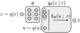
Figure 1: Illustration of the sampling procedure for the implicit variational distribution $q_{\theta}(z)$. First, a sample $\varepsilon\sim q(\varepsilon)$ is pushed through a neural network with parameters $\theta$ (left block). This network outputs the parameters (dotted ellipse) of the conditional distribution $q_{\theta}(z\,|\,\varepsilon)$. Since the conditional is reparameterizable (right block), to draw a sample $z$ we can first sample $u\sim q(u)$ and then set $z=h_{\theta}(u\,;\,\varepsilon)$, where $h_{\theta}(\cdot)$ is an appropriate transformation. The transformation $h_{\theta}(\cdot)$ depends on $\varepsilon$ and $\theta$ through the parameters of the conditional. The output $z=h_{\theta}(u\,;\,\varepsilon)$ is a sample from the variational distribution $q_{\theta}(z)$.

The second assumption on the conditional $q_{\theta}(z\,|\,\varepsilon)$ is that it is possible to evaluate the log-density $\log q_{\theta}(z\,|\,\varepsilon)$ and its gradient with respect to $z$, $\nabla_{z}\log q_{\theta}(z\,|\,\varepsilon)$. This is not a strong assumption; it holds for many reparameterizable distributions (e.g., Gaussian, Laplace, exponential, etc.).

uivi makes use of these two properties of the conditional $q_{\theta}(z\,|\,\varepsilon)$ to derive unbiased estimates of the gradient of the elbo (see Section 2.2).

Example: Gaussian conditional.  As a simple example, consider a multivariate Gaussian distribution for the conditional $q_{\theta}(z\,|\,\varepsilon)$. The parameters of the Gaussian are its mean $\mu_{\theta}(\varepsilon)$ and covariance $\Sigma_{\theta}(\varepsilon)$. Both parameters are given by neural networks with parameters $\theta$ and input $\varepsilon$.

The Gaussian meets the two assumptions outlined above. It is reparameterizable because it is in the location-scale family; the sampling process

$$\begin{split}&u\sim q(u)=\mathcal{N}(u\,|\,0,I),\\ &z=h_{\theta}(u\,;\,\varepsilon)=\mu_{\theta}(\varepsilon)+\Sigma_{\theta}(\varepsilon)^{1/2}u\end{split}$$

generates a sample $z\sim q_{\theta}(z\,|\,\varepsilon)$.

Furthermore, the Gaussian density and the gradient of the log-density can be evaluated. The latter is

$$\nabla_{z}\log q_{\theta}(z\,|\,\varepsilon)=-\Sigma_{\theta}(\varepsilon)^{-1}\left(z-\mu_{\theta}(\varepsilon)\right).$$

2.2 Unbiased Gradient Estimator

Here we derive the unbiased gradient estimators of the elbo. First, uivi uses the reparameterization $z=h_{\theta}(u\,;\,\varepsilon)$ (Eq. 4) to rewrite the expectation in Eq. 1 as an expectation with respect to $q(\varepsilon)$ and $q(u)$,

$$\mathcal{L}(\theta)=\mathbb{E}_{q(\varepsilon)q(u)}\left[\log p(x,z)-\log q_{\theta}(z)\Big{|}_{z=h_{\theta}(u\,;\,\varepsilon)}\right].$$

To obtain the gradient of the elbo with respect to $\theta$, the gradient operator can now be pushed inside the expectation, as in the standard reparameterization method (Kingma & Welling, 2014; Titsias & Lázaro-Gredilla, 2014; Rezende et al., 2014). This gives two terms: one corresponding to the model and one corresponding to the entropy,

$$\nabla_{\theta}\mathcal{L}(\theta)=\mathbb{E}_{q(\varepsilon)q(u)}\left[g_{\theta}^{\textrm{mod}}(\varepsilon,u)+g_{\theta}^{\textrm{ent}}(\varepsilon,u)\right].$$ (5)

The term corresponding to the model is

$$g_{\theta}^{\textrm{mod}}(\varepsilon,u)\triangleq\nabla_{z}\log p(x,z)\Big{|}_{z=h_{\theta}(u\,;\,\varepsilon)}\nabla_{\theta}h_{\theta}(u\,;\,\varepsilon);$$ (6)

similarly, the term corresponding to the entropy is

$$g_{\theta}^{\textrm{ent}}(\varepsilon,u)\triangleq-\nabla_{z}\log q_{\theta}(z)\Big{|}_{z=h_{\theta}(u\,;\,\varepsilon)}\nabla_{\theta}h_{\theta}(u\,;\,\varepsilon).$$ (7)

To obtain this decomposition, we have applied the identity that the expected value of the score function is zero, $\mathbb{E}_{q_{\theta}(z)}\left[\nabla_{\theta}\log q_{\theta}(z)\right]=0$, which reduces the variance of the estimator (Roeder et al., 2017).

uivi estimates the model component in Eq. 6 using samples from $q(\varepsilon)$ and $q(u)$. However, estimating the entropy component in Eq. 7 is harder because the term $\nabla_{z}\log q_{\theta}(z)$ cannot be evaluated—the variational distribution $q_{\theta}(z)$ is an implicit distribution.

uivi addresses this issue rewriting Eq. 7 as an expectation, therefore enabling Monte Carlo estimates of the entropy component of the gradient. In particular, uivi rewrites as an expectation the intractable log-density gradient in Eq. 7,

$$\nabla_{z}\log q_{\theta}(z)=\mathbb{E}_{q_{\theta}(\varepsilon\,|\,z)}\left[\nabla_{z}\log q_{\theta}(z\,|\,\varepsilon)\right].$$ (8)

We prove Eq. 8 below. This equation shows that the problematic gradient $\nabla_{z}\log q_{\theta}(z)$ can be expressed in terms of an expression that can be evaluated—the gradient of the log-conditional $\nabla_{z}\log q_{\theta}(z\,|\,\varepsilon)$ can be evaluated by assumption (see Section 2.1). uivi rewrites the entropy term in Eq. 7 using Eq. 8,

$$g_{\theta}^{\textrm{ent}}(\varepsilon,u)= -\mathbb{E}_{q_{\theta}(\varepsilon^{\prime}\,|\,z)}\left[\nabla_{z}\log q_{\theta}(z\,|\,\varepsilon^{\prime})\right]\Big{|}_{z=h_{\theta}(u\,;\,\varepsilon)}$$

$$\times\nabla_{\theta}h_{\theta}(u\,;\,\varepsilon).$$ (9)

(We use the notation $\varepsilon^{\prime}$ to make it explicit that this variable is different from $\varepsilon$.)

The expectation in Eqs. 8 and 9 is taken with respect to the distribution $q_{\theta}(\varepsilon\,|\,z)\propto q_{\theta}(z\,|\,\varepsilon)q(\varepsilon)$. We call this distribution the reverse conditional. Although the conditional $q_{\theta}(z\,|\,\varepsilon)$ has a simple form (by assumption, it is a reparameterizable distribution for which we can evaluate the density and its gradient), the reverse conditional is complex because the conditional $q_{\theta}(z\,|\,\varepsilon)$ is parameterized by deep neural networks that take $\varepsilon$ as input. We show in Section 2.3 how to efficiently draw samples from the reverse conditional to obtain an estimator of the entropy component in Eq. 9. (The main idea is to reuse a sample from the reverse conditional to initialize a sampler.)

We now prove Eq. 8 and then we show two examples that particularize these expressions for two choices of the conditionals: a multivariate Gaussian and a more general exponential family distribution.

Proof of Eq. 8.  We show how to express the gradient $\nabla_{z}\log q_{\theta}(z)$ as an expectation. We start with the log-derivative identity,

$$\nabla_{z}\log q_{\theta}(z)=\frac{1}{q_{\theta}(z)}\nabla_{z}q_{\theta}(z).$$

Next we use the definition of the semi-implicit distribution $q_{\theta}(z)$ through a mixing distribution (Eq. 3) and we push the gradient into the integral,

$$\begin{split}\nabla_{z}\log q_{\theta}(z)&=\frac{1}{q_{\theta}(z)}\nabla_{z}\int q_{\theta}(z\,|\,\varepsilon)q(\varepsilon)d\varepsilon\\ &=\frac{1}{q_{\theta}(z)}\int\nabla_{z}q_{\theta}(z\,|\,\varepsilon)q(\varepsilon)d\varepsilon.\end{split}$$

We now apply the log-derivative identity on the conditional $q_{\theta}(z\,|\,\varepsilon)$,

$$\begin{split}\nabla_{z}\log q_{\theta}(z)=\frac{1}{q_{\theta}(z)}\int q_{\theta}(z\,|\,\varepsilon)q(\varepsilon)\nabla_{z}\log q_{\theta}(z\,|\,\varepsilon)d\varepsilon.\end{split}$$

Finally, we apply Bayes’ theorem to obtain Eq. 8.       $\square$

Example: Gaussian conditional.  Consider the multivariate Gaussian example from Section 2.1. Substituting the gradient of the Gaussian log-density into Eq. 9, we can write the entropy component of the gradient as

$$g_{\theta}^{\textrm{ent}}(\varepsilon,u)= \;\mathbb{E}_{q_{\theta}(\varepsilon^{\prime}\,|\,z)}\left[\Sigma_{\theta}(\varepsilon^{\prime})^{-1}\left(z-\mu_{\theta}(\varepsilon^{\prime})\right)\right]\Big{|}_{z=h_{\theta}(u\,;\,\varepsilon)}$$

$$\times\nabla_{\theta}h_{\theta}(u\,;\,\varepsilon).$$

Example: Exponential family conditional.  Now consider the more general example of a reparameterizable exponential family conditional distribution $q_{\theta}(z\,|\,\varepsilon)$ with sufficient statistics $t(z)$ and natural parameter $\eta_{\theta}(\varepsilon)$,

$$q_{\theta}(z\,|\,\varepsilon)\propto\exp\{t(z)^{\top}\eta_{\theta}(\varepsilon)\}.$$ (10)

Substituting the gradient $\nabla_{z}\log q_{\theta}(z\,|\,\varepsilon)$ into Eq. 9, we can obtain the entropy component of the gradient for a general (reparameterizable) exponential family distribution,

$$g_{\theta}^{\textrm{ent}}(\varepsilon,u)= \;-\nabla_{z}t(z)^{\top}\mathbb{E}_{q_{\theta}(\varepsilon^{\prime}\,|\,z)}\left[\eta_{\theta}(\varepsilon^{\prime})\right]\Big{|}_{z=h_{\theta}(u\,;\,\varepsilon)}$$

$$\;\times\nabla_{\theta}h_{\theta}(u\,;\,\varepsilon).$$

2.3 Full Algorithm

uivi estimates the gradient of the elbo using Eq. 5, which decomposes the gradient as the expectation of the sum of the model component and the entropy component. uivi estimates the expectation using $S$ samples from $q(\varepsilon)$ and $q(u)$ ($S=1$ in practice); that is,

$$\nabla_{\theta}\mathcal{L}(\theta)\approx\frac{1}{S}\sum_{s=1}^{S}\left(g_{\theta}^{\textrm{mod}}(\varepsilon_{s},u_{s})+g_{\theta}^{\textrm{ent}}(\varepsilon_{s},u_{s})\right),$$

$$\varepsilon_{s}\sim q(\varepsilon),\quad u_{s}\sim q(u).$$

The model component is given in Eq. 6 and the entropy component is given in Eq. 9. While the model component can be evaluated (the gradients involved can be obtained using autodifferentiation tools), the entropy component is more challenging because Eq. 9 contains an expectation with respect to the reverse conditional $q_{\theta}(\varepsilon\,|\,z)$. As this expectation is intractable, uivi forms a Monte Carlo estimator using samples $\varepsilon_{s}^{\prime}$ from the reverse conditional.

The reverse conditional is a complex distribution due to the complex dependency of the (direct) conditional $q_{\theta}(z\,|\,\varepsilon)$ on the random variable $\varepsilon$. Consequently, sampling from the reverse conditional may be challenging.

uivi exploits the fact that the samples $\varepsilon_{s}$ that generated $z_{s}$ are also samples from the reverse conditional. This is because the sampling procedure in Eq. 2 implies that each pair of samples $(z_{s},\varepsilon_{s})$ comes from the joint $q_{\theta}(z,\varepsilon)$, and thus $\varepsilon_{s}$ can be seen as a draw from the reverse conditional.

Although $\varepsilon_{s}$ is a valid sample from the reverse conditional $q_{\theta}(\varepsilon\,|\,z_{s})$, setting $\varepsilon^{\prime}_{s}=\varepsilon_{s}$ in the estimation of the entropy component (Eq. 9) would break the assumption that $\varepsilon_{s}^{\prime}$ and $\varepsilon_{s}$ are independent. Instead, uivi runs a Markov chain Monte Carlo (mcmc) method, such as Hamiltonian Monte Carlo (hmc) (Neal, 2011), to draw samples from the reverse conditional. Crucially, uivi initializes the mcmc chain at $\varepsilon_{s}$. In this way, there is no burn-in period in the mcmc procedure, in the sense that the sampler starts from stationarity so that any subsequent mcmc draw gives a sample from the reverse conditional (Robert & Casella, 2005). To reduce the correlation between the sample $\varepsilon_{s}^{\prime}$ and the initialization value $\varepsilon_{s}$, uivi runs more than one mcmc iterations and allows for a short burn-in period. (In the experiments of Section 4, we use $10$ mcmc iterations where only the final $5$ samples are used to form the Monte Carlo estimate.)

uivi then forms an unbiased estimator of the entropy component (Eq. 9) using these samples from $q_{\theta}(\varepsilon\,|\,z_{s})$,

$$g_{\theta}^{\textrm{ent}}(\varepsilon_{s},u_{s})\approx-\nabla_{z}\log q_{\theta}(z\,|\,\varepsilon^{\prime}_{s})\nabla_{\theta}h_{\theta}(u_{s}\,;\,\varepsilon_{s}),$$

$$\varepsilon_{s}^{\prime}\sim q_{\theta}(\varepsilon\,|\,z_{s}),\qquad z_{s}=h_{\theta}(u_{s}\,;\,\varepsilon_{s}).$$

The full uivi algorithm is summarized in Algorithm 1. For simplicity, in the description of the algorithm we assume one sample $\varepsilon_{s}^{\prime}$ for each sample $\varepsilon_{s}$; in practice we approximate each internal expectation under $q_{\theta}(\varepsilon^{\prime}\,|\,z_{s})$ with a few samples, i.e., the final $5$ samples from each $10$-length mcmc run as mentioned above. Code is publicly available in the authors’ website.

Algorithm 1 Unbiased implicit variational inference

  Input: data $x$, semi-implicit variational family $q_{\theta}(z)$

  Output: variational parameters $\theta$

  Initialize $\theta$ randomly

  for iteration $t=1,2,\ldots,$ do

     # Sample from q:

     Sample $u_{s}\sim q(u)$ and $\varepsilon_{s}\sim q(\varepsilon)$

     Set $z_{s}=h_{\theta}(u_{s}\,;\,\varepsilon_{s})$

     # Sample from reverse conditional:

     Sample $\varepsilon_{s}^{\prime}\sim q_{\theta}(\varepsilon\,|\,z_{s})$ (hmc initialized at $\varepsilon_{s}$)

     # Estimate the gradient:

     Compute $g_{\theta}^{\textrm{mod}}(\varepsilon_{s},u_{s})$ (Eq. 6)

     Compute $g_{\theta}^{\textrm{ent}}(\varepsilon_{s},u_{s})$ (Eq. 9, approximate using $\varepsilon_{s}^{\prime}$)

     Compute $\widehat{\nabla}_{\theta}\mathcal{L}=g_{\theta}^{\textrm{mod}}(\varepsilon_{s},u_{s})+g_{\theta}^{\textrm{ent}}(\varepsilon_{s},u_{s})$

     # Take gradient step:

     Set $\theta\leftarrow\theta+\rho\cdot\widehat{\nabla}_{\theta}\mathcal{L}$

  end for

3 RELATED WORK

Among the methods to address the limitations of mean-field variational inference (vi), we can find methods that improve the mean-field posterior approximation using linear response estimates (Giordano et al., 2015, 2017), or methods that add dependencies among the latent variables using a structured variational family (Saul & Jordan, 1996), typically tailored to particular models (Ghahramani & Jordan, 1997; Titsias & Lázaro-Gredilla, 2011). Other ways to add dependencies among the latent variables are mixtures (Bishop et al., 1998; Gershman et al., 2012; Salimans & Knowles, 2013; Guo et al., 2016; Miller et al., 2017), copulas (Tran et al., 2015; Han et al., 2016), hierarchical models (Ranganath et al., 2016; Tran et al., 2016; Maaløe et al., 2016), or general invertible transformations of random variables (Rezende et al., 2014; Kingma & Welling, 2014; Titsias & Lázaro-Gredilla, 2014; Kucukelbir et al., 2015, 2017), including normalizing flows (Rezende & Mohamed, 2015; Kingma et al., 2016; Papamakarios et al., 2017; Tomczak & Welling, 2016, 2017; Dinh et al., 2017). Other approaches use spectral methods (Shi et al., 2018b) or define the variational distribution using sampling mechanisms (Salimans et al., 2015; Maddison et al., 2017; Naesseth et al., 2017, 2018; Le et al., 2018; Grover et al., 2018).

Implicit distributions develop a flexible variational family using non-invertible mappings parameterized by deep neural networks (Mohamed & Lakshminarayanan, 2016; Nowozin et al., 2016; Huszár, 2017; Tran et al., 2017; Li & Turner, 2018; Mescheder et al., 2017; Shi et al., 2018a). The main issue of implicit distributions is density ratio estimation, which is often addressed using adversarial networks (Goodfellow et al., 2014). However, density ratio estimation becomes particularly difficult in high-dimensional settings (Sugiyama et al., 2012).

The method that is more closely related to ours is semi-implicit variational inference (sivi) (Yin & Zhou, 2018). sivi combines a simple reparameterizable distribution with an implicit one to obtain a flexible variational family. To find the variational parameters, sivi maximizes a lower bound of the evidence lower bound (elbo),

$$\!\!\!\!\mathcal{L}_{\textrm{SIVI}}^{(L)}(\theta)\!=\!\mathbb{E}_{\varepsilon\sim q(\varepsilon)}\!\Bigg{[}\!\mathbb{E}_{z\sim q_{\theta}(z\,|\,\varepsilon)}\!\Bigg{[}\!\mathbb{E}_{\varepsilon^{(1)},\ldots,\varepsilon^{(L)}\sim q(\varepsilon)}\!\Bigg{[}\!\log p(x,z)$$

$$-\log\!\left(\!\frac{1}{L+1}\left(q_{\theta}(z\,|\,\varepsilon)+\sum_{\ell=1}^{L}q_{\theta}(z\,|\,\varepsilon^{(\ell)})\right)\right)\!\Bigg{]}\Bigg{]}\Bigg{]},$$ (11)

where $\mathcal{L}_{\textrm{SIVI}}^{(L)}(\theta)\leq\mathcal{L}(\theta)$ for any $\theta$. At each iteration of the inference algorithm, the parameter $L$ must form a non-decreasing sequence. As the parameter $L$ grows to infinity, the lower bound $\mathcal{L}_{\textrm{SIVI}}^{(L)}$ approaches the elbo in Eq. 1. The intuition behind the sivi objective is to approximate the intractable marginalization $q_{\theta}(z)=\int q_{\theta}(z\,|\,\varepsilon)q(\varepsilon)d\varepsilon$, which appears in the entropy component of the elbo, with $L+1$ draws from $q(\varepsilon)$.

Molchanov et al. (2019) have recently extended sivi in the context of deep generative models. They use a semi-implicit construction of both the variational distribution and the deep generative model that defines the prior. This results in a doubly semi-implicit architecture that allows building a sandwich estimator of the elbo. Similarly to sivi, the objective of doubly semi-implicit variational inference is a bound on the elbo that becomes tight as $L\rightarrow\infty$.

Finally, note that despite its similar name, the method of Figurnov et al. (2018) addresses a different problem. Specifically, it tackles the case where $q_{\theta}(z)$ is not reparameterizable but has a tractable density, for example a gamma or a beta distribution. In contrast, we address the problem where the variational distribution $q_{\theta}(z)$ is implicit.

4 EXPERIMENTS

We now apply unbiased implicit variational inference (uivi) to assess the goodness of the resulting variational approximation and the computational complexity of the algorithm. As a baseline, we compare against semi-implicit variational inference (sivi), which has been shown to outperform other approaches like mean-field variational inference (vi) and be on par with Markov chain Monte Carlo (mcmc) methods (Yin & Zhou, 2018).

First, in Section 4.1 we run toy experiments on simple two-dimensional distributions. Then, in Sections 4.2 and 4.3 we turn to more realistic models, including Bayesian multinomial logistic regression and the variational autoencoder (vae) (Kingma & Welling, 2014).

4.1 Toy Experiments

To showcase uivi, we approximate three synthetic distributions defined on a two-dimensional space: a banana distribution, a multimodal Gaussian, and an x-shaped Gaussian. Their densities are given in Table 1.

Variational family.  To define the variational distribution, we choose a standard $3$-dimensional Gaussian prior for $q(\varepsilon)$. We use a Gaussian conditional $q_{\theta}(z\,|\,\varepsilon)=\mathcal{N}(z\,|\,\mu_{\theta}(\varepsilon),\textrm{diag}\left(\sigma\right))$, whose mean is parameterized by a neural network with two hidden layers of $50$ ReLu units each. We set a diagonal covariance that we also optimize (for simplicity, the covariance does not depend on $\varepsilon$). Thus, the variational parameters are the neural network weights and intercepts ($\theta$) and the variances ($\sigma$).

Experimental setup.  We run $50{,}000$ iterations of Algorithm 1. We run $10$ Hamiltonian Monte Carlo (hmc) iterations to draw samples from the reverse conditional $q_{\theta}(\varepsilon\,|\,z)$ ($5$ for burn-in and $5$ actual samples), with $5$ leapfrog steps (Neal, 2011). We set the stepsize using RMSProp (Tieleman & Hinton, 2012); at each iteration $t$ we set $\rho^{(t)}=\eta/(1+\sqrt{G^{(t)}})$, where $\eta$ is the learning rate, and the updates of $G^{(t)}$ depend on the gradient $\widehat{\nabla}_{\theta}\mathcal{L}^{(t)}$ as $G^{(t)}=0.9G^{(t-1)}+0.1(\widehat{\nabla}_{\theta}\mathcal{L}^{(t)})^{2}$. We set the learning rate $\eta=0.01$ for the network parameters and $\eta=0.002$ for the covariance, and we additionally decrease the learning rate by a factor of $0.9$ every $3{,}000$ iterations.

Results.  Figure 2 shows the contour plot of the synthetic distributions, together with $300$ samples from the fitted variational distribution. uivi produces samples that match well the shape of the target distributions.

name	$p(z)$
banana	$\mathcal{N}\left(\left[\begin{array}[]{c}z_{1}\\ z_{2}+z_{1}^{2}+1\end{array}\right]\bigg{|}\left[\begin{array}[]{c}0\\ 0\end{array}\right],\left[\begin{array}[]{cc}1&0.9\\ 0.9&1\end{array}\right]\right)$
multimodal	$0.5\mathcal{N}\left(z\;\bigg{|}\left[\begin{array}[]{c}-2\\ 0\end{array}\right],I\right)+0.5\mathcal{N}\left(z\;\bigg{|}\left[\begin{array}[]{c}2\\ 0\end{array}\right],I\right)$
x-shaped	$0.5\mathcal{N}\!\left(z\;\bigg{|}\;0,\left[\!\begin{array}[]{cc}2&1.8\\ 1.8&2\end{array}\!\right]\right)\!+0.5\mathcal{N}\!\left(z\;\bigg{|}\;0,\left[\!\begin{array}[]{cc}2&-1.8\\ -1.8&2\end{array}\!\right]\right)$

Table 1: Synthetic distributions used in the toy experiment.

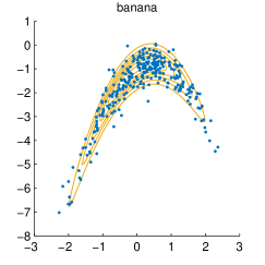
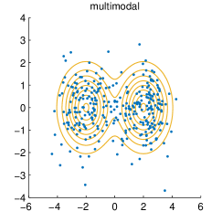
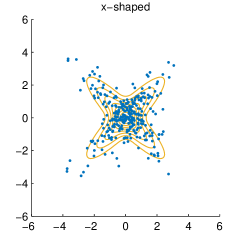
Figure 2: The samples from the variational distribution fitted with uivi (blue) match the shape of the true synthetic target distributions (orange) considered in Section 4.1.

4.2 Bayesian Multinomial Logistic Regression

We now consider Bayesian multinomial logistic regression. For a dataset of $N$ features $x_{n}$ and labels $y_{n}\in\{1,\ldots,K\}$, the model is $p(z)\prod_{n}p(y_{n}\,|\,x_{n},z)$, where $z$ denotes the latent weights and biases. We set the prior $p(z)$ to be Gaussian with identity covariance and zero mean; the categorical likelihood is $p(y_{n}=k\,|\,x_{n},z)\propto\exp(x_{n}^{\top}z_{k}+z_{0k})$.

Datasets.  We use two datasets, mnist and hapt, both available online. mnist contains $60{,}000$ training and $10{,}000$ test instances of $28\times 28$ images of hand-written digits; thus there are $K=10$ classes. We divide pixel values by $255$ so that each feature is bounded between $0$ and $1$. hapt (Reyes-Ortiz et al., 2016) is a human activity recognition dataset. It contains $7{,}767$ training and $3{,}162$ test $561$-dimensional measurements captured by the sensors on a smartphone. There are $K=12$ activities, including static postures (e.g., standing), dynamic activities (e.g., walking), and postural transitions (e.g., stand-to-sit).

Variational family.  We use the variational family described in Section 4.1, namely, a Gaussian prior $q(\varepsilon)$ and Gaussian conditional $q_{\theta}(z\,|\,\varepsilon)$ with diagonal covariance. We set the dimensionality of $\varepsilon$ to $100$, and we use $200$ hidden units on each of the two hidden layers of the neural network that parameterizes the mean of the Gaussian conditional.

Experimental setup.  We run $100{,}000$ iterations of uivi, with the same experimental setup described in Section 4.1. To speed up the procedure, we subsample minibatches of data at each iteration of the algorithm (Hoffman et al., 2013). We use a minibatch size of $2{,}000$ for mnist and $863$ for hapt. For the comparison with sivi, we set the parameter $L=200$ in Eq. 11. We use the same initialization of the variational parameters for both sivi and uivi.

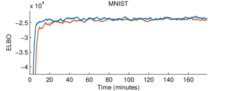
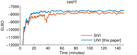
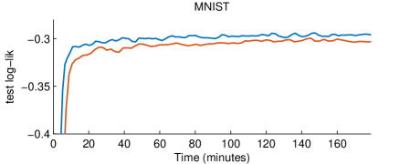
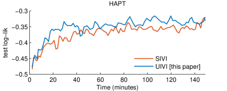
Figure 3: Estimates of the elbo and the test log-likelihood as a function of wall-clock time for the Bayesian multinomial logistic regression model (Section 4.2). Compared to sivi (red), uivi (blue) achieves a better bound on the marginal likelihood and has better predictive performance.

Results.  We found that the time per iteration was comparable for both methods. On average, sivi took $0.14$ seconds per iteration on mnist and $0.09$ seconds on hapt, while uivi took $0.11$ and $0.10$ seconds, respectively.

We obtain a Monte Carlo estimate of the evidence lower bound (elbo) every $100$ iterations (we use $100$ samples, and we use $10{,}000$ samples from $q(\varepsilon)$ to approximate the intractable entropy term). Figure 3 (top) shows the elbo estimates; the plot has been smoothed using a rolling window of size $20$ for easier visualization. uivi provides a similar bound on the marginal likelihood than sivi on mnist and a slightly tighter bound on hapt.

In addition, we also estimate the predictive log-likelihood on the test set every $1{,}000$ iterations (we use $8{,}000$ samples from the variational distribution to form this estimator). Figure 3 (bottom) shows the test log-likelihood as a function of the wall-clock time for both methods and datasets; the plot has been smoothed with a rolling window of size $2$. uivi achieves better predictions on both datasets.

Finally, we study the impact of the number of hmc iterations on the results. In Figure 4, we plot the elbo as a function of the iterations of the variational algorithm in four different settings on the mnist dataset. Each of these settings corresponds to a different number of hmc iterations for both burn-in and sampling periods, ranging from $1$ to $50$ iterations (the standard setting of Figure 3 corresponds to $5$ iterations). We conclude that the number of hmc iterations does not have a significant impact on the results. (Although not included here, the plot for the test log-likelihood shows no significant differences either.)

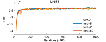
Figure 4: Estimates of the elbo for the Bayesian multinomial logistic regression model (Section 4.2), obtained with uivi under four different settings, which differ only in the number of hmc iterations. The number of hmc iterations in uivi has a small impact on the results.

4.3 Variational Autoencoders

The vae (Kingma & Welling, 2014) defines a conditional likelihood $p_{\phi}(x_{n}\,|\,z_{n})$ given the latent variable $z_{n}$, parameterized by a neural network with parameters $\phi$. The goal is to learn the parameters $\phi$, for which the vae introduces an amortized variational distribution $q_{\theta}(z_{n}\,|\,x_{n})$. In the standard vae, the variational distribution is Gaussian; we use instead a semi-implicit variational distribution.

Datasets.  We use two datasets: (i) the binarized mnist data (Salakhutdinov & Murray, 2008), which contains $50{,}000$ training images and $10{,}000$ test images of handwritten digits; and (ii) the binarized Fashion-mnist data (Xiao et al., 2017), which contains $60{,}000$ training images and $10{,}000$ test images of clothing items. We binarize the Fashion-mnist images with a threshold at $0.5$. Images in both datasets are of size $28\times 28$ pixels.

Variational family.  We use the variational family described in Section 4.1 with Gaussian prior and Gaussian conditional. Since the variational distribution is amortized, we let the conditional $q_{\theta}(z_{n}\,|\,\varepsilon_{n},x_{n})$ depend on the observation $x_{n}$, such that the variational distribution is $q_{\theta}(z_{n}\,|\,x_{n})=\int q(\varepsilon_{n})q_{\theta}(z_{n}\,|\,\varepsilon_{n},x_{n})d\varepsilon_{n}$. We obtain the mean of the Gaussian conditional as the output of a neural network having as inputs both $x_{n}$ and $\varepsilon_{n}$. We set the dimensionality of $\varepsilon_{n}$ to $10$ and the width of each the two hidden layers of the neural network to $200$.

For comparisons, we also fit a standard vae (Kingma & Welling, 2014). The standard vae uses an explicit Gaussian distribution whose mean and covariance are functions of the input, i.e., $q_{\theta}(z_{n}\,|\,x_{n})=\mathcal{N}(z_{n}\,|\,\mu_{\theta}(x_{n}),\Sigma_{\theta}(x_{n}))$. The mean and covariance are parameterized using two separate neural networks with the same structure described above, and the covariance is set to be diagonal. The neural network for the covariance has softplus activations in the output layer, i.e., $\textrm{softplus}(x)=\log(1+e^{x})$.

Experimental setup.  For the generative model $p_{\phi}(x_{n}\,|\,z_{n})$ we use a factorized Bernoulli distribution. We use a two-hidden-layer neural network with $200$ hidden units on each hidden layer, whose sigmoidal outputs define the means of the Bernoulli distribution. We set the prior $p(z_{n})=\mathcal{N}(z_{n}\,|\,0,I)$ and the dimensionality of $z_{n}$ to $10$. We run $400{,}000$ iterations of each method (explicit variational distribution, sivi, and uivi), using the same initialization and a minibatch of size $100$. We set the sivi parameter $L=100$ so that both sivi and uivi have similar complexity (see below). We set the learning rate $\eta=10^{-3}$ for the network parameters of the variational Gaussian conditional, $\eta=2\cdot 10^{-4}$ for its covariance (we also set $\eta=2\cdot 10^{-4}$ for the network that parameterizes the covariance of the explicit distribution), and $\eta=10^{-3}$ for the network parameters of the generative model. We reduce the learning rate by a factor of $0.9$ every $15{,}000$ iterations.

	average test log-likelihood
method	mnist	Fashion-mnist
Explicit (standard vae)	$-98.29$	$-126.73$
sivi	$-97.77$	$-121.53$
uivithis paper	$\mathbf{-94.09}$	$\mathbf{-110.72}$

Table 2: Estimates of the marginal log-likelihood on the test set for the vae (Section 4.3). uivi gives better predictive performance than sivi.

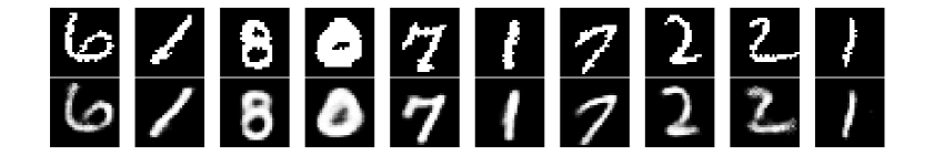
(a) mnist images.

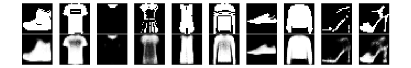
(b) Fashion-mnist images.

Figure 5: Ten images reconstructed with the vae model fitted with uivi (Section 4.3). For each dataset, the top row shows training instances; the bottom row corresponds to the reconstructed images.

Results.  We estimate the marginal likelihood on the test set using importance sampling,

$$\begin{split}&\log p(x_{n})\approx\log\frac{1}{S}\sum_{s=1}^{S}\frac{p_{\phi}(x_{n}\,|\,z_{n}^{(s)})p(z_{n}^{(s)})}{\frac{1}{M}\sum_{m=1}^{M}q_{\theta}(z_{n}^{(s)}\,|\,\varepsilon_{n}^{(m)},x_{n})},\\ &z_{n}^{(s)}\sim q_{\theta}(z_{n}\,|\,x_{n}),\quad\varepsilon_{n}^{(m)}\sim q(\varepsilon),\end{split}$$

where we set $S=1{,}000$ and $M=10{,}000$ samples.

Table 2 shows the estimated values of the test marginal likelihood for all methods and datasets. uivi provides better predictive performance than sivi, which in turn gives better predictions than the explicit Gaussian approximation.

In terms of computational complexity, the average time per iteration is similar for uivi and sivi. On mnist, it is $0.14$ seconds for uivi and $0.16$ seconds for sivi; on Fashion-mnist, it is $0.13$ seconds for uivi and $0.17$ for sivi.

Finally, we show in Figure 5 ten training images from each dataset, together with the corresponding images reconstructed using the vae fitted with uivi. We reconstruct an image by first sampling $z_{n}\sim q_{\theta}(z_{n}\,|\,x_{n})$ and then setting the reconstructed $\hat{x}_{n}$ to the mean given by the generative model $p_{\phi}(x_{n}\,|\,z_{n})$. We conclude that uivi is an effective method to optimize the vae model.

5 CONCLUSION

We have developed unbiased implicit variational inference (uivi), a method to approximate a target distribution with an expressive variational distribution. The variational distribution is implicit, and it is obtained through a reparameterizable distribution whose parameters follow a flexible distribution, similarly to semi-implicit variational inference (sivi) (Yin & Zhou, 2018). In contrast to sivi, uivi directly optimizes the evidence lower bound (elbo) rather than a bound. For that, uivi expresses the gradient of the elbo as an expectation, enabling Monte Carlo estimates of the gradient. Compared to sivi, we show that uivi achieves better elbo and predictive performance for Bayesian multinomial logistic regression and variational autoencoder.

Acknowledgements

Francisco J. R. Ruiz is supported by the EU Horizon 2020 programme (Marie Skłodowska-Curie Individual Fellowship, grant agreement 706760).

References

- Bishop et al. (1998) Bishop, C. M., Lawrence, N. D., Jaakkola, T. S., and Jordan, M. I. Approximating posterior distributions in belief networks using mixtures. In Advances in Neural Information Processing Systems, 1998.
- Blei et al. (2017) Blei, D. M., Kucukelbir, A., and McAuliffe, J. D. Variational inference: A review for statisticians. Journal of the American Statistical Association, 112(518):859–877, 2017.
- Carbonetto et al. (2009) Carbonetto, P., King, M., and Hamze, F. A stochastic approximation method for inference in probabilistic graphical models. In Advances in Neural Information Processing Systems, 2009.
- Dinh et al. (2017) Dinh, L., Sohl-Dickstein, J., and Bengio, S. Density estimation using real NVP. In International Conference on Learning Representations, 2017.
- Figurnov et al. (2018) Figurnov, M., Mohamed, S., and Mnih, A. Implicit reparameterization gradients. In Advances in Neural Information Processing Systems, 2018.
- Gershman et al. (2012) Gershman, S. J., Hoffman, M. D., and Blei, D. M. Nonparametric variational inference. In International Conference on Machine Learning, 2012.
- Ghahramani & Beal (2001) Ghahramani, Z. and Beal, M. J. Propagation algorithms for variational Bayesian learning. In Advances in Neural Information Processing Systems, 2001.
- Ghahramani & Jordan (1997) Ghahramani, Z. and Jordan, M. I. Factorial hidden Markov models. Machine Learning, 29(2–3):245–273, 1997.
- Giordano et al. (2015) Giordano, R. J., Broderick, T., and Jordan, M. I. Linear response methods for accurate covariance estimates from mean field variational Bayes. In Advances in Neural Information Processing Systems, 2015.
- Giordano et al. (2017) Giordano, R. J., Broderick, T., and Jordan, M. I. Covariances, robustness, and variational Bayes. In arXiv:1709.02536, 2017.
- Goodfellow et al. (2014) Goodfellow, I., Pouget-Abadie, J., Mirza, M., Xu, B., Warde-Farley, D., Ozair, S., Courville, A., and Bengio, Y. Generative adversarial nets. In Advances in Neural Information Processing Systems, 2014.
- Grover et al. (2018) Grover, A., Gummadi, R., Lázaro-Gredilla, M., Schuurmans, D., and Ermon, S. Variational rejection sampling. In Artificial Intelligence and Statistics, 2018.
- Guo et al. (2016) Guo, F., Wang, X., Fan, K., Broderick, T., and Dunson, D. B. Boosting variational inference. In arXiv:1611.05559, 2016.
- Han et al. (2016) Han, S., Liao, X., Dunson, D. B., and Carin, L. Variational Gaussian copula inference. In Artificial Intelligence and Statistics, 2016.
- Hoffman et al. (2013) Hoffman, M. D., Blei, D. M., Wang, C., and Paisley, J. Stochastic variational inference. Journal of Machine Learning Research, 14:1303–1347, May 2013.
- Huszár (2017) Huszár, F. Variational inference using implicit distributions. In arXiv:1702.08235, 2017.
- Jaakkola & Jordan (1998) Jaakkola, T. S. and Jordan, M. I. Improving the mean field approximation via the use of mixture distributions. In Learning in Graphical Models, pp. 163–173, 1998.
- Jordan (1999) Jordan, M. I. (ed.). Learning in Graphical Models. MIT Press, Cambridge, MA, USA, 1999.
- Kingma & Welling (2014) Kingma, D. P. and Welling, M. Auto-encoding variational Bayes. In International Conference on Learning Representations, 2014.
- Kingma et al. (2016) Kingma, D. P., Salimans, T., Jozefowicz, R., Chen, X., Sutskever, I., and Welling, M. Improved variational inference with inverse autoregressive flow. In Advances in Neural Information Processing Systems, 2016.
- Kucukelbir et al. (2015) Kucukelbir, A., Ranganath, R., Gelman, A., and Blei, D. M. Automatic variational inference in Stan. In Advances in Neural Information Processing Systems, 2015.
- Kucukelbir et al. (2017) Kucukelbir, A., Tran, D., Ranganath, R., Gelman, A., and Blei, D. M. Automatic differentiation variational inference. Journal of Machine Learning Research, 18(14):1–45, 2017.
- Le et al. (2018) Le, T. A., Igl, M., Rainforth, T., Jin, T., and Wood, F. Auto-encoding sequential Monte-Carlo. In International Conference on Learning Representations, 2018.
- Li & Turner (2018) Li, Y. and Turner, R. E. Gradient estimators for implicit models. In International Conference on Learning Representations, 2018.
- Maaløe et al. (2016) Maaløe, L., Sønderby, C. K., Sønderby, K., and Winther, O. Auxiliary deep generative models. In International Conference on Machine Learning, 2016.
- Maddison et al. (2017) Maddison, C. J., Lawson, D., Tucker, G., Heess, N., Norouzi, M., Mnih, A., Doucet, A., and Teh, Y. W. Filtering variational objectives. In Advances in Neural Information Processing Systems, 2017.
- Mescheder et al. (2017) Mescheder, L., Nowozin, S., and Geiger, A. Adversarial variational Bayes: Unifying variational autoencoders and generative adversarial networks. In International Conference on Machine Learning, 2017.
- Miller et al. (2017) Miller, A. C., Foti, N., and Adams, R. P. Variational boosting: Iteratively refining posterior approximations. In International Conference on Machine Learning, 2017.
- Mohamed & Lakshminarayanan (2016) Mohamed, S. and Lakshminarayanan, B. Learning in implicit generative models. In arXiv:1610.03483, 2016.
- Molchanov et al. (2019) Molchanov, D., Kharitonov, V., Sobolev, A., and Vetrov, D. Doubly semi-implicit variational inference. In Artificial Intelligence and Statistics, 2019.
- Naesseth et al. (2017) Naesseth, C., Ruiz, F. J. R., Linderman, S., and Blei, D. M. Reparameterization gradients through acceptance-rejection methods. In Artificial Intelligence and Statistics, 2017.
- Naesseth et al. (2018) Naesseth, C., Linderman, S. W., Ranganath, R., and Blei, D. M. Variational sequential Monte Carlo. In Artificial Intelligence and Statistics, 2018.
- Neal (2011) Neal, R. M. MCMC using Hamiltonian dynamics. In Brooks, S., Gelman, A., Jones, G. L., and Meng, X.-L. (eds.), Handbook of Markov Chain Monte Carlo. Chapman and Hall/CRC, 2011.
- Nowozin et al. (2016) Nowozin, S., Cseke, B., and Tomioka, R. f-GAN: training generative neural samplers using variational divergence minimization. In Advances in Neural Information Processing Systems, 2016.
- Paisley et al. (2012) Paisley, J. W., Blei, D. M., and Jordan, M. I. Variational Bayesian inference with stochastic search. In International Conference on Machine Learning, 2012.
- Papamakarios et al. (2017) Papamakarios, G., Murray, I., and Pavlakou, T. Masked autoregressive flow for density estimation. In Advances in Neural Information Processing Systems, 2017.
- Ranganath et al. (2014) Ranganath, R., Gerrish, S., and Blei, D. M. Black box variational inference. In Artificial Intelligence and Statistics, 2014.
- Ranganath et al. (2016) Ranganath, R., Tran, D., and Blei, D. M. Hierarchical variational models. In International Conference on Machine Learning, 2016.
- Reyes-Ortiz et al. (2016) Reyes-Ortiz, J. L., Oneto, L., Samà, A., Parra, X., and Anguita, D. Transition-aware human activity recognition using smartphones. Neurocomputing, 171(C):754–767, jan 2016.
- Rezende & Mohamed (2015) Rezende, D. J. and Mohamed, S. Variational inference with normalizing flows. In International Conference on Machine Learning, 2015.
- Rezende et al. (2014) Rezende, D. J., Mohamed, S., and Wierstra, D. Stochastic backpropagation and approximate inference in deep generative models. In International Conference on Machine Learning, 2014.
- Robert & Casella (2005) Robert, C. P. and Casella, G. Monte Carlo Statistical Methods (Springer Texts in Statistics). Springer-Verlag New York, Inc., Secaucus, NJ, USA, 2005.
- Roeder et al. (2017) Roeder, G., Wu, Y., and Duvenaud, D. Sticking the landing: Simple, lower-variance gradient estimators for variational inference. In Advances in Neural Information Processing Systems, 2017.
- Salakhutdinov & Murray (2008) Salakhutdinov, R. and Murray, I. On the quantitative analysis of deep belief networks. In International Conference on Machine Learning, 2008.
- Salimans & Knowles (2013) Salimans, T. and Knowles, D. A. Fixed-form variational posterior approximation through stochastic linear regression. Bayesian Analysis, 8(4):837–882, 2013.
- Salimans et al. (2015) Salimans, T., Kingma, D. P., and Welling, M. Markov chain Monte Carlo and variational inference: Bridging the gap. In International Conference on Machine Learning, 2015.
- Saul & Jordan (1996) Saul, L. K. and Jordan, M. I. Exploiting tractable substructures in intractable networks. In Advances in Neural Information Processing Systems, 1996.
- Shi et al. (2018a) Shi, J., Sun, S., and Zhu, J. Kernel implicit variational inference. In International Conference on Learning Representations, 2018a.
- Shi et al. (2018b) Shi, J., Sun, S., and Zhu, J. A spectral approach to gradient estimation for implicit distributions. In International Conference on Machine Learning, 2018b.
- Sugiyama et al. (2012) Sugiyama, M., Suzuki, T., and Kanamori, T. Density ratio estimation in machine learning. Cambridge University Press, 2012.
- Tieleman & Hinton (2012) Tieleman, T. and Hinton, G. Lecture 6.5-RMSPROP: Divide the gradient by a running average of its recent magnitude. Coursera: Neural Networks for Machine Learning, 4, 2012.
- Titsias & Lázaro-Gredilla (2011) Titsias, M. K. and Lázaro-Gredilla, M. Spike and slab variational inference for multi-task and multiple kernel learning. In Advances in Neural Information Processing Systems, 2011.
- Titsias & Lázaro-Gredilla (2014) Titsias, M. K. and Lázaro-Gredilla, M. Doubly stochastic variational Bayes for non-conjugate inference. In International Conference on Machine Learning, 2014.
- Tomczak & Welling (2016) Tomczak, J. M. and Welling, M. Improving variational auto-encoders using convex combination linear inverse autoregressive flow. In arXiv:1706.02326, 2016.
- Tomczak & Welling (2017) Tomczak, J. M. and Welling, M. Improving variational auto-encoders using Householder flow. In arXiv:1611.09630, 2017.
- Tran et al. (2015) Tran, D., Blei, D. M., and Airoldi, E. M. Copula variational inference. In Advances in Neural Information Processing Systems, 2015.
- Tran et al. (2016) Tran, D., Ranganath, R., and Blei, D. M. Variational Gaussian processes. In International Conference on Learning Representations, 2016.
- Tran et al. (2017) Tran, D., Ranganath, R., and Blei, D. M. Hierarchical implicit models and likelihood-free variational inference. In Advances in Neural Information Processing Systems, 2017.
- Wainwright & Jordan (2008) Wainwright, M. J. and Jordan, M. I. Graphical models, exponential families, and variational inference. Foundations and Trends in Machine Learning, 1(1–2):1–305, January 2008.
- Xiao et al. (2017) Xiao, H., Rasul, K., and Vollgraf, R. Fashion-MNIST: A novel image dataset for benchmarking machine learning algorithms. In arXiv:1708.07747, 2017.
- Yin & Zhou (2018) Yin, M. and Zhou, M. Semi-implicit variational inference. In International Conference on Machine Learning, volume 80 of Proceedings of Machine Learning Research, pp. 5660–5669. PMLR, 2018.
- Zhang et al. (2017) Zhang, C., Bütepage, J., Kjellström, H., and Mandt, S. Advances in variational inference. arXiv:1711.05597, 2017.