Temperature dependence of butterfly effect in a classical many-body system

Abstract

We study the chaotic dynamics in a classical many-body system of interacting spins on the kagome lattice. We characterise many-body chaos via the butterfly effect as captured by an appropriate out-of-time-ordered correlator. Due to the emergence of a spin liquid phase, the chaotic dynamics extends all the way to zero temperature. We thus determine the full temperature dependence of two complementary aspects of the butterfly effect: the Lyapunov exponent, $\mu$, and the butterfly speed, $v_{b}$, and study their interrelations with usual measures of spin dynamics such as the spin-diffusion constant, $D$ and spin-autocorrelation time, $\tau$. We find that they all exhibit power law behaviour at low temperature, consistent with scaling of the form $D\sim v_{b}^{2}/\mu$ and $\tau^{-1}\sim T$. The vanishing of $\mu\sim T^{0.48}$ is parametrically slower than that of the corresponding quantum bound, $\mu\sim T$, raising interesting questions regarding the semi-classical limit of such spin systems.

Introduction: Chaos Dellago and Posch (1997); Hoover et al. (2002); Latora et al. (1998); van Zon et al. (1998); van Beijeren et al. (1997); de Wijn and van Beijeren (2004); de Wijn (2005); de Wijn et al. (2012, 2013); Gaspard et al. (1998, 1999) underpins much of statistical mechanics, providing the basis for ergodicity, thermalization and transport in many-body systems. Perhaps its most striking feature that has captured public imagination is the butterfly effect Lorenz (1963, 1993, 2001); Hilborn (2004): an infinitesimal local change of initial condition is amplified exponentially (Lyapunov exponent $\mu$) and spreads out ballistically (butterfly speed $v_{b}$) to dramatically affect global outcomes.

Quantitative connections between characteristic time and length scales of the chaotic dynamics of a many-body system and those related to its thermalization and transport are far from settled, receiving renewed attention particularly for quantum many-body systems Maldacena et al. (2016); Hosur et al. (2016); Roberts et al. (2015); Roberts and Stanford (2015); Shenker and Stanford (2014); Cotler et al. (2017); Dóra and Moessner (2017); Menezes and Marino (2018); Rozenbaum et al. (2017); Luitz and Bar Lev (2017); Kukuljan et al. (2017); Aleiner et al. (2016); Lin and Motrunich (2018); Chen et al. (2016); Chan et al. (2017); Nahum et al. (2018); von Keyserlingk et al. (2018); Rakovszky et al. (2017); Khemani et al. (2017); Stanford (2016); Patel et al. (2017); Chowdhury and Swingle (2017). There, diagnostic tools of chaos akin to $\mu$ and $v_{b}$ were obtained in an appropriately defined limit of out-of-time-ordered commutators (OTOC) Srednicki (1994); Gutzwiller (1991); Larkin and Ovchinnikov (1969). Further, in a recent study of classical spin chain at infinite temperature Das et al. (2018), the classical limit of OTOC’s has been shown to characterize these features of the butterfly effect.

Here, we study the evolution of the chaotic dynamics as a function of temperature, $T$, of the many body system, and its interrelation with thermalization and transport quantities such as relaxation and diffusion. This is interesting as correlations develop due to interactions as $T$ is lowered, thereby affecting the dynamics of the system. Generally, one expects that at low $T$, the effect of chaos may be weakened due to emergence of long-lived quasi-particles (with or without spontaneously broken symmetry) that dominate the dynamics. Indeed, recent studies of the quantum Sachdev-Ye-Kitaev (SYK) Sachdev and Ye (1993); kit ; Banerjee and Altman (2017); Song et al. (2017) and finite density fermions coupled to gauge fields Patel and Sachdev (2017) (both in the large $N$ limit), show that the absence of quasi-particles due to interactions can lead to chaos as manifested in OTOCs even at the lowest $T$.

We explore these issues in an interacting many-body classical spin system with local interactions on a two dimensional kagome lattice. We elucidate the $T$-dependence of Lyapunov exponent and butterfly speed and find connections between diffusion and chaos over the entire temperature range. At low $T$, Lyapunov exponent ($\mu\sim T^{0.48}$) and butterfly speed ($v_{b}\sim T^{0.23}$), extracted from a classical OTOC Das et al. (2018), show novel algebraic scaling with $T$. This behaviour is qualitatively distinct from that of the quantum counterparts since the observed sub-linear scaling of the Lyapunov exponent is at odds with the quantum low-$T$ bound ($\mu\leq 2\pi k_{B}T/\hbar$ Maldacena et al. (2016)). This raises questions regarding the presumably singular nature of semi-classical (in $1/S$ sense) corrections Kurchan (2016); Scaffidi and Altman (2017) in this spin system. However, in spite of the seeming “violation” of the quantum bound, our results are consistent with a recently identified connections of these microscopic measures of chaos and the macroscopic phenomenon of transport, where for the SYK-model and “strange” metals the energy diffusion constant was found to scale as $D\sim v_{b}^{2}/\mu$Gu et al. (2017); Blake (2016); Blake et al. (2017); Werman et al. (2017); Lucas (2017).

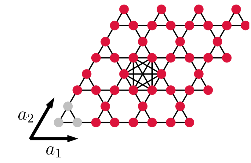
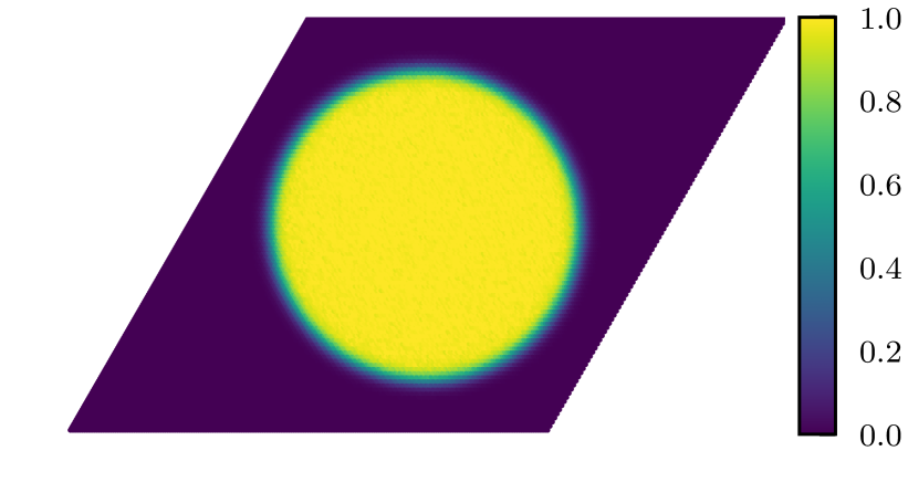
Figure 1: Left: The classical Heisenberg model hosting the $\mathbb{Z}_{2}$ spin liquid is defined on the Kagome lattice with couplings fully connecting all hexagons (only shown for central one). Indicated are the basis vectors $a_{1},a_{2}$ and a possible unit cell (light gray vertices). Right: Snapshot of the dynamics of the de-correlator $D(x,t)$ showing ballistic isotropic spreading of a perturbation initially localised in the centre of the system.

Persistence of chaotic dynamics, usually characteristic to high $T$, in our spin system all the way down to $T=0$ owes its origin to competing (frustrated) local interactions that completely suppresses magnetic ordering.

Model: We study classical $O(3)$ Heisenberg spins of unit length, ${\bf S}_{\bf x}$, on the sites ${\bf x}$ of the kagome lattice,

$$H=J\sum_{{\bf x,x^{\prime}}\in\hexagon}\mathbf{S}_{\bf x}\cdot\mathbf{S}_{\bf x^{\prime}}=\frac{J}{2}\sum_{\alpha}(\mathbf{L}_{\alpha})^{2}+\textrm{const},$$ (1)

where each spin interacts equally with all the spins with which it shares a hexagon, $\hexagon$ Balents et al. (2002), whose total spin is denoted by $\mathbf{L}_{\alpha}=\sum_{\bf{x}\in\hexagon}\mathbf{S}_{\bf{x}}$, schematically illustrated in Fig. 1.

For antiferromagnetic interactions ($J>0$), ground states satisfy the local constraints $\mathbf{L}_{\alpha}=0$ for each hexagon, which leads to a macroscopically degenerate ground state manifold. The system remains in a paramagnetic state all the way down to $T=0$ which has a finite spin correlation length and exhibits fractionalization Rehn et al. (2017). Interestingly, the system does not freeze or fall out of equilibrium in the entire temperature range. Such a phase has been dubbed a classical ‘$\mathbb{Z}_{2}$’ spin-liquid.

The dynamics is that of spins precessing around their local exchange fields, which conserves total energy $E$, magnetization $M$, as well as the spin norm:

$$\frac{d\mathbf{S}_{\bf{x}}(t)}{dt}=-\mathbf{S}_{\bf{x}}(t)\times\sum_{j}J_{\bf{x}\bf{x^{\prime}}}\mathbf{S}_{\bf{x^{\prime}}}(t)\,.$$ (2)

Numerical simulations: These were performed over a range of temperature $T=10^{-3}$ to $T=100$, and linear system size $L=25$ to $L=201$ with $N_{s}=3L^{2}$ spins and periodic boundary conditions. Results shown are for $L=101$ unless indicated otherwise. The spin dynamics is integrated using an eighth-order Runge-Kutta solver with a time-step chosen such that energy/site and magnetisation/site are conserved to better than $\sim 10^{-8}$. Results are averaged over $10^{4}$ initial states sampled from the Boltzmann distribution via Monte-Carlo. Details on the fitting procedure and exemplary raw data fits can be found in the suppl.mat. sup . We measure energy in units of $J=1$, and distances in units of the lattice spacing $a=1$.

Temperature dependence of dynamics: We begin by discussing the two point spin correlator

$$C({\bf x},t)=\langle{\bf S_{x}}(t)\cdot{\bf S_{0}}(0)\rangle\,,$$ (3)

its Fourier-transform, the dynamical structure factor $\mathcal{S}(\mathbf{q},\omega)$, and the auto-correlator $A(t)=\sum_{\bf{x}}\langle{\bf S_{x}}(t)\cdot{\bf S_{x}}(0)\rangle$.

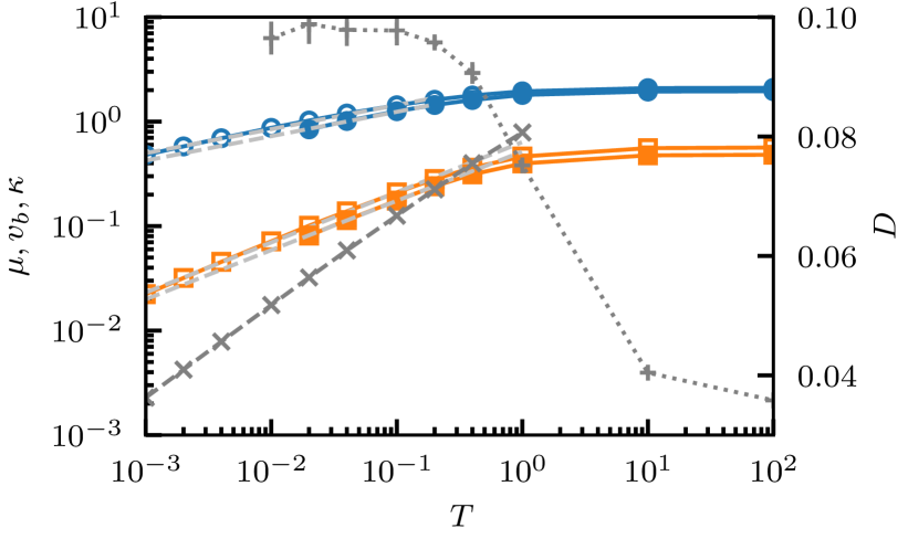
Figure 2: Temperature dependence of various quantities characterising the dynamics and chaos. Relaxation rate $\kappa$ (‘x’) of the auto-correlation function $A(t)\sim e^{-\kappa t}$ on a log-scale (left y-axis) and diffusion constant $D$ (’+’) on a linear scale (right y-axis). Lyapunov exponent $\mu$ (squares) and butterfly velocity $v_{b}$ (circles). Filled symbols results from fits to the scaling form, Eq. 5, empty symbols obtained from independent fits to $D(x=0,t)$ for $\mu$, see Fig. 3, and the arrival times $t_{D_{0}}$ for $v_{b}$, Gray dashed lines are the power-laws fitted to the low-temperature regime. We extract powerlaws $\mu\sim T^{0.48}$ (“ind”), $\mu\sim T^{0.47}$ (“fit”) and $v_{b}\sim T^{0.23}$ in the low-temperature regime respectively.

At all $T$, the autocorrelator exhibits an initial exponential decay $A(t)\sim e^{-\kappa t}$, with diffusion at long wavelengths seen in the tail at long times, $A(t)\sim 1/t$, as well as in the decay of the dynamical structure factor close to the $\Gamma$-point, $\mathcal{S}(\mathbf{q},\omega)\sim 1/[(Dq^{2})^{2}+\omega^{2}]$ sup .

The $T$ dependence of relaxation rate $\kappa$ and diffusion constant $D$ is shown Fig. 2. We observe a linear scaling $\kappa\sim T$, and saturation of the diffusion constant to a constant value, in the low $T$ spin-liquid regime in conformity with the large-$N$ results sup .

Having established and characterised the diffusive behaviour of the spin correlators, we now turn to the main subject of this work, the many-body chaos in this many-body system, in the form of the butterfly effect.

OTOC: We characterise chaos using an analogue of the OTOC in classical spin systems that was constructed in Ref.Das et al. (2018). Considering the evolution of two copies with slightly perturbed initial conditions, we define

$$D(x,t)=1-\langle\mathbf{S}_{x}(t)\cdot\mathbf{\tilde{S}}_{x}(t)\rangle=\langle\left[\delta\mathbf{S}_{x}(t)\right]^{2}\rangle/2$$ (4)

with cross-correlator $\langle\mathbf{S}\cdot\mathbf{\tilde{S}}\rangle$ between copies, the perturbed spin configuration $\mathbf{\tilde{S}}=\mathbf{S}+\delta\mathbf{S}$, and $\langle\cdots\rangle$ an average over the thermodynamic ensemble at $T$.

This de-correlator $D(x,t)$ is expected to scale as

$$D(x,t)\sim\exp[2\mu(1-(v/v_{b})^{\nu})t]$$ (5)

with Lyapunov exponent $\mu$, butterfly velocity $v_{b}$ and an exponent $\nu$, in general all $T$-dependent. The exponent $\nu$ defines the functional form of the velocity-dependent Lyapunov exponent $\lambda(v)=\mu(1-(v/v_{b})^{\nu})$ Kaneko (1986); Deissler (1984); Deissler and Kaneko (1987); Das et al. (2018); Khemani et al. (2018); Xu and Swingle (2018), which measures the exponential growth rate of the de-correlator along rays $v=x/t$. It depends both on the dimensionality, typically decreasing in larger dimensions with decreasing (quantum) fluctuations, and on the presence and type/range of interactions Xu and Swingle (2018); Khemani et al. (2018); Nahum et al. (2018); von Keyserlingk et al. (2018); Lin and Motrunich (2018).

For full quantum models, the Lyapunov exponent inside the light-cone ($v<v_{b}$) has been found to be zero in several examples, whereas in large-N and (semi-)classical models a regime of exponential growth is possible Khemani et al. (2018).

Ballistic Spread of Decorrelation: A snapshot of the decorrelation wavefront at a particular time, as measured by OTOC, is shown in Fig. 1. A light-cone is visible in the dynamics throughout the entire temperature range separating a decorrelated region with $D\sim 1$ centered at the initially perturbed site from a fully correlated unperturbed region with $D\sim 0$. The speed of the ballistally propagating light-cone of the perturbation allows us to define the butterfly speed, $v_{b}$ Lieb and Robinson (1972); Marchioro et al. (1978); Métivier et al. (2014); Roberts and Swingle (2016). The wave-front after an initial transient remains circular over the course of the dynamics and the full temperature range we consider eventhough the underlying lattice only has a six-fold rotational symmetry. This constitutes a non-trivial model-dependent feature of OTOC’s, which generically only need to respect, even at late times, the discrete lattice symmetries Nahum et al. (2018). Thus, it is sufficient to restrict to 1D cuts in the following discussions.

Temperature dependence of $v_{b}$ and $\mu$: The next central result of this study, the full $T$ dependence of Lyapunov exponent $\mu$ and the butterfly velocity $v_{b}$, is shown in Fig. 2. The exponential growth of the decorrelation throughout the entire temperature range confirms the persistence of the chaotic dynamics down to the lowest $T$, in keeping with the persistence of the spin liquid phase.

We employ two methods to extract $\mu$ and $v_{b}$, a fit to the scaling form of the wavefronts, Eq. 5, and independent fits discussed in detail below. Generically, the Lyapunov exponent and butterfly speed extracted from the fit to the full scaling form are slightly lower than those determined independently, which we attribute to subleading prefactors not contained in the scaling form (Eq. 5). Additionally, the independent fits can be extended to lower temperatures than fitting the full wavefront.

For both methods we observe algebraic behaviour at low temperatures: the butterfly speed scales as $\mu\sim T^{0.48\pm 0.006}$ ($T^{0.47\pm 0.005}$) for the independent fit (scaling form) and the Lyapunov exponent as $v_{b}\sim T^{0.23\pm 0.01}$.

The observed scaling of the Lyapunov exponent, $\mu\sim T^{0.48}$, is parametrically larger at low temperatures than the bound on quantum chaos $\mu\leq k_{B}T/h$ Maldacena et al. (2016). While this bound is not directly applicable to our classical model, it implies the semi-classical (say in the form of 1/S) corrections are singular in the low $T$ limit Kurchan (2016); Scaffidi and Altman (2017). At the same time, we note that the observed scaling is consistent with a recently suggested $\sqrt{E}$ behaviour Kurchan (2016).

Interestingly, however, $v_{b}^{2}/\mu$ is approximately constant in the low $T$ regime. This is consistent with the conjectured relation between the diffusion constant $D$, the Lyapunov exponent and butterfly velocity as $D\sim v_{b}^{2}/\mu$ Gu et al. (2017); Blake (2016); Blake et al. (2017); Werman et al. (2017); Lucas (2017), and the fact that we obtain a $T$-independent diffusion constant in the spin-liquid regime (Fig. 2).

We now turn to a detailed discussion of the wavefronts, their ballistic propagation, and scaling form. This also illustrates how the discussed quantities are obtained from the OTOC.

Scaling form:

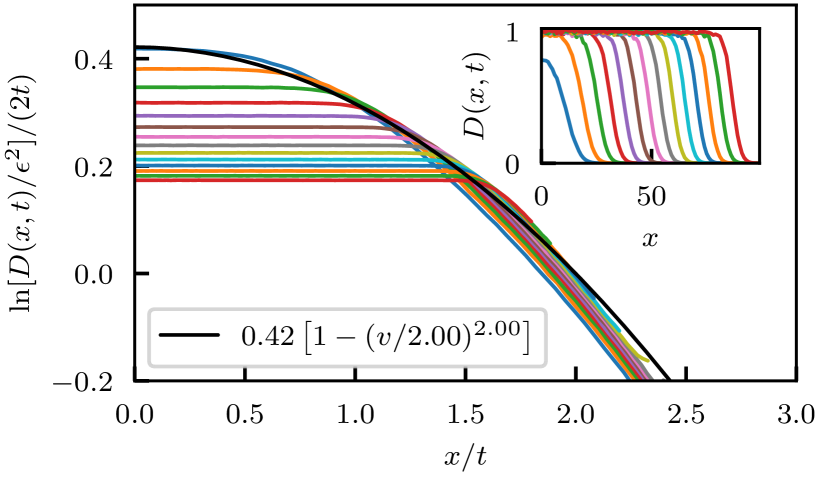
Figure 3: Top: Scaling form and ballistic propagation of the wave-front in the de-correlator $D(x,t)$. The data at the wave-front $v=x/t\sim v_{b}$ well fits Eq. 5 with the parameters given in the box. The inset shows the unscaled data versus distance $x$ at different time-slices $t$ demonstrating the ballistic propagation of the wave-front after an initial growth period. Bottom: De-correlator $D(x=0,t)$ at the initial perturbed site versus time showing exponential growth. Data obtained at $T=100$ on a $L=101$ system, for the non-linear dynamics with $\epsilon=10^{-4}$ and averaged over $10^{4}$ initial states.

Fig. 3 (top panel) shows the scaling form of the de-correlator, according to Eq. 5, and the build-up and propagation of the wavefronts (inset). Close to the wavefront we observe approximate scaling collapse of the de-correlator. In contrast, inside the light-cone we observe deviations from the scaling form due to the saturation of the bounded de-correlators. This is avoided in the linearised version of the dynamics Das et al. (2018), which allows us to directly access the limit of vanishingly small perturbation strength $\epsilon$.

Individual fits: Complementary to fitting the full spatiotemporal profile of $D(x,t)$, which allows access to the velocity dependent Lyapunov exponent $\lambda(v)$, we extract $\mu=\lambda(v=0)$ from an exponential fit to $D(x=0,t)$ and the butterfly velocity $v_{b}$ from the arrival times $t_{D_{0}}(x)$ of the wave-front via $v_{b}=x/t_{D_{0}}$, where $D(x,t_{D_{0}})>D_{0}$ Das et al. (2018).

We demonstrate the expected exponential growth $D(x=0,t)\sim e^{2\mu t}$ in the lower panel of Fig. 3 comparing the linearised dynamics to the non-linear dynamics with $\epsilon=10^{-4}$. In particular, the linearised dynamics shows exponential growth for all times, whereas the linearised dynamics only shows exponential growth over a finite time increasing with smaller perturbation strength as $\log(\epsilon)$ before the decorrelator saturates.

The results for $v_{b}$ and $\mu$ from the non-linear dynamics converge with decreasing perturbation strength $\epsilon$ to the results obtained from the linearised dynamics sup .

We find that the results obtained from the individual fits are generally compatible with the results obtained from fitting to the scaling form. Importantly, it does allow us to reach lower temperatures, where a full wavefront cannot develop on available system sizes before the perturbation reaches the periodic boundaries.

Solitonic wavefronts:

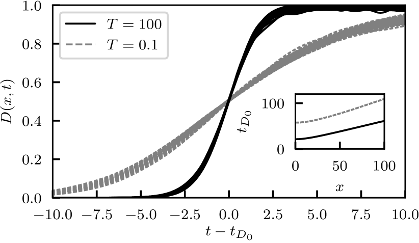
Figure 4: Shape of the propagating wave-front in the de-correlator $D(x,t)$ for temperatures $T=100$ (solid black) and $T=0.1$ (dashed gray). Data at different distances $x$ for $x=10,\cdots,L-10$ are plotted versus time $t$ after collapsing them by subtracting $t_{D_{0}}(x)$ with $D_{0}=0.5$. Inset: Arrival time $t_{D_{0}}$ versus distance $x$ showing linear scaling with distance.

Fig. 4 demonstrates that, like in a soliton, the wavefront shape remains approximately constant as it moves. At least for the times accessible in our simulation, we do not observe significant broadening. Note that here we consider the shape of the full wavefront, rather than the leading edge only, which in principle could show different behaviour due to the non-linearity of the dynamics.

In contrast, we observe strong $T$ dependence of the shape of the wavefront. With decreasing temperatures the front broadens both temporally, Fig. 4, and spatially.

The inset of Fig. 4 shows the linear scaling of the arrival times $t_{D_{0}}(x)$, with distance $x$, and, thus, ballistic propagation of the wavefront. The slowing down of propagation at lower $T$ manifests itself in the larger slope of the arrival times versus distance, whereas the decrease of the Lyapunov exponent with temperature is seen in the larger arrival time $t_{D_{0}}$ at $x=0$.

The observed ballistic dynamics of the de-correlator is in stark contrast to the purely diffusive relaxational dynamics of the spin correlators in the system.

Outlook: We have analysed the $T$-dependence of chaos in a classical many-body system with local interactions, centered around the butterfly effect, with implications for the physics of spin liquids, the classical-quantum correspondence for chaotic spin systems, the relevance of OTOC’s in classical chaos, and the relation of microscopic chaos to macroscopic transport.

Many follow-on questions naturally pose themselves, e.g. concerning the role of phase transitions and order, the nature of the semiclassical limit, and the ‘transition’ into an integrable regime with an increasing number of conserved quantities. Even at the classical level, small perturbations may lead to ordering and a reduction of the dimensionality of the ground state manifold. In such cases the observed effects are expected to survive above the concomitant ordering temperatures, which are often much smaller than the leading interaction scale, opening up a robust spin liquid regime .

Another interesting aspect is the effect of the quantum fluctuations on this classical model. Such quantum fluctuations would, again, generally quench the ground state entropy. However, this may not necessarily lead to an ordered state, but a long range quantum entangled spin liquid state expected for this system in $S=1/2$ limit Balents et al. (2002). The crossover to such a quantum coherent regime would then be accompanied by sharp signature in the indicators of many-body chaos studied above.

Acknowledgements: This work was supported by the Max-Planck partner group on strongly correlated systems at ICTS, the Deutsche Forschungsgemeinschaft under SFB 1143 and SERB-DST (India) through project grant No. ECR/2017/000504. The authors acknowledge fruitful discussion and collaboration on related work with S. Banerjee, A. Dhar, A. Das, D. A. Huse, A. Kundu and S. S. Ray.

Supplemental Material:

I Dynamics of the $\mathbb{Z}_{2}$ spin liquid

I.1 Large-N analytics

The large-N limit relaxes the condition of unit length $O(N)$ spins in the limit of $N\rightarrow\infty$ Garanin and Canals (1999). It reproduces well the static properties of the highly frustrated kagome and pyrochlore Heisenberg models Isakov et al. (2004); Taillefumier et al. (2014). Its extension via a stochastic Langevin dynamics allows accurate predictions also for the dynamics of the classical pyrochlore and kagome models Conlon and Chalker (2009); Taillefumier et al. (2014).

Eventhough the quantitative agreement has been shown to be slightly worse for the $\mathbb{Z}_{2}$ model under consideration here Rehn et al. (2017), it provides an analytically tractable starting point from which to approach the full model dynamics.

Large-N calculation: In the large-N calculation the soft spins follow the (unnormalised) probability distribution $e^{-\beta E}$ with the energy

$$\beta E=\frac{1}{2}\sum_{i}\lambda s_{i}^{2}+\frac{1}{2}\beta J\sum_{\alpha}l_{\alpha}^{2}$$ (S1)

where $l_{\alpha}=\sum_{i\in\alpha}s_{i}$ is the sum of the “soft” spins $s_{i}$ over the hexagon $\alpha$ and $\lambda$ is a lagrange multiplier ensuring the length constraint $\left<s_{i}^{2}\right>=1/3$ (Heisenberg spins).

We may rewrite the interaction term as $\sum_{i,j}s_{i}\left(A_{ij}+2\delta_{ij}\right)s_{j}$ where $A_{ij}$ is the connectivity matrix of the model. We call $M=\left(A_{ij}+2\delta_{ij}\right)$ the interaction matrix.

Since the model is translationally invariant, the eigenbasis is labelled by a momentum $\mathbf{q}$ and a sublattice index $\nu\in\{1,2,3\}$. We obtain two flat bands $\nu_{1,2}(\mathbf{q})=0$ and one dispersive gapped band $\nu_{3}(\vec{q})$.

Dynamics is introduced via the Langevin equation

$$\frac{ds_{i}(t)}{dt}=\Gamma\sum_{l}\left(A_{il}-z\delta_{il}\right)\frac{\partial E}{\partial s_{l}}+\zeta_{i}(t)$$ (S2)

with the coordination number $z$ ($z=10$ in this model), a noise term $\zeta_{i}(t)$ and a free constant $\Gamma$ determining the overall timescale of dynamical processes.

Solving this equation in the eigenbasis $\tilde{s}(\mathbf{q})$ of the interaction matrix $M$ we obtain

$$\left<\tilde{s}^{\mu}_{\mathbf{q}}(t)\tilde{s}^{\nu}_{-\mathbf{q}}(0)\right>=\frac{\delta_{\mu,\nu}T}{Jv_{\mu}+\lambda T}e^{-\Gamma\left(12-v_{\mu}\right)\left(Jv_{\mu}+\lambda T\right)t}$$ (S3)

with a characteristic decay rate $\kappa_{\mu}=\Gamma\left(12-v_{\mu}\right)\left(Jv_{\mu}+\lambda T\right)$.

The dynamical structure factor is given by

$$S(\mathbf{q},t) =\sum_{\nu\mu}\left<s^{\mu}_{\mathbf{q}}(t)s^{\nu}_{-\mathbf{q}}(0)\right>$$ (S4)

$$=\sum_{\alpha}\left(\sum_{\mu\nu}U^{\mu\alpha}_{\mathbf{q}}U^{\nu\alpha}_{-\mathbf{q}}\right)\left<\tilde{s}^{\alpha}_{\mathbf{q}}(t)\tilde{s}^{\alpha}_{-\mathbf{q}}(0)\right>$$ (S5)

$$=\sum_{\alpha}g^{\alpha}_{\mathbf{q}}\left<\tilde{s}^{\alpha}_{\mathbf{q}}(t)\tilde{s}^{\alpha}_{-\mathbf{q}}(0)\right>$$ (S6)

with the factors $g^{\alpha}_{\mathbf{q}}$ defined via the matrix of eigenvectors $U^{\mu\nu}_{\mathbf{q}}$. These factors satisfy the sum rule $\sum_{\alpha}g^{\alpha}=3$.

Autocorrelation: The autocorrelation function shows exponential decay $A(t)=e^{-\kappa t}$ in the low-temperature limit with $\kappa=12\Gamma\lambda T$, i.e. a linear dependence on temperature.

Structure factor: In the low-temperature limit the dynamical structure factor at generic wave-vector is exponentially decaying with a $\mathbf{q}$-independent decay rate scaling with $T$, $\kappa(\mathbf{q})=12\Gamma\lambda T$.

Around $\mathbf{q}=0$ the full weight is in the dispersive band, and we can extract a diffusion constant from $\kappa(\mathbf{q})=Dq^{2}$ with $D=9\,\Gamma J$, i.e. a temperature independent diffusion constant.

II Numerics

II.1 Structure factor

We consider the dynamical structure factor $S(\mathbf{q},t)=\sum_{ij}e^{i\mathbf{q}\cdot(\mathbf{r}_{i}-\mathbf{r}_{j})}\langle\mathbf{S}_{i}(t)\cdot\mathbf{S}_{j}(0)\rangle$ and its fourier transform $S(\mathbf{q},\omega)$ which provides spatially and frequency resolved information on the dynamics.

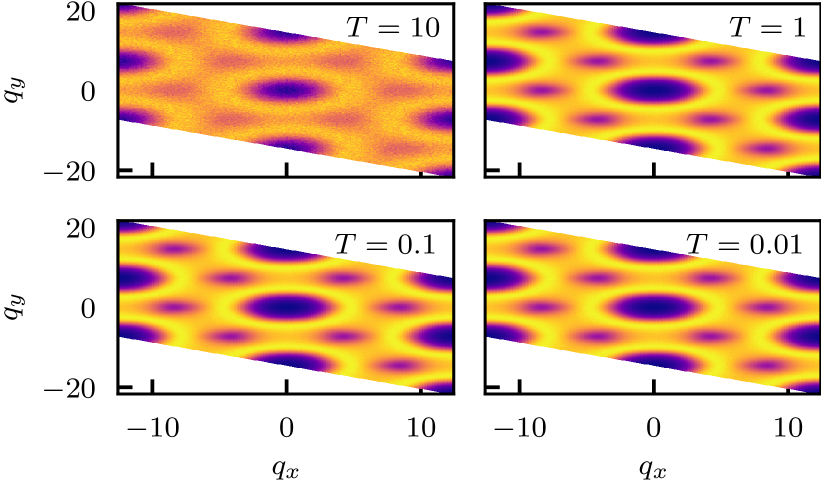
Figure S1: Static structure factor $S(\mathbf{q},t=0)$ for temperatures $T=10$ down to $T=0.01$ as indicated in the figure.

Static structure factor: The static structure factor $S(\mathbf{q},t=0)$ in Fig. S1 for temperatures $T=0.01,0.1,1,10$ shows the transition from the high-temperature paramagnet to the spin liquid regime at low temperatures.

The static structure factor remains essentially unchanged below $T\sim 0.1-1$. In particular, it shows no pinch points or lines and no sign of ordering. The results in the spin-liquid regime are in good agreement with the predictions of the large-N calculations (not shown).

Dynamical structure factor: Since the dynamics, Eq. 2, conserves the total magnetisation, we expect diffusion to occur at small wavevectors.

To test this expectation we perform a scaling collapse of the dynamical structure factor via

$$\beta q^{2}S(\mathbf{q},\omega)\sim\frac{D}{(\omega/q^{2})^{2}+D^{2}}$$ (S7)

appropriate diffusion in 2D. We find an approximate scaling collapse of this form in Fig. S2.

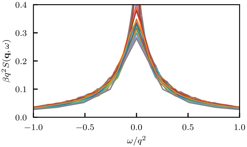
Figure S2: Scaling collapse of the dynamical structure factor $S(\mathbf{q},\omega)$ for $\mathbf{q}$ around the $\Gamma$-point and temperatures $T=0.01,0.02,0.04,0.1$.

To extract the diffusion constant we fit the dynamic structure factor via $S(\mathbf{q},\omega)\sim 1/(\omega^{2}+\kappa(\mathbf{q})^{2})$, corresponding to an exponentially decaying dynamical structure factor with decay rate $\kappa(\mathbf{q})$, i.e. $S(\mathbf{q},t)\sim e^{-\kappa(\mathbf{q})t}$. For diffusive behaviour we expect $\kappa(\mathbf{q})=Dq^{2}$ for momenta $q$ close to the $\Gamma$-point.

Fig. S3 presents the results for $\kappa(q)$ and the quadratic fits to extract the diffusion constant $D$. Already on the level of the raw data we observe a clear separation into the high-temperature paramagnetic phase $T>1$ and the low-temperature spin-liquid regime $T<0.1$.

We also note that with decreasing temperature the range of validity of the quadratic fit shrinks which limits the extraction of the diffusion constant to temperatures $T\geq 0.002$ on the available system sizes, and results in increasing uncertainties at lower temperatures.

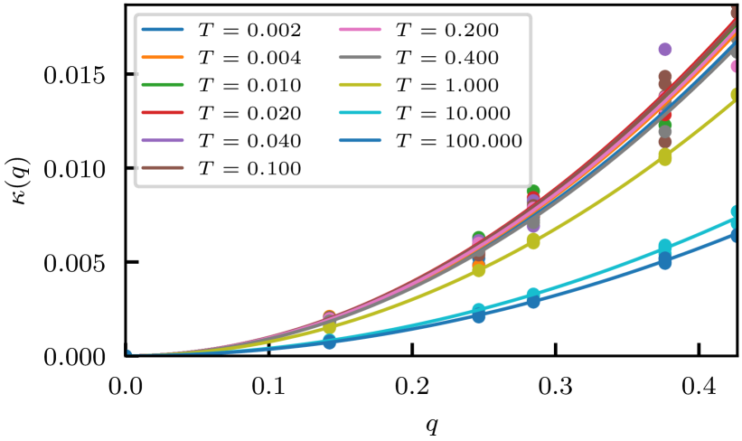
Figure S3: Extraction of the diffusion constant from the dynamical structure. Fits to $\kappa(q)=Dq^{2}$ for a range of temperatures $T=0.002$ up to $T=100$. The data separates into the high temperature regime $T>1$ and the low temperature spin-liquid regime $T<0.1$.

III Butterfly effect in the $\mathbb{Z}_{2}$ spin liquid

III.1 Fitting the full propagating wavefront

As stated in the main text the de-correlator $D(x,t)$ is fit well by the scaling form

$$D(x,t)\sim\exp[2\mu(1-(v/v_{b})^{\nu})t]$$ (S8)

with the Lyapunov exponent $\mu$, the butterfly velocity $v_{b}$ and an exponent $\nu$, which will all generically be temperature dependent.

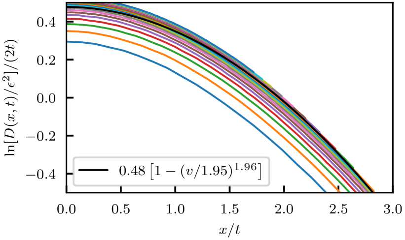
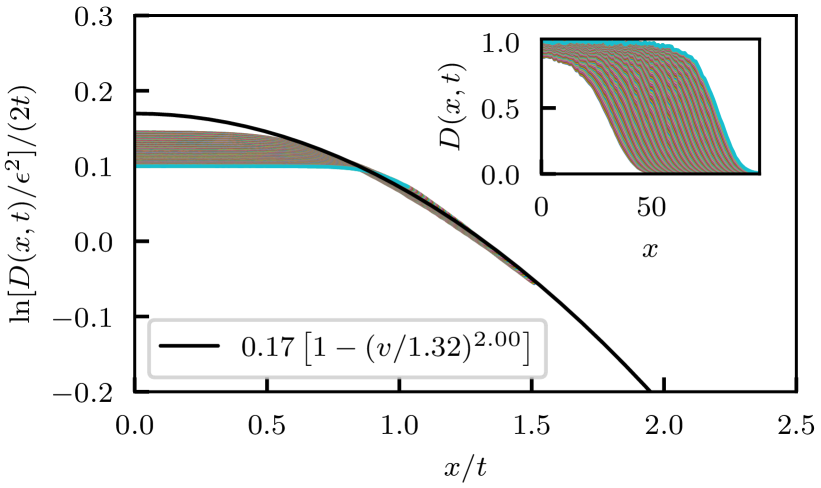
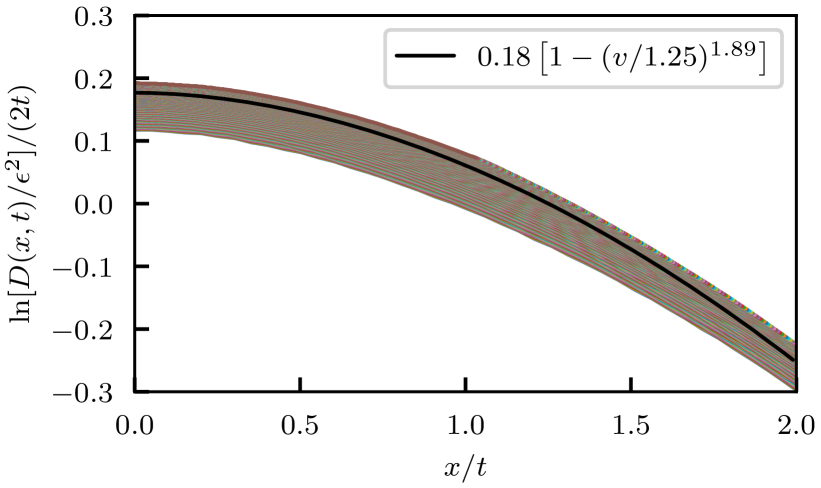
Figure S4: Scaling form and ballistic propagation of wave-fronts in the de-correlator $D(x,t)$. Non-linear dynamics with $\epsilon=10^{-4}$ (left) versus linearised dynamics (right) and $T=100$ (top) versus $T=0.1$ (bottom). The data at the wave-front $v=x/t\sim v_{b}$ well fits Eq. S8 with the parameters given in the box. The inset shows the unscaled data versus distance $x$ at different time-slices $t$ demonstrating the ballistic propagation of the wave-front after an initial growth period.

In Fig. S4 we show typical fits of the scaling form to the results of the de-correlator $D(x,t)$ for the non-linear (left row) and linearised dynamics (right row) for temperatures $T=100$ (top) and $T=0.1$ (bottom).

The non-linear data shows saturation effects inside the light-cone for $v<v_{b}$ when the decorrelation reaches $D\sim 1$. Thus, it only fits the scaling form around $v\sim v_{b}$ and the estimate for $\mu$ is biased to smaller values. The linearised dynamics shows no saturation effects, and therefore provides considerably less spread around the scaling form. Moreover, the remaining spread is further reduced when performing the simulations on larger system sizes.

Smaller temperatures inherently require larger systems for a wave front to build up since the perturbation propagates relatively faster than it grows, thus, reaching the boundaries of the system before it saturates at the initial site. This limits the temperature range we can reliably perform fits to the full wavefronts to $T>0.02$ on systems up to $L=101$.

The linearised dynamics show an extracted exponent $\nu=2$ at $T=100$, which then decreases slightly to $\nu\sim 1.9$ at $T=0.1$. The non-linear dynamics are consistent with a constant exponent $\nu=2$ over the full temperature range considered, however, can also be fit with the exponent extracted from the linearised dynamics.

III.2 Convergence with $\epsilon$

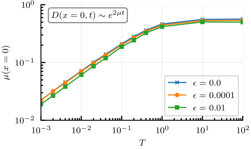
Figure S5: Lyapunov Exponent $\mu$ versus temperature $T$ on a log-log scale, extracted from an exponential fit to the de-correlator at $x=0$ via $D(x=0,t)\sim\exp[2\mu t]$ for the non-linear dynamics with $\epsilon=10^{-4},10^{-2}$ and the linearised dynamics $\epsilon=0$.

Fitting the behaviour of $D(x=0,t)$ via $D(x=0,t)\sim e^{2\mu t}$ allows to extract the (leading) Lyapunov exponent $\mu$. The extracted Lyapunov exponent is shown in Fig. S5 versus temperature. We observe convergence of the extracted Lyapunov exponent with decreasing $\epsilon$ towards the results of the linearised equations across the whole temperature range. We note that this is important for two reasons. Firstly, it shows that our results for $\epsilon=10^{-4}$ are already quite close to the limit of vanishing perturbation strength. Secondly, it implies that the linearised dynamics indeed correctly captures the behaviour of the decorrelator also for finite, but small perturbation strengths.

We may determine the butterfly-speed from the propagation of the wavefront: We define the arrival time $t_{D_{0}}(x)$ at distance $x$ at which the de-correlator $D(x,t)$ exceeds a given threshold $D_{0}$. For ballistic propagation we expect a linear relation with $x=v_{b}\,t_{D_{0}}$.

For sufficiently small thresholds $D_{0}\sim\epsilon^{2}$ we observe the expected linear behaviour of the arrival times with distance $t_{D_{0}}=x/v_{b}$, at least for sites $x$ sufficiently removed from the initially perturbed site. Moreover, choosing $D_{0}=\epsilon^{2}$ we obtain results for the butterfly speed $v_{b}$ independent of the chosen perturbation strength, for sufficiently small $\epsilon$, and in agreement with the linearised dynamics as shown in Fig. S6.

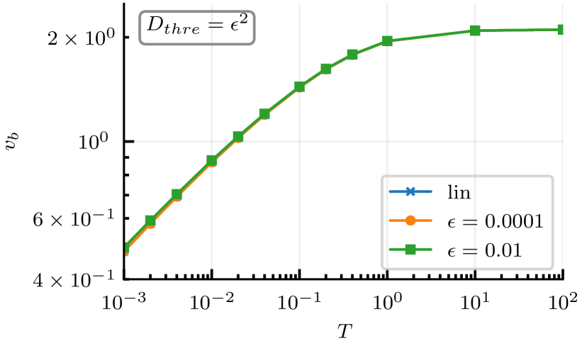
Figure S6: Butterfly speed $v_{b}$ versus temperature $T$ on a log-log scale, extracted from a linear fit to the arrival times $x=v_{b}t_{D_{0}}$ defined via $D(x,t_{D_{0}})>D_{0}$.

III.3 Variation over initial states

In this section we consider the dependence of the extracted quantities on the initial states keeping information for all $10^{4}$ simulated states, but restricting to smaller sizes of $L=51$.

The sample-to-sample variation allows us to determine whether the mean characterises the full state-manifold or whether states at a given temperature might behave differently.

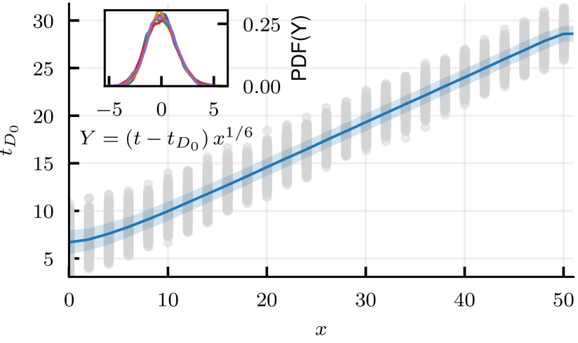
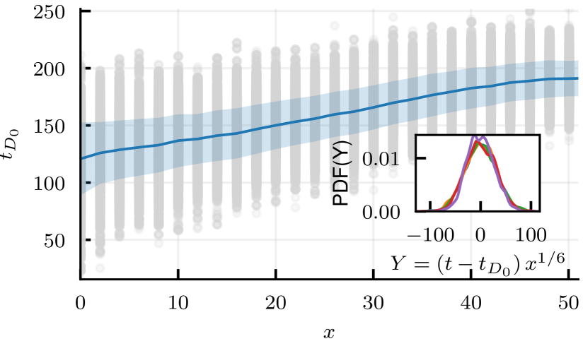
Figure S7: Arrival times $t_{D_{0}}$ as a function of x for $D_{0}=10\epsilon^{2}$ and $\epsilon=10^{-4}$ for temperatures $T=100$ (left) and $T=0.001$ (right). Gray scatter is the variation over different initial spin-configuration, solid blue line the mean value, and the blue shading the standard deviation of the data. The inset shows the distribution of $t_{D_{0}}$ at $x=5,10,15,20,25$ with an approximate collapse on scaling with $x^{1/6}$. Results obtained on a $L=51$ system.

We first consider the variation of the arrival times $t_{D_{0}}$ in Fig. S7. The relation of $t_{D_{0}}$ is linear for all samples apart from boundary effects, either at the initial perturbed site or at half the system size when periodic boundary conditions affect the results.

We observe some scatter in the arrival times, increasing considerably at lower temperature. However, the variance of the arrival times actually appears to decrease with increasing distance $x$ from the perturbed site, or equivalently with time. This is confirmed in the inset by the scaling collapse of the data for $t_{D_{0}}$ with $x^{1/6}$.

However, we emphasise that this might only be true for the accessible times, and this initial decrease could be a transient effect, after which the asymptotic long-time limit could show different behaviour.

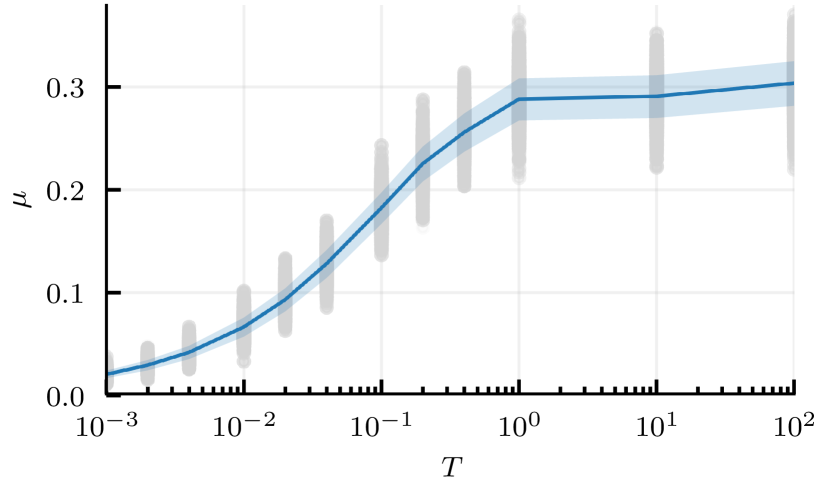
Figure S8: Lyapunov exponent $\mu$ versus temperature $T$, extracted from an exponential fit to the de-correlator at $x=0$ via $D(x=0,t)\sim\exp[2\mu t]$ for different initial states. Gray scatter is the variation over initial states, the solid line the mean, and the blue shading marks the standard deviation of the data. Results obtained for the non-linear dynamics with $\epsilon=10^{-4}$ on a $L=51$ system.

Next, we consider the extraction of the Lyapunov exponent from the de-correlator at $x=0$ via $D(x=0,t)\sim\exp[2\mu t]$. In Fig. S8 we show the variation of $\mu$ at different temperatures $T$ when performing this fit for different initial states individually instead of on the mean of the data. The distribution of $\mu$ over initial states is approximately gaussian at all temperatures and well characterised by its mean and variance, both decreasing with decreasing temperatures.

We note that the average of the extracted Lyapunov exponents over initial states differs from the Lyapunov exponent extracted from the averaged data, since the former is essentially the average of a logarithm, whereas the later is the logarithm of the average.

References

- Dellago and Posch (1997) C. Dellago and H. Posch, “Kolmogorov-Sinai entropy and Lyapunov spectra of a hard-sphere gas,” Physica A: Statistical Mechanics and its Applications 240, 68–83 (1997).
- Hoover et al. (2002) W. G. Hoover, H. A. Posch, C. Forster, C. Dellago, and M. Zhou, “Lyapunov Modes of Two-Dimensional Many-Body Systems; Soft Disks, Hard Disks, and Rotors,” Journal of Statistical Physics 109, 765–776 (2002).
- Latora et al. (1998) V. Latora, A. Rapisarda, and S. Ruffo, “Lyapunov Instability and Finite Size Effects in a System with Long-Range Forces,” Phys. Rev. Lett. 80, 692–695 (1998).
- van Zon et al. (1998) R. van Zon, H. van Beijeren, and C. Dellago, “Largest Lyapunov Exponent for Many Particle Systems at Low Densities,” Phys. Rev. Lett. 80, 2035–2038 (1998).
- van Beijeren et al. (1997) H. van Beijeren, J. R. Dorfman, H. A. Posch, and C. Dellago, “Kolmogorov-Sinai entropy for dilute gases in equilibrium,” Phys. Rev. E 56, 5272–5277 (1997).
- de Wijn and van Beijeren (2004) A. S. de Wijn and H. van Beijeren, “Goldstone modes in Lyapunov spectra of hard sphere systems,” Phys. Rev. E 70, 016207 (2004).
- de Wijn (2005) A. S. de Wijn, “Lyapunov spectra of billiards with cylindrical scatterers: Comparison with many-particle systems,” Phys. Rev. E 72, 026216 (2005).
- de Wijn et al. (2012) A. S. de Wijn, B. Hess, and B. V. Fine, “Largest Lyapunov Exponents for Lattices of Interacting Classical Spins,” Phys. Rev. Lett. 109, 034101 (2012).
- de Wijn et al. (2013) A. S. de Wijn, B. Hess, and B. V. Fine, “Lyapunov instabilities in lattices of interacting classical spins at infinite temperature,” Journal of Physics A: Mathematical and Theoretical 46, 254012 (2013).
- Gaspard et al. (1998) P. Gaspard, M. E. Briggs, M. K. Francis, J. V. Sengers, R. W. Gammon, J. R. Dorfman, and R. V. Calabrese, “Experimental evidence for microscopic chaos,” Nature 394, 865–868 (1998).
- Gaspard et al. (1999) P. Gaspard, M. E. Briggs, M. K. Francis, J. V. Sengers, R. W. Gammon, J. R. Dorfman, and R. V. Calabrese, “Microscopic chaos from brownian motion?” Nature 401, 876–876 (1999).
- Lorenz (1963) E. N. Lorenz, “Deterministic nonperiodic flow,” Journal of the atmospheric sciences 20, 130–141 (1963).
- Lorenz (1993) E. N. Lorenz, The essence of chaos (University of Washington Press, Seattle, Washington, 1993).
- Lorenz (2001) E. Lorenz, “The butterfly effect,” in The Chaos Avant-Garde (World Scientific, 2001) pp. 91–94.
- Hilborn (2004) R. C. Hilborn, “Sea gulls, butterflies, and grasshoppers: A brief history of the butterfly effect in nonlinear dynamics,” American Journal of Physics 72, 425–427 (2004).
- Maldacena et al. (2016) J. Maldacena, S. H. Shenker, and D. Stanford, “A bound on chaos,” Journal of High Energy Physics 2016, 106 (2016).
- Hosur et al. (2016) P. Hosur, X.-L. Qi, D. A. Roberts, and B. Yoshida, “Chaos in quantum channels,” Journal of High Energy Physics 2016, 4 (2016).
- Roberts et al. (2015) D. A. Roberts, D. Stanford, and L. Susskind, “Localized shocks,” Journal of High Energy Physics 2015, 51 (2015).
- Roberts and Stanford (2015) D. A. Roberts and D. Stanford, “Diagnosing Chaos Using Four-Point Functions in Two-Dimensional Conformal Field Theory,” Phys. Rev. Lett. 115, 131603 (2015).
- Shenker and Stanford (2014) S. H. Shenker and D. Stanford, “Black holes and the butterfly effect,” Journal of High Energy Physics 2014, 67 (2014).
- Cotler et al. (2017) J. S. Cotler, G. Gur-Ari, M. Hanada, J. Polchinski, P. Saad, S. H. Shenker, D. Stanford, A. Streicher, and M. Tezuka, “Black holes and random matrices,” Journal of High Energy Physics 2017, 118 (2017).
- Dóra and Moessner (2017) B. Dóra and R. Moessner, “Out-of-Time-Ordered Density Correlators in Luttinger Liquids,” Phys. Rev. Lett. 119, 026802 (2017).
- Menezes and Marino (2018) G. Menezes and J. Marino, “Slow scrambling in sonic black holes,” EPL (Europhysics Letters) 121, 60002 (2018).
- Rozenbaum et al. (2017) E. B. Rozenbaum, S. Ganeshan, and V. Galitski, “Lyapunov Exponent and Out-of-Time-Ordered Correlator’s Growth Rate in a Chaotic System,” Phys. Rev. Lett. 118, 086801 (2017).
- Luitz and Bar Lev (2017) D. J. Luitz and Y. Bar Lev, “Information propagation in isolated quantum systems,” Phys. Rev. B 96, 020406 (2017).
- Kukuljan et al. (2017) I. Kukuljan, S. c. v. Grozdanov, and T. c. v. Prosen, “Weak quantum chaos,” Phys. Rev. B 96, 060301 (2017).
- Aleiner et al. (2016) I. L. Aleiner, L. Faoro, and L. B. Ioffe, “Microscopic model of quantum butterfly effect: Out-of-time-order correlators and traveling combustion waves,” Annals of Physics 375, 378–406 (2016).
- Lin and Motrunich (2018) C.-J. Lin and O. I. Motrunich, “Out-of-time-ordered correlators in a quantum Ising chain,” Phys. Rev. B 97, 144304 (2018).
- Chen et al. (2016) X. Chen, T. Zhou, D. A. Huse, and E. Fradkin, “Out-of-time-order correlations in many-body localized and thermal phases,” Annalen der Physik 529, 1600332 (2016).
- Chan et al. (2017) A. Chan, A. De Luca, and J. T. Chalker, “Solution of a minimal model for many-body quantum chaos,” ArXiv e-prints (2017), arXiv:1712.06836 [cond-mat.stat-mech] .
- Nahum et al. (2018) A. Nahum, S. Vijay, and J. Haah, “Operator Spreading in Random Unitary Circuits,” Phys. Rev. X 8, 021014 (2018).
- von Keyserlingk et al. (2018) C. W. von Keyserlingk, T. Rakovszky, F. Pollmann, and S. L. Sondhi, “Operator Hydrodynamics, OTOCs, and Entanglement Growth in Systems without Conservation Laws,” Phys. Rev. X 8, 021013 (2018).
- Rakovszky et al. (2017) T. Rakovszky, F. Pollmann, and C. W. von Keyserlingk, “Diffusive hydrodynamics of out-of-time-ordered correlators with charge conservation,” ArXiv e-prints (2017), arXiv:1710.09827 [cond-mat.stat-mech] .
- Khemani et al. (2017) V. Khemani, A. Vishwanath, and D. A. Huse, “Operator spreading and the emergence of dissipation in unitary dynamics with conservation laws,” ArXiv e-prints (2017), arXiv:1710.09835 [cond-mat.stat-mech] .
- Stanford (2016) D. Stanford, “Many-body chaos at weak coupling,” Journal of High Energy Physics 2016, 9 (2016).
- Patel et al. (2017) A. A. Patel, D. Chowdhury, S. Sachdev, and B. Swingle, “Quantum Butterfly Effect in Weakly Interacting Diffusive Metals,” Phys. Rev. X 7, 031047 (2017).
- Chowdhury and Swingle (2017) D. Chowdhury and B. Swingle, “Onset of many-body chaos in the model,” Phys. Rev. D 96, 065005 (2017).
- Srednicki (1994) M. Srednicki, “Chaos and quantum thermalization,” Phys. Rev. E 50, 888–901 (1994).
- Gutzwiller (1991) M. C. Gutzwiller, Chaos in Classical and Quantum Mechanics, Interdisciplinary Applied Mathematics (Springer New York, 1991).
- Larkin and Ovchinnikov (1969) A. I. Larkin and Y. N. Ovchinnikov, “Quasiclassical Method in the Theory of Superconductivity,” Soviet Journal of Experimental and Theoretical Physics 28, 1200 (1969).
- Das et al. (2018) A. Das, S. Chakrabarty, A. Dhar, A. Kundu, D. A. Huse, R. Moessner, S. S. Ray, and S. Bhattacharjee, “Light-Cone Spreading of Perturbations and the Butterfly Effect in a Classical Spin Chain,” Phys. Rev. Lett. 121, 024101 (2018).
- Sachdev and Ye (1993) S. Sachdev and J. Ye, “Gapless spin-fluid ground state in a random quantum Heisenberg magnet,” Phys. Rev. Lett. 70, 3339–3342 (1993).
- (43) A. Y. Kitaev, KITP Program: Entanglement in Strongly- Correlated Quantum Matter (2015).
- Banerjee and Altman (2017) S. Banerjee and E. Altman, “Solvable model for a dynamical quantum phase transition from fast to slow scrambling,” Phys. Rev. B 95, 134302 (2017).
- Song et al. (2017) X.-Y. Song, C.-M. Jian, and L. Balents, “Strongly Correlated Metal Built from Sachdev-Ye-Kitaev Models,” Phys. Rev. Lett. 119, 216601 (2017).
- Patel and Sachdev (2017) A. A. Patel and S. Sachdev, “Quantum chaos on a critical Fermi surface,” Proceedings of the National Academy of Sciences 114, 1844–1849 (2017), http://www.pnas.org/content/114/8/1844.full.pdf .
- Kurchan (2016) J. Kurchan, “Quantum bound to chaos and the semiclassical limit,” ArXiv e-prints (2016), arXiv:1612.01278 [cond-mat.stat-mech] .
- Scaffidi and Altman (2017) T. Scaffidi and E. Altman, “Semiclassical Theory of Many-Body Quantum Chaos and its Bound,” ArXiv e-prints (2017), arXiv:1711.04768 .
- Gu et al. (2017) Y. Gu, A. Lucas, and X.-L. Qi, “Energy diffusion and the butterfly effect in inhomogeneous Sachdev-Ye-Kitaev chains,” SciPost Phys. 2, 018 (2017).
- Blake (2016) M. Blake, “Universal Charge Diffusion and the Butterfly Effect in Holographic Theories,” Phys. Rev. Lett. 117, 091601 (2016).
- Blake et al. (2017) M. Blake, R. A. Davison, and S. Sachdev, “Thermal diffusivity and chaos in metals without quasiparticles,” Phys. Rev. D 96, 106008 (2017).
- Werman et al. (2017) Y. Werman, S. A. Kivelson, and E. Berg, “Quantum chaos in an electron-phonon bad metal,” ArXiv e-prints (2017), arXiv:1705.07895 [cond-mat.str-el] .
- Lucas (2017) A. Lucas, “Constraints on hydrodynamics from many-body quantum chaos,” ArXiv e-prints (2017), arXiv:1710.01005 [hep-th] .
- Balents et al. (2002) L. Balents, M. P. A. Fisher, and S. M. Girvin, “Fractionalization in an easy-axis Kagome antiferromagnet,” Phys. Rev. B 65, 224412 (2002).
- Rehn et al. (2017) J. Rehn, A. Sen, and R. Moessner, “Fractionalized Classical Heisenberg Spin Liquids,” Phys. Rev. Lett. 118, 047201 (2017).
- (56) See Supplemental Material at [URL will be inserted by publisher] for the large-N analytics, including Refs. 66-69, additional details on the fitting procedure, characteristic raw data fits, and variations over initial states.
- Kaneko (1986) K. Kaneko, “Lyapunov analysis and information flow in coupled map lattices,” Physica D: Nonlinear Phenomena 23, 436–447 (1986).
- Deissler (1984) R. J. Deissler, “One-dimensional strings, random fluctuations, and complex chaotic structures,” Physics Letters A 100, 451–454 (1984).
- Deissler and Kaneko (1987) R. J. Deissler and K. Kaneko, “Velocity-dependent Lyapunov exponents as a measure of chaos for open-flow systems,” Physics Letters A 119, 397–402 (1987).
- Khemani et al. (2018) V. Khemani, D. A. Huse, and A. Nahum, “Velocity-dependent Lyapunov exponents in many-body quantum, semi-classical, and classical chaos,” ArXiv e-prints (2018), arXiv:1803.05902 [cond-mat.stat-mech] .
- Xu and Swingle (2018) S. Xu and B. Swingle, “Accessing scrambling using matrix product operators,” ArXiv e-prints (2018), arXiv:1802.00801 [quant-ph] .
- Lin and Motrunich (2018) C.-J. Lin and O. I. Motrunich, “Out-of-time-ordered correlators in short-range and long-range hard-core boson models and Luttinger liquid model,” ArXiv e-prints (2018), arXiv:1807.08826 [cond-mat.str-el] .
- Lieb and Robinson (1972) E. H. Lieb and D. W. Robinson, “The finite group velocity of quantum spin systems,” Communications in Mathematical Physics 28, 251–257 (1972).
- Marchioro et al. (1978) C. Marchioro, A. Pellegrinotti, M. Pulvirenti, and L. Triolo, “Velocity of a perturbation in infinite lattice systems,” Journal of Statistical Physics 19, 499–510 (1978).
- Métivier et al. (2014) D. Métivier, R. Bachelard, and M. Kastner, “Spreading of Perturbations in Long-Range Interacting Classical Lattice Models,” Phys. Rev. Lett. 112, 210601 (2014).
- Roberts and Swingle (2016) D. A. Roberts and B. Swingle, “Lieb-Robinson Bound and the Butterfly Effect in Quantum Field Theories,” Phys. Rev. Lett. 117, 091602 (2016).
- Garanin and Canals (1999) D. A. Garanin and B. Canals, “Classical Spin Liquid: Exact Solution for the Infinite-component Antiferromagnetic Model on the Kagomé Lattice,” Phys. Rev. B 59, 443–456 (1999).
- Isakov et al. (2004) S. V. Isakov, K. Gregor, R. Moessner, and S. L. Sondhi, “Dipolar Spin Correlations in Classical Pyrochlore Magnets,” Phys. Rev. Lett. 93, 167204 (2004).
- Taillefumier et al. (2014) M. Taillefumier, J. Robert, C. L. Henley, R. Moessner, and B. Canals, “Semiclassical Spin Dynamics of the Antiferromagnetic Heisenberg Model on the Kagome Lattice,” Phys. Rev. B 90, 064419 (2014).
- Conlon and Chalker (2009) P. H. Conlon and J. T. Chalker, “Spin Dynamics in Pyrochlore Heisenberg Antiferromagnets,” Phys. Rev. Lett. 102, 237206 (2009).