Quasi-secular evolution of mildly hierarchical triple systems:
analytics and applications for GW-sources and hot Jupiters

Abstract

In hierarchical triple systems, the inner binary is perturbed by a distant companion. For large mutual inclinations, the Lidov-Kozai mechanism secularly excites large eccentricity and inclination oscillations of the inner binary. The maximal eccentricity attained, $e_{\rm max}$ is simply derived and widely used. However, for mildly hierarchical systems (i.e. the companion is relatively close and massive), non-secular perturbations affect the evolution. Here we account for fast non-secular variations and find new analytic formula for $e_{{\rm max}}$, in terms of the system’s hierarchy level, correcting previous work and reproducing the orbital flip criteria. We find that $e_{{\rm max}}$ is generally enhanced, allowing closer encounters between the inner binary components, thus significantly changing their interaction and its final outcome. We then extend our approach to include additional relativistic and tidal forces. Using our results, we show that the merger time of gravitational-wave (GW) sources orbiting massive black-holes in galactic nuclei is enhanced compared with previous analysis accounting only for the secular regime. Consequently, this affects the distribution and rates of such GW sources in the relevant mild-hierarchy regime. We test and confirm our predictions with direct N-body and 2.5-level Post-Newtonian codes. Finally, we calculate the formation and disruption rates of hot-Jupiters (HJ) in planetary systems using a statistical approach, which incorporates our novel results for $e_{{\rm max}}$. We find that more HJ migrate from further out, but they are also tidally disrupted more frequently. Remarkably, the overall formation rate of HJs remains similar to that found in previous studies. Nevertheless, the different rates could manifest in different underlying distribution of observed warm-Jupiters.

1 Introduction

Three body systems are ubiquitous in astrophysics and appear in a plethora of configurations and scales, from moons and asteroids of planets, to multiple stars and binary compact object around supermassive black holes. The general three body problem is notoriously non-integrable (Poincaré, 1892), but some special cases allow useful analytic approximations that shed light on their features (Valtonen & Karttunen, 2006).

Hierarchical triples are systems where an inner binary is perturbed by a third distant companion. Observations of exo-planets (Wright et al., 2011; Knutson et al., 2014; Winn & Fabrycky, 2015), multiple stars (Raghavan et al., 2010; Tokovinin, 2014) and compact objects in extreme orbital inclinations and eccentricities call for better understanding of such hierarchical multiple systems. The key parameter in the study of evolution of hierarchical systems is the maximal eccentricity $e_{{\rm max}}$ of the (inner) binary. Under appropriate conditions large eccentricities can be induced in the inner binaries of hierarchical triples through secular processes. These, in turn, can result in close encounters of the inner binary components during their pericentre approach, giving rise to a plethora of astrophysical phenonema, depending of the astrophysical set-up. Such processes include tidal dissipation in triple stars (Kiseleva et al., 1998; Eggleton & Kiseleva-Eggleton, 2001), Hot-Jupiter (HJ) formation (Wu & Murray, 2003; Fabrycky & Tremaine, 2007; Naoz et al., 2011a; Anderson et al., 2016; Petrovich & Tremaine, 2016; Muñoz et al., 2016), secular evolution of planets and satellites (Perets & Naoz, 2009; Tremaine et al., 2009; Grishin et al., 2017; Grishin et al., 2018), triple stellar evolution (Perets & Fabrycky, 2009; Perets & Kratter, 2012; Hamers et al., 2013; Michaely & Perets, 2014; Frewen & Hansen, 2016; Toonen et al., 2016; Stephan et al., 2018), gravitational-wave (GW) emission and mergers (Wen, 2003; Antonini & Perets, 2012; Antognini et al., 2014; Antonini et al., 2014; Silsbee & Tremaine, 2017; Liu & Lai, 2017; Liu & Lai, 2018; Randall & Xianyu, 2018a, b; Fragione & Kocsis, 2018; Hamers et al., 2018), tidal disruption events (Fragione & Leigh, 2018b, a), direct collisions and type Ia supernovae (Katz & Dong, 2012) etc.

The main approach in studying the long-term evolution of hierarchical triples is through a perturbative method. In hierarchical systems, the interaction potential is expanded in multipoles in the (small) ratio of the inner to outer separations, and than double-orbit-averaged (DA) on both orbits (Kozai, 1962; Lidov, 1962; Naoz, 2016, and references therein) . The resulting leading DA quadrupole term is integrable and the system admits an exact analytic solution (Kinoshita & Nakai, 2007). Lidov-Kozai (LK) oscillations occur if the mutual inclination is in the range of the well known critical values $i_{c}=\arccos\pm\sqrt{3/5}=39.2^{\circ},140.8^{\circ}$. During the LK cycle, the maximal eccentricity attained is

$$e_{{\rm max}}^{{\rm DA}}=\sqrt{1-\frac{5}{3}\cos^{2}i_{0}},$$ (1)

where $i_{0}$ is the initial mutual inclination, if the initial eccentricity $e_{0}\ll 1$ is low. Eq. (1) can be derived using the conservation of the specific $\hat{z}$ component of the inner binary’s angular momentum, $j_{z}=\sqrt{1-e^{2}}\cos i$ (in the limit where the outer angular momentum dominates, i.e. the test particle limit), where $e$ is the inner binary eccentricity. The typical (secular) timescale for change in the orbital elements is (Kinoshita & Nakai, 2007; Antognini, 2015)

$$\tau_{{\rm sec}}\approx\frac{1}{2\pi}\frac{m_{{\rm tot}}}{m_{{\rm out}}}\frac{P_{{\rm out}}^{2}}{P_{{\rm in}}}(1-e_{{\rm out}}^{2})^{3/2},$$ (2)

where $m_{{\rm out}}$ is the mass of the outer companion, $m_{{\rm tot}}=m_{{\rm out}}+m_{{\rm bin}}$ is the total mass in the system, $m_{{\rm bin}}$ is the mass of the inner binary, $e_{{\rm out}}$ is the outer eccentricity, $P_{{\rm in}}$ and $P_{{\rm out}}$ are the inner and outer orbital periods, respectively.

The DA approximation neglects any osculating fluctuations of the orbital elements on timescales $t\ll\tau_{{\rm sec}}$. However, in mildly hierarchical systems, such shorter-term effects change the evolution of the triple, and can induce larger eccentricites than predicted by the DA approach, as first shown by Antonini & Perets (2012), while keeping an overall “quasi-secular” evolution (Lidov-Kozai cycles) very similar to that expected in the DA regime. Accounting for the quasi-secular regime can be important for a wide variety of systems at all scales (Ćuk & Burns, 2004; Antonini & Perets, 2012; Katz & Dong, 2012; Antognini et al., 2014; Antonini et al., 2014; Grishin et al., 2017). The rapid oscillations identified near the maximal eccentricity have been considered in Antognini et al. (2014); Antonini et al. (2014), and recently, Luo et al. (2016) have shown that the orbital elements can be decomposed into averaged and fluctuating parts, and computed the additional corrections due to single-averaged (SA) potential, providing consistent results with direct N-body integrations.

When the eccentricity (pericenter) is large (small), additional short-range forces (e.g. tides, general-relativistic (GR) precession or tidal and rotational rotational bulges) could affect and constrain the maximal eccentricity attained. Liu et al. (2015) used conservation of the total potential energy and $j_{z}$ to find the maximal eccentricity. For large enough strengths of the extra forces, the eccentricity excitations can be suppressed (Liu et al., 2015).

Here we calculate the maximal eccentricity in the quadrupole order level of approximation and test particle limit, taking into account the additional SA potential, the osculating oscillations of $j_{z}$ (and consequently in $e$) and the additional extra forces. Relaxing these limitations is discussion in sec. 5. We show that contrary to quenching due to short range forces, the maximal eccentricity is enhanced due to the dominating effect of fluctuations in $j_{z}$. The enhancement may be orders of magnitude larger than the widely used $e_{{\rm max}}^{{\rm DA}}$ (Eq. 1), and even unconstrained, depending the level of the hierarchy and the initial inclination. This, in turn have consequences for the mildly-hierarchical triples in all scales. Here we explore these effects and discuss their implications for two test cases - production of GW-sources near MBHs and the formation and evolution of HJs.

Our paper is organized as follows: In sec. 2 we review basic LK mechanism and its coupling to additional extra forces. In sec. 3 we derive the new formula for the maximal eccentricity in the quasi-secular CDA regime, and compare and validate our results with N-body integrations. In sec. 4 We extend our analysis to include extra forces. We apply our results to find the GW merger time for Black-Hole binaries in the Galactic Centre (sec. 4.1), and then compare the changes in the rate of HJ formation with the recent analytical models (sec. 4.2). Finally, in sec. 5 we discuss the limitations of our model and summarize in sec. 6.

2 Coupling Lidov-Kozai with extra forces

The effects of the non-secular perturbations can effectively be considered as an additional perturbing extra-force or an effective corrected/perturbed potential. Including such pertubrations has been explored in the context of various non-Keplerian perturbations. It was used to derive the maximal eccentricity attained by the inner binary in a hierarchical triple, when affected by some given extra-forces. After a brief overview of the basic secular Lidov-Kozai approach, we describe the perturbative potential methods and its use in such contexts, such as finding the maximal eccentricity when accounting for general-relativistic precession and tidal effects. Equipped with these tools we follow a similar approach in exploring the non-secular SA effects and provide an analytic formulation for the maximal eccentricity in this regime.

2.1 Standard Lidov-Kozai potential

Consider an inner binary with masses $m_{0}$ and $m_{1}$ separated by semimajor axis $a_{1}$ and eccentricity $e_{1}$, perturbed by a companion of mass $m_{{\rm out}}$ and semimajor axis $a_{{\rm out}}$ and eccentricity $e_{{\rm out}}$. The DA quadrupole potential is (e.g. Liu et al., 2015) is

$$\Phi_{{\rm quad}}=\frac{\Phi_{0}}{8}\left[1-6e_{1}^{2}-3(\boldsymbol{j}_{1}\cdot\hat{\boldsymbol{n}}_{2})^{2}+15(\boldsymbol{e}_{1}\cdot\hat{\boldsymbol{n}}_{2})^{2}\right],$$ (3)

where $\Phi_{0}=Gm_{{\rm out}}m_{0}m_{1}a_{1}^{2}/(m_{{\rm bin}}a_{{\rm out}}^{3}(1-e_{{\rm out}}^{2})^{3/2})$ , $m_{{\rm bin}}=m_{0}+m_{1}$ is the binary mass, $\hat{\boldsymbol{n}}_{2}$ is the direction of the outer angular momentum, $\boldsymbol{e}_{1}=e_{1}\hat{\boldsymbol{e}}_{1}$ is the specific Laplace-Runge-Lenz (or eccentricity) vector, and $\boldsymbol{j}_{1}=\sqrt{1-e_{1}^{2}}\hat{\boldsymbol{j}}_{1}$ is the normalized angular momentum vector.

Taking the reference frame $\hat{\boldsymbol{n}}_{2}=\hat{\boldsymbol{z}}$, the $\boldsymbol{e}_{1},\boldsymbol{j}_{1}$ vectors can be expressed in terms of the usual orbital elements (we drop the subscript $"1"$ for the inner binary parameters for brevity):

$$\boldsymbol{e} =e\begin{pmatrix}\cos\omega\cos\Omega-\sin\omega\sin\Omega\cos i_{{\rm tot}}\\ \cos\omega\sin\Omega+\sin\omega\cos\Omega\cos i_{{\rm tot}}\\ \sin\omega\sin i_{{\rm tot}}\end{pmatrix}$$ (4)

$$\boldsymbol{j} =\sqrt{1-e^{2}}\begin{pmatrix}\sin\Omega\sin i_{{\rm tot}}\\ -\cos\Omega\sin i_{{\rm tot}}\\ \cos i_{{\rm tot}}\end{pmatrix},$$ (5)

where $\omega$ is the argument of pericenter, $\Omega$ is the argument of ascending node and $i_{{\rm tot}}$ is the inclination angle between the orbital planes of both binaries. Note that in the quadrupole approximation in the test particle limit, $m_{1}\ll m_{{\rm out}}$, the $\hat{\boldsymbol{z}}$ component on the inner angular monentum is conserved, i.e. $j_{z}=\sqrt{1-e^{2}}\cos i_{{\rm tot}}={\rm const},$ and the outer angular momenta remaines fixed. Expressed in orbital elements, the quadrupole potential is (Naoz, 2016)

$$\Phi_{{\rm quad}}=-\frac{\Phi_{0}}{8}\left[2+3e_{1}^{2}-3(1-e_{1}^{2}+5e_{1}^{2}\sin^{2}\omega_{1})\sin^{2}i_{{\rm tot}}\right].$$ (6)

The equations of motion can be solved for either for the normalized vector pair ($\boldsymbol{e},\boldsymbol{j};$ Tremaine et al., 2009; Liu et al., 2015) or for the orbital elements $(e,\omega,\Omega,i_{{\rm tot}};$ Ford et al., 2000; Naoz et al., 2013a) equivalently. The maximal eccentricity obtained is given by Eq. (1).

2.2 Non-Keplerian perturbations

The standard LK mechanism is a property of purely Newtonian point masses. In reality, additional non-Keplerian forces, such as general relativistic (GR) corrections and tidal and rotational bulges, may change the orbital evolution. The non-Keplerian extra forces are strongest when the separation is smallest, thus these are effectively short-range forces. When the perturbation is weak, the forces are conservative, and mainly cause extra precession of the apsidal angle $\omega$. When the perturbation is strong, the typical dissipation timescales are short enough to change the orbital dynamics, and the forces are dissipative. The dissipation causes a loss of energy and angular momentum, circularizes the inner orbit and brings it closer. Here we review the recent developments with connection to the LK mechanism, focusing on the modified maximal eccentricity.

2.2.1 General relativistic corrections

In order to take into account GR precession, the leading order post-newtonian (PN) correction is (Blaes et al., 2002; Liu et al., 2015; Liu & Lai, 2018)

$$\Phi_{{\rm GR}}=-\epsilon_{{\rm GR}}\Phi_{0}\frac{1}{(1-e_{1}^{2})^{1/2}},$$ (7)

where

$$\epsilon_{{\rm GR}}\equiv\frac{3m_{{\rm bin}}(1-e_{{\rm out}}^{2})^{3/2}}{m_{{\rm out}}}\left(\frac{a_{{\rm out}}}{a}\right)^{3}\frac{r_{g}}{a}$$ (8)

is the relative strength of GR precession. Here $r_{g}\equiv Gm_{{\rm bin}}/c^{2}$ is the gravitational radius. By comparing the (constant) total energy $\Phi=\Phi_{{\rm quad}}+\Phi_{{\rm GR}}$ and $\hat{\boldsymbol{z}}$ angular momentum at two different locations of extremal eccentricites, $e_{{\rm min}}\approx 0$ and $e_{{\rm max}}$, (Liu et al., 2015) found

$$\epsilon_{{\rm GR}}\left(\frac{1}{j_{{\rm min}}}-1\right) =\frac{9}{8}\frac{e_{{\rm max}}^{2}}{j_{{\rm min}}^{2}}\left(j_{{\rm min}}^{2}-\frac{5}{3}\cos^{2}i_{0}\right),$$ (9)

where $j_{{\rm min}}\equiv\sqrt{1-e_{{\rm max}}^{2}}$ and $i_{0}$ is the initial inclination. For $\epsilon_{{\rm GR}}\ll 1,$ GR precession is slow compared to LK timescale. In this case the maximal eccentricity is

$$j_{{\rm min}}\approx\frac{4}{9}\epsilon_{{\rm GR}}\pm\frac{\sqrt{16\epsilon_{{\rm GR}}^{2}+135\cos^{2}i_{0}}}{9}.$$ (10)

In the limit of of $\epsilon_{{\rm GR}}=0$ we get back to Eq. (1).

For ${\rm\epsilon_{{\rm GR}}\gg 1},$ GR precession is significant and the LK mechanism is quenched. For large enough $\epsilon_{{\rm GR}}$ the solutions approach $j_{{\rm min}}\to 1$ (and $e_{{\rm max}}\to 0$).

If the bodies are too close, GW-wave induced dissipation is important and the binary mill merge. The importance of GR corrections is mostly relevant for compact object binaries and will be discussed in the applications section.

2.2.2 Tidal and rotational bulges

The additional potential raised by equilibrium tides is (Eggleton & Kiseleva-Eggleton, 2001; Liu et al., 2015)

$$\Phi_{{\rm Tide}}=-\epsilon_{{\rm Tide}}\frac{\Phi_{0}}{15}\frac{f_{1}(e_{1})}{(1-e_{1}^{2})^{9/2}},$$ (11)

where $f_{1}(e)=1+3e^{2}+3e^{4}/8$ and

$$\epsilon_{{\rm Tide}}\equiv\frac{15m_{0}^{2}a_{{\rm out}}^{3}(1-e_{{\rm out}}^{2})^{3/2}k_{2p,1}R_{1}^{5}}{a^{8}m_{1}m_{{\rm out}}},$$ (12)

where $k_{2p,1}$ is the Love number and $R_{1}$ is the radius of body 1. Similarly to GR precession, comparing the total potential $\Phi_{{\rm tot}}=\Phi_{{\rm quad}}+\Phi_{{\rm Tide}}$ for two extreme values of eccentricity yields the implicit equation (Liu et al., 2015)

$$\frac{\epsilon_{{\rm Tide}}}{15}\left(\frac{f_{1}(e_{{\rm max}})}{8j_{{\rm min}}^{9}}-1\right) =\frac{9e_{{\rm max}}^{2}}{8j_{{\rm min}}^{2}}\left(j_{{\rm min}}^{2}-\frac{5}{3}\cos^{2}i_{0}\right).$$ (13)

Similarly to the GR case, strong tidal bulges ($\epsilon_{{\rm Tide}}\gg 1$) will quench the LK oscilaltions and the binary will remain circular. Note that for giant planets, the bulges are dominated by the planetary oblateness, and the analysis is analogous (e.g. Tremaine et al., 2009; Grishin et al., 2018).

2.2.3 Dissipative forces

When the two bodies are close, dissipation of energy could be important. The typical timescale for dissipation for an isolated binary of separation $a$ and eccentricity $e$ due to GW emission is (Peters, 1964)

$$T_{{\rm m}}=\frac{5c^{5}a^{4}}{256G^{3}m_{1}m_{2}(m_{1}+m_{2})}(1-e^{2})^{7/2}.$$ (14)

Usually this timescale is long even for tight compact object binary, unless the eccentricity is large. LK oscillations can increase the merger time (Randall & Xianyu, 2018b, a; Liu & Lai, 2018) and will be discussed later.

For star-planet binaries, the migration time depends on the (uncertain) internal structure of the planet and given by (Eq. (9) of Hut, 1981 and Eq. (26) of Anderson et al., 2016)

$$\frac{1}{t_{a}} \equiv\frac{1}{a}\frac{da}{at}=\frac{6k_{1}}{T}\frac{m_{1}}{m_{2}}\frac{m_{1}+m_{2}}{m_{2}}\left(\frac{R}{a}\right)^{8}$$

$$=6k_{1}n^{2}\tau_{L}\frac{m_{1}}{m_{2}}\left(\frac{R}{a}\right)^{5},$$ (15)

where $k_{1}$ is the apsidal motion constant, $\tau_{L}$ is the tidal lag time and $T=R_{1}^{3}/(Gm_{2}\tau_{L})$ is the typical time for changes in the orbit, and $n=\sqrt{G(m_{1}+m_{2})/a^{3}}$ is the mean motion.

For coupled Kozai-Cycles and Tidal Friction (KCTF) evolution, (Anderson et al., 2016) found that the dissipation time is

$$\tau_{{\rm dis}} =t_{a}\frac{(1-e_{{\rm max}}^{2})^{7}}{f_{2}(e_{{\rm max}})}$$

$$f_{2}(e) =1+\frac{31}{2}e^{2}+\frac{255}{8}e^{4}+\frac{185}{16}e^{6}+\frac{25}{64}e^{8}.$$ (16)

These dissipative effects are important when the typical merger or dissipation timescale are comparable to the age of the system. The main difference is that tidal dissipation stops when the orbit circularizes and synchronization of the orbit and the spin are reached, while circular GW emitting binaries will continue to spiral in until they merge.

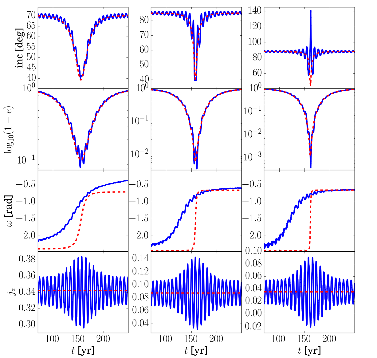
Figure 1: Example of a direct N-body integration (solid blue lines) vs double-averaged secular code (dashed red lines). The inner binary has masses $M_{\odot}$ and $M_{J}$, $a_{1}=1{\rm\ AU},$ $e_{1}=0.001,$ $\Omega_{1}=\pi/4,$ $\omega_{1}=\pi/2$ and $f=0$. The outer mass is $m_{{\rm out}}=3.2655\ M_{\odot}$, where the parameters of the outer orbit are $a_{2}=10\ {\rm AU},$ $e_{2}=0.001,$ (corresponding to $\epsilon_{{\rm SA}}=0.05$) $\Omega_{2}=\omega_{2}=f=0$. Top to bottom: Inclination, eccentricity, argument of pericentre, $j_{z}$. Left to right: Initial inclinations of $i_{{\rm tot}}=70,85,88^{\circ}$, corresponding to DA, SA and N-body regime, respectively. We see that all the orbital elements have a fast fluctuating term, modulated by the secular LK resonance. Even in the DA regime, $e_{\rm max}$ is under-predicted. The strong fluctuations in $j_{z}$ occur near the maximal eccentricity. In N-body regime, the angular momentum flips sign and orbital flips are possible.

2.3 Keplerian perturbations and corrected double averaging

The DA approximation misses perturbations on timescales shorter than the secular timescale, $\tau_{{\rm sec}}$. When the hierarchy is weak, the accumulated errors in neglecting these perturbations could be large. Indeed, such effects have already been shown to be important in various astrophysical systems (Ćuk & Burns, 2004; Antonini & Perets, 2012; Antognini et al., 2014)

It is possible to use the SA equations of motion that depend on the position of the outer orbit, $\boldsymbol{r}_{\rm out}$ (Luo et al., 2016; Liu & Lai, 2018). Luo et al. (2016) discuss the corrections to the double averaging approximation from short-term oscillations. The key parameter that measures the level of the hierarchy and the typical perturbations is the “Single Averaging” (SA) strength ( Eq. 20 of Luo et al., 2016) is

$$\epsilon_{{\rm SA}}\equiv\left(\frac{a_{1}}{a_{{\rm out}}(1-e_{{\rm out}}^{2})}\right)^{3/2}\left(\frac{m_{{\rm{\rm out}}}^{2}}{(m_{1}+m_{{\rm{\rm out}}})m_{1}}\right)^{1/2}=\frac{P_{{\rm out}}}{2\pi\tau_{{\rm sec}}}.$$ (17)

The vectors that describe the binary can be decomposed into the averaged ones $(\bar{\boldsymbol{j}};\ \bar{\boldsymbol{e}})$ that vary slowly on a secular timescale $\tau_{{\rm sec}}$ (Eq. 2), and the fluctuating ones ($\boldsymbol{j}_{f}\equiv\boldsymbol{j}-\bar{\boldsymbol{j}};\ \boldsymbol{e}_{f}\equiv\boldsymbol{e}-\bar{\boldsymbol{e}}$), that vary with a period $\sim P_{{\rm out}}$ . The effects of a weak hierarchy are two-fold:

1. Short term fluctuations in the orbital elements with an amplitude that depend on $\epsilon_{{\rm SA}}$ and the averaged values of $(\bar{\boldsymbol{j}},\bar{\boldsymbol{e}})$:

   $$\mathscr{A}(\epsilon_{{\rm SA}},\bar{\boldsymbol{j}},\bar{\boldsymbol{e}})=\epsilon_{{\rm SA}}\sqrt{C^{2}+S^{2}}\left(1+\frac{2\sqrt{2}}{3}e_{{\rm out}}\right),$$ (18)

   where

   $$C \equiv\frac{3}{8}\left(5\bar{e}_{x}^{2}-5\bar{e}_{y}^{2}-\bar{j}_{x}^{2}+\bar{j}_{y}^{2}\right)$$

   $$S \equiv\frac{3}{8}\left(-10\bar{e}_{x}\bar{e}_{y}+2\bar{j}_{x}\bar{j}_{y}\right).$$ (19)

2. Additional evolution of the averaged vectors $(\bar{\boldsymbol{j}};\ \bar{\boldsymbol{e}})$ themselves. The full equations of motion appear in Appendix A of Luo et al. (2016), which corresponds to the additional effective “corrected double averaging” potential (Eq. 39 of Luo et al., 2016):

   $$\Phi_{{\rm SA}}(\bar{\boldsymbol{j}},\bar{\boldsymbol{e}})=-\epsilon_{{\rm SA}}\frac{Gm_{{\rm out}}a_{1}^{2}}{a_{{\rm out}}^{3}(1-e_{{\rm out}}^{2})^{3/2}}\left(\phi_{{\rm circ}}+e_{{\rm out}}^{2}\phi_{{\rm ecc}}\right)$$ (20)

   where

   $$\phi_{{\rm circ}}(\bar{\boldsymbol{j}},\bar{\boldsymbol{e}}) =\frac{27}{64}\bar{j}_{z}\left\{\frac{1-\bar{j}_{z}^{2}}{3}+8\bar{e}^{2}-5\bar{e}_{z}^{2}\right\}$$ (21)

   $$\phi_{{\rm ecc}}(\bar{\boldsymbol{j}},\bar{\boldsymbol{e}}) =\frac{3}{64}\left\{\bar{e}_{z}(10\bar{j}_{x}\bar{e}_{x}-50\bar{j}_{y}\bar{e}_{y})\right.$$

   $$+\left.\bar{j}_{z}(5\bar{j}_{x}^{2}-\bar{j}_{y}^{2}+65\bar{e}_{x}^{2}+35\bar{e}_{y}^{2})\right\}$$ (22)

Luo et al. (2016) have shown that adding these corrections is more compatible with N-body integrations and it changes the long-term dynamics of particular orbits. Note that adding the corrected potential in Eq. (20) together with the fluctuating terms is equivalent to direct single-averaging (cf. Fig. 3 and 4 of Luo et al. (2016) for comparison).

Previous studies have identified that DA is valid if $\sqrt{1-e_{\rm max}^{2}}\geq 2\pi\epsilon_{\rm SA}$, otherwise SA regime is valid if $\sqrt{1-e_{\rm max}^{2}}\geq 2\pi\epsilon_{\rm SA}^{2}$ (Liu & Lai, 2018). Thus, for eccentricities which exceed the latter limit, direct N-body integration is required (N-body regime). The corrected DA formalism alleviates the need to switch between SA and DA regimes, and both regimes are accounted for via the continuous parameter $\epsilon_{\rm SA}$. Nevertheless, the N-body regime is achieved only when the fluctuation in angular momentum is at least the order of itself (Antonini et al., 2017). We show in sec. 3.3 that our maximal eccentricity formula is valid wherever it is bound.

3 Corrected maximal eccentricity

In this section we calculate the corrected maximal eccentricity attained from the contributions of the single averaging. The initial conditions for eliminating the fluctuating elements and the typical strength of fluctuations is found in sec. 3.1 The contribution from the effective potential is calculated in 3.2, while the fluctuating contribution is calculated in 3.3 We then compare our result with direct N-body realizations.

3.1 Initial conditions and $j_{z}$ fluctuation

In order to compare the SA secular equation with N-body integrations we need the initial conditions to match for the averaged vectors $(\bar{\boldsymbol{j}};\ \bar{\boldsymbol{e}})$. To linear order in $\epsilon_{{\rm SA}}$, the fluctuating terms are a (finite) sum of Fourier components where the lowest period is $P_{{\rm out}}$. We focus on the key parameter $\bar{j}_{z}$.

For zero outer eccentricity $e_{{\rm out}}=0$, the fluctuating term is given by (e.g. Eq. (32) of Luo et al., 2016)

$$j_{z,f}\equiv j_{z}-\bar{j}_{z}=\epsilon_{{\rm SA}}\left(S\sin(2f_{2})-C\cos(2f_{2})\right),$$ (23)

where $C$ and $S$ are given in Eq. (19) and $f_{2}$ is the true anomaly of the outer orbit. For low initial eccentricity, $e\ll 1$, and using the definitions of $\boldsymbol{j}$ (Eq. 5) we get

$$j_{z,f}=-\frac{3}{8}\epsilon_{{\rm SA}}\sin^{2}i_{{\rm tot}}\cos(2\delta),$$ (24)

where $\delta\equiv\Omega_{1}-f_{2}$. Thus, if we want the initial condition to correspond to the averaged $\bar{j}_{z}$ we need to choose the initial angles such that $\delta=(\pi/4+n/2),$ $n=\{0,1,2...\}$.

The fluctuation in $j_{z}$ is maximal where the inner eccentricity is the largest. From Eq. (18), and for highly eccentric orbits, the fluctuation amplitude for $j_{z}$, $\mathscr{A}(\epsilon_{{\rm SA}},\bar{j}\ll 1,\bar{e}\to 1)\equiv\Delta j_{z}$ is

$$\Delta j_{z}=\frac{15}{8}\epsilon_{{\rm SA}}\bar{e}_{{\rm max}}^{2}\cos^{2}\bar{i}_{{\rm min}}=\frac{9}{8}\epsilon_{{\rm SA}}\bar{e}_{{\rm max}}^{2},$$ (25)

where we used the standard value of $\cos^{2}\bar{i}_{{\rm min}}=3/5$. Since the correction is already of order $\mathscr{O}(\epsilon_{{\rm SA}})$, any deviations caused by single-averaging will be at least $\mathscr{O}(\epsilon_{{\rm SA}})$, thus corrections to Eq. (25) from different values of either $\bar{e}_{{\rm max}}$ or $\cos\bar{i}_{{\rm min}}$ will be $\mathscr{O}(\epsilon_{{\rm SA}}^{2})$.

Fig. 1 shows the evolution of the orbital elements of a typical triple system where direct N-body and secular equations of motions are compared . We see that the fluctuations in $j_{z}$ are strongest where the eccentricity approaches $e_{{\rm max}}.$ In addition, choosing $\delta=\pi/4$ guarantees that both $i_{{\rm tot}}$ and $j_{z}$ will be set at their mean values. The actual maximal eccentricity is larger than its averaged value. The eccentricity and $j_{z}$ panels show us that regardless of initial $j_{z}$ and the typical regime (DA, SA or N-body), the eccentricity is always underestimated with similar amplitude. Moreover, if $\Delta j_{z}>j_{z}$, orbital flips are allowed and the eccentricity is stochastic and unbound. In the next sections we calculate the maximal eccentricity taking into account the short-term fluctuations and compare the results with full N-body simulations.

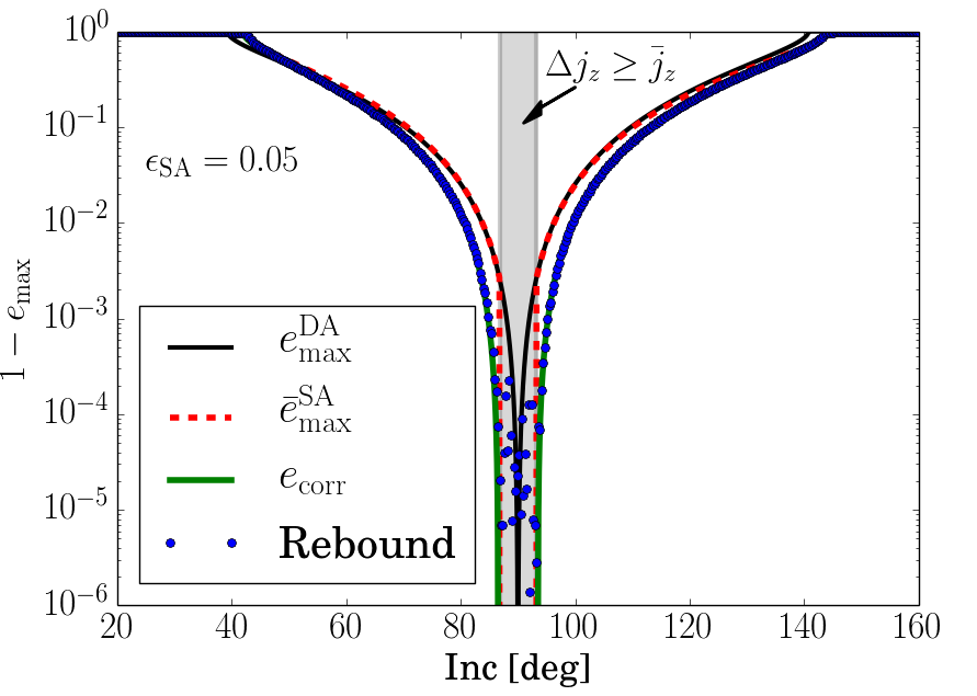
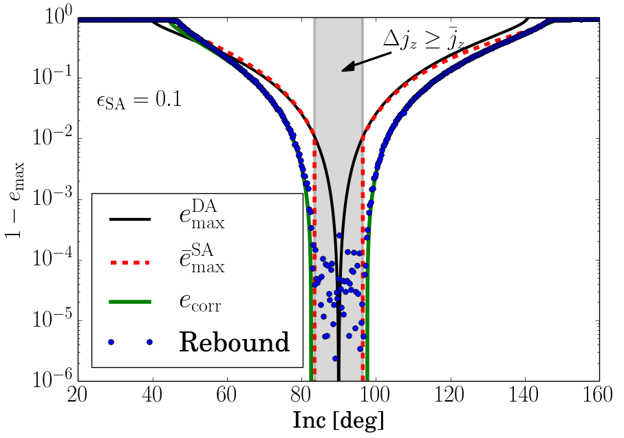
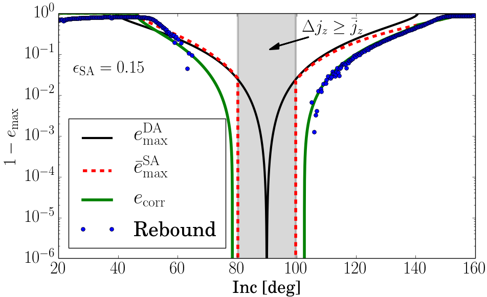
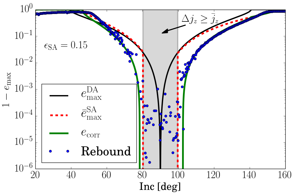
Figure 2: Maximal eccentricity versus initial inclination. We compare corrected averaged secular theory vs. N-body realizations. All simulations start with inner binary of masses $M_{\odot}$ and $M_{J}$, $a_{1}=1{\rm\ AU},$ $e_{1}=0.001,$ $\Omega_{1}=\pi/4,$ $\omega_{1}=\pi/2$ and $f_{1}=0$. The outer orbit is at separation $a_{2}=10\ {\rm AU},$ $e_{2}=0.001,$ $\Omega_{2}=\omega_{2}=f_{2}=0$. Top left: $m_{{\rm out}}=3.2655\ M_{\odot}$ (corresponding to $\epsilon_{{\rm SA}}=0.05$). Top right: $m_{{\rm out}}=10.93\ M_{\odot}$ (corresponding to $\epsilon_{{\rm SA}}=0.1$). Bottom: $m_{{\rm out}}=23.461\ M_{\odot}$ (corresponding to $\epsilon_{{\rm SA}}=0.15$). The end time of all runs is $10^{4}$ times the inner orbit, expect for top right, with end time of $500$ inner orbits. Solid black line is the classical $e_{\rm max}^{\rm DA}$ from standard double-averaged LK mechanism. Dashed red line is the single-averaged corrected eccentricity $\bar{e}_{{\rm max}}^{{\rm SA}}$ given in Eq. (33). Solid green line is the corrected maximal eccentricity after taking into account fluctuating terms in $e_{{\rm corr}}$ given in Eq. (36). Grey area is the allowed zone for orbital flips, where $1-e_{{\rm max}}$ is unbound. For $\epsilon_{{\rm SA}}=0.15$, the system is very close to its Hill stability radius ($a_{1}\approx 0.41r_{\rm H},$ $r_{\rm H}=10(M_{{\rm in}}/3M_{{\rm out}})^{1/3}$), hence highly inclined orbits are unstable on long timescales (Grishin et al., 2017). Bottom left panel shows integrating for shorter times and hence more orbits, which become unstable after longer integrations.

3.2 Maximal single-averaged eccentricity

We are interested in finding $\bar{j}_{{\rm min}}(\bar{j}_{z},\bar{e})\equiv(1-\bar{e}_{{\rm max}}^{2})^{1/2}$ (and therefore $\bar{e}_{{\rm max}}=(1-\bar{j}_{{\rm min}}^{2})^{1/2}$ ) as a function of initial conditions. We obtain it from equating the total potential

$$\Phi_{{\rm tot}}(\bar{\boldsymbol{j}},\bar{\boldsymbol{e}})=\Phi_{{\rm quad}}(\bar{j}_{z},\bar{e},\bar{e}_{z})+\epsilon_{{\rm SA}}\Phi_{{\rm SA}}(\bar{\boldsymbol{j}},\bar{\boldsymbol{e}})$$ (26)

in two points of extreme (minimal and maximal) eccentricities. A similar approach to calculate $j_{{\rm min}}$ in the presence of non-Keplerian forces was used in Liu et al. (2015) and reviewed in sec. 2.2

To first order for circular orbits, $\bar{j}_{z}$ is conserved (Luo et al., 2016) and the (dimensionless) potential depends on

$$\phi_{{\rm tot}}(\bar{\boldsymbol{j}},\bar{\boldsymbol{e}})=\phi_{{\rm quad}}(\bar{j}_{z},\bar{e},\bar{e}_{z})+\epsilon_{{\rm SA}}\phi_{{\rm circ}}(\bar{j}_{z},\bar{e},\bar{e}_{z}).$$ (27)

where $\phi_{{\rm tot}}\equiv\Phi_{{\rm tot}}/\Phi_{0}$. Note that for $e_{{\rm out}}\neq 0$ orbits, $\bar{j}_{z}$ is no longer a constant and we cannot close the equation to obtain the maximal eccentricity. The maximal eccentricity from the additional SA evaluation term is $\bar{e}_{{\rm max}}^{{\rm SA}}.$ Denote the initial mutual inclination by $i_{{\rm tot}}=i_{0}$ and the inner eccentricity is $e_{0}$ . In order to evaluate the potential in Eq. (27) we need to specify $\omega.$ For librating orbits, $\omega=\pi/2$ for both extreme value of the eccentricity (Katz et al., 2011). For small minimal eccentricity, i.e. $e_{0}\ll 1$ the orbit could be circulating, but $\omega$ is not properly defined and plays a role, since the term that contains $\omega$ is proportional to $e^{2}$. Thus, it is safe to take $\omega=\pi/2$ in our evaluations, similarly to Liu et al. (2015).

For the initial conditions stated above, the potential is

$$\phi_{{\rm tot}}(e_{0}) =1+9e_{0}^{2}-3\bar{j}_{z}^{2}-15e_{0}^{2}\cos^{2}i_{0}$$

$$-\epsilon_{{\rm SA}}\frac{27}{8}\bar{j}_{z}\left(\frac{1-\bar{j}_{z}^{2}}{3}+3e_{0}^{2}+5e_{0}^{2}\cos^{2}i_{0}\right).$$ (28)

When the orbit attains its maximal eccentricity, the orbital elements are $e=\bar{e}_{{\rm max}},$ $\cos^{2}i_{{\rm min}}=\bar{j}_{z}^{2}/\bar{j}_{{\rm min}}^{2}$ and $\omega=\pi/2$. The potential is

$$\phi_{{\rm tot}}(\bar{e}_{{\rm max}}) =1+9\bar{e}_{{\rm max}}^{2}-3\bar{j}_{z}^{2}-15\bar{e}_{{\rm max}}^{2}\frac{\bar{j}_{z}^{2}}{\bar{j}_{{\rm min}}^{2}}$$

$$-\frac{27}{8}\epsilon_{{\rm SA}}\bar{j}_{z}\left(\frac{1-\bar{j}_{z}^{2}}{3}+3\bar{e}_{{\rm max}}^{2}+5\bar{e}_{{\rm max}}^{2}\frac{\bar{j}_{z}^{2}}{\bar{j}_{{\rm min}}^{2}}\right).$$ (29)

Equating both terms (Eq. 29 and 28) we get

$$\bar{j}_{{\rm min}}^{2}\left(1-\frac{e_{0}^{2}}{\bar{e}_{{\rm max}}^{2}}\right) =\frac{5}{3}\bar{j}_{z}^{2}\left(1-\frac{j_{{\rm min}}^{2}}{\bar{e}_{{\rm max}}^{2}}\frac{e_{0}^{2}}{j_{{\rm 0}}^{2}}\right)$$

$$+\frac{9}{8}\epsilon_{{\rm SA}} \bar{j}_{z}\left[\bar{j}_{{\rm min}}^{2}\left[1-\frac{1}{3}\frac{e_{0}^{2}}{\bar{e}_{{\rm max}}^{2}}\left(3+5\frac{\bar{j}_{z}^{2}}{j_{{\rm 0}}^{2}}\right)\right]+\frac{5}{3}\bar{j}_{z}^{2}\right].$$ (30)

In the limit of $e_{0}\ll 1,$ $j_{0}\to 1$ and $\bar{j}_{z}\to\cos i_{0}$ we have

$$\bar{j}_{{\rm min}}^{2}-\frac{5}{3}\cos^{2}i_{0}=\frac{9}{8}\epsilon_{{\rm SA}}\cos i_{0}\left(j_{{\rm min}}^{2}+\frac{5}{3}\cos^{2}i_{0}\right),$$ (31)

or solving for $\bar{j}_{\rm min}$:

$$\bar{j}_{{\rm min}}^{2} =\frac{5}{3}\cos^{2}i_{0}\frac{1+\frac{9}{8}\epsilon_{{\rm SA}}\cos i_{0}}{1-\frac{9}{8}\epsilon_{{\rm SA}}\cos i_{0}}$$

$$\approx\frac{5}{3}\cos^{2}i_{0}\left(1+\frac{9}{4}\epsilon_{{\rm SA}}\cos i_{0}\right)+\mathscr{O}(\epsilon_{{\rm SA}}^{2}).$$ (32)

Note that the (averaged) maximal eccentricity in the SA regime is:

$$\boxed{\bar{e}_{{\rm max}}^{{\rm SA}}=\sqrt{1-\frac{5}{3}\cos^{2}i_{0}\frac{1+\frac{9}{8}\epsilon_{{\rm SA}}\cos i_{0}}{1-\frac{9}{8}\epsilon_{{\rm SA}}\cos i_{0}}}}.$$ (33)

For linear terms in $\epsilon_{{\rm SA}}$

$$\bar{e}_{{\rm max}}^{{\rm SA}} \approx\sqrt{1-\frac{5}{3}\cos^{2}i_{0}\left(1+\frac{9}{4}\epsilon_{{\rm SA}}\cos i_{0}\right)}$$

$$=\bar{e}_{{\rm max}}^{{\rm DA}}-\frac{15}{8\bar{e}_{{\rm max}}^{{\rm DA}}}\cos^{3}i_{0}\epsilon_{{\rm SA}}+\mathscr{O}(\epsilon_{{\rm SA}}^{2}).$$ (34)

where the standard DA eccentricity $\bar{e}_{{\rm max}}^{{\rm DA}}$ is defined in Eq. (1).

The critical inclination for the onset of the LK mechanism is obtained in Appendix A

$$\cos i_{{\rm crit}}=\sqrt{\frac{3}{5}}-\frac{27}{40}\epsilon_{{\rm SA}}.$$ (35)

Note that $\bar{e}_{{\rm max}}^{{\rm SA}}$ and $i_{{\rm crit}}$ break the symmetry between prograde and retrograde orbits, since $\cos i_{{\rm crit}}$ is no longer symmetric, which has implications on the general evolution and Hill-stability of the system (Grishin et al., 2017, Appendix A).

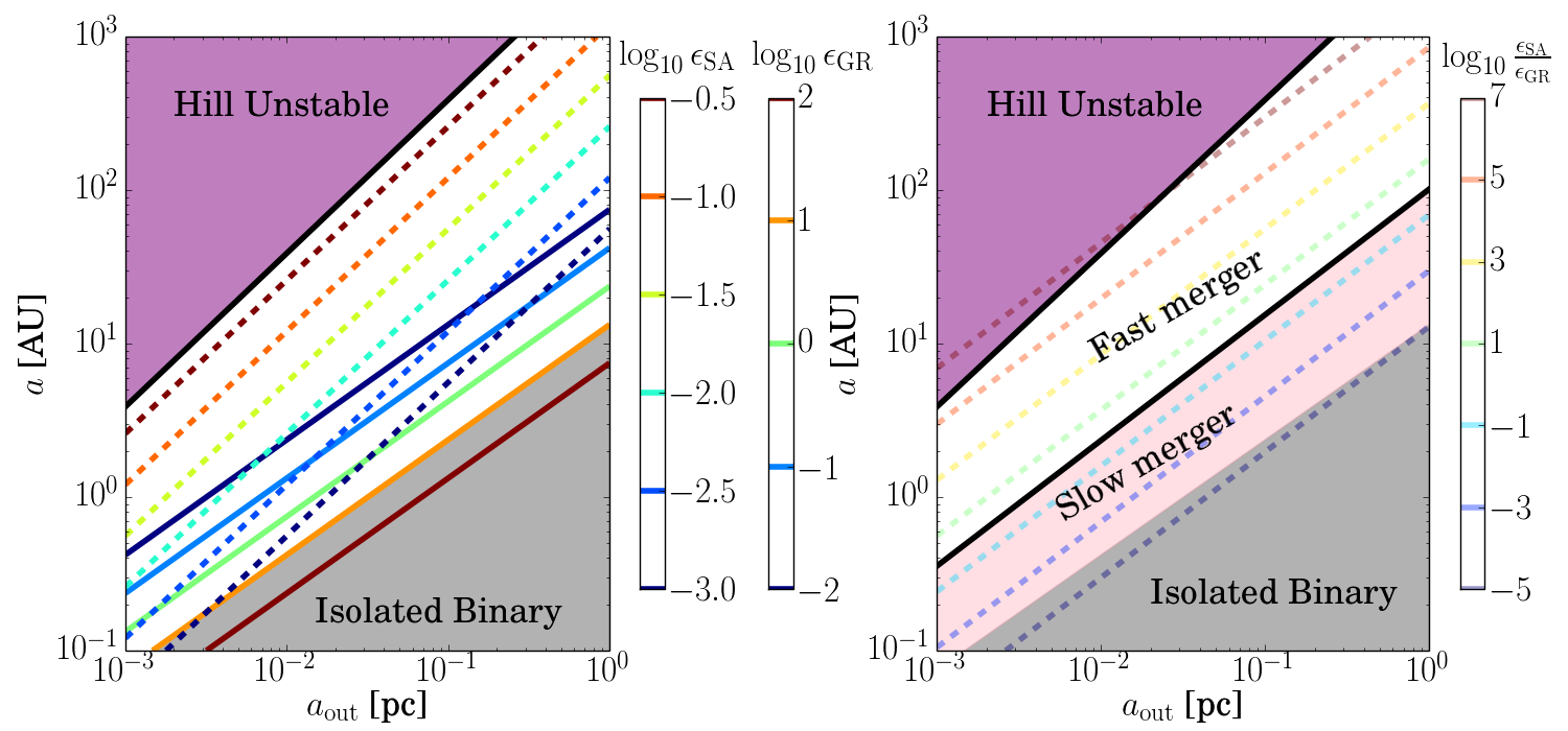
Figure 3: Dimensionless parameters of BH binary as a function of inner and outer separations. Left: Numerical values of $\epsilon_{{\rm GR}}$ (solid) and $\epsilon_{{\rm SA}}$ (dashed) on the $a$, $a_{{\rm out}}$ plane. Purple area (upper left corner) is the region where the binary is Hill unstable, e.g. where $a>r_{{\rm H}}$ where $r_{{\rm H}}=a_{{\rm out}}(m_{{\rm bin}}/3m_{{\rm out}})^{1/3}$ is the Hill radius. Grey area (bottom right corner) is the region where $\epsilon_{{\rm GR}}\geq 10,$ so GR completely quenches eccentricity excitations and binary evolves as an isolated binary. Right: Contours of the ratio $\epsilon_{{\rm SA}}/\epsilon_{{\rm GR}}$. Pink area is the region where $\epsilon_{{\rm GR}}\gg\epsilon_{{\rm SA}}$, thus the maximal eccentricity is never close to unity, so only slow mergers are possible. While area is where $\epsilon_{{\rm SA}}\gg\epsilon_{{\rm GR}},$ thus arbitrary large eccentricities and orbital flips are possible if $\bar{j}_{z}$ is small enough. In this area fast merger (or direct BH-BH collisons) are possible. The dividing line between slow and fast mergers is given by Eq. (45).

3.3 Maximal fluctuating eccentricity

We calculated $\bar{e}_{{\rm max}}^{{\rm SA}}$ from equating the potential at two points with a constant $\bar{j}_{z}$. In reality, $j_{z}$ fluctuates around an averaged value $\bar{j}_{z}$ and a fluctuating amplitude $\Delta j_{z}$ given in Eq. (25). In turn, the eccentricity is also fluctuating around an averaged value $\bar{e}_{{\rm max}}$ and some fluctuation $\delta e$. Since $\phi_{{\rm circ}}\propto\bar{j}_{z}$, when $\bar{j}_{z}\approx\cos i_{{\rm tot}}\ll 1$ is small, the additional term is of order $\mathscr{O}(\bar{j}_{z}\epsilon_{{\rm SA}}),$ therefore we need to take into account second order terms in the expansion of $\delta e_{{\rm max}}$, i.e. keeping terms of order $\mathscr{O}(\epsilon_{{\rm SA}}^{2},\bar{j}_{z}\epsilon_{{\rm SA}})$.

The corrected maximal eccentricity is

$$e_{{\rm corr}} =\bar{e}_{{\rm max}}^{{\rm SA}}+\delta e=\sqrt{1-(\bar{j}_{{\rm min}}-\delta j)^{2}}$$

$$\delta j =\frac{\Delta j_{z}}{\cos i_{{\rm min}}}=\frac{9}{8}\sqrt{\frac{5}{3}}\left(\bar{e}_{{\rm max}}^{{\rm SA}}\right)^{2}\epsilon_{{\rm SA}}.$$ (36)

Since $j_{{\rm min}}\sim\mathscr{O}(\epsilon_{{\rm SA}})$, the leading term is $\delta j\cdot j_{{\rm min}}\sim\mathscr{O}(\epsilon_{{\rm SA}}^{2})$, therefore we need to use a Taylor expansion to second order:

$$|\delta e| =\left.\frac{\partial e_{{\rm max}}}{\partial j}\right|_{j_{{\rm min}}}\delta j_{{\rm min}}+\frac{1}{2}\left.\frac{\partial^{2}e_{{\rm max}}}{\partial j^{2}}\right|_{j_{{\rm min}}}\delta j_{{\rm min}}^{2}$$

$$=\frac{|j_{{\rm min}}|}{e_{{\rm max}}}\delta j_{{\rm min}}+\frac{(\delta j_{{\rm min}})^{2}}{2e_{{\rm max}}^{3}}.$$ (37)

Plugging $j_{{\rm min}}=\bar{j}_{{\rm min}}-\delta j$ and $e_{{\rm max}}=\bar{e}_{{\rm max}}^{{\rm SA}}$ from Eq. (33) and (36) yields

$$\boxed{\delta e=\frac{135}{128}\bar{e}_{{\rm max}}^{{\rm SA}}\epsilon_{{\rm SA}}\left\{\frac{16}{9}\sqrt{\frac{3}{5}|}\bar{j}_{{\rm min}}|+\epsilon_{{\rm SA}}-2\epsilon_{{\rm SA}}\left(\bar{e}_{{\rm max}}^{{\rm SA}}\right)^{2}\right\}}.$$ (38)

where the absolute value of $|j_{{\rm min}}|$ accounts for retrograde orbits.

Note that Antognini et al. (2014) also obtained an expression for the fluctuation in the maximal eccentricity (their Eq. 3). Antognini et al. (2014) used the fluctuation of the orbit’s angular momentum near the maximal eccentricity, previously derived in Ivanov et al., 2005; last Eq. B14). Antognini et al. (2014) have taken incorrect mass dependence and prefactors in their Eq. (3). In appendix B we re-derive the eccentricity fluctuation from the Ivanov et al. (2005) formula and compare to our results. Our new formula, Eq. (38) thus has three new ingredients: the dependence on $e_{{\rm max}}$, namely $\delta e\propto e_{{\rm max}}$, the use of $\bar{e}_{{\rm max}}^{{\rm SA}}$ instead of $\bar{e}_{{\rm max}}^{{\rm DA}}$, and most important is the last term, which is proportional to $\propto\epsilon_{{\rm SA}}\bar{e}_{{\rm max}}^{2}$. We show that Antognini et al. (2014) overestimate the actual fluctuation, while the error is increasing with increasing $\epsilon_{{\rm SA}}$ (see appendix B for details).

Figure 2 shows the comparison of the various prescriptions for the maximal eccentricity with direct N-body integrations. For N-body integrations we use the publicly available code REBOUND (Rein & Liu, 2012). We use IAS15, a fast, adaptive, high-order integrator for gravitational dynamics, accurate to machine precision over a billion orbits (Rein & Spiegel, 2015). Overall, the simulation tends to follow the curve of $e_{{\rm corr}}$ (Eq. 36) For various values of $\epsilon_{{\rm SA}}$. Note that in the region $|\bar{j}_{z}|\leq\Delta j_{z}$, the value of $1-e_{{\rm max}}$ is unbound from below. In this regime, the orbital orientation can flip from prograde to retrograde and vise versa, similarly to the orbital flip in the octupole regime (see Naoz, 2016 and discussion in sec. 5).

One may still be cautious about the validity of Eq. (38). The SA regime breaks down when $\sqrt{1-e_{\rm max}^{2}}\leq 2\pi\epsilon_{\rm SA}^{2}$, since the time spent near $e_{\rm max}$ is shorter than $P_{\rm in}$. However, the eccentricity is bound only if

$$\bar{j}_{z}=\sqrt{\frac{3}{5}(1-e_{\rm max}^{2})}\geq\Delta j_{z}=\frac{9}{8}\epsilon_{\rm SA}.$$ (39)

Thus, the SA equations break down and the eccentricity is bound only if $\epsilon_{\rm SA}>9/(16\pi)\sqrt{5/3}\approx 0.23$. Typical systems are almost always dynamically unstable for such large values of $\epsilon_{\rm SA}$. Thus, in most cases the flip criteria will be satisfied and the eccentricity will be unbound much before the SA equations will breakdown.

To summarize, the corrected maximal eccentricity given in Eq. (36) is the sum of two new terms: the averaged SA value given in Eq. (33) and the extra fluctuating value given in (38) evaluated at the minimum of the instantaneous value of $|j_{z}|$. The formula is in excellent correspondence with direct N-body integrations for all the examined parameters. In the limit $e_{{\rm{\rm max}}}\to 1$, the flip criteria $|\bar{j}_{z}|\leq\Delta j_{z}$ is restored.

4 Applications

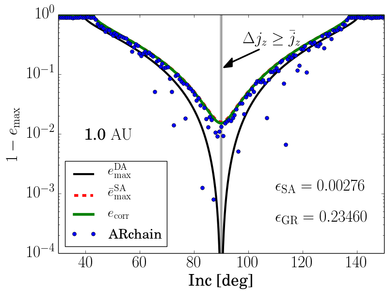
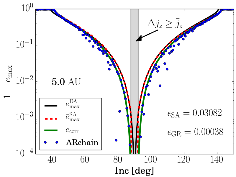
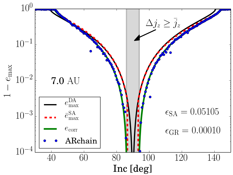
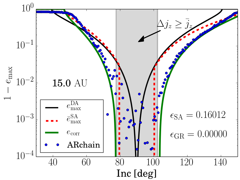
Figure 4: Comparison of analytical estimates with direct integration. We use ARCHAIN code. The initial conditions are $m_{1}=m_{2}=30M_{\odot}$, $m_{3}=4\cdot 10^{6}M_{\odot},$ $a_{2}=0.01\ {\rm pc},$ $\omega_{1}=\pi/2,$ $\Omega_{1}=\pi/4$, $e_{1}=e_{2}=0$. The other angles are zero. Each panel shows the maximal eccentricity as a function of the initial inclination. Each panel has 200 different realization of initial inclination $i_{0}\in[20,160]$ (blue dots), compared with our analytical prediction (green line, Eq. 38, 42). The initial separation is indicated on the left, with calculated valeus of $\epsilon_{{\rm SA}},$ $\epsilon_{{\rm GR}}$ on the right. Top row: $1,5\ {\rm AU},$ bottom row: $7,15\ {\rm AU}.$

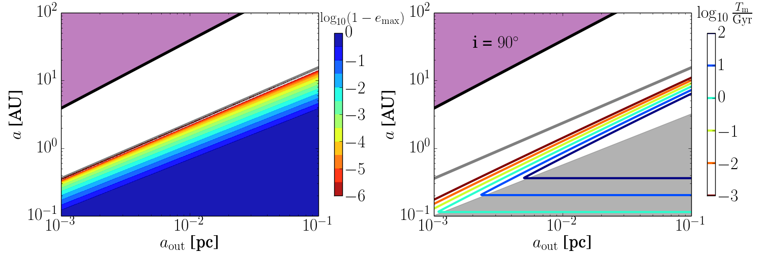
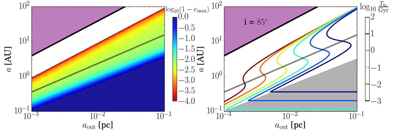
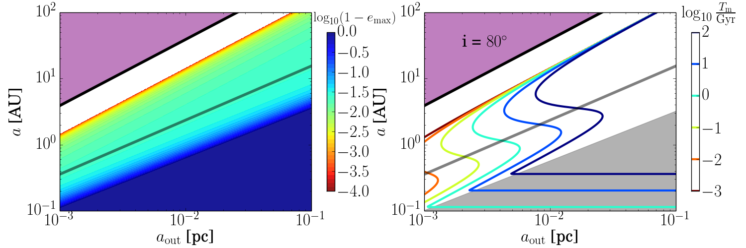
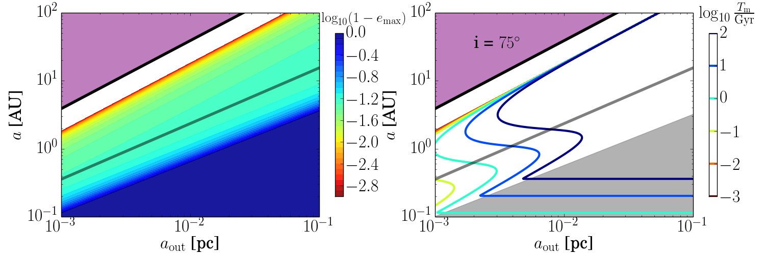
Figure 5: Maximal eccentricy and merger times for binaries in the Galactic Centre. Left panels: Maximal eccentricity as a function of inner and outer semi-major axes. The transparent grey line is Eq. (45), which divides the areas where $e_{{\rm max}}$ is bound and unbound at $i=90^{\circ}.$ Right: Merger times derived from Eq. (40). Grey and purple areas similar to Fig. 3 (i.e. Regions of isolated binary and Hill Unstable orbits, respectively). Top to bottom: inclinations of $90,85,80,75$ degrees, respectively.

4.1 General relativistic corrections and GW mergers

The recent discoveries of high rates of gravitational-Wave (GW) mergers of stellar black holes ($40-213\ {\rm Gpc}^{-3}{\rm yr^{-1}}$, Abbott et al., 2017a, 2016, b) raise the question of their astrophysical origin, and various possibilities exist. These include isolated binary evolution (Belczynski et al., 2016), dynamically formed/evolved binaries in dense stellar systems (e.g. Askar et al., 2017; Rodriguez et al., 2018; Fragione & Kocsis, 2018, and references therein), triple secular evolution of stellar binaries orbiting massive black holes (MBHs; Antonini & Perets, 2012), stellar triple systems (Antonini et al., 2017), and gas-assisted mergers near massive black holes (Bartos et al., 2017; Stone et al., 2017).

One way to decrease the merger time and increase the merger rate is pumping the eccentricity of the inner binary due to LK oscillations. The resulting actual merger time is (Randall & Xianyu, 2018a, b; Liu & Lai, 2018)

$$T_{{\rm m}}=T_{m,0}(1-e_{{\rm max}}^{2})^{3}$$ (40)

where $T_{m,0}$ is the merger time in Eq. (14), with $e=0$. The power comes from the fact that the GW decay rate is $(\dot{a}/a)\propto(1-e^{2})^{-7/2}$, but the binary spends a fraction of $\sim\sqrt{1-e_{{\rm max}}^{2}}$ of its time near $e\sim e_{{\rm max}}.$ Thus, the actual maximal eccentricity is a crutial parameter in determining the actual merger times and rates.

In what follows we derive the analytical result for $e_{{\rm max}}$ in the presence of GR effects and compare to direct simulatioms of N-body and 2.5PN terms that include gravitational wave inspiral in the weak field limit.

4.1.1 Maximal eccentricity

Taking the total potential to be

$$\Phi_{{\rm tot}}=\Phi_{{\rm quad}}+\Phi_{{\rm SA}}+\Phi_{{\rm GR}}$$ (41)

where the potentials are defined in Eqns. (6),(7) and (20). Similarly to sec. 3, evaluating the total potential at extremal values of the eccentricity $e_{{\rm max}}$ and $e_{0}\approx 0$ leads to (the full expression for general $e_{0}$ is in Appendix C)

$$0 =\bar{A}\bar{j}_{{\rm min}}^{2}-8\frac{\epsilon_{{\rm GR}}}{\bar{e}_{{\rm max}}^{2}}\bar{j}_{{\rm min}}-15\bar{j}_{z}^{2}\left(1+\frac{9}{8}\epsilon_{{\rm SA}}\bar{j}_{z}\right)$$

$$\bar{A}(\bar{j}_{z},\bar{e}_{{\rm max}}) \equiv 9-\epsilon_{{\rm SA}}\frac{81}{8}\bar{j}_{z}+8\frac{\epsilon_{{\rm GR}}}{\bar{e}_{{\rm max}}^{2}}.$$ (42)

For $e_{{\rm max}}\to 1,$ Eq. (42) is a simple quadratic equation with the solution

$$\bar{j}_{{\rm min}}=\frac{4\epsilon_{{\rm GR}}\pm\sqrt{16\epsilon_{{\rm GR}}^{2}+15\bar{j}_{z}^{2}\left(1+\frac{9}{8}\epsilon_{{\rm SA}}\bar{j}_{z}\right)\bar{A}_{1}}}{\bar{A}_{1}}$$ (43)

where $\bar{A}_{1}=\bar{A}(\bar{j}_{z},\bar{e}_{{\rm max}}\to 1,)$. In the limit of of $\epsilon_{{\rm GR}}=0$ we get back to Eq. (32). In the limit of $\epsilon_{{\rm SA}}=0$ we retain Eq. (52) of Liu et al. (2015, since $e_{{\rm max}}\to 1$ we implicitly assume $\epsilon_{{\rm GR}}\ll 1$).

In addition, the eccentricity fluctuates by an amount $\delta e$ given be Eq. (38). The actual eccentricity is unbound if

$$\bar{e}_{{\rm max}}^{{\rm SA}}\geq 1-\delta e_{{\rm max}}.$$ (44)

Qualitatively, if $\epsilon_{{\rm GR}}\gg\epsilon_{{\rm SA}}$, the LK eccentricity oscillations will be quenched and orbital flips will be suppressed, while for $\epsilon_{{\rm GR}}\ll\epsilon_{{\rm SA}}$, GR precession is negligible and orbital flips are possible if $\bar{j}_{z}\leq\Delta j_{z}$. In appendix C we show that the critical value that allows unbound eccentricity and orbital flips is

$$\epsilon_{{\rm GR}}\leq\alpha\epsilon_{{\rm SA}},$$ (45)

where $\alpha=81\sqrt{5/3}/64\approx 1.63$. Thus the eccentricity is unbound if $\bar{j}_{z}\leq\Delta j_{z}$ and $\epsilon_{{\rm GR}}\leq\alpha\epsilon_{{\rm SA}}$.

Figure 3 shows the dimensionless parameters $\epsilon_{{\rm GR}}$ and $\epsilon_{{\rm SA}}$ that control the maximal eccentricity. The left panel shows $\epsilon_{{\rm GR}}$ (solid) and $\epsilon_{{\rm SA}}$ (dashed) on the $a$, $a_{{\rm out}}$ plane, while the right panel shows the ratio of $\epsilon_{{\rm SA}}/\epsilon_{{\rm GR}}$. Grey area is the region where $\epsilon_{{\rm GR}}\geq 10$, thus eccentricity excitations are essentially quenched and the binary evolves as an isolated binary. The purple area is the region of phase space where the inner binary is unstable to tidal perturbations of the central object (Hill unstable, $a\geq r_{{\rm H}}=a_{{\rm out}}(m_{{\rm bin}}/3m_{{\rm out}})^{1/3}$). The pink area in the right panel is the region where $\epsilon_{{\rm GR}}\geq\alpha\epsilon_{{\rm SA}}$; the maximal eccentricity in bounded, therefore the merger will take place in the timescale described by Eq. (40). Conversely, the white area allows an unconstrained maximal eccentricity, and thus a direct collision is possible, given enough time and sufficiently large inclination (or low $\bar{j}_{z}$).

Fig. 4 is similar to Fig. 2, but includes the effects of GR. The initial conditions are described in the caption. The modified eccentricity is now given by Eq. (42), while $\delta e_{{\rm max}}$ is unchanged. To include effects of GR we use ARCHAIN code (Mikkola & Merritt, 2006, 2008), a fully regularized code able to model the evolution of binaries of arbitrary mass ratios and eccentricities with extreme accuracy, even over long periods of time. ARCHAIN includes PN corrections up to order PN2.5, which allows to simulate orbital decay and merger due to GW.

The top panels show realizations for $a_{1}=1,5\ {\rm AU}.$ For $1\ {\rm AU}$, GR precession is strong enough to quench extreme eccentricity evolution. Most of the ARCHAIN realizations are slightly below the limiting curve, with a few orbits with extremely high eccentricities, which are probably caused by higher order terms in the PN expansion. For $5\ {\rm AU},$ in the region $i_{0}\sim 60-80\ {\rm deg}$ (or $i_{0}\sim 100-120\ {\rm deg}$ for retrograde cases), additional effects from GR excite the maximal eccentricity beyond our analytical limit. These effects possibly originate from higher terms in the PN expansion, or a PN ’interaction term’ (e.g. Naoz et al., 2013b) which resonantly enhances the maximal eccentricity. Additional study of parameter space is presented in appendix D. Studying these features is beyond the scope of this manuscript and should be studied elsewhere. In the other regions, where the resonances are not excited, the maximal eccentricity does follow our analytic prediction.

The bottom panels show realizations for $a_{1}=7,15\ {\rm AU}.$ In these cases the effects of GR are weak and the maximal eccentricity behaves similarly to the pure N-body case. In the grey area the eccentricity is stochastically distributed, such that longer integration times will decrease $1-e_{{\rm max}}.$

4.1.2 Merger timescale

Figure 5 shows the maximal eccentricity and merger times as a function of the inner and outer separations of the systems. Top to bottom panels show decreasing values of inclination. We see that increasing inclination decreases the available parameter space for fast mergers, since the double-averaged maximal eccentricity is lower. In addition, the overall timescales decrease with increasing inclination, even though the contours of constant merger time have a non-trivial structure.

We can describe the behaviour of equal time curves by the following heuristic arguments. For a typical example, we look at the curve of $T_{{\rm m}}=10\ {\rm Gyr}$, corresponding to an initial $a\approx 0.2\ {\rm AU}$ at inclination of $i=80^{\circ}$. In the area where $\epsilon_{{\rm GR}}\gg 1\gg\epsilon_{{\rm SA}}$ the binary is effectively isolated, and the merger time has the same timescale, regardless of the outer companion. At the point where $\epsilon_{{\rm SA}}\ll\epsilon_{{\rm GR}}\lesssim 1$, the eccentricity is excited, though not to a large value, and the curve makes a sharp turn to the left. At some point $\epsilon_{{\rm GR}}\sim\epsilon_{{\rm SA}}\ll 1$, so the dependence in $\epsilon_{{\rm GR}}$ weakens, and the changes in $e_{{\rm max}}$ are less dramatic. The merger time is dominated by the value of $a$ and the curve takes a turm to the left. At some point the eccentricity is unbound, so the curve takes a final turn to the right, and then asymptotically scales with $\epsilon_{{\rm SA}}\propto(a/a_{{\rm out}})^{3/2}$. The beavior is similar for other contour lines and inclinations.

To summarize, we have shown that the merger time-scales of hierarchical triples can be determined analytically given the initial conditions for systems with comparable mass components where the octupole level of approximation of the triple secular evolution is suppressed. If the distribution functions of the orbital elements are known, the fraction and properties of the merging binaries can be easily estimated and compared to population synthesis simulations; a subject of future work.

Note that the limitations on the allowed time for merger can be significantly shorter than $\sim 10\ {\rm Gyr},$ when taking into account dynamical processes in the Galactic Centre (see Antonini & Perets, 2012 and references therein).

4.2 Formation of Hot Jupiters

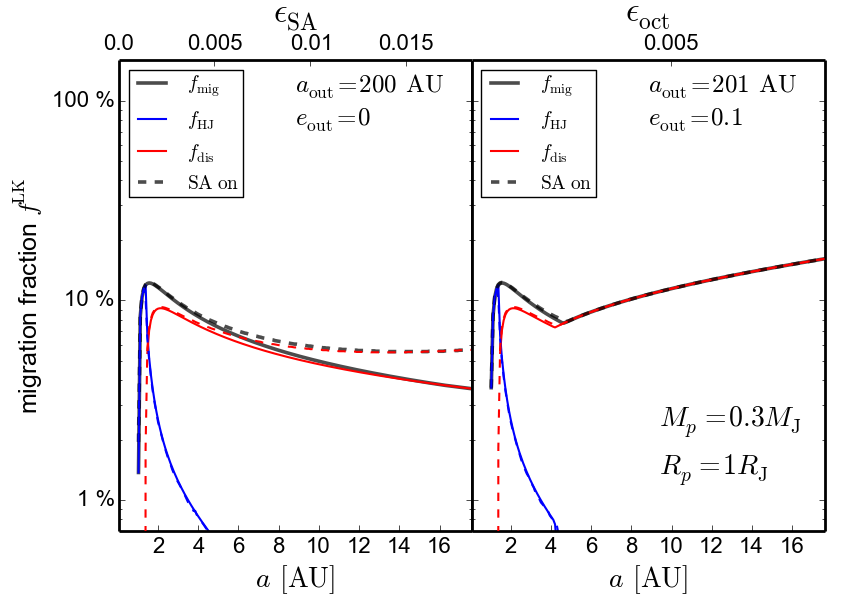
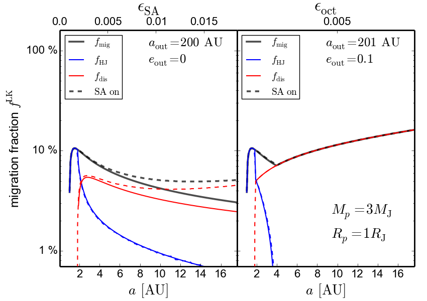
Figure 6: Hot Jupiter migration, disruption and formation rates for a system of masses $M_{\star}=1M_{\odot}$, $M_{{\rm out}}=1M_{\odot}$, with other parameters indicated on the figure. Solid lines are identical to Figs 2 and 3 from Muñoz et al. (2016). Dashed lines are the rates with the inclinaion depends on the corrected maximal eccentricity found in Eq. (38). Left: Rates for low mass planet of $M_{p}=0.3M_{{\rm J}}.$ Right: Rates for massive planet of $M_{p}=3M_{{\rm J}}.$ Plots reproduced from publicly available scripts.

Approximate $\sim 1\%$ of stars have HJ planets (Knutson et al., 2014; giant planets with period $\lesssim 10\ \rm{days}$ or semimajor axis $\lesssim 0.1\ \rm{AU}$). It is difficult to form HJs in-situ, therefore dynamical models of LK cycles coupled to tidal friction have been proposed (Wu & Murray, 2003; Fabrycky & Tremaine, 2007; Naoz et al., 2011b; see introduction and sec. 2.2.3). Populations synthesis studies account for only $15-30\%$ of HJ occurrence rate (Naoz et al., 2012; Petrovich, 2015; Anderson et al., 2016).

Recently, Muñoz et al. (2016) obtained an analytical method for calculating the migration, disruption and HJ formation rate in terms of the hierarchical configuration of the planet and the stellar binary. Muñoz et al. (2016) considered a planet of mass $M_{p}$ and radius $R_{p}$ orbiting a star of mass $M_{\odot}$ with semimajor axis $a$ and eccentrcity $e$, with mutual inclination $i_{\rm tot}$. The star-planet binary orbits a companion of mass $M_{{\rm\odot}}$, semi-major axis $a_{{\rm out}}$ and eccentricity $e_{{\rm out}}.$ Similarly to population synthesis models, Muñoz et al. (2016) sampled from uniform distribution the binary properties (e.g. uniform and independent in $\log a_{\rm out}$, $e_{\rm out}$, $a$, $e$, and $\cos(i_{\rm tot})$) and obtained results which are with population synthesis studies (Petrovich, 2015; Anderson et al., 2016). The overall fraction of forming HJ is not sensitive to the planetary and stellar physical parameters.

The key parameter is the maximal eccentricity, which is excited by LK oscillations, and suppressed by short-range forces (Liu et al., 2015). Planets with pericentre $r_{{\rm disr}}$ (eccentricity $e_{{\rm disr}}$) closer (larger) than

$$r_{{\rm disr}}=a(1-e_{{\rm disr}})=2.7R_{p}\left(\frac{M_{\star}}{M_{p}}\right)^{1/3}$$ (46)

will be disrupted, while planets with pericentre $r_{{\rm mig}}$ (eccentricity $e_{{\rm mig}}$) closer (larger) than

$$r_{{\rm mig}} =a(1-e_{{\rm mig}})$$

$$\approx 1.16\left(\frac{Gk_{2p}\tau_{L}}{M_{p}a}\right)^{1/7}M_{\star}^{2/7}R_{p}^{5/7}\tau_{{\rm dis}}^{1/7}(e_{\rm mig})$$ (47)

will migrate within a timescale $\tau_{{\rm dis}}(e_{\rm mig})$, defined in Eq. (16; cf. exact definition in Muñoz et al., 2016 their Eq. (8) and (9)). Here $k_{2p}$ is the Love number and $\tau_{L}$ is the lag time discussed in sec. 2.2.3.

Similarly to sec. 2.2, (Muñoz et al., 2016) found the maximal eccentricity from comparing the total potential

$$\Phi_{{\rm tot}}=\Phi_{{\rm quad}}+\Phi_{{\rm GR}}+\Phi_{{\rm tide}},$$ (48)

and found the migration, disruption and HJ formation rates for a given binary configuration by taking $f=\arccos(i_{\rm crit})$, where $i_{\rm crit}$ is the critical inclination required to satisfy the disruption or migration radius (Eq. 46 and 47 respectively), while the HJ formation rate is their difference.

Here we examine how our new formula for the maximal eccentricity changes the results. In our case, we add $\Phi_{\rm SA}$ to the total potential, which yields an the implicit equation that determines the maximal eccentricity (in the limit $e_{0}\to 0$):

$$\frac{3}{5}\bar{j}_{{\rm min}}^{2} =\bar{j}_{z}^{2}+\frac{8}{15}\frac{\epsilon_{{\rm GR}}}{\bar{e}_{{\rm max}}^{2}}\left(\bar{j}_{{\rm min}}-\bar{j}_{{\rm min}}^{2}\right)$$

$$+\frac{8}{225}\frac{\epsilon_{{\rm tide}}}{\bar{e}_{{\rm max}}^{2}}\left(\frac{1+3\bar{e}_{{\rm max}}^{2}+3\bar{e}_{{\rm max}}^{4}/8}{8\bar{j}_{{\rm min}}^{7}}-\bar{j}_{{\rm min}}^{2}\right)$$

$$+\epsilon_{{\rm SA}}\frac{9}{8}\bar{j}_{z}\left[\frac{3}{5}\bar{j}_{{\rm min}}^{2}+\bar{j}_{z}^{2}\right].$$ (49)

The first two terms appear in Eq. (18) of Muñoz et al. (2016), the last term is new.

In order to calculate the migration rates, we use the publicly available script from Muñoz et al. (2016). We use the same choice of parameters as in Muñoz et al. (2016, $k_{2p}=0.37,$ $\tau=0.1{\rm\ s},$ $M_{\star}=M_{\odot}$, $M_{p}=M_{J}$, $R_{p}=R_{J}$), and migration time of $\tau_{{\rm dis}}=1\ {\rm Gyr}$, We change the prescription for the critical inclination by numerically solving Eq. (12), for $\bar{e}_{{\rm max}}^{{\rm SA}}\equiv\sqrt{1-\bar{j}_{{\rm min}}^{2}},$ and adding $\delta e_{{\rm max}}$ from Eq. (38). We then scan the possible grid of inclination range until we find the critical inclination $i_{c}$ for which $e_{\rm corr}=\bar{e}_{{\rm max}}^{{\rm SA}}(i_{c})+\delta e_{{\rm max}}(i_{c})\geq e_{{\rm crit}}$, where $e_{{\rm crit}}=e_{{\rm disr}}$ for disruption and $e_{{\rm crit}}=e_{{\rm mig}}$ for migration. There is one to one correspondence between $e_{\rm corr}$ and $i_{c}$ for prograde inclinations. We tried using retrograde inclinations and got essentially the same results, since the dominating enhancement comes from $\delta e$, which is symmetric in $\cos{i}$.

In Fig. 6 we show the modified rates of the migration, disruption and HJ formation as a function of the semi-major axis of the planet. In both panels we see that for closer planets, the effects of single-averaging are suppressed and the results are identical to those obtained from the double averaged case. This is because i) $\epsilon_{{\rm SA}}$ is small and ii) short-range forces are stronger. As we increase the separation of the planet, the effects of short-range forces decrease, and $\epsilon_{{\rm SA}}$ increases. At some point, the SA fraction rates start to diverge from their DA values and increase. We thus expect an increase of the migration rates for the outermost planets (or of the least hierarchical system). Remarkably, both the migration and disruption rates increase, but the total HJ formation rate is unchanged. This is because of the narrow range of maximal eccentricities that needs to be satisfied for efficient HJ formation.

For eccentric outer binaries, the octupole evolution dominates throughout the parameter range and the corrected maximal eccentricity has no effect on the total rates. The caveat is that the detailed octupole and SA evolution could be different and more work is required in order to check the consistency of the model. Changing the binary separation should not significantly affect the results (see Appendix E.

To summarize, the total rate of migration and disruption of HJ increases, but not the total HJ formation rate. Thus, taking SA effects does not improve the total formation rate of HJ, but it can increase the rate and observed distributions of migrating warm Jupiters, with separations of $\sim 0.1-1{\rm AU}$ and eccentricity $e_{p}\geq 0.1$.

5 Limitations and Caveats

Outer eccentricity and octupole evolution:

Our calculation is exact for circular outer orbits. If the outer eccentricity is non-zero, i.e. $e_{{\rm out}}\neq 0$ then the width of the fluctuations increases (cf. Eq. 18), and the width of the fluctuation in the eccentricty $\delta e_{{\rm max}}$ is changed (e.g. Luo et al., 2016; Haim & Katz, 2018). The results can be retained for binaries of equal mass.

The more acute effect occurs when the components of the inner binary have extreme mass ratios. In this case, perturbations from the octupole term cause a chaotic evolution, and may give rise to extreme eccentricities and orbital flips (Ford et al., 2000; Katz et al., 2011; Lithwick & Naoz, 2011; Naoz et al., 2011a; Li et al., 2014; Naoz, 2016). The strength of the octupole term is parametrized by the octupole parameter $\epsilon_{{\rm oct}}\equiv(a/a_{{\rm out}})e_{{\rm out}}/(1-e_{{\rm out}}^{2})$.

It is unclear how the combined effects of the octupole term and the single-averaging term change the evolution of the system. On the one hand, octupole evolution drives the system to a large eccentricity given sufficiently large mutual inclinations. The larger $\epsilon_{{\rm oct}}$ is, the smaller is the required mutual inclination. Thus, it is expected that when $\epsilon_{{\rm oct}}\gtrsim\epsilon_{{\rm SA}}$, the octupolar evolution is restored Luo et al. (2016). In addition, the extra fluctuation in $j_{z}$ should result in more of the phase space being subjected to orbital flips and extreme evolution. On the other hand, some systems do not reach extreme eccentricities, even though the same system could acquire an orbital flip in the DA approximation (cf. Fig 1. of Luo et al., 2016). The actual orbital flip sensitively depends on the initial conditions. Studying the corrections to the flip criteria in the octupole regime is beyond the scope of this paper.

Beyond test particle limit:

We focused on the test particle limit, namely when the outer angular momentum dominates. In the quadrupole approximation, there is still a conserved quantity which depends $j_{z}$ and the inner-to-outer angular momentum ratio (Katz & Dong, 2012; Naoz et al., 2013a; Haim & Katz, 2018; Liu & Lai, 2018), but the behaviour is more complicated. Recently, Liu & Lai (2018) obtained the maximal eccentricity similarly to sec. 2.2 and found that the peak inclination for $e_{\rm max}\to 1$ is shifted to retrograde orbits, and breaks the symmetry. If would be interesting investigate to non-test particle case, a subject of future work.

N-body integrations:

A major limitation is the finite time of integration. Some of the eccentricities could increase for longer integration times, and the overall stability of the system could be questionable. Most notably, in the area where the orbit could flip, some of the attained eccentricities could be lower. The actual maximal eccentricity in this case could depend on the final time of integration and expected to be distributed similarly to record statistics (N. Haim, private communication).

Critical inclination and higher order terms:

Fig. 2 shows that for $\epsilon_{\rm SA}\gtrsim 0.1$ the critical inclination for LK resonance deviates from the predicted value in Eq. (35). The difference is probably from high-order terms in $\epsilon_{\rm SA}$ studied in Ćuk & Burns (2004) and Grishin et al. (2017), and/or in additional terms in the multipole expansion that do not vanish for $e_{\rm out}=0$ (cf. Eq. A120 in Hamers & Portegies Zwart, 2016). In addition, there is a difference of $\sim 15\ \%$ between the linear estimate of Eq. (35) and the linear estimate in Grishin et al. (2017). We refer to appendix A for discussion and possible solutions.

6 Summary

In this paper we studied the effects of short-term perturbations on a mildly hierarchical triple system, together with already studied non-Keplerian perturbations (e.g. general relativity and tides). We focused on the maximum eccentricity, a key parameter that determines the result of many short-range interactions and subsequent evolution of the system. Our result can be summarized as follows:

1. The strength of the perturbations and typical corrections are encapsulated in the hierarchy strength (single-averaged, SA) parameter $\epsilon_{{\rm SA}}$ (Eq. 17).

2. The critical inclinations for the onset of the Lidov-Kozai mechanism change according to Eq. (35), and the overall maximal eccentricity is increased according to Eqns. (33), (36) and (38). The new formula is robust, reproduces the orbital flip criteria, is in good agreement with N-body integrations, and corrects previous work, which has overestimated the eccentricity fluctuations. The main advantage of our calculation is retaining the secular approach, allowing for an efficient computaional approach and better analytic understanding. The double-averaging approximation is not breaking down, but rather is corrected for, such that lesser hierarchies are correctly accounted for.

3. When general relativistic effects are included, they tend to add extra precession and quench the secular Lidov-Kozai eccentricity excitations. We find the maximal eccentriciy with additional general relativistic precession in Eq. (42) and the conditions for orbital flip in Eq. (45). We compare to N-body integrations which include 2.5PN effects and find that our formulae underestimate the maximal eccentricity in some cases, but overall it is in good agreement. We manifest our results by finding the merger time for black-hole binaries in the Galactic Centre and argue that the rate or black-hole mergers due to emission of gravitational waves should be larger when accounting for non-secular effects. In addition, we found a regime where the maximal eccentricity is unconstrained, direct collisions and/or eccentric mergers of binary black holes are possible, similar to direct collisions of white-dwarfs found by Katz & Dong (2012).

4. We apply our results to hot-Jupiter formation rates. We include tidal effects and find the maximal eccentricity in this case in Eq. (49). We incorporate our new maximal eccentricity in a recent analytical model, and find that the total migration rate and the disruption rate are increased, but the rate of Hot-Jupiter formation is unchanged. Nevertheless, the rate for Warm-Jupiter migration can increase and the underlying observed distributions of migrating warm Jupiters and their properties are altered, namely Warm-Jupiters could migrate from further out separations and achieve larger eccentricities.

Appendix A. Critical inclination and Hill stability

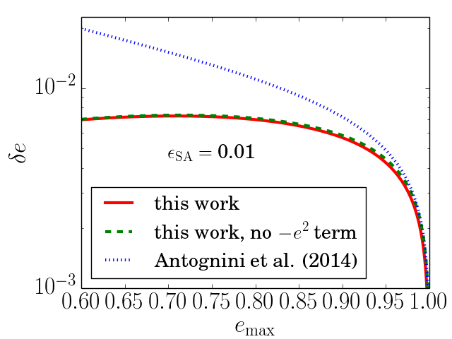
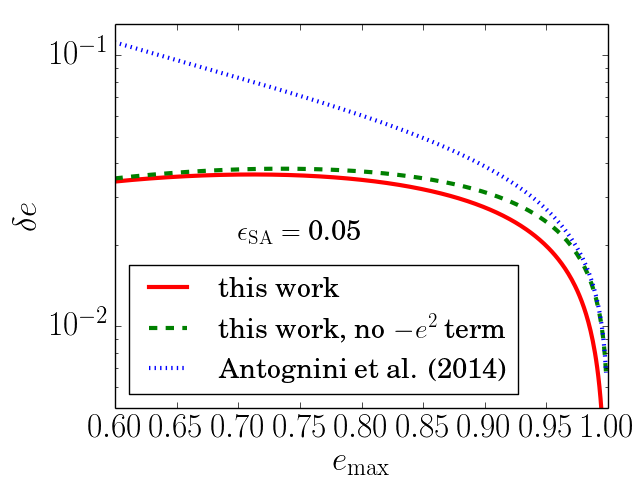
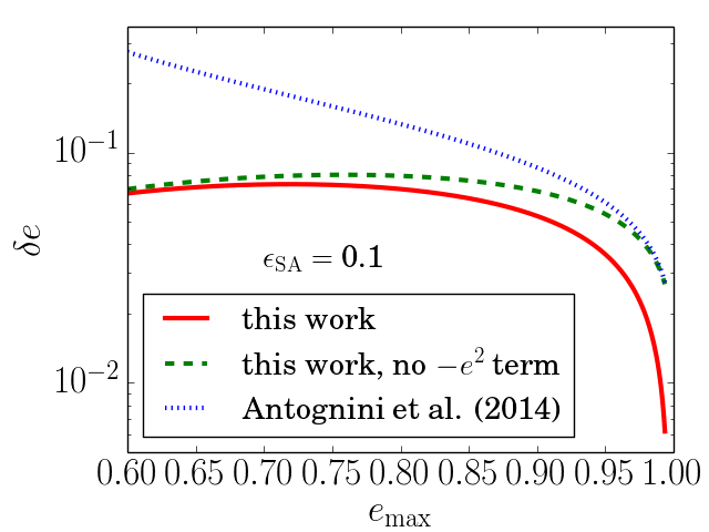
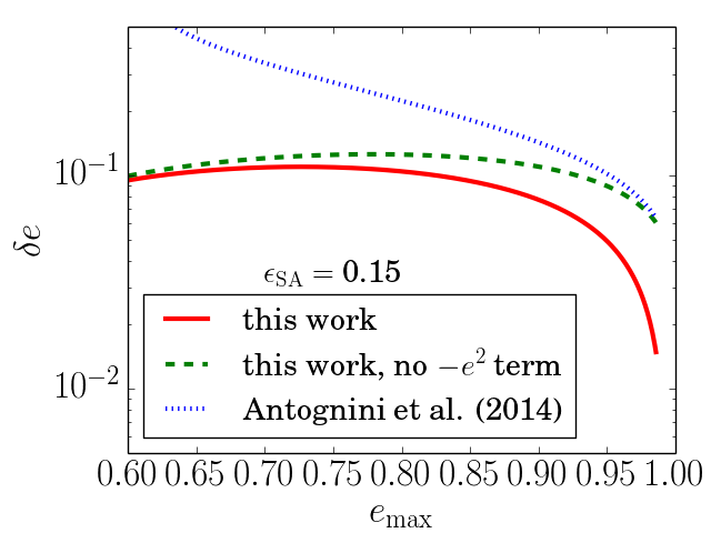
Figure 7: Comparison of our result and Antognini et al. (2014) for various values of $\epsilon_{{\rm SA}}.$ Each panel shows the resulting fluctuation as a function of the (double averaged) maximal eccentricity. Solid red is our Eq. (38), dashed green is the same equation, but without the last term, dotted blue is Eq. (63) (i.e. the corrected version of Antognini et al. (2014)). In each panel, the maximal eccentricity evaluated is such that $j_{{\rm min}}$ is not smaller than $\Delta j_{z}=9\epsilon_{{\rm SA}}/8,$ otherwise orbital flip are possible and the eccentricity is unbound. Neglecting the $\epsilon_{{\rm SA}}e^{2}$ term leads to convergence to Antognini et al. (2014)’s result for large eccentricity. Generally, Antognini et al. (2014) overestimates the fluctuation.

For finding the critical inclination, setting $\bar{j}_{{\rm min}}=1^{-}$ (or $\bar{e}_{\rm max}=0^{+}$) in Eq. (32) yields

$$1 =\frac{5}{3}\cos^{2}i_{{\rm crit}}\frac{1+\frac{9}{8}\epsilon_{{\rm SA}}\cos i_{{\rm crit}}}{1-\frac{9}{8}\epsilon_{{\rm SA}}\cos i_{{\rm crit}}}.$$ (50)

This is an implicit equation. Setting $x\equiv\cos i_{{\rm crit}}$ we have an implicit equation

$$F(x,\epsilon_{{\rm SA}})=\frac{5}{3}x^{2}\frac{1+\frac{9}{8}\epsilon_{{\rm SA}}x}{1-\frac{9}{8}\epsilon_{{\rm SA}}x}-1=0,$$ (51)

where the local solution at $\epsilon_{{\rm SA}}=0$ is $x_{0}=\sqrt{3/5}$. Thus, implicit function theorem allows us to get the first order derivative:

$$\frac{dx}{d\epsilon_{{\rm SA}}} =-\left.\frac{\partial F/\partial\epsilon_{{\rm SA}}}{\partial F/\partial x}\right|_{x=x_{0};\ \epsilon_{{\rm SA}}=0}=-\frac{9}{8}x_{0}^{2}=-\frac{27}{40},$$ (52)

thus

$$x(\epsilon_{{\rm SA}}) =x_{0}+\frac{dx}{d\epsilon_{{\rm SA}}}\epsilon_{{\rm SA}}$$

$$\cos i_{{\rm crit}} =\sqrt{\frac{3}{5}}-\frac{27}{40}\epsilon_{{\rm SA}}.$$ (53)

We can compare with our results in Grishin et al. (2017). Their expansion in the inclinations is:

$$i_{{\rm crit}}=i_{0}+mi_{1},$$ (54)

where $m\equiv\epsilon_{{\rm SA}}$ in the Hill case. The linear correction is

$$\cos i =\cos(i_{0}+mi_{1})=\cos i_{0}\cos(mi_{1})-\sin i_{0}\sin(mi_{1})$$

$$=\cos i_{0}-\sin i_{0}i_{1}m,$$ (55)

therefore

$$i_{1}=\frac{27}{40\sin i_{0}}=\frac{27}{40\sqrt{2/5}}=1.067\ {\rm rad},$$ (56)

In Grishin et al. (2017) we found that the linear correction from Eq. (10) is $i_{1}=1.24\ {\rm rad},$ and the linear term from the polynomial fit is $i_{1}=1.17\ {\rm rad}$, which results in errors of $\sim 15\%$ and $\sim 10\%,$ respectively.

The reason is probably lies in the definition of ’LK resonance’. In Grishin et al. (2017) we found the inclination for which the pericentre librates, namely the condition $d\omega/dt\approx 0$ on average, while here in deriving Eq. (35) we strictly assumed $\omega=\pi/2$ and looked for a solution for Eq. (33) with $e_{\rm max}=0^{+}$. We suspect that Eq. (53) finds the ’bifurcation’ where a fixed point in $e-\omega$ space appears near $e\approx 0$, whereas Eq. (10) of Grishin et al. (2017) describes where librating solutions are wide spread, and the fixed point is at large eccentricity. Thus, slightly higher inclination is required to satisfy Eq. (10) of Grishin et al. (2017). Future studies may better resolve this issue

B. Comparison to Antognini et al. (2014)

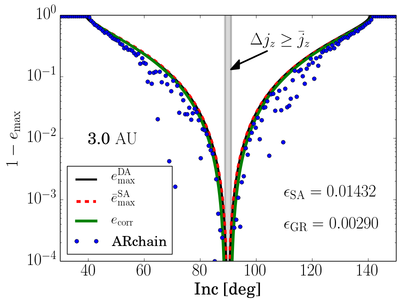
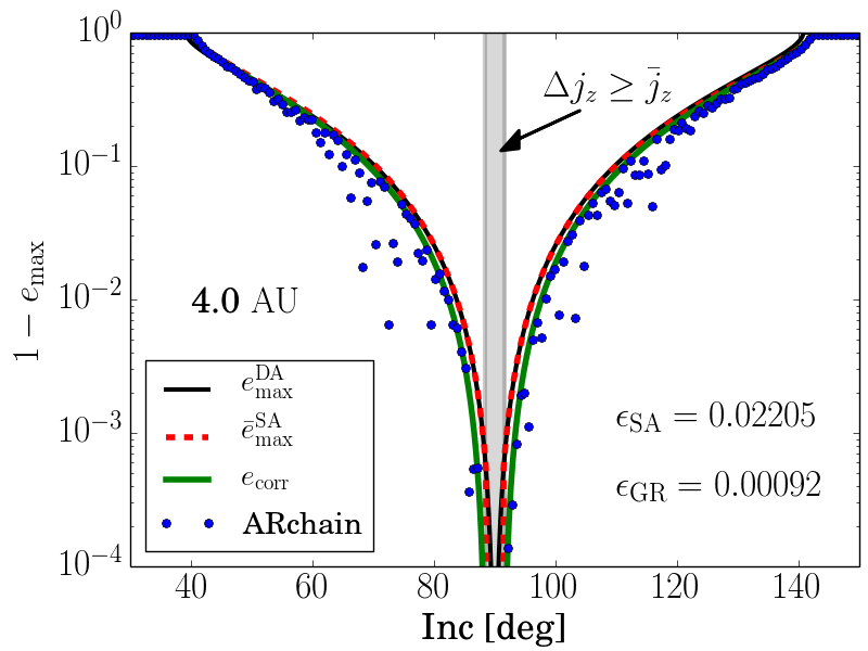
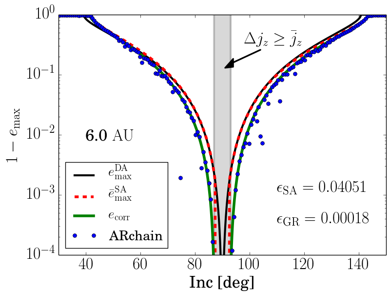
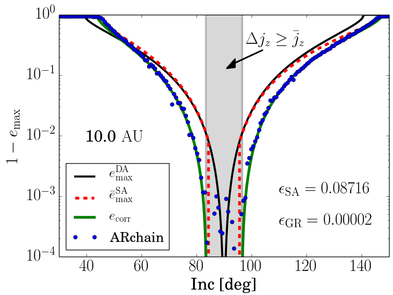
Figure 8: Same as Fig. 4, but with different inner separations. In each panel, the inner binary separation is $3,4,6$ and $10\ {\rm AU}$ for top left, top right, bottom left and bottom right, respectively.

Here we compare our formula of the maximal eccentricity (38) to Antognini et al. (2014). We start from the result of Ivanov et al. (2005) where the change in the angular momentum near the maximum eccentricity is

$$\Delta L=\frac{15}{8}\cos i_{{\rm min}}q\left(\frac{a}{a_{{\rm out}}}\right)^{2}\sqrt{Gm_{1}a_{{\rm out}}},$$ (57)

where $q=m_{{\rm out}}/m_{1}$ is assumed to be small. It appears that Antognini et al. (2014) have confused the mass ratio $q$ in their result, together with additional incorrect prefactors. Note that the change in the normalized angular momentum $\Delta j$ is

$$\Delta j=\frac{\Delta L}{L_{{\rm in,0}}}=\frac{15}{8}\cos i_{{\rm min}}\epsilon_{{\rm SA},}$$ (58)

where $L_{{\rm in,0}}=\sqrt{Gm_{1}a}$ and $\epsilon_{{\rm SA}}=q(a/a_{{\rm out}})^{3/2}$ in the limit of $e_{{\rm out}}=0$ and $q\ll 1$. Comparing to

$$\Delta j_{z}=\Delta j\cdot\cos i_{{\rm min}}=\frac{15}{8}\cos^{2}i_{{\rm min}}\epsilon_{{\rm SA}}$$ (59)

we get the same result of our Eq. (38) if $\bar{e}_{{\rm max}}\approx 1$. Thus, we expect to converge to Ivanov et al. (2005) in this limit.

The eccentricity is

$$e=\sqrt{1-\frac{L_{{\rm in}}^{2}}{Gm_{1}a}},$$ (60)

which is simply a restatement of the expression for the angular momentum $L_{{\rm in}}=\sqrt{1-e^{2}}L_{{\rm in,0}}$. The fluctuation is

$$\delta e =-e+\sqrt{1-\left(\frac{L_{{\rm in}}+\Delta L}{L_{{\rm in,0}}}\right)^{2}}$$

$$=-e+\sqrt{1-\left(\sqrt{1-e^{2}}+\frac{15}{8}\cos i_{{\rm min}}\epsilon_{{\rm SA}}\right)^{2}},$$ (61)

which is essentially Eq. (3) of Antognini et al. (2014), up to normalization factors and corrected mass ratio. Taking $\cos i_{{\rm min}}=\sqrt{3/5}$, $j_{{\rm min}}\equiv\sqrt{1-e^{2}}$ we get

$$\delta e=-e+\sqrt{e^{2}-\frac{15}{4}\sqrt{\frac{3}{5}}j_{{\rm min}}\epsilon_{{\rm SA}}-\frac{135}{64}\epsilon_{{\rm SA}}^{2}}.$$ (62)

Note that the correction is in the order of $\mathscr{O}(\epsilon_{{\rm SA}}^{2}),\mathscr{O}(j_{{\rm min}}\epsilon_{{\rm SA}})$, as expected. Taking $e\approx 1$ and expanding the square root we have

$$\delta e \approx-e+e\left(1-\frac{15}{8}\sqrt{\frac{3}{5}}j_{{\rm min}}\epsilon_{{\rm SA}}-\frac{135}{128}\epsilon_{{\rm SA}}^{2}\right)$$

$$=-\frac{135}{128}\epsilon_{{\rm SA}}\left(\frac{16}{9}\sqrt{\frac{3}{5}}j_{{\rm min}}+\epsilon_{{\rm SA}}\right).$$ (63)

In the limit of $\bar{e}_{{\rm max}}\approx 1$, $j_{{\rm min}}$ is small, thus taking $j_{{\rm min}}=\sqrt{1-\bar{e}_{{\rm max}}}$ leads to a large error, since the fluctuation $\delta j$ could be comparable to $j_{{\rm min}}$. Indeed, when we compare Eq. (63) to our Eq. (38), the last term is missing. Taking $j_{{\rm min}}=\bar{j}_{{\rm min}}-\delta j$ where $\delta j$ is given in Eq. (63) reproduces the right result in the large $e_{{\rm max}}$/ small $j_{{\rm min}}$ limit.

Figure 7 compares the fluctuations found in Antognini et al. (2014) (with our corrected version, blue dotted lines), our work (solid red), and our work without the extra term (dashed green). Overall, Antognini et al. (2014) overestimate the eccentricity fluctuation. The error increases with increasing $\epsilon_{{\rm SA}}.$ In Antognini et al. (2014), their $\epsilon_{{\rm SA}}\approx 0.017$, therefore it is hard to distinguish between different results, although it is evident in their Fig. 1 that their analytic envelope is indeed overestimating the actual fluctuations.

C. Maximal eccentricity with GR precession

From the comparison of the total potential (41) we have for general $e_{0}$:

$$9(\bar{e}_{{\rm max}}^{2}-e_{0}^{2})=15\left(\frac{\bar{e}_{{\rm max}}^{2}\bar{j}_{z}^{2}}{\bar{j}_{{\rm min}}^{2}}-e_{0}^{2}\cos^{2}i_{0}\right)+8\epsilon_{{\rm GR}}\left(\frac{1}{\bar{j}_{{\rm min}}}-\frac{1}{j_{0}}\right)$$

$$+\frac{27}{8}\epsilon_{{\rm SA}}\bar{j}_{z}\left[3(\bar{e}_{{\rm max}}^{2}-e_{0}^{2})+5\left(\frac{\bar{e}_{{\rm max}}^{2}\bar{j}_{z}^{2}}{\bar{j}_{{\rm min}}^{2}}-e_{0}^{2}\cos^{2}i_{0}\right)\right],$$ (64)

where $j_{0}=\sqrt{1-e_{0}^{2}}$ .

In the limit of $\bar{j}_{z}\to 0,$ $\epsilon_{{\rm GR}}\ll 1$ and $\bar{e}_{{\rm max}}^{{\rm SA}}\to 1$ we have

$$\bar{j}_{{\rm min}} =\frac{4\epsilon_{{\rm GR}}\pm\sqrt{16\epsilon_{{\rm GR}}^{2}+135\bar{j}_{z}^{2}}}{9},$$

$$\delta e_{{\rm max}} =\frac{135}{128}\epsilon_{{\rm SA}}\left(\frac{16}{9}\sqrt{\frac{3}{5}}|\bar{j}_{{\rm min}}|-\epsilon_{{\rm SA}}\right).$$ (65)

For $\bar{j}_{z}\ll\epsilon_{{\rm GR}}$, we get Eq. (65) for $e_{{\rm lim}}\equiv(1-\bar{j}_{{\rm min}}^{2})^{1/2}\approx 1-(32/81)\epsilon_{{\rm GR}}^{2}$ (or $\bar{j}_{{\rm min}}=8\epsilon_{{\rm GR}}/9$). Since the condition for a prograde-retrograde flip (Eq. 66) is $\bar{j}_{{\rm min}}\lesssim\Delta j_{z}/\cos i_{{\rm min}}=9\sqrt{5/3}\epsilon_{{\rm SA}}/8$, we plug it in the expression for $\delta e_{{\rm max}}.$ Putting everything into Eq. (44) we then have

$$\epsilon_{{\rm GR}}\leq\alpha\epsilon_{{\rm SA,}}$$ (66)

where $\alpha=81\sqrt{5/3}/64\approx 1.63$. Thus the eccentricity is unbound if $\bar{j}_{z}\leq\Delta j_{z}$ and $\epsilon_{{\rm GR}}\leq\alpha\epsilon_{{\rm SA}}$.

Note that this derivation demonstrates the need for second order terms is $\delta e_{{\rm max}}$. A more direct derivation it to compare $\bar{j}_{{\rm min}}=8\epsilon_{{\rm GR}}/9$ from the limiting eccentricity with the fluctuation $\Delta j_{z}/\cos i_{{\rm min}}=9\sqrt{5/3}\epsilon_{{\rm SA}}/8.$

D. ARCHAIN realization with additional parameters

Fig. 8 shows additional realizations of the parameter space using ARCHAIN

E. HJ formation with different binary separations

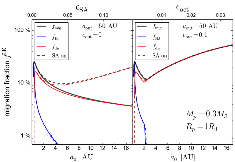
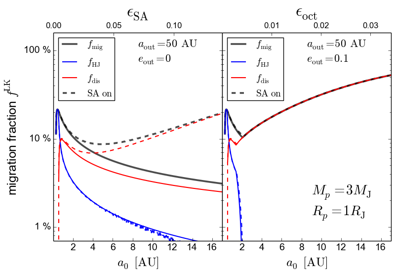
Figure 9: Same as Fig. 6 but with $a_{{\rm out}}=50\ {\rm AU}$.

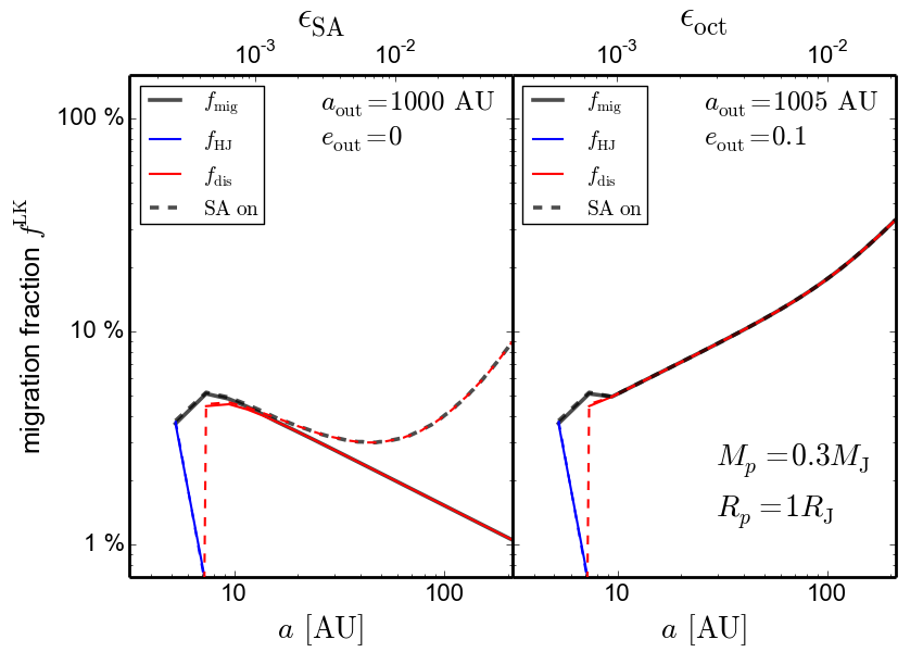
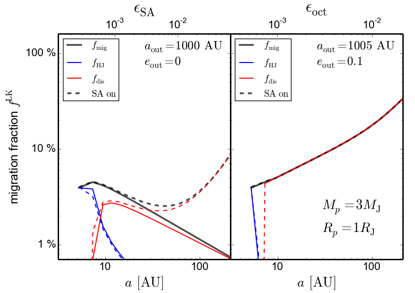
Figure 10: Same as Fig. 6 but with $a_{{\rm out}}=1000\ {\rm AU}$. Note log scale for $x$ axis.

Fig. 9 and 10 show the results of the analytic model with different values of $a_{{\rm out}}$ and ranges for $a_{{\rm in}}$.

References

- Abbott et al. (2016) Abbott B. P., et al., 2016, Phys. Rev. Lett., 116, 061102
- Abbott et al. (2017a) Abbott B. P., et al., 2017a, Phys. Rev. Lett., 118, 221101
- Abbott et al. (2017b) Abbott B. P., et al., 2017b, Phys. Rev. Lett., 119, 141101
- Anderson et al. (2016) Anderson K. R., Storch N. I., Lai D., 2016, MNRAS, 456, 3671
- Antognini (2015) Antognini J. M. O., 2015, MNRAS, 452, 3610
- Antognini et al. (2014) Antognini J. M., Shappee B. J., Thompson T. A., Amaro-Seoane P., 2014, MNRAS, 439, 1079
- Antonini & Perets (2012) Antonini F., Perets H. B., 2012, ApJ, 757, 27
- Antonini et al. (2014) Antonini F., Murray N., Mikkola S., 2014, ApJ, 781, 45
- Antonini et al. (2017) Antonini F., Toonen S., Hamers A. S., 2017, ApJ, 841, 77
- Askar et al. (2017) Askar A., Szkudlarek M., Gondek-Rosińska D., Giersz M., Bulik T., 2017, MNRAS, 464, L36
- Bartos et al. (2017) Bartos I., Kocsis B., Haiman Z., Márka S., 2017, ApJ, 835, 165
- Belczynski et al. (2016) Belczynski K., Repetto S., Holz D. E., O’Shaughnessy R., Bulik T., Berti E., Fryer C., Dominik M., 2016, ApJ, 819, 108
- Blaes et al. (2002) Blaes O., Lee M. H., Socrates A., 2002, ApJ, 578, 775
- Ćuk & Burns (2004) Ćuk M., Burns J. A., 2004, AJ, 128, 2518
- Eggleton & Kiseleva-Eggleton (2001) Eggleton P. P., Kiseleva-Eggleton L., 2001, ApJ, 562, 1012
- Fabrycky & Tremaine (2007) Fabrycky D., Tremaine S., 2007, ApJ, 669, 1298
- Ford et al. (2000) Ford E. B., Kozinsky B., Rasio F. A., 2000, ApJ, 535, 385
- Fragione & Kocsis (2018) Fragione G., Kocsis B., 2018, preprint, (arXiv:1806.02351)
- Fragione & Leigh (2018a) Fragione G., Leigh N., 2018a, MNRAS, 479, 3181
- Fragione & Leigh (2018b) Fragione G., Leigh N., 2018b, MNRAS, 480, 5160
- Frewen & Hansen (2016) Frewen S. F. N., Hansen B. M. S., 2016, MNRAS, 455, 1538
- Grishin et al. (2017) Grishin E., Perets H. B., Zenati Y., Michaely E., 2017, MNRAS, 466, 276
- Grishin et al. (2018) Grishin E., Lai D., Perets H. B., 2018, MNRAS, 474, 3547
- Haim & Katz (2018) Haim N., Katz B., 2018, preprint, (arXiv:1803.10249)
- Hamers (2017) Hamers A. S., 2017, ApJ Lett., 835, L24
- Hamers & Portegies Zwart (2016) Hamers A. S., Portegies Zwart S. F., 2016, MNRAS, 459, 2827
- Hamers et al. (2013) Hamers A. S., Pols O. R., Claeys J. S. W., Nelemans G., 2013, MNRAS, 430, 2262
- Hamers et al. (2018) Hamers A. S., Bar-Or B., Petrovich C., Antonini F., 2018, preprint, (arXiv:1805.10313)
- Hut (1981) Hut P., 1981, A&A, 99, 126
- Ivanov et al. (2005) Ivanov P. B., Polnarev A. G., Saha P., 2005, MNRAS, 358, 1361
- Katz & Dong (2012) Katz B., Dong S., 2012, preprint, (arXiv:1211.4584)
- Katz et al. (2011) Katz B., Dong S., Malhotra R., 2011, Physical Review Letters, 107, 181101
- Kinoshita & Nakai (2007) Kinoshita H., Nakai H., 2007, Celestial Mechanics and Dynamical Astronomy, 98, 67
- Kiseleva et al. (1998) Kiseleva L. G., Eggleton P. P., Mikkola S., 1998, MNRAS, 300, 292
- Knutson et al. (2014) Knutson H. A., et al., 2014, ApJ, 785, 126
- Kozai (1962) Kozai Y., 1962, AJ, 67, 591
- Li et al. (2014) Li G., Naoz S., Holman M., Loeb A., 2014, ApJ, 791, 86
- Lidov (1962) Lidov M. L., 1962, planss, 9, 719
- Lithwick & Naoz (2011) Lithwick Y., Naoz S., 2011, ApJ, 742, 94
- Liu & Lai (2017) Liu B., Lai D., 2017, ApJ Lett., 846, L11
- Liu & Lai (2018) Liu B., Lai D., 2018, preprint, (arXiv:1805.03202)
- Liu et al. (2015) Liu B., Muñoz D. J., Lai D., 2015, MNRAS, 447, 747
- Luo et al. (2016) Luo L., Katz B., Dong S., 2016, MNRAS, 458, 3060
- Michaely & Perets (2014) Michaely E., Perets H. B., 2014, ApJ, 794, 122
- Mikkola & Merritt (2006) Mikkola S., Merritt D., 2006, MNRAS, 372, 219
- Mikkola & Merritt (2008) Mikkola S., Merritt D., 2008, AJ, 135, 2398
- Muñoz et al. (2016) Muñoz D. J., Lai D., Liu B., 2016, MNRAS, 460, 1086
- Naoz (2016) Naoz S., 2016, ARA&A, 54, 441
- Naoz et al. (2011a) Naoz S., Farr W. M., Lithwick Y., Rasio F. A., Teyssandier J., 2011a, Nature, 473, 187
- Naoz et al. (2011b) Naoz S., Farr W. M., Lithwick Y., Rasio F. A., Teyssandier J., 2011b, Nature, 473, 187
- Naoz et al. (2012) Naoz S., Farr W. M., Rasio F. A., 2012, ApJ Lett., 754, L36
- Naoz et al. (2013a) Naoz S., Farr W. M., Lithwick Y., Rasio F. A., Teyssandier J., 2013a, MNRAS, 431, 2155
- Naoz et al. (2013b) Naoz S., Kocsis B., Loeb A., Yunes N., 2013b, ApJ, 773, 187
- Perets & Fabrycky (2009) Perets H. B., Fabrycky D. C., 2009, ApJ, 697, 1048
- Perets & Kratter (2012) Perets H. B., Kratter K. M., 2012, ApJ, 760, 99
- Perets & Naoz (2009) Perets H. B., Naoz S., 2009, ApJ Lett., 699, L17
- Peters (1964) Peters P. C., 1964, Physical Review, 136, 1224
- Petrovich (2015) Petrovich C., 2015, ApJ, 799, 27
- Petrovich & Tremaine (2016) Petrovich C., Tremaine S., 2016, ApJ, 829, 132
- Poincaré (1892) Poincaré H., 1892, Les methodes nouvelles de la mecanique celeste
- Raghavan et al. (2010) Raghavan D., et al., 2010, ApJ Suppl. Ser., 190, 1
- Randall & Xianyu (2018a) Randall L., Xianyu Z.-Z., 2018a, preprint, (arXiv:1802.05718)
- Randall & Xianyu (2018b) Randall L., Xianyu Z.-Z., 2018b, ApJ, 853, 93
- Rein & Liu (2012) Rein H., Liu S.-F., 2012, A&A, 537, A128
- Rein & Spiegel (2015) Rein H., Spiegel D. S., 2015, MNRAS, 446, 1424
- Rodriguez et al. (2018) Rodriguez C. L., Amaro-Seoane P., Chatterjee S., Rasio F. A., 2018, Phys. Rev. Lett., 120, 151101
- Silsbee & Tremaine (2017) Silsbee K., Tremaine S., 2017, ApJ, 836, 39
- Stephan et al. (2018) Stephan A. P., Naoz S., Gaudi B. S., 2018, preprint, (arXiv:1806.04145)
- Stone et al. (2017) Stone N. C., Metzger B. D., Haiman Z., 2017, MNRAS, 464, 946
- Tokovinin (2014) Tokovinin A., 2014, AJ, 147, 86
- Toonen et al. (2016) Toonen S., Hamers A., Portegies Zwart S., 2016, Computational Astrophysics and Cosmology, 3, 6
- Tremaine et al. (2009) Tremaine S., Touma J., Namouni F., 2009, AJ, 137, 3706
- Valtonen & Karttunen (2006) Valtonen M., Karttunen H., 2006, The Three-Body Problem
- Wen (2003) Wen L., 2003, ApJ, 598, 419
- Winn & Fabrycky (2015) Winn J. N., Fabrycky D. C., 2015, ARA&A, 53, 409
- Wright et al. (2011) Wright J. T., et al., 2011, PASP, 123, 412
- Wu & Murray (2003) Wu Y., Murray N., 2003, ApJ, 589, 605