Numerical aspect of large-scale electronic state calculation for flexible device material

Abstract

Numerical aspects of large-scale electronic state calculation are explored on flexible organic device materials. Physical theory, numerical method and real application studies are discussed in the context of application-algorithm-architecture co-design. An application study was carried out for disordered organic thin film. Participation ratio, a measure for the spatial extension of electronic wavefunction is focused on, since it is crucial for device property. A data scientific research is reported for a classification problem of disordered organic polymers, in which participation ratio is used as descriptor. These application studies indicate the potential need of purpose-specific solvers for internal eigenpairs.

1 Introduction

Large-scale quantum material simulation or electronic state calculation is one of the major fields in computational science with supercomputers. A central problem in this field is the generalized eigenvalue equation, in which an eigenvalue or eigenvector is the energy or the wavefunction of an electron, respectively. Although the de fact standard parallel solver library is ScaLAPACK SCALAPACK , these routines show severe limitations in parallel efficiency and several scalable solvers, such as ELPA ELPA-URL , ELPA2014 and EigenExa EigenExa-URL , EigenExa-PAPER , were developed recently. Among them, ELPA was developed in the tight collaboration between numerical researchers and material researchers in Europe. FHI-AIMS ; ELPA2014 Such a fruitful collaboration requires the co-design approach among application, algorithm and architecture, because an optimal algorithm is dependent both on problem and architecture. For example, a ELPA paper ELPA2014 discusses the benchmark of the calculation that obtains all the eigenvalues and a small fraction (10-50 %) of eigenvectors, since such calculations are typical among electronic state calculations.

The present paper reports large-scale electronic state calculations in the context of application-algorithm-architecture co-design. The target application is organic flexible device materials, and the application study contains (i) large single problem and (ii) many small problems in data scientific research for the classification of disordered materials. These researches lead us to a potential need for purpose-specific numerical solvers for internal eigenpairs. We believe that the present paper is a seed of the collaboration between numerical researcher and material researcher with the next-generation or (pre-)exascale supercomputers.

The present paper is organized as follows; Section  2 gives a brief overview of organic material. Physical theory and related numerical method of large-scale electronic state calculation appear in Sec. 3. The calculated results appear for organic thin film in Sec. 4.1 and for organic polymer in Sec. 4.2. The potential need for purpose-specific solvers is discussed in Sec. 4.3. Section 5 is devoted to summary and future outlook.

2 Organic materials

Organic semiconductor material is the foundation of flexible devices, such as flexible displays GELINCK-2004 , flexible solar cells XU-2018 , and human-friendly wearable electronics SEKITANI-2011 . Unlike inorganic semiconductors such as silicon, an organic semiconductor consists of small molecules or polymers which form solids with weak van der Waals interaction. An important industrial problem is to control the disorder of the atomic structure without an increase of the fabrication cost. The electronic property is highly anisotropic and is governed by the spatial extension of the characteristic electrons called $\pi$ electrons that lie, for example, on benzene rings. A fundamental issue is a conflicting demand on opt-electronic devices; An extended wavefuntion is preferable for conduction property, since an extended wavefunction can induce the electrical current easily. A localized wavefunction, by contrast, is preferable for optical property, since a localized wavefunction can strongly interact with light. The above conflicting demand should be a foundation of material design. Wavefunctions in disordered structures are localized, while wavefunctions in ideal crystalline (periodic) structures are extended throughout the whole system.

An investigation on these materials requires large-scale electronic state calculation in 10-100 nm scales, since complicated disordered structure is crucial for device properties. The investigation requires also a data scientific research with capacity computation, or simultaneous computation of many problems, because the real device property stem from the average among many disordered samples.

Here a crucial issue is to find a proper quantity that characterizes each disordered sample in the context of device property. In the present paper, the quantity is chosen to be participation ratio (PR) PARTICIPATION-RATIO1 , PARTICIPATION-RATIO2 , PARTICIPATION-RATIO3 , PARTICIPATION-RATIO4 , PARTICIPATION-RATIO5 , the spatial extension of electronic wavefunctions, since the spatial extension of wavefunctions governs the device property. The detailed explanation of PR will be given in the next section. Later in the present paper, PR will be used as descriptor in a data scientific research for classification.

3 Theory and numerical method

Numerical foundation of electronic state calculations is explained as the basics of the co-design approach. Details of the physical theory can be found in textbooks, such as Ref. MARTIN-TEXTBOOK .

3.1 Physical origin of matrix problem

The fundamental Schrödinger-type equation, a partial differential equation in real space $\bm{r}$, is written for an electronic wavefunction $\phi(\bm{r})$ as

$$\hat{H}\phi(\bm{r})=\lambda\phi(\bm{r})$$ (1)

with the Hamilton operator of

$$\hat{H}\equiv-\frac{\hbar^{2}}{2m}\Delta+V_{\rm eff}(\bm{r}).$$ (2)

Here, $\Delta$ is Laplacian, $m$ is the mass of electron and $\hbar$ is the Planck constant, a physical constant ($\hbar\approx 1.05^{-34}$Js). $V_{\rm eff}(\bm{r})$ is the effective potential, a scalar function. The normalization condition of

$$\int|\phi(\bm{r})|^{2}d\bm{r}=1$$ (3)

is imposed and stems from the fact that the sum of the weight distribution of one electron should be the unity. The function of $n(\bm{r})\equiv|\phi(\bm{r})|^{2}(\geq 0)$ is the weight distribution of the electron at the point of $\bm{r}$. The normalization condition of Eq. (3) can be expressed as

$$\int n(\bm{r})d\bm{r}=1.$$ (4)

An eigenvalue of $\lambda$ means the energy of an electron in the material and is called eigenenergy. The $k$-th eigenpair of $(\lambda_{k},\phi_{k}(\bm{r}))$ is defined for $k=1,2,..,M$ in the order of $\lambda_{1}\leq\lambda_{2}\leq\cdots\leq\lambda_{M}$. Each material has a specific integer of $k_{\rm HO}$ called highest occupied eigenenergy, and the eigenpairs for $k=1,2,...k_{\rm HO}$ are occupied by the electrons. A para-spin material with $N_{\rm elec}$ electrons, for example, gives the value of $k_{\rm HO}=N_{\rm elec}/2$, if $N_{\rm elec}$ is even. Semiconductor material has a finite energy gap between the $k_{\rm HO}$-th and $(k_{\rm HO}+1)$-th eigenenergies ($\lambda_{k_{\rm HO}+1}-\lambda_{k_{\rm HO}}>0$).

Now we consider, as a typical case, that $\phi(\bm{r})$ is expressed as a linear combination of given basis functions

$$\phi(\bm{r})=\sum_{j}^{M}v_{j}\chi_{j}(\bm{r}),$$ (5)

where $M$ is the number of the basis functions $\{\chi_{j}(\bm{r})\}$. The basis functions $\{\chi_{j}(\bm{r})\}$ are normalized to be

$$\int\chi^{\ast}_{j}(\bm{r})\chi_{j}(\bm{r})d\bm{r}=1.$$ (6)

A typical function is called atomic orbital and is localized near the position of an atomic nucleus. Since each basis function belongs to one atom, the basis index $i$ is equivalent to the composite indices of an atom index $I$ and an orbital index $\alpha$ ($i\equiv(I,\alpha)$). The orbital index $\alpha$ distinguishes the basis functions that belong to the same atom but different in their shape.

A generalized eigenvalue equation appears, when Eq (5) is substituted for Eq. (1);

$$A\bm{v}=\lambda B\bm{v}$$ (7)

with the $M\times M$ matrices of

$$A_{ij} \equiv \int\chi_{i}^{\ast}(\bm{r})\hat{H}\chi_{j}(\bm{r})d\bm{r}$$ (8)

$$B_{ij} \equiv \int\chi_{i}^{\ast}(\bm{r})\chi_{j}(\bm{r})d\bm{r}.$$ (9)

The matrices $A$ and $B$ are Hermitian. The matrix $B$ is positive definite and satisfies $B_{jj}=1$ and $|B_{ij}|<1$($i\neq j$). Hereafter we consider, as among many researches, that the basis functions are real and the matrices $A$ and $B$ are real-symmetric. The normalization condition of Eq. (3) is reduced to

$$\bm{v}^{\rm T}B\bm{v}=1,$$ (10)

which is called $B$-normalization. The present paper will discuss matrix data generated by our simulation software ELSES ELSES-URL , ELSES-2012 , an electronic-state calculation software with first-principles-based modeled (tight-binding) electronic-state theory. Sparsity of the matrices of $A_{ij}$ and $B_{ij}$ are explained briefly. As explained in the previous subsection, the indices $i$ and $j$ are the composite indices of the atom indices $I$ and $J$ and the orbital indices $\alpha$ and $\beta$, respectively ($i\equiv i(I,\alpha),j\equiv j(J,\beta))$). Therefore, an element of the matrices $A$ and $B$ is expressed by the four indices as $A_{I\alpha;J\beta}$ and $B_{I\alpha;J\beta}$, respectively. Since a matrix element value decreases quickly and monotonically as the function of the inter-atomic distance between the $I$-th and $J$-th atoms ($r_{IJ}$), a cutoff distance $r_{\rm cut}$ can be introduced. A matrix element, $A_{I\alpha;J\beta}$ or $B_{I\alpha;J\beta}$, is ignored, if $r_{IJ}>r_{\rm cut}$, which makes the matrices to be sparse.

3.2 Mulliken weight

This subsection introduces Mulliken weight MULLIKEN-CHARGE , a famous discretized representation for the weight distribution of $n(\bm{r})$. When the quantity of $q_{i}^{\rm(bas)}$ is defined as

$$q_{i}^{\rm(bas)}\equiv\sum_{j}v_{i}B_{ij}v_{j},$$ (11)

for $i=1,2,....,M$, it is called Mulliken weight at the $i$-th basis function. The normalization condition of Eq. (10) is reduced to

$$\sum_{i}q_{i}^{\rm(bas)}=1,$$ (12)

which is analogous to Eq. (4).

Since the basis index of $i$ is the composite indices of the atom index of $I$ and the orbital index of $\alpha$ ($i\equiv(I,\alpha)$), the Mulliken weight at the $I$-th atom is defined as

$$q^{\rm(atm)}_{I}\equiv\sum_{\alpha}q_{I,\alpha}^{\rm(bas)}$$ (13)

and satisfies

$$\sum_{I}^{\rm(atm)}q^{\rm(atm)}_{I}=1{.}$$ (14)

If each atom belongs to one molecule, the Mulliken weight at the $P$-th molecule is defined as

$$q^{\rm(mol)}_{P}\equiv\sum_{I}^{{\rm(atm)}\in P}q^{\rm(atm)}_{I},$$ (15)

where $\sum_{I}^{{\rm(atm)}\in P}$ is the summation among the atoms that belong to the $P$-th molecule. The sum is the unity;

$$\sum_{P}^{\rm(mol)}q^{\rm(mol)}_{P}=1.$$ (16)

In this paper, we will use the definition of $\bm{q}^{\rm(bas)}\equiv(q_{1}^{\rm(bas)},q_{2}^{\rm(bas)},...,q_{M}^{\rm(bas)})^{\rm T}$ and $\bm{q}^{\rm(mol)}\equiv(q_{1}^{\rm(mol)},q_{2}^{\rm(mol)},...,q_{\mu}^{\rm(mol)})^{\rm T}$, where $\mu$ is the number of the molecules in the system.

3.3 Participation ratio

This subsection introduces participation ratio (PR), as a measure of the spatial extension of wavefunctions $\phi(\bm{r})$ or how the wavefunction spreads in real space PARTICIPATION-RATIO1 , PARTICIPATION-RATIO2 , PARTICIPATION-RATIO3 , PARTICIPATION-RATIO4 . Since the spatial extension of wavefunction governs the electrical conductivity, PR was used with large-scale electronic state calculations, such as a research on the anomalous electrical conductivity in quasi crystals PARTICIPATION-RATIO5 .

In the continuum representation, PR is defined for a wavefunction $\phi(\bm{r})$ as

$$P^{\rm(cnt)(4)}(\phi)\equiv\left(\int|\phi(\bm{r})|^{4}d\bm{r}\right)^{-1}.$$ (17)

under the $L^{2}$-normalization of Eq. (3). For example, suppose $D$ is a closed area whose volume is $\Omega$ and $\phi$ is constant in $D$ as

$$\phi(\bm{r})=\left\{\begin{array}[]{ll}\frac{1}{\sqrt{\Omega}}&(\bm{r}\in D)\\ 0&(\rm{otherwise}).\end{array}\right.$$ (20)

Then the PR of $\phi$ gives the volume of the non-zero region of $\phi$

$$P^{\rm(cnt)(4)}(\phi)=\left(\frac{1}{\Omega^{2}}\int_{D}d\bm{r}\right)^{-1}=\Omega.$$ (21)

The above definition of PR can be expressed also by the weight distribution of $n(\bm{r})$ as

$$P^{\rm(cnt)(2)}(n)\equiv\left(\int|n(\bm{r})|^{2}d\bm{r}\right)^{-1}$$ (22)

under the normalization of Eq. (4).

PR for the eigenvector of $\bm{v}\equiv(v_{1},v_{2},....,v_{M})^{\rm T}$ in Eq. (7) can be also defined in a similar manner. The definition in the present paper is

$$P^{(4)}(\bm{v})\equiv\left(\sum_{j}{|v_{j}|^{4}}\right)^{-1}$$ (23)

under the $B$-normalization constraint of Eq. (10). For the discretized representation, PR indicates a measure of the number of non-zero elements, namely, how broadly the elements exist on the indices. For example, the case of $B=I$ and

$$\bm{v}\equiv\left(\frac{1}{\sqrt{3}},\frac{1}{\sqrt{3}},\frac{1}{\sqrt{3}},0,0,...,0\right)^{T},$$ (24)

the PR is

$$P^{(4)}=\left\{\sum_{j}|v_{j}|^{4}\right\}^{-1}=\left\{3\left(\frac{1}{\sqrt{3}}\right)^{4}\right\}^{-1}=3.$$ (25)

Another definition is the one for the Mulliken weight on basis function as

$$P^{(2)}(\bm{q}^{\rm(bas)})\equiv\left(\sum_{j}{|q_{j}^{\rm(bas)}|^{2}}\right)^{-1}$$ (26)

or the one for the Mulliken weight on molecules as

$$P^{(2)}(\bm{q}^{\rm(mol)})\equiv\left(\sum_{P}^{\rm(mol)}{|q_{P}^{\rm(mol)}|^{2}}\right)^{-1}.$$ (27)

The quantity of Eq.(27) is called ‘molecular PR’ in this paper and will appear later in this paper.

3.4 Sparsity of matrix data

According to the physical origin, the sparsity in matrix data of $A$ and $B$ is determined by the atomic structure of the simulated system. If a system contains independent (non-interacting) molecules, for example, the matrices of $A$ and $B$ are block diagonal and, each block stems from a molecule. The sparsity of the matrices is crucial for the efficiency of sparse-matrix solvers.A matrix data library of ‘ELSES matrix library’ ELSES-MATRIX-LIB was constructed, so as to enhance the collaboration between material and numerical researchers. The sparsity is different among the matrix data, as seen in Fig. 3 of Ref. K-EP , for example. Two examples are explained; The matrix data of ‘APF4686’ stems from an organic polymer system, poly-(9,9 dioctyl-fluorene), in a disordered structure with 2076 atoms ELSES-2012 , ELSES-2014 . The matrix size is $M=4686$ and the number of non-zero elements is $N_{\rm NZ}=53950$. The ratio of non-zero elements is $\gamma\equiv N_{\rm NZ}/M^{2}\approx 0.0025$. On the other hand, the matrix data of ‘AUNW9180’ stems from a disordered multishell gold nanowires with 1020 atoms HOSHI-2009-AUNW . The matrix size of is $M=9180$ and the number of non-zero elements is $N_{\rm NZ}=1783313$. The ratio of non-zero elements is $\gamma\equiv N_{\rm NZ}/M^{2}\approx 0.021$. It is noteworthy that ELSES matrix library has several features for the convenience of numerical researchers; (i) The matrix data files are recorded in the Matrix-Market format. MATRIX-MARKET (ii) Eigenvalues and PR values are stored as files, as well as the matrix data.

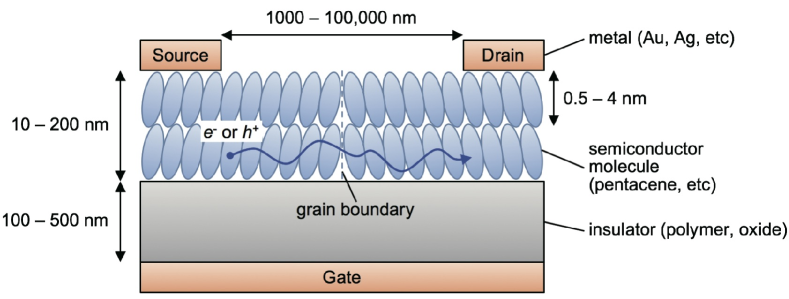
Figure 1: Schematic structure and typical scales of organic field-effect transistors. The electrical current is depicted as an arrow squiggle.

4 Result

The present section is devoted to the results of large-scale electronic state calculations of organic semiconductor materials. The present paper focuses on p-type semiconductor, in which the electrical current stems from a small number of wavefunctions that has the internal eigenenergies $\lambda_{k}$ near the highest occupied one $\lambda_{\rm HO}$ ($\lambda_{k}\leq\lambda_{\rm HO}$). Therefore, one should calculate only these internal eigenpairs.

We calculated thin film or two-dimensional condensed organic semiconductor molecules in disordered structures, which is a proto-typical system of organic field-effect transistors (OFETs) shown schematically in Fig. 1. OFETs consist of four layers: a gate electrode layer, an insulating layer, an organic semiconductor layer, and a source/drain electrode layer, typical scales of which are shown in Fig. 1. The details of Fig. 1 is explained in textbooks, like Ref. OFET-TEXTBOOK . In the OFETs, the electrical current flows on several atomic semiconductor layers on the interface region between the polycrystalline semiconductor and amorphous insulator layers. So we should investigate a thin film system with disordered structures.

The present calculated system is a thin film of pentacene molecules (C₂₂H₁₄). Pentacene is one of the most famous organic semiconductors. The present study is motivated by an experimental data of electron spin resonance (ESR) experiment for pentacene OFETs MATSUI-ESR-2010 ; MATSUI-ESR-2013 . The analysis of hyperfine interaction between hole carriers and protons in pentacene thin film in ESR spectra gives a molecular PR defined in Eq.(27) MATSUI-ESR-2010 . The molecular PR is denoted as $P$ hereafter. The experimental data indicates the appearance of ‘semi-localized’ wavefunction that is extended among a few tens of molecules $(P=O(10))$. Such semi-locality is crucial for the device performance.

The generalized eigenvalue problem was solved by the mini-application of EigenKernel IMACHI-JIT2016 , EIGENKERNEL-URL , EIGENKERNEL-2018 . EigenKernel is a middleware for the various solvers in ScaLAPACK, ELPA, and EigenExa and their hybrids. Although we have developed a massively parallel electronic state calculation method without eigenvalue problem ELSES-URL , ELSES-2012 , HOSHI2016SC16 , we still need eigenvalue solver, so as to obtain eigenpairs in the discussion of electronic property.

4.1 Large-scale calculation of thin film organic material

The calculated system is a thin-film (single molecular layer) system with an artificial two-dimensional periodic simulation cell. The simulation cell contains $N_{\rm mol}$=1800 molecules, and the matrix size of the generalized eigenvalue problem is $M=183600$. Thousands of molecules are required in the simulation cell, so as to observe a semi-localized state extended among tens of molecules ($N_{\rm mol}\gg O(10)$).

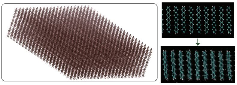
Figure 2: Preparation of disordered pentacene thin film sample. (a) The initial structure of a three-layered sample in the crystalline geometry. (b) The result of finite-temperature simulation.

The initial atomic structure of the disordered thin film sample was generated in classical molecular dynamics simulations by GROMACS GROMACS-URL , GROMACS with the generalized AMBER force field (GAFF) parameter set GAFF . The software and parameter set are standard for organic materials. The sample was prepared in the following stages; (I) A layered structure of pentacene in the crystalline geometry was prepared with three layers, shown in Fig. 2(a). (II) Several finite temperature simulations were carried out at the temperature of 300-1000 K for the dynamics in 0.1-100 ns, so as to generate a finite-temperature disordered structure, as shown in Fig. 2(b). In the simulation, only the middle layer in Fig. 2(a) was set to be mobile, and the upper and lower layers were set to be fixed, so as to impose the boundary condition on the middle layer. The temperature of the simulation should be distinguished from the experimental one, owing to the boundary condition and we have not yet compared the detailed results among different temperature and/or simulation time. A long-time (nano-second) dynamics is difficult for quantum simulation, owing to huge CPU time and we used the classical simulation. Classical simulations, however, do not treat electronic wavefunction, and the electronic state calculation is required for the disordered structure, so as to obtain wavefunctions. The total computational time of the classical molecular dynamics simulation is $T_{\rm comp}\approx$ 5 hours for a nano-second dynamics by six nodes of a Intel-Xeon-based Supercomputer at the Academic Center for Computing and Media Studies, Kyoto University. The time of the quantum simulation is $T_{\rm comp}\approx$ 6 hours by 36 nodes of a Intel-Xeon-based Supercomputer at the Institute for Solid State Physics, the University of Tokyo, when the ScaLAPACK solver was used. It is noteworthy that the computational time of the quantum simulation with a dense-matrix solver is proportional to $N_{\rm mol}^{3}$ and will be severe for a larger sample, while the time of the classical simulation is proportional to $N_{\rm mol}^{d}$ with $1\leq d\leq 2$.

Figure 3 shows a typical wavefunction with the molecular PR of $P\approx 35$, which agrees with the experimental observation of semi-localized wavefunction ($P=O(10)$). We should say, however, that the present simulation is the one for an isolated thin film system of pentacene layer and ignores the affects the neighboring layers, whereas the experimental result MATSUI-ESR-2010 ; MATSUI-ESR-2013 indicates the importance of the neighboring insulator layer shown in Fig. 1. Now the calculations are on going for the interface system including pentacene layer and insulator layers.

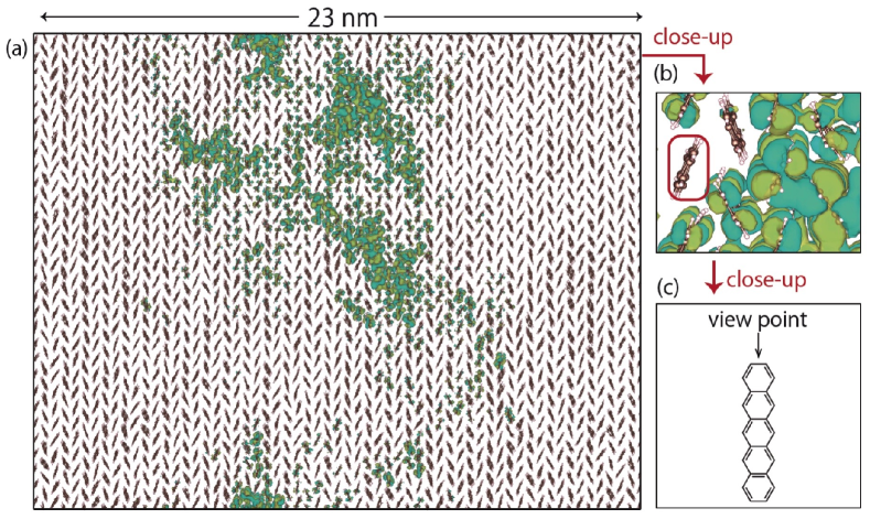
Figure 3: Example of semi-localized wavefunction that appears on a pentacene thin-film system. The wavefunction $\phi(\bm{r})$ has the eigenenergy of $\lambda\approx-0.15$eV, where the energy origin $(\lambda\equiv 0)$ is set to be the eigenenergy of the highest occupied wavefunction. The wavefunction of $\phi(\bm{r})$ is depicted as two iso-surfaces in the opposite signs ($\phi(\bm{r})=\pm C$, where $C$ is a positive constant). The two surfaces are painted by different colors. (a) The whole region of the periodic simulation cell. (b) A close-up of (a). (c) A picture of a single pentacene molecule with the view point of (b).

4.2 Data scientific research of organic polymers

This subsection gives a data scientific research with capacity computation, or simultaneous computation of many middle-size problems. The purpose of the research is how to characterize the disordered structure in the context of device property. In general, the spatial extension of wavefunction plays a crucial role on device property and is rigorously measured by PR for each wavefunction. Therefore a set of PR values among wavefunctions in a sample can be a candidate of the measure of the disorder for the sample. In other words, the set of PR values can be a descriptor that characterizes the sample.

The present paper focuses on a research on poly-(phenylene-ethynylene) (PPE)  TERAO-2013 , a typical conducting polymer. The paper measures the device property or the mobility for isolated polymers and found the importance of structural disorder. The first stage of theoretical research on disordered polymers is to define the descriptor of disordered polymers. The present paper proposes that the set of PR values can give a descriptor for a disordered sample.

Figure 4 shows a classification problem among $N_{\rm sample}=200$ disordered PPE polymer samples by the K-means clustering method, a typical classification algorithm. The structure of PPE polymers consists of 240 atoms, and a part is drawn in the inset of Fig. 4. A polymer sample consists of 20 benzene rings. The structural disorder was introduced in the relative rotation angles between adjacent benzene rings shown in $\theta$ in Fig. 4. The angles were set from the normal distribution with standard deviation of 20 or 60 degree. The samples were generated 100 times for each class (total $N_{\rm sample}=200$ samples). After the rotations, small fluctuations taken from the normal distribution with standard deviation of 0.01 Å were given to all the coordinates of all atoms to remove degeneracy. For each sample $(i=1,\dots,N_{\rm sample})$, the generalized eigenvalue problem of

$$H^{(i)}\bm{v}^{(i)}_{j}=\lambda^{(i)}_{j}S^{(i)}\bm{v}^{(i)}_{j}\ \ (j=1,\dots,M).$$ (28)

was solved numerically with the matrix size of $M=714$. Here, the list of PR value of all the eigenvectors

$$\bm{d}^{(i)}:=(P^{(4)}(\bm{v}^{(i)}_{1}),\dots,P^{(4)}(\bm{v}^{(i)}_{M})))^{T}$$ (29)

was used as the descriptor vector for the $i$-th sample.

The classification in the K-means clustering algorithm was carried out with the descriptor vectors of $\{\bm{d}^{(i)}\}_{i=1,\dots,M}$. The number of clusters was two. The classification result is shown in Fig. 4. Each sample is plotted on the plane by two statistical quantities with markers corresponding to the cluster labels given by the K-means algorithm. As a result, the two clusters perfectly matched to the structure classes. Namely, all the samples with adjacent rotation angles in standard deviation of 20 degree are clustered into one group, and all the samples with adjacent rotation angles in standard deviation of 60 degree are clustered into the other group. We should note the generality of PR as descriptor, since PR is calculated uniquely for any material without any preknowledge. The present result implies that the PR of wavefunctions can be a important quantity that bridges between disordered structure and device property. A more extensive study with principal component analysis is on going PCA-REPORT and will be reported elsewhere. It is noted that the present data scientific research is one among single polymer samples and a challenging future problem is the data scientific research for condensed polymer samples, as a foundation of device material research.

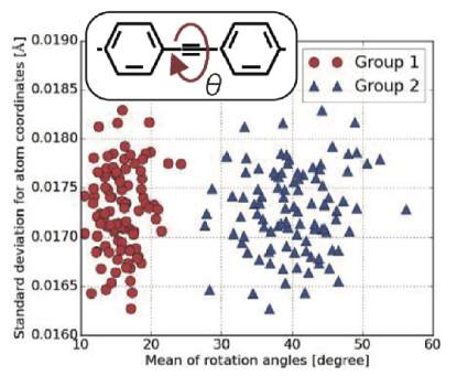
Figure 4: K-means clustering of polymer structures by their eigenvector participation ratios. Each structure is plotted by two statistical quantities. The x-axis is the mean of the rotation angles between adjacent benzene rings. The y-axis is the resulting standard deviation of the small fluctuation to the coordinates. Two markers, red circle and blue triangle, correspond to the two clusters labeled by the K-means algorithm.

4.3 Potential need of purpose-specific solvers

The application studies in the previous sections are carried out by the dense-matrix solver and implies the potential need of novel solvers. The largest matrix size in the present paper is $M=2\times 10^{5}$. In general, the computational cost of dense-matrix solvers is proportional to $M^{3}$ and a previous paper HOSHI2016SC16 reported that the dense-matrix solver solved a million dimensional generalized eigenvalue problem ($M=10^{6}$) by 1.5 hours with the whole system of the K computer. Since the above calculation indicates the practical upper limit of the dense-matrix solver, novel solvers are needed, at least, for a problem with $M\geq 10^{6}$.

Here we discusses the potential need of purpose-specific solvers suitable to the present problem. The need is the one for the solver of internal eigenpairs, like z-PARES Z-PARES ,Z-PARES-URL , FEAST FEAST ,FEAST-URL , the filtering method FILTERING , k-ep K-EP , K-EP-URL , because we would like to calculate only internal eigenpairs with the eigenenergies $\lambda_{k}$ near the highest occupied one $\lambda_{\rm HO}$ ($\lambda_{k}\leq\lambda_{\rm HO}$). Internal eigenpair solvers are desirable both for a solution of large problems, or a faster solution of middle-size problems. Application researchers, however, find sometimes the difficulty in choosing a solver, since the performance can be dependent on problem and machine. For example, the performance is dependent not only the matrix size $M$ but also the sparsity, when one uses a sparse-matrix solver. A possible remedy for the difficulty is to develop a ‘middleware’ that provides a universal interface for various solver routines, like EigenKernel.

5 Summary and future outlook

The present paper discusses the generalized eigenvalue problem in large-scale electronic state calculation for flexible organic device materials. The application studies were carried out for disordered organic thin film and polymer. The calculation of participation ratio is focused on, since it is a measure of the spatial extension of electronic wavefunctions and governs the device property. The present application research indicates the potential need of purpose-specific solvers with internal eigenpairs.

References

- (1) ScaLAPACK: http://www.netlib.org/scalapack/
- (2) ELPA: http://elpa.mpcdf.mpg.de/
- (3) Marek, A., Blum, V., Johanni, R., Havu, V., Lang, B., Auckenthaler, T., Heinecke, A., Bungartz, H. J. and Lederer, H., ‘The ELPA Library – Scalable Parallel Eigenvalue Solutions for Electronic Structure Theory and Computational Science’, J. Phys. Condens. Matter 26 (2014) 213201.
- (4) EigenExa: http://www.r-ccs.riken.jp/labs/lpnctrt/en/projects/eigenexa/
- (5) Imamura, T., Hirota, Y., Fukaya, T., Yamada, S., and Machida, M. ‘EigenExa: high performance dense eigensolver, present and future’, 8th International Workshop on Parallel Matrix Algorithms and Applications (PMAA14), Lugano, Switzerland, 2014.
- (6) Blum, V., Gehrke, R., Hanke, F., Havu, P., Havu, V., Ren, X., Reuter, K. and Scheffler, M.: Ab initio molecular simulations with numeric atom-centered orbitals, Computer Physics Communications 180 (2009) 2175-2196; https://aimsclub.fhi-berlin.mpg.de/
- (7) Gelinck, G. H., Huitema, H. E., van Veenendaal, E., Cantatore, E., Schrijnemakers, L., van der Putten, J. B., Geuns, T. C., Beenhakkers, M., Giesbers, J. B., Huisman, B. H., Meijer, E. J., Benito, E. M., Touwslager, F. J., Marsman, A. W., van Rens, B. J., de Leeuw, D. M., ‘Flexible active-matrix displays and shift registers based on solution-processed organic transistors’, Nat. Mater. 3 (2004) 106-110.
- (8) Xu, X., Fukuda, K., Karki, A., Park, S., Kimura, H., Jinno, H., Watanabe, N., Yamamoto, S., Shimomura, S., Kitazawa, D., Yokota, T., Umezu, S., Nguyen, T-Q., and Someya, T., ‘Thermally stable, highly efficient, ultraflexible organic photovoltaics’, PNAS 115 (2018) 4589-4594.
- (9) Sekitani, T., and Someya, T., ‘Human-friendly organic integrated circuits’, Mater. Today 14 (2011) 398-407.
- (10) Bell, R. J., and Dean, P., ‘Atomic vibrations in vitreous silica’, Disc. Faraday Soc. 50, (1970) 55-61.
- (11) Bell, R. J., ‘The dynamics of disordered lattices’, Rep. Prog. Phys. 35 (1972) 1315.
- (12) Thouless, D. J., ‘Electron in disordered systems and the theory of localization’, Phys. Rep. 13 (1974) 93-142.
- (13) Wegner, F., ‘Inverse Participation Ratio in 2 + Dimensions’, Z. Physik B 36 (1980) 209-214.
- (14) Fujiwara, T., Mitsui, T., and Yamamoto, S., ‘Scaling properties of wave functions and transport coefficients in quasicrystals’, Phys. Rev. B 53 (1996) R2910-R2913.
- (15) Martin, R. M., ‘Electronic Structure - Basic Theory and Practical Methods’, Cambridge University Press (2004).
- (16) ELSES: http://www.elses.jp
- (17) Hoshi, T., Yamamoto, S., Fujiwara, T., Sogabe, T. and Zhang, S.-L.: An order- electronic structure theory with generalized eigenvalue equations and its application to a ten-million-atom system, J. Phys. Condens. Matter 24 (2012) 165502.
- (18) Mulliken, R. S. ‘Electronic Population Analysis on LCAO-MO Molecular Wave Functions. I’, J. Chem. Phys. 23, (1955) 1833-1840.
- (19) ELSES matrix library: http://www.elses.jp/matrix/
- (20) Lee, D., Hoshi, T., Sogabe, T., Miyatake, Y., Zhang, S.-L., ‘Solution of the k-th eigenvalue problem in large-scale electronic structure calculations’, J. Comp. Phys. 371 (2018) 618-632.
- (21) Hoshi, T., Yamazaki, K., Akiyama, Y., ‘Novel linear algebraic theory and one-hundred-million-atom electronic structure calculation on the K computer’, JPS Conf. Proc. 1 (2014) 016004/1-4.
- (22) Hoshi, T., and Fujiwara, T., ‘Domain boundary formation in helical multishell gold nanowires’, J. Phys.: Condens. Matter 21 (2009), 272201/1-7.
- (23) Matrix Market: http://math.nist.gov/MatrixMarket/index.html
- (24) Imachi, H., Hoshi, T., ‘Hybrid numerical solvers for massively parallel eigenvalue computation and their benchmark with electronic structure calculations’, J. Inf. Process. 24 (2016) 164-172.
-
(25)
EigenKernel:
https://github.com/eigenkernel/ - (26) Tanaka, K., Imachi, H., Fukumoto, T., Fukaya, T., Yamamoto, Y., Hoshi, T., ‘EigenKernel - A middleware for parallel generalized eigenvalue solvers to attain high scalability and usability’, Preprint: http://arxiv.org/abs/1806.00741
- (27) Hoshi, T., Imachi, H., Kumahata, K., Terai, M., Miyamoto, K., Minami, K., and Shoji F.: Extremely scalable algorithm for 108-atom quantum material simulation on the full system of the K computer, Proceeding of 7th Workshop on Latest Advances in Scalable Algorithms for Large-Scale Systems (ScalA), held in conjunction with SC16: The International Conference for High Performance Computing, Networking, Storage and Analysis Salt Lake City, Utah November, 13-18 (2016) 33-40.
- (28) Bao, Z., Locklin, J., ‘Organic Field-Effect Transistors’, CRC Press (2007)
- (29) Matsui, H. , Mishchenko, A. S., and Hasegawa, T., Distribution of localized states from fine analysis of electron spin resonance spectra in organic transistors, Phys. Rev. Lett. 104, (2010) 056602/1-4.
- (30) Matsui, H., Mishchenko A. S. and Hasegawa, T. , Origin of shallow traps in organic transistors: dipole disorder at the semiconductor/insulator interface, The 68-th Annual Meeting of the Physical Society of Japan, 27pXP-4, Hiroshima University, 26-29., Mar. (2013)
- (31) GROMACS: http://www.gromacs.org/
- (32) Berendsen, H. J. C. . van der Spoel, D., van Drunen, R., GROMACS: A message-passing parallel molecular dynamics implementation, Comp. Phys. Comm. 91 (1995) 43-56.
- (33) Wang, J., Wolf, R. M., Caldwell, J. W., Kollmann, P. A., Case, D. A., Development and Testing of a General Amber Force Field, Comput. Chem. 25 (2004) 1157-1174.
- (34) Terao, J., Wadahama, A., Matono, A., Tada, T., Watanabe, S., Seki, S., Fujihara, T., Tsuji, Y., ‘Design principle for increasing charge mobility of -conjugated polymers using regularly localized molecular orbitals’, Nat. Commun. 4 (2013) 1691.
- (35) Hoshi, T., Imachi, H., Oohira, K., Abe, Y., Hukushima, K., ‘Principal component analysis with electronic wavefunctions for exploration of organic polymer device materials’, International Meeting on High-Dimensional Data-Driven Science (HD3-2017), Kyoto, Japan, 10-13, Sep. 2017.
- (36) Sakurai, T., Sugiura, H., A projection method for generalized eigenvalue problems using numerical integration, J. Comput. Appl. Math. 159(1) (2003) 119-128.
- (37) z-PARES: http://zpares.cs.tsukuba.ac.jp/
- (38) Polizzi, E., Density-matrix-based algorithm for solving eigenvalue problems, Phys. Rev. B 79 (2009) 115112/1-6.
- (39) FEAST: http://www.feast-solver.org/
- (40) Li, R., Xi, Y., Vecharynski, E., Yang, C., Saad, Y., A thick-restart Lanczos algorithm with polynomial filtering for Hermitian eigenvalue problems, SIAM J. Sci. Comput. 38(4) (2016) A2512-A2534.
- (41) k-ep: https://github.com/lee-djl/k-ep