Mass-spring-damper Networks for
Distributed Optimization in Non-Euclidean Spaces

Abstract

We consider the problem of minimizing the sum of non-smooth convex functions in non-Euclidean spaces, e.g., probability simplex, via only local computation and communication on an undirected graph. We propose two algorithms motivated by mass-spring-damper dynamics. The first algorithm uses an explicit update that computes subgradients and Bregman projections only, and matches the convergence behavior of centralized mirror descent. The second algorithm uses an implicit update that solves a penalized subproblem at each iteration, and achieves the iteration complexity of $\mathcal{O}(1/K)$. The results are also demonstrated via numerical examples.

, ,

1 Introduction

Given a connected graph, distributed optimization aims to optimize the sum of locally accessible cost functions via local computation and communication [Bertsekas and Tsitsiklis, 1989, Boyd et al., 2011]. Distributed optimization has a variety of engineering applications, such as formation control [Mesbahi and Egerstedt, 2010], distributed tracking and localization [Li et al., 2002], distributed estimation [Açıkmeşe et al., 2014, Lesser et al., 2012] and averaging [Xiao et al., 2007]. Due to such wide range of applications, distributed optimization has been an active area of research during the past two decades. Numerous distributed optimization algorithms have been developed, both in continuous time  [Wang and Elia, 2010, Wang and Elia, 2011, Gharesifard and Cortés, 2014, Kia et al., 2015, Qiu et al., 2016, Zeng et al., 2017, Yang et al., 2017, Hatanaka et al., 2018] and discrete time domains [Nedic and Ozdaglar, 2009, Nedic et al., 2010, Boyd et al., 2011, Wei and Ozdaglar, 2012, Meng et al., 2015]. The common feature of these algorithms revolves around sutiable generalization of centralized optimization algorithms to distributed scenarios.

Recently, there has been a growing interest in distributed optimization in non-Euclidean spaces, where the design variable is typically a probability distribution [Dekel et al., 2012, Levine et al., 2016, Gholami et al., 2016, Yahya et al., 2017]. In order to effectively exploit the structure of such non-Euclidean geometries, several attempts have been made to generalize distributed optimization algorithms from Euclidean to non-Euclidean setting. In particular, the distributed mirror descent method [Raginsky and Bouvrie, 2012, Li et al., 2016, Yuan et al., 2018, Wang et al., 2018, Doan et al., 2019] generalizes the distributed subgradient method [Nedic and Ozdaglar, 2009]; the distributed dual averaging algorithm [Duchi et al., 2012] generalizes projected distributed subgradient method [Nedic et al., 2010]; the Bregman parallel direction method of multipliers (BPDMM) [Yu et al., 2018] generalizes the proximal distributed alternating direction method of multipliers (ADMM) [Meng et al., 2015]. Compared with their counterparts in Euclidean cases [Nedic and Ozdaglar, 2009, Nedic et al., 2010, Meng et al., 2015], the key feature of these algorithms is to use a Bregman divergence instead of a quadratic function as the distance generating function, leading to an improved complexity bound of $\mathcal{O}(n/\ln n)$ [Wang and Banerjee, 2014, Yu et al., 2018] where $n$ represents the dimension of the problem instance.

However, there are still open questions along this line of research. In continuous time domain, compared with distributed Euclidean case [Wang and Elia, 2010, Wang and Elia, 2011, Gharesifard and Cortés, 2014, Kia et al., 2015, Qiu et al., 2016, Zeng et al., 2017, Yang et al., 2017] and centralized non-Euclidean case [Krichene et al., 2015, Wibisono et al., 2016], the ordinary differential equations (ODE) for distributed non-Euclidean optimization have attracted much less attention. In particular, it is unclear, to the best of our knowledge, whether the ODE setup in [Wang and Elia, 2010] and [Raginsky and Bouvrie, 2012] can be jointly utilized to design novel distributed optimization algorithms. In discrete time domain, although BPDMM [Yu et al., 2018] provides an extension to the proximal distributed ADMM [Meng et al., 2015], it requires a computationally expensive mirror averaging step. Moreover, like other algorithms based on ADMM [Wei and Ozdaglar, 2012, Meng et al., 2015, Yu et al., 2018], BPDMM uses implicit discretization, which requires solving an optimization problem at each iteration. As such, it remains unclear why explicit discretization, which only computes subgradients [Duchi et al., 2012, Li et al., 2016, Doan et al., 2019], cannot achieve similar convergence properties.

Figure 1: An example of mass-spring-damper network.

Motivated by these questions, as well as the connections between algorithm design and physics [Alvarez, 2000, Alvarez et al., 2002, Wibisono et al., 2016], we propose two novel algorithms for non-Euclidean distributed optimization with non-smooth convex objective functions over undirected graphs. Our algorithm is based on a mass-spring-damper network model (see Figure 1 for an illustration). In particular, we first propose a novel continuous time mass-spring-damper dynamics based on Bregman divergence type kinetic energy for distributed optimization. Using an explicit discretization, we show that discrete time mass-spring-damper dynamics matches the convergence behavior of centralized mirror descent. Further, if an implicit dicretization is used, such convergence can be improved to achieve $\mathcal{O}(1/K)$ iteration complexity. Finally, we demonstrate our results with numerical experiments.

Our results extend the existing literature as follows: 1) our continuous time model generalizes the second order ODE model of Euclidean cases [Wang and Elia, 2010] and the first order mirror descent ODE model of non-Euclidean cases [Raginsky and Bouvrie, 2012] by combining their attractive features; 2) our discrete time algorithms not only provide a novel extension to distributed mirror descent, but also generalize the proximal function used in distributed ADMM [Meng et al., 2015] from quadratic functions to a Bregman divergence. Such a generalization is empirically demonstrated to have faster convergence than subgradient based algorithms [Duchi et al., 2012, Li et al., 2016, Doan et al., 2019]; it also achieves the same iteration complexity and convergence properties as BPDMM [Yu et al., 2018] with a much more efficient implementation.

The rest of the paper is organized as follows. §2 provides necessary backgrounds in graph theory and convex analysis. §3 first introduces continuous time mass-spring-damper dynamics for distributed optimization, then establishes its convergence in discrete time using different discretization schemes. §4 compares our algorithms against existing methods via numerical examples. In §5 concluding remarks and comments on future research directions are provided.

2 Notation and Preliminaries

Let $\mathbb{N}$ denote the positive integers, $\mathbb{R}$ ($\mathbb{R}_{+}$) denote the (non-negative) real numbers, and $\mathbb{R}^{n}$ denote the $n$-dimensional real Euclidean space. We use $\cdot^{\top}$ to designate matrix (vector) transpose; $\langle u,v\rangle=u^{\top}v$ denotes the inner product of two vectors, and $\left\lVert\cdot\right\rVert_{2}$ is the $l_{2}$ norm, i.e., $\left\lVert v\right\rVert_{2}=\sqrt{\langle v,v\rangle}$ for $v\in\mathbb{R}^{n}$. Let $\mathop{\bf diag}(v)\in\mathbb{R}^{n\times n}$ denote the diagonal matrix whose diagonal elements are given by vector $v\in\mathbb{R}^{n}$; $\otimes$ designates the Kronecker product. Lastly, $I_{n}\in\mathbb{R}^{n\times n}$ denotes the identity matrix and $\mathbf{1}_{n}\in\mathbb{R}^{n}$ the vector of all $1$’s.

2.1 Graph theory

An undirected graph $\mathcal{G}=(\mathcal{V},\mathcal{E})$ consists of a node set $\mathcal{V}$ and an edge set $\mathcal{E}$, where an edge is a pair of distinct nodes in $\mathcal{V}$. The number of nodes and edges in the graph are denoted by $|\mathcal{V}|$ and $|\mathcal{E}|$, respectively. Denote by $\{ij\}$ an edge between nodes $i$ and $j$. For an arbitrary orientation on $\mathcal{G}$, i.e., each edge has a head and a tail, the $|\mathcal{V}|\times|\mathcal{E}|$ incidence matrix is denoted by $E(\mathcal{G})$. The columns of $E(\mathcal{G})$ are indexed by the edge set $\mathcal{E}$, and the entry on their $i$-th row takes the value “$1$” if node $i$ is the head of the corresponding edge and “$-1$” if it is its tail, and zero otherwise. When the graph is connected, the nullspace of $E(\mathcal{G})^{\top}$ is spanned by $\mathbf{1}_{|\mathcal{V}|}$ [Mesbahi and Egerstedt, 2010, Theorem 2.8].

2.2 Convex analysis

We say that $g$ is a subgradient of the convex function $f:\mathbb{R}^{n}\to\mathbb{R}$ at $x$ if [Rockafellar, 1970, Thm 23.2],

$$f(x^{\prime})-f(x)\geq\langle x^{\prime}-x,g\rangle,\enskip\forall x^{\prime}.$$ (1)

We denote by $\partial f(x)$ the set of subgradients of $f$ at $x$. Let $\delta_{\mathcal{X}}$ be the indicator function of a closed convex set $\mathcal{X}$, i.e., $\delta_{\mathcal{X}}(x)=0$ if $x\in\mathcal{X}$ and $+\infty$ otherwise. Then

$$\partial\delta_{\mathcal{X}}(x)=N_{\mathcal{X}}(x)=\{g|\langle g,x^{\prime}-x\rangle\leq 0,\forall x^{\prime}\in\mathcal{X}\}.$$ (2)

If $\psi$ is convex and continuously differentiable, then the Bregman divergence from $x^{\prime}$ to $x$ associated with $\psi$ is given by [Censor and Lent, 1981]

$$B_{\psi}(x^{\prime},x)=\psi(x^{\prime})-\psi(x)-\langle\nabla\psi(x),x^{\prime}-x\rangle.$$ (3)

Using (3) one can verify that for any $x,x^{+},x^{\prime}$,

$$B_{\psi}(x^{\prime},x^{+})-B_{\psi}(x^{\prime},x)-B_{\psi}(x^{+},x)$$ (4)

$$= \langle\nabla\psi(x^{+})-\nabla\psi(x),x^{\prime}-x^{+}\rangle.$$

Due to the convexity of $\psi$, $B_{\psi}(x^{\prime},x)$ is always non-negative. If $\psi$ is $1$-strongly convex, i.e., $\psi-\frac{1}{2}\left\lVert\cdot\right\rVert_{2}^{2}$ is convex, then using (1) we can show that $B_{\psi}(x^{\prime},x)\geq\frac{1}{2}\left\lVert x^{\prime}-x\right\rVert_{2}^{2}$.

3 Mass-spring-damper network dynamics for distributed optimization

In this section, we propose a mass-spring-damper dynamics (MSD) for the distributed optimization problem (P), leading to algorithms (MSD-ex) and (MSD-im) using explicit and, respectively, implicit discretization. We then establish their convergence properties in Theorem 1 and Theorem 2.

We consider the distributed optimization problem over the graph $\mathcal{G}=(\mathcal{V},\mathcal{E})$ of the following form,

$$\begin{array}[]{ll}\underset{x}{\mbox{minimize}}&f(x)=\sum\limits_{i\in\mathcal{V}}f_{i}(x_{i})\\ \mbox{subject to}&E_{s}(\mathcal{G})^{\top}x=0,\enskip x\in\mathcal{X}=\mathcal{X}_{0}^{|\mathcal{V}|},\end{array}$$ (P)

where $x=[x_{1}^{\top},\ldots,x_{|\mathcal{V}|}^{\top}]^{\top}$, $x_{i}\in\mathbb{R}^{n}$ for all $i\in\mathcal{V}$; $\mathcal{X}_{0}^{|\mathcal{V}|}$ is the Cartesian product of $|\mathcal{V}|$ copies of a closed convex set $\mathcal{X}_{0}\subset\mathbb{R}^{n}$; $f_{i}:\mathcal{X}_{0}\to\mathbb{R}$ is a cost function available to node $i$ only; matrix $E_{s}(\mathcal{G})$ is defined as

$$E_{s}(\mathcal{G})=(E(\mathcal{G})\mathop{\bf diag}(\sqrt{s}))\otimes I_{n},$$ (5)

where $\sqrt{s}$ is the element-wise square root of $s\in\mathbb{R}^{|\mathcal{E}|}$.

To solve problem (P), we propose the following mass-spring-damper dynamics,

$$\frac{d}{dt}\nabla\psi(x(t)) =-L_{d}(\mathcal{G})x(t)-E_{s}(\mathcal{G})u(t)-g(t)$$ (MSD)

$$\frac{d}{dt}u(t) =E_{s}(\mathcal{G})^{\top}x(t),$$

where $\psi(x)=\sum_{i\in\mathcal{V}}\psi_{0}(x_{i})$ with $\psi_{0}$ being a continuously differentiable convex function over $\mathcal{X}_{0}$, $g(t)=[g_{1}(t)^{\top},\ldots,g_{|\mathcal{V}|}^{\top}]^{\top}$ with $g_{i}(t)\in\partial f_{i}(x_{i}(t))$ for all $i\in\mathcal{V}$, and finally the weighted Laplacian is given by

$$L_{d}(\mathcal{G})=(E(\mathcal{G})\mathop{\bf diag}(d)E(\mathcal{G})^{\top})\otimes I_{n}.$$ (6)

Dynamics in (MSD) can be interpreted as a mass-spring-dynamic network as follows. Each node $i$ in $\mathcal{V}$ denotes a mass with velocity $x_{i}(t)$ experiencing external force $g_{i}(t)$; each edge denotes a spring with a spring constant $s_{\{ij\}}$ and damper with a damping constant $d_{\{ij\}}$, together connecting node $i$ and $j$; see Figure 1 for an illustration. If $\psi_{0}=\frac{m}{2}\left\lVert\cdot\right\rVert_{2}^{2}$, then (MSD) describes the Newton’s second law of such mass-spring-damper network, which is also analyzed in [Wang and Elia, 2010, Gharesifard and Cortés, 2014, Hatanaka et al., 2018]. Here we use a more general choice of $\psi_{0}$ to capture non-quadratic kinetic energy function used in Bregman Lagrangian dynamics [Wibisono et al., 2016].

We now group our assumptions on (P) and (MSD) under Assumption 1.

Assumption 1.

1. $\mathcal{G}=(\mathcal{V},\mathcal{E})$ is undirected and connected. Edge weights $s,d\in\mathbb{R}^{|\mathcal{E}|}$ are element-wise strictly positive. Let $\frac{1}{\gamma}=\max\{\alpha|\,\alpha s-d\leq 0\}$ and $\lambda$ be the largest eigenvalue of $L_{d}(\mathcal{G})$.

2. $\mathcal{X}_{0}\subset\mathbb{R}^{n}$ is a closed convex set, $\psi_{0}:\mathcal{X}_{0}\to\mathbb{R}$ is continuously differentiable and $1$-strongly convex, i.e., $\psi_{0}-\frac{1}{2}\left\lVert\cdot\right\rVert_{2}^{2}$ is convex.

3. $f_{i}:\mathcal{X}_{0}\to\mathbb{R}$ is proper closed convex function for all $i\in\mathcal{V}$. There exists $x^{\star},u^{\star},g^{\star}\in\partial f(x^{\star})$ such that

   $$E_{s}(\mathcal{G})^{\top}x^{\star} =0,\enskip x^{\star}\in\mathcal{X},$$ (7a)

   $$-g^{\star}-E_{s}(\mathcal{G})u^{\star} \in N_{\mathcal{X}}(x^{\star}).$$ (7b)

Remark 1.

Examples of $\mathcal{X}_{0}$ and $\psi_{0}$ that satisfy Assumption 1 include: 1) $\mathcal{X}_{0}=\mathbb{R}^{n}$ and $\psi_{0}(y)=\frac{1}{2}\left\lVert y\right\rVert_{2}^{2}$; 2) $\mathcal{X}_{0}$ is the probability simplex and $\psi_{0}(y)=\sum_{i=1}^{n}y[i]\ln y[i]$ for all $y\in\mathcal{X}_{0}$, known as the negative entropy function. See [Bubeck et al., 2015, Sec. 4.3] for further discussion.

Note that conditions in (7a) and (7b) ensure primal feasibility and, respectively, stationary condition of (P).

We first make the following observation on (MSD).

Lemma 1.

Suppose that Assumption 1 holds and there exists a trajectory $(x(t),u(t))$ for $t\in[0,\infty)$ generated by (MSD). Then

$$\ell(\overline{x}(T))-\ell(x^{\star})+\frac{1}{2}\langle L_{d}(\mathcal{G})\overline{x}(T),\overline{x}(T)\rangle\leq\frac{V(x(0),u(0))}{T},$$ (8)

for all $T>0$, where $\overline{x}(T)=\frac{1}{T}\int_{0}^{T}x(t)dt$, and

$$V(x,u)= B_{\psi}(x^{\star},x)+\frac{1}{2}\left\lVert u-u^{\star}\right\rVert_{2}^{2},$$ (9a)

$$\ell(x)= f(x)+\langle E_{s}(\mathcal{G})u^{\star},x\rangle.$$ (9b)

Proof Using the chain rule we can show that,

$$\frac{d}{dt}V(x,u)= -\langle\frac{d}{dt}\nabla\psi(x),x^{\star}-x\rangle+\langle\frac{d}{dt}u,u-u^{\star}\rangle$$ (10)

$$= \langle L_{d}(\mathcal{G})x+E_{s}(\mathcal{G})u^{\star}+g,x^{\star}-x\rangle$$

$$\leq \textstyle\ell(x^{\star})-\ell(x)-\frac{1}{2}\langle L_{d}(\mathcal{G})x,x\rangle,$$

for all $t$, where the last step is due to (1) and the assumption that $g(t)\in\partial f(x(t))$. Integrating on both sides from $t=0$ to $t=T$ we have

$$\int_{0}^{t}\ell(x(t))-\ell(x^{\star})+\frac{1}{2}\langle L_{d}(\mathcal{G})x(t),x(t)\rangle dt$$

$$\leq V(x(0),u(0))-V(x(T),u(T)).$$

Notice that, by construction, $V(x(T),u(T))$ is non-negative and $\ell(x)+\frac{1}{2}\langle L_{d}(\mathcal{G})x,x\rangle$ is convex. Therefore we can drop the last term on the right hand side. The rest of the proof is an application of Jensen’s inequality $\ell(\overline{x}(T))\leq\int_{0}^{T}\ell(x(\tau))d\tau$.∎ Lemma 1 provides a $\mathcal{O}(1/T)$ bound on the running duality gap [He and Yuan, 2012, Meng et al., 2015] and the disagreement on edges of the graph along any solution trajectory of (MSD). Although such a bound hinges on the existence of such a trajectory, requiring a separate existence proof in general, it does suggest that a similar property might hold for a discretization of (MSD), where the existence of a trajectory is easier to establish. In the following, we aim to show the validity of this intuition.

Consider the following discretization of (MSD),

$$\nabla\psi(x^{k+1})-\nabla\psi(x^{k})= -\alpha^{k}(L_{d}(\mathcal{G})x^{k}+E_{s}(\mathcal{G})u^{k}+g^{k})$$ (11)

$$u^{k+1}-u^{k}= \alpha^{k}E_{s}(\mathcal{G})^{\top}x^{k+1},$$

which is an explicit discretization combined with a Gauss-Seidel pass from $x$-update to $u$-update.

Using [Rockafellar, 1970, Thm 23.5], we can rewrite the $x$-update in (11) as,

$$x^{k+1}= \underset{x\in\mathcal{X}}{\mathop{\rm argmin}}\,\langle-\nabla\psi(x^{k})+\alpha^{k}(w^{k}+g^{k}),x\rangle+\psi(x)$$ (12)

$$= \underset{x\in\mathcal{X}}{\mathop{\rm argmin}}\,\alpha^{k}\langle g^{k}+w^{k},x\rangle+B_{\psi}(x,x^{k}),$$

where $w^{k}=L_{d}(\mathcal{G})x^{k}+E_{d}(\mathcal{G})u^{k}$. Therefore, a trajectory that satisfies (11) for all $k\in\mathbb{N}$ can be computed iteratively as,

$$w^{k}= L_{d}(\mathcal{G})x^{k}+E_{s}(\mathcal{G})u^{k}$$ (MSD-ex)

$$x^{k+1}= \underset{x\in\mathcal{X}}{\mathop{\rm argmin}}\,\,\alpha^{k}\langle g^{k}+w^{k},x\rangle+B_{\psi}(x,x^{k})$$

$$u^{k+1}= u^{k}+\alpha^{k}E_{s}(\mathcal{G})^{\top}x^{k+1},$$

where $g^{k}\in\partial f(x^{k})$, $\psi(x)=\sum_{i\in\mathcal{V}}\psi_{0}(x_{i})$.

To prove the convergence of (MSD-ex), we will use the following property of Bregman divergence.

Lemma 2.

Suppose Assumption 1 holds. Given a proper closed convex function $\phi:\mathcal{X}\to\mathbb{R}$, if $x^{+}=\mathop{\rm argmin}_{y\in\mathcal{X}}\,\,\phi(y)+B_{\psi}(y,x)$ for some $x\in\mathcal{X}$, then for any $x^{\prime}\in\mathcal{X}$,

$$B_{\psi}(x^{\prime},x^{+})-B_{\psi}(x^{\prime},x)$$

$$\leq -\frac{1}{2}\left\lVert x^{+}-x\right\rVert_{2}^{2}+\phi(x^{\prime})-\phi(x^{+}).$$

Proof Using Theorem 27.4 in [Rockafellar, 1970], we know that $x^{+}=\mathop{\rm argmin}_{y\in\mathcal{X}}\,\,\phi(y)+B_{\psi}(y,x)$ if and only if there exists $g\in\partial\phi(x^{+})$ such that

$$0\leq\langle g+\nabla\psi(x^{+})-\nabla\psi(x),x^{\prime}-x^{+}\rangle,$$ (13)

for all $x^{\prime}\in\mathcal{X}$. From (1), $\langle g,x^{\prime}-x^{+}\rangle\leq\phi(x^{\prime})-\phi(x^{+})$. Substitute this and (4) into (13) we have

$$B_{\psi}(x^{\prime},x^{+})-B_{\psi}(x^{\prime},x)\leq-B_{\psi}(x^{+},x)+\phi(x^{\prime})-\phi(x^{+}).$$

Finally, from Assumption 1 we know that $\psi-\frac{1}{2}\left\lVert\cdot\right\rVert_{2}^{2}$ is convex. Using (1) and (3) we can show that $B_{\psi}(x^{+},x)\geq\frac{1}{2}\left\lVert x^{+}-x\right\rVert_{2}^{2}$, which completes the proof. ∎ In our subsequent analysis, we will use the following inequality: if $\lambda$ is the largest eigenvalue of $L_{d}(\mathcal{G})$, then

$$-\langle L_{d}(\mathcal{G})x,x^{+}\rangle$$ (14)

$$\leq \frac{\lambda}{2}\left\lVert x^{+}-x\right\rVert_{2}^{2}-\frac{1}{2}\langle L_{d}(\mathcal{G})x,x\rangle-\frac{1}{2}\langle L_{d}(\mathcal{G})x^{+},x^{+}\rangle,$$

for all $x,x^{+}$; this is due to the fact that $\frac{1}{2}\langle L_{d}(\mathcal{G})(x^{+}-x),x^{+}-x\rangle\leq\frac{\lambda}{2}\left\lVert x^{+}-x\right\rVert_{2}^{2}$.

With these supporting inequalities, we are now ready to establish the convergence of (MSD-ex), which is our first main result.

Theorem 1.

Suppose that Assumptions 1 holds. If $0<\alpha^{k}\leq\min\{\frac{1}{2\lambda},\frac{1}{\gamma}\}$ for all $k\in\mathbb{N}$ and $\left\lVert g+E_{s}(\mathcal{G})u^{\star}\right\rVert_{2}\leq G$ for any $g\in\partial f(x)$ where $x\in\mathcal{X}$, then along the trajectories generated by algorithm (MSD-ex),

$$\ell(\overline{x}^{K})-\ell(x^{\star})+\frac{1}{2}\langle L_{d}(\mathcal{G})\overline{x}^{K},\overline{x}^{K}\rangle$$

$$\leq \frac{V(x^{1},u^{1})+G^{2}\sum_{k=1}^{K}(\alpha^{k})^{2}}{\sum_{k=1}^{K}\alpha^{k}},$$

where $\overline{x}^{K}=\frac{1}{\sum_{k=1}^{K}\alpha^{k}}\sum_{k=1}^{K}\alpha^{k}x^{k}$, $V(x,u)$ and $\ell(x)$ are defined as in (9).

Proof Applying Lemma 2 to the $x$-update in (MSD-ex) we have,

$$B_{\psi}(x^{\star},x^{k+1})-B_{\psi}(x^{\star},x^{k})$$ (15)

$$\leq \textstyle-\frac{1}{2}\left\lVert x^{k+1}-x^{k}\right\rVert_{2}^{2}+\alpha^{k}\langle g^{k}+E_{s}(\mathcal{G})u^{k},x^{\star}-x^{k+1}\rangle$$

$$-\alpha^{k}\langle L_{d}(\mathcal{G})x^{k},x^{k+1}\rangle.$$

In addition, applying (4) to function $\frac{1}{2}\left\lVert\cdot\right\rVert_{2}^{2}$ and using the $u$-update in (MSD-ex), we obtain

$$\textstyle\frac{1}{2}\left\lVert u^{k+1}-u^{\star}\right\rVert^{2}-\frac{1}{2}\left\lVert u^{k}-u^{\star}\right\rVert^{2}$$ (16)

$$= \textstyle\frac{(\alpha^{k})^{2}}{2}\langle L_{s}(\mathcal{G})x^{k+1},x^{k+1}\rangle$$

$$+\alpha^{k}\langle u^{k}-u^{\star},E_{s}(\mathcal{G})^{\top}(x^{k+1}-x^{\star})\rangle,$$

where we have used (7a) and $L_{s}(\mathcal{G})=E_{s}(\mathcal{G})E_{s}(\mathcal{G})^{\top}$. Adding (16) to (15) and using (14), we can show that,

$$V(x^{k+1},u^{k+1})-V(x^{k},u^{k})$$ (17)

$$\leq \textstyle\alpha^{k}\langle h^{k},x^{\star}-x^{k+1}\rangle-\frac{\alpha^{k}}{2}\langle L_{d}(\mathcal{G})x^{k},x^{k}\rangle$$

$$\textstyle-\frac{1-\alpha^{k}\lambda}{2}\left\lVert x^{k+1}-x^{k}\right\rVert_{2}^{2}-\frac{\alpha^{k}}{2}\langle L_{c}(\mathcal{G})x^{k+1},x^{k+1}\rangle,$$

where $c=d-\alpha^{k}s$ and $h^{k}=g^{k}+E_{s}(\mathcal{G})u^{\star}$. Observe that

$$\langle h^{k},x^{\star}-x^{k}\rangle\leq \ell(x^{\star})-\ell(x^{k})$$ (18)

$$\langle h^{k},x^{k}-x^{k+1}\rangle\leq \textstyle\frac{\epsilon^{k}}{2}\left\lVert h^{k}\right\rVert_{2}^{2}+\frac{1}{2\epsilon^{k}}\left\lVert x^{k+1}-x^{k}\right\rVert_{2}^{2}$$

for any $\epsilon^{k}>0$, where the first inequality is due to (1) and $h^{k}\in\partial\ell(x^{k})$, the second inequality is a completion of square. Let $\epsilon^{k}=\frac{\alpha^{k}}{1-\alpha^{k}\lambda}$ and sum up the two inequalities in (18),

$$\langle h^{k},x^{\star}-x^{k+1}\rangle$$ (19)

$$\leq \textstyle\ell(x^{\star})-\ell(x^{k})+\alpha^{k}G^{2}+\frac{1-\alpha^{k}\lambda}{2\alpha^{k}}\left\lVert x^{k+1}-x^{k}\right\rVert_{2}^{2},$$

where we have used the assumption that $\left\lVert h^{k}\right\rVert_{2}\leq G$ and the fact that $\epsilon^{k}\leq 2\alpha^{k}$ when $0<\alpha^{k}\leq\frac{1}{2\lambda}$. Substitute (19) into (17) we obtain

$$\textstyle V(x^{k+1},u^{k+1})-V(x^{k},u^{k})+\frac{\alpha^{k}}{2}\langle L_{c}(\mathcal{G})x^{k+1},x^{k+1}\rangle$$

$$\leq \textstyle\alpha^{k}(\ell(x^{\star})-\ell(x^{k})-\frac{1}{2}\langle L_{d}(\mathcal{G})x^{k},x^{k}\rangle)+G^{2}(\alpha^{k})^{2}.$$

Since $c=d-\alpha^{k}s>0$ and $L_{c}(\mathcal{G})$ is positive semi-definite when $\alpha^{k}\leq\frac{1}{\gamma}$, we can drop the last quadratic term on the right hand side, sum it from $k=1$ to $k=K$, and obtain the following

$$\textstyle\sum_{k=1}^{K}\alpha^{k}(\ell(x^{k})-\ell(x^{\star})+\frac{1}{2}\langle L_{d}(\mathcal{G})x^{k},x^{k}\rangle)$$

$$\leq \textstyle V(x^{1},u^{1})-V(x^{K},u^{K})+G^{2}\sum_{k=1}^{K}(\alpha^{k})^{2}.$$

Applying Jensen’s inequality to the left hand side and dropping the non-negative $V(x^{K},u^{K})$ term on the right hand side, we obtain the desired result. ∎

Remark 2.

Theorem 1 matches the convergence results for centralized mirror descent [Beck and Teboulle, 2003, Thm. 4.1]. One can verify that

1. if sequence $\{\alpha^{k}\}$ is square summable but not summable, then Theorem 1 implies an asymptotic convergence.

2. if $\alpha^{k}$ is constant for all $k\in\mathbb{N}$, then Theorem 1 implies a $\mathcal{O}(1/K)$ convergence to an error bound of $\alpha G^{2}$. Similar results have also been shown in [Wang et al., 2018] for the stochastic setting.

If in addition $f$ is strongly convex, then Theorem 1 bounds the optimality on nodes and consensus on edges, as the following corollary shows.

Corollary 1.1.

Under conditions of Theorem 1, if $f_{i}-\frac{\mu_{i}}{2}\left\lVert\cdot\right\rVert_{2}^{2}$ is convex with $\mu_{i}>0$ for all $i\in\mathcal{V}$, then

$$\sum_{i\in\mathcal{V}}\frac{\mu_{i}}{2}\left\lVert\overline{x}_{i}^{K}-x_{i}^{\star}\right\rVert_{2}^{2}+\sum_{\{ij\}\in\mathcal{E}}\frac{d_{\{ij\}}}{2}\left\lVert\overline{x}^{K}_{i}-\overline{x}^{K}_{j}\right\rVert_{2}^{2}$$

$$\leq \frac{V(x^{1},u^{1})+G^{2}\sum_{k=1}^{K}(\alpha^{k})^{2}}{\sum_{k=1}^{K}\alpha^{k}},$$

where $\overline{x}^{K}_{i}=\frac{1}{\sum_{k=1}^{K}\alpha^{k}}\sum_{k=1}^{K}\alpha^{k}x_{i}^{k}$ for all $i\in\mathcal{V}$.

Proof For any $x\in\mathcal{X}$,

$$\ell(x)-\ell(x^{\star})$$

$$= f(x)-f(x^{\star})+\langle E_{s}(\mathcal{G})u^{\star}+g^{\star},x-x^{\star}\rangle-\langle g^{\star},x-x^{\star}\rangle$$

$$\geq \textstyle\sum_{i\in\mathcal{V}}\big{(}f_{i}(x_{i})-f_{i}(x_{i}^{\star})-\langle g_{i}^{\star},x_{i}-x_{i}^{\star}\rangle\big{)}$$

$$\geq \textstyle\sum_{i\in\mathcal{V}}\frac{\mu_{i}}{2}\left\lVert x_{i}-x_{i}^{\star}\right\rVert_{2}^{2},$$

where the first inequality is due to (2) applied to (7b) and the fact that $f(x)=\sum_{i\in\mathcal{V}}f_{i}(x_{i})$; the second inequality is due to (1) applied to $f_{i}-\frac{\mu_{i}}{2}\left\lVert\cdot\right\rVert_{2}^{2}$ for all $i\in\mathcal{V}$. Let $x=\frac{1}{\sum_{k=1}^{K}\alpha^{k}}\sum_{k=1}^{K}\alpha^{k}x^{k}$, then the rest of the proof is a direct application of Theorem 1 and the fact that $\langle L_{d}(\mathcal{G})\overline{x}^{K},\overline{x}^{K}\rangle=\sum_{\{ij\}\in\mathcal{E}}d_{\{ij\}}\left\lVert\overline{x}_{i}^{K}-\overline{x}_{j}^{K}\right\rVert_{2}^{2}$. ∎

Unfortunately, discretization (MSD-ex) is unable to match the continuous time convergence rate provided in (8) of Lemma 1. This is mainly due to the non-smoothness of $f$. However, a matching convergence rate can be achieved by a more careful discretization, as we will show next.

Consider the following modification of (MSD-ex),

$$w^{k}= L_{d}(\mathcal{G})x^{k}+E_{s}(\mathcal{G})u^{k}$$ (MSD-im)

$$x^{k+1}= \underset{x\in\mathcal{X}}{\mathop{\rm argmin}}\,\,\alpha f(x)+\alpha\langle w^{k},x\rangle+B_{\psi}(x,x^{k})$$

$$u^{k+1}= u^{k}+\alpha E_{s}(\mathcal{G})^{\top}x^{k+1},$$

where $\psi(x)=\sum_{i\in\mathcal{V}}\psi_{0}(x_{i})$. Compared with (MSD-ex), here we use the function $f$ in the $x$-update, rather than its linear approximation $\langle g^{k},x\rangle$. With this more computationally expensive implicit discretization, (MSD-im) is able to achieve a $\mathcal{O}(1/k)$ iteration complexity that matches the continuous time rate in (8). This is proved by the following theorem, which is our second main result.

Theorem 2.

Suppose that Assumption 1 holds. If $\alpha=\min\{\frac{1}{\lambda},\frac{1}{2\gamma}\}$, then along the trajectories generated by algorithm (MSD-im),

$$\ell(\overline{x}^{K})-\ell(x^{\star})+\frac{1}{4}\langle L_{d}(\mathcal{G})\overline{x}^{K},\overline{x}^{K}\rangle\leq\frac{V(x^{1},u^{1})}{\alpha K},$$

where $\overline{x}^{K}=\frac{1}{K}\sum_{k=1}^{K}x^{k+1}$, $V(x,u)$ and $\ell(x)$ are defined as in (9).

Proof Applying Lemma 2 to the $x$-update in (MSD-ex), we have

$$B_{\psi}(x^{\star},x^{k+1})-B_{\psi}(x^{\star})$$

$$\leq \textstyle-\frac{1}{2}\left\lVert x^{k+1}-x^{k}\right\rVert_{2}^{2}+\alpha\langle E_{s}(\mathcal{G})u^{k},x^{\star}-x^{k+1}\rangle$$

$$-\alpha\langle L_{d}(\mathcal{G})x^{k},x^{k+1}\rangle+\alpha(f(x^{\star})-f(x)).$$

Adding (16) with $\alpha^{k}=\alpha$ to the above inequality, and again using (14), we can then show that,

$$V(x^{k+1},u^{k+1})-V(x^{k},u^{k})$$ (20)

$$\leq \textstyle\alpha(\ell(x^{\star})-\ell(x^{k+1}))-\frac{\alpha}{2}\langle L_{c}(\mathcal{G})x^{k+1},x^{k+1}\rangle$$

$$\textstyle-\frac{1-\alpha\lambda}{2}\left\lVert x^{k+1}-x^{k}\right\rVert_{2}^{2}-\frac{\alpha}{2}\langle L_{d}(\mathcal{G})x^{k},x^{k}\rangle,$$

where $c=d-\alpha s$. Since $\alpha\leq\min\{\frac{1}{\lambda},\frac{1}{2\gamma}\}$, $1-\alpha\lambda\geq 0$ and $c\geq\frac{1}{2}d$, and (20) implies that

$$\textstyle V(x^{k+1},u^{k+1})-V(x^{k},u^{k})+\frac{\alpha}{2}\langle L_{d}(\mathcal{G})x^{k},x^{k}\rangle$$

$$\leq \textstyle\alpha\big{(}\ell(x^{\star})-\ell(x^{k+1})-\frac{1}{4}\langle L_{d}(\mathcal{G})x^{k+1},x^{k+1}\rangle\big{)},$$

Since $L_{d}(\mathcal{G})$ is positive semi-definite, we can drop the last quadratic term on the left hand side, sum it from $k=1$ to $k=K$ and obtain

$$\textstyle\sum_{k=1}^{K}\alpha(\ell(x^{k+1})-\ell(x^{\star})+\frac{1}{4}\langle L_{d}(\mathcal{G})x^{k+1},x^{k+1}\rangle)$$

$$\leq V(x^{1},x^{1})-V(x^{K+1},u^{K+1})$$

Applying Jensen’s inequality to the left hand side and dropping the non-negative term $V(x^{k+1},u^{K+1})$ on the right hand side of the last inequality, we obtain the desired results. ∎

Remark 3.

Theorem 2 shows that (MSD-im) matches the convergence of centralized Bregman proximal method [Censor and Zenios, 1992], and achieves the same iteration complexity as those in [Yuan et al., 2018] and [Yu et al., 2018]. However, results in [Yuan et al., 2018] require $f$ being strongly convex; this assumption is relaxed in Theorem 2. On the other hand, the algorithm in [Yu et al., 2018] requires a computationally expensive mirror average step; such computation is not needed in (MSD-im).

Using the identical argument as Corollary 1.1, we can now prove the following extension to Theorem 2.

Corollary 2.1.

Under the conditions in Theorem 2, if $f_{i}-\frac{\mu_{i}}{2}\left\lVert\cdot\right\rVert_{2}^{2}$ is convex with $\mu_{i}>0$ for all $i\in\mathcal{V}$, then

$$\sum_{i\in\mathcal{V}}\frac{\mu_{i}}{2}\left\lVert\overline{x}_{i}^{K}-x_{i}^{\star}\right\rVert_{2}^{2}+\sum_{\{i,j\}\in\mathcal{E}}\frac{d_{\{i,j\}}}{4}\left\lVert\overline{x}^{K}_{i}-\overline{x}^{K}_{j}\right\rVert_{2}^{2}$$

$$\leq \frac{V(x^{1},u^{1})}{\alpha K},$$

where $\overline{x}^{K}_{i}=\frac{1}{K}\sum_{k=1}^{K}x_{i}^{k+1}$ for all $i\in\mathcal{V}$.

4 Numerical examples

In this section, we compare both (MSD-ex) and (MSD-im) against existing algorithms for distributed optimization in non-Euclidean spaces, including distributed projected subgradient algorithm [Nedic et al., 2010], distributed dual averaging algorithm [Duchi et al., 2012], distributed mirror descent [Li et al., 2016, Doan et al., 2019] and BPDMM [Yu et al., 2018], over numerical examples.

We choose an instance of problem (P) where a) $\mathcal{G}=(\mathcal{V},\mathcal{E})$ is randomly generated with $|\mathcal{V}|=20$ such that each pair of nodes is connected with probability $0.3$, b) $f_{i}(x_{i})=\langle a_{i},x_{i}\rangle$ for all $i\in\mathcal{V}$, where entries of $a_{i}$ are sampled uniformly from $[0,1]$, and c) $\mathcal{X}_{0}=\{x\in\mathbb{R}^{10}|x\geq 0,\sum_{i=1}^{10}x[i]=1\}$. For algorithm parameters, we choose $d=\frac{7}{100}\mathbf{1}_{|\mathcal{E}|}$, and $s=\lambda d$ where $\lambda$ is the largest eigenvalue of $L_{d}(\mathcal{G})$. For (MSD-ex), we let $\alpha^{k}=\frac{1}{2\lambda\sqrt{k}}$; for (MSD-im), we let $\alpha=\frac{1}{2\lambda}$. In comparison, for distributed projected subgradient algorithm, distributed dual averaging, distributed mirror descent, we use $P=I-\frac{1}{2+2\Delta}L(\mathcal{G})$ ($L(\mathcal{G})=E(\mathcal{G})E(\mathcal{G})^{\top}$, with $\Delta$ as the largest diagonal element of $L(\mathcal{G})$ [Duchi et al., 2012]), for the stochastic matrix and $\alpha^{k}=\frac{1}{2\lambda\sqrt{k}}$ for the stepsize; for BPDMM, we use $P=I-\frac{1}{2+2\Delta}L(\mathcal{G})$ for the stochastic matrix and $\alpha=\frac{1}{2\lambda}$ for the stepsize. Except for the distributed projected subgradient, all algorithms use $\psi_{0}(y)=\sum_{i=1}^{n}y[i]\ln y[i]$ for all $y\in\mathcal{X}_{0}$. The convergence of these algorithms, using the same randomly generated initialization, are shown in Figure 2.

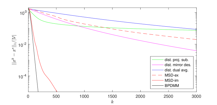
Figure 2: Convergence behavior of various distributed optimization algorithms.

Figure 2 shows that (MSD-ex) shares similar convergence behavior as the distributed mirror descent and the distributed dual averaging. This is mainly due the fact that both algorithms are based on explicit computation of subgradients, which requires diminishing step sizes to ensure convergence. On the other hand, (MSD-im) shares similar convergence behavior as BPDMM, as the implicit update allows a constant step size. The price is, in general, a more expensive computation at each iteration. Further, (MSD-im) almost achieves the same convergence speed as the BPDMM with a more efficient implementation, as pointed out in Remark 3.

5 Conclusions

In this paper, we have developed two novel algorithms for distributed optimization in non-Euclidean spaces based on the mass-spring-damper dynamics. Our results not only match those for centralized mirror descent, but also improve previous methods by allowing more efficient implementation. Nevertheless, the proposed algorithm has a few limitations, most notably, their mere applicability to undirected graphs. Our future research direction is motivated by this limitation, as well as extensions for smooth and stochastic optimization as well as time-varying graphs.

References

• [Açıkmeşe et al., 2014] Açıkmeşe, B., Mandić, M., and Speyer, J. L. (2014). Decentralized observers with consensus filters for distributed discrete-time linear systems. Automatica, 50(4):1037–1052.
• [Alvarez, 2000] Alvarez, F. (2000). On the minimizing property of a second order dissipative system in Hilbert spaces. SIAM J. Control Optim., 38(4):1102–1119.
• [Alvarez et al., 2002] Alvarez, F., Attouch, H., Bolte, J., and Redont, P. (2002). A second-order gradient-like dissipative dynamical system with Hessian-driven damping. Application to optimization and mechanics. J. Math. Pures Appl., 81(8):747–780.
• [Aubin and Cellina, 2012] Aubin, J.-P. and Cellina, A. (2012). Differential inclusions: set-valued maps and viability theory, volume 264. Springer Science & Business Media.
• [Beck and Teboulle, 2003] Beck, A. and Teboulle, M. (2003). Mirror descent and nonlinear projected subgradient methods for convex optimization. Oper. Res. Lett., 31(3):167–175.
• [Bertsekas and Tsitsiklis, 1989] Bertsekas, D. P. and Tsitsiklis, J. N. (1989). Parallel and Distributed Computation: Numerical Methods, volume 23. Prentice Hall Englewood Cliffs, NJ.
• [Boyd et al., 2011] Boyd, S., Parikh, N., Chu, E., Peleato, B., Eckstein, J., et al. (2011). Distributed optimization and statistical learning via the alternating direction method of multipliers. Found. Trends Mach. Learn., 3(1):1–122.
• [Bubeck et al., 2015] Bubeck, S. et al. (2015). Convex optimization: Algorithms and complexity. Found. Trends Mach. Learn., 8(3-4):231–357.
• [Censor and Lent, 1981] Censor, Y. and Lent, A. (1981). An iterative row-action method for interval convex programming. J. Optim. Theory Appl., 34(3):321–353.
• [Censor and Zenios, 1992] Censor, Y. and Zenios, S. A. (1992). Proximal minimization algorithm with D-functions. J. Optim. Theory Appl., 73(3):451–464.
• [Dekel et al., 2012] Dekel, O., Gilad-Bachrach, R., Shamir, O., and Xiao, L. (2012). Optimal distributed online prediction using mini-batches. J. Mach. Learn. Res., 13(1):165–202.
• [Doan et al., 2019] Doan, T. T., Bose, S., Nguyen, D. H., and Beck, C. L. (2019). Convergence of the iterates in mirror descent methods. IEEE Control Syst. Lett., 3(1):114–119.
• [Duchi et al., 2012] Duchi, J. C., Agarwal, A., and Wainwright, M. J. (2012). Dual averaging for distributed optimization: Convergence analysis and network scaling. IEEE Trans. Autom. Control, 57(3):592–606.
• [Gharesifard and Cortés, 2014] Gharesifard, B. and Cortés, J. (2014). Distributed continuous-time convex optimization on weight-balanced digraphs. IEEE Trans. Autom. Control, 59(3):781–786.
• [Gholami et al., 2016] Gholami, B., Yoon, S., and Pavlovic, V. (2016). Decentralized approximate bayesian inference for distributed sensor network. In Proc. AAAI Conf. Artificial Intell., pages 1582–1588.
• [Hatanaka et al., 2018] Hatanaka, T., Chopra, N., Ishizaki, T., and Li, N. (2018). Passivity-based distributed optimization with communication delays using PI consensus algorithm. IEEE Trans. Autom. Control, 63(12):4421–4428.
• [He and Yuan, 2012] He, B. and Yuan, X. (2012). On the O(1/n) convergence rate of the Douglas-Rachford alternating direction method. SIAM J. Numer. Anal., 50(2):700–709.
• [Kia et al., 2015] Kia, S. S., Cortés, J., and Martínez, S. (2015). Distributed convex optimization via continuous-time coordination algorithms with discrete-time communication. Automatica, 55:254–264.
• [Krichene et al., 2015] Krichene, W., Bayen, A., and Bartlett, P. L. (2015). Accelerated mirror descent in continuous and discrete time. In Proc. Int. Conf. Neural Inform. Process. Syst., pages 2845–2853.
• [Lesser et al., 2012] Lesser, V., Ortiz Jr, C. L., and Tambe, M. (2012). Distributed Sensor Networks: A Multiagent Perspective, volume 9. Springer Science & Business Media.
• [Levine et al., 2016] Levine, S., Finn, C., Darrell, T., and Abbeel, P. (2016). End-to-end training of deep visuomotor policies. J. Mach. Learn. Res., 17(1):1334–1373.
• [Li et al., 2002] Li, D., Wong, K. D., Hu, Y. H., and Sayeed, A. M. (2002). Detection, classification, and tracking of targets. IEEE Signal Process. Mag., 19(2):17–29.
• [Li et al., 2016] Li, J., Chen, G., Dong, Z., and Wu, Z. (2016). Distributed mirror descent method for multi-agent optimization with delay. Neurocomputing, 177:643–650.
• [Meng et al., 2015] Meng, D., Fazel, M., and Mesbahi, M. (2015). Proximal alternating direction method of multipliers for distributed optimization on weighted graphs. In Proc. IEEE Conf. Decision Control, pages 1396–1401. IEEE.
• [Mesbahi and Egerstedt, 2010] Mesbahi, M. and Egerstedt, M. (2010). Graph Theoretic Methods in Multiagent Networks. Princeton University Press.
• [Nedic and Ozdaglar, 2009] Nedic, A. and Ozdaglar, A. (2009). Distributed subgradient methods for multi-agent optimization. IEEE Trans. Autom. Control, 54(1):48–61.
• [Nedic et al., 2010] Nedic, A., Ozdaglar, A., and Parrilo, P. A. (2010). Constrained consensus and optimization in multi-agent networks. IEEE Trans. Autom. Control, 55(4):922–938.
• [Qiu et al., 2016] Qiu, Z., Liu, S., and Xie, L. (2016). Distributed constrained optimal consensus of multi-agent systems. Automatica, 68:209–215.
• [Raginsky and Bouvrie, 2012] Raginsky, M. and Bouvrie, J. (2012). Continuous-time stochastic mirror descent on a network: Variance reduction, consensus, convergence. In Proc. Conf. Decision Control, pages 6793–6800. IEEE.
• [Rockafellar, 1970] Rockafellar, R. T. (1970). Convex Analysis. Princeton University Press.
• [Wang and Banerjee, 2014] Wang, H. and Banerjee, A. (2014). Bregman alternating direction method of multipliers. In Proc. Int. Conf. Neural Inform. Process. Syst., pages 2816–2824.
• [Wang and Elia, 2010] Wang, J. and Elia, N. (2010). Control approach to distributed optimization. In Proc. Allerton Conf. Commun. Control Comput., pages 557–561. IEEE.
• [Wang and Elia, 2011] Wang, J. and Elia, N. (2011). A control perspective for centralized and distributed convex optimization. In Proc. IEEE Conf. Decision Control, pages 3800–3805. IEEE.
• [Wang et al., 2018] Wang, Y., Zhou, H., and Hong, Y. (2018). Distributed stochastic mirror descent algorithm over time-varying network. In Proc. Int. Conf. Control Automat., pages 716–721. IEEE.
• [Wei and Ozdaglar, 2012] Wei, E. and Ozdaglar, A. (2012). Distributed alternating direction method of multipliers. In Proc. IEEE Conf. Decision Control, pages 5445–5450. IEEE.
• [Wibisono et al., 2016] Wibisono, A., Wilson, A. C., and Jordan, M. I. (2016). A variational perspective on accelerated methods in optimization. Proc. Nat. Acad. of Sci., 113(47):E7351–E7358.
• [Xiao et al., 2007] Xiao, L., Boyd, S., and Kim, S.-J. (2007). Distributed average consensus with least-mean-square deviation. J. Parallel Distrib. Comput., 67(1):33–46.
• [Yahya et al., 2017] Yahya, A., Li, A., Kalakrishnan, M., Chebotar, Y., and Levine, S. (2017). Collective robot reinforcement learning with distributed asynchronous guided policy search. In Int. Conf. Intell. Robots Syst., pages 79–86. IEEE.
• [Yang et al., 2017] Yang, S., Liu, Q., and Wang, J. (2017). A multi-agent system with a proportional-integral protocol for distributed constrained optimization. IEEE Trans. Autom. Control, 62(7):3461–3467.
• [Yu et al., 2018] Yu, Y., Açıkmeşe, B., and Mesbahi, M. (2018). Bregman parallel direction method of multipliers for distributed optimization via mirror averaging. IEEE Control Syst. Lett., 2(2):302–306.
• [Yuan et al., 2018] Yuan, D., Hong, Y., Ho, D. W., and Jiang, G. (2018). Optimal distributed stochastic mirror descent for strongly convex optimization. Automatica, 90:196–203.
• [Zeng et al., 2017] Zeng, X., Yi, P., and Hong, Y. (2017). Distributed continuous-time algorithm for constrained convex optimizations via nonsmooth analysis approach. IEEE Trans. Autom. Control, 62(10):5227–5233.