Extinction Dynamics of Cardiac Fibrillation

Abstract

During episodes of atrial fibrillation, the heart’s electrical activity becomes disorganized and shows fragmenting spiral waves. To systematically address how this pattern terminates using spatially extended simulations exceeds current computational resources. To circumvent this limitation, we treat the number of spiral waves as a stochastic population with a corresponding birth-death equation and use techniques from statistical physics to determine the mean episode duration of atrial fibrillation. We show that this duration can be computed for arbitrary geometries in minimal computational time and that it depends exponentially on tissue size, consistent with the critical mass hypothesis which states that fibrillation requires a minimal organ size. Our approach can result in efficient and accurate predictions of mean episode duration, thus creating a potentially important step towards improved therapeutic interventions for atrial fibrillation.

I Introduction

Atrial fibrillation (AF) is the most common cardiac arrhythmia, affecting millions of people worldwide Chugh et al. (2013). During AF, the conduction pattern within atrial tissue becomes irregular, resulting in serious health consequences including heart failure, stroke, and mortality Fuster et al. (2006). Although the precise mechanisms for AF are still unclear, conduction patterns involving localized spiral waves (spiral waves with a tip location that remains within a certain spatial domain) have been shown to be a crucial component in the maintenance of this disease Jalife (2003); Nattel et al. (2017); Narayan et al. (2012a). The stable driving sources of AF can be eliminated using targeted ablation which destroys tissue. After the removal of driving sources, spiral wave reentry results in multiple and often migratory and transient waves of activation Narayan et al. (2012b); Haissaguerre et al. (2016); Narayan et al. (2012c). These spiral waves continuously break down to form new ones, and are removed through collisions with other spiral waves or with non-conducting boundaries as has been shown by many computational studies Karma (2013); Fenton et al. (2002); Zykov et al. (2017); Fink et al. (2011); Qu et al. (1999). This stochastic competition between creation and annihilation results in spiral defect chaos (SDC), a dynamical state described in a variety of different excitable systems Coullet et al. (1989); Egolf et al. (2000); Daniels and Bodenschatz (2002); Beta et al. (2006). SDC persists until the last spiral wave is terminated, with its duration representing a stochastic event.

Critical in AF management and therapy is thus the mean episode duration $\tau$ which is a statistical measure of the average time of reversal to normal sinus rhythm. The ability to infer $\tau$ from some observables of our system, particularly in the presence of different surgically created lesion sets and pharmacological interventions, can be an important step towards more efficient AF therapies and patient-specific ablation procedures Rotter et al. (2007); McDowell et al. (2012). Unfortunately, determining $\tau$ through direct simulations of spatially extended cardiac models is challenging because a statistically significant quantification of this stochastic quantity requires the time-consuming task of simulating a multitude of episodes Virag et al. (2002); Dossel et al. (2012). This becomes even more problematic for large geometry sizes since $\tau$ increases sharply as a function of the system size Qu (2006). This increase is related to the so-called critical mass hypothesis which posits that fibrillation requires atria with a minimal size Garrey (1914); Byrd et al. (2005). A fundamental elucidation for this hypothesis is currently lacking.

In this study, we develop an alternative method to compute $\tau$ by treating the number of spiral tips $n$ as a stochastic quantity and casting its birth-death process into a master equation, a commonly used approach in the field of population dynamics Lande et al. (2003); Van Kampen (1992); Gardiner (2009). This approach was also used in recent studies which examined filament turbulence in phenomenological models and which described the dynamics of surface defects in terms of a master equation Davidsen et al. (2008); Reid et al. (2011); St-Yves and Davidsen (2015). Contrary to these studies, we focus here on tips migrating in 2D and on termination events and the associated mean episode duration. In our case, the master equation describes the probability $P(n,t)$ of having $n$ spiral tips at time $t$ as

$$\frac{dP(n,t)}{dt}=\sum_{r}\left[W_{r}(n-r)P(n-r,t)-W_{r}(n)P(n,t)\right]$$ (1)

where $W_{r}$ are transition rates for the number of spiral tips to change by $r$ tips and can be computed directly from spatially extended simulations of cardiac models. Since tips are created and annihilated either as pairs or as singlets, we only need to consider $r=\pm 1,\pm 2$. As a boundary condition we take $n=0$ to be absorbing. This means that there is no escape from the no-tip state and that all birth rates for $n=0$ vanish: $W_{r}(0)=0$. Furthermore, an additional boundary condition stems from the fact that for $n=1$ the pair-wise death rate equals 0: $W_{-2}(1)=0$. Once the rates are known, we can construct a transition matrix which can be used to compute $\tau$ at minimal computational cost Newman (2010).

For large $n$, the death rate will exceed the birth rate since tips will have a high probability of colliding. As a result, the number of spiral tips does not grow to very large numbers. If for small $n$ the birth rate is larger than the death rate, then a long-lived (quasi-stationary) metastable state exists with a mean number of tips $\bar{n}$. The distribution associated with this metastable state is called the quasi-stationary distribution $P_{qs}(n)$ Dykman et al. (1994); Assaf and Meerson (2010). Note that for systems with an absorbing state at $n=0$, the stationary distribution trivially corresponds to $P(n)=0$ for all $n\neq 0$ and $P(0)=1$ In the quasi-stationary state, the number of tips fluctuates around the average value for prolonged periods of time and the mean episode duration can be computed using

$$\frac{1}{\tau}=\sum_{r<0}W_{r}(-r)P_{qs}(-r).$$ (2)

Termination only occurs during rare escape events, corresponding to a large fluctuation away from the mean number of tips. As a consequence, standard equilibrium statistical physics approaches based on small fluctuations do not apply Assaf and Meerson (2010); Doering et al. (2005). Instead, techniques from non-equilibrium statistical physics must be invoked to determine statistical quantities corresponding to extinction, including $\tau$.

To illustrate our stochastic approach to quantifying termination dynamics, we carry out simulations of SDC using spatially extended electrophysiological models. We should stress, however, that the approach should also work for other systems that exhibit spiral wave dynamics, including the complex Ginzburg-Landau equation Aranson and Kramer (2002) or simple phenomenological models Barkley et al. (1990). The “direct” simulations use the standard reaction-diffusion equation:

$${\partial_{t}V}=D\nabla^{2}V-I_{ion}/{C_{m}}$$ (3)

where $V$ is the transmembrane potential, $C_{m}$ ($\mu\rm{F}\,cm^{-2}$) is the membrane capacitance and $D\nabla^{2}$ expresses the inter-cellular coupling via gap junctions and diffusion constant $D$. The membrane currents in the electrophysiological model are denoted by $I_{ion}$ which are governed by nonlinear evolution equations coupled to $V$. For our purposes, the precise form of $I_{ion}$ is not important and we present results using the detailed Luo-Rudy (LR) model Luo and Rudy (1991), modified to obtain spiral wave break-up as described in Qu et al. Qu et al. (2000). To stress the generality of our approach we have also carried simulations using the simplified Fenton-Karma (FK) model (parameter set 8) Fenton and Karma (1998). Results from these simulations are shown in the Supplemental Material sup . We perform the simulations in square two-dimensional computational domains although our approach can be equally well applied in more complex geometries. As boundary conditions, we consider both non-conducting and periodic boundary conditions, and we vary the area of the computational domain, which is equivalent to varying $D$ while keeping the area constant. For both models, we use $C_{m}=1\mu$F/cm² while the diffusion constant is chosen to be $D=$0.0005 cm²/ms for the FK model and $D=$0.001 cm²/ms for the LR model. Simulations are carried out with a discretization of 0.025 cm, using a 5-point stencil, and a time step of 0.025 ms, using explicit Euler integration. For both models, the conduction velocity along a cable is within the electophysiological range: 51 cm/s for the FK model and 33 cm/s for the LR model. Errors in direct simulation results are reported as standard deviations.

II Results using direct simulations

Figure 1: Direct numerical simulations provide statistics of spiral tip dynamics. A: Snapshot of a simulation of the LR model in a 7.5$\times$7.5 cm computational domain with periodic boundary conditions. The voltage is represented using a color code with red (blue) corresponding to depolarized (repolarized) tissue. The location of the tips of counter- and clockwise rotation spiral waves are shown in black and white, respectively. (scale bar: 1cm) B: Typical time trace of the number of spiral tip pairs. For this particular simulation, spiral tips spontaneously extinguished after 8.3 s. C: Distribution of termination times for the direct simulations (symbols, computed using 400 termination events) and the master equation (solid line, computed using 10000 termination events).

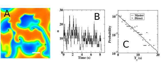
Starting with a random initial condition that contains multiple spiral waves, we solve the reaction-diffusion equation and keep track of the number of spiral tips using a standard algorithm (Fig. 1A) Fenton and Karma (1998). The number of tips fluctuates and the simulation ends after time $T_{e}$ when the number of spiral tips reaches 0 (Fig. 1B). We can compute the distribution of these termination times by repeating the simulations many times, starting with different and independent initial conditions. These conditions are created by perturbing a multi-spiral state with randomly placed stimuli in the form of a current stimulus of duration 20 ms and strength several times the excitation threshold. After perturbation, the system is allowed to evolve for another 100 ms before measurements are started. Our simulations reveal that this distribution is exponentially distributed, indicating that spiral wave termination can be well described as a Poisson process (Fig. 1C).

Next, we compute the birth and death rates as a function of the number of tips $n$ using different domain sizes with non-conducting boundaries by quantifying the number of transitions per time interval (Fig. 2A-D). For fixed computational time and domain size, the number of transitions will depend on the number of tips. It will become smaller as $n$ increases and no transitions will be recorded above some critical value of $n$. Here, to increase accuracy, we only consider rates that are computed using at least 100 transitions in the simulation. As a consequence, rates are computed up to a certain maximum value of $n$. In addition, for increasing domain sizes, transitions for small $n$ become increasingly rare. As a result, in large domains, the number of recorded transitions for small values of $n$ may not reach 100. The rates corresponding to these values of $n$ are therefore not included.

Examining the computed rates, we see that $W_{-1}$ depends linearly on the number of spiral tips for all domain sizes (Fig. 2A). The remaining rates, however, show a more complex dependence on the number of tips, indicating the existence of non-trivial long-range interactions between spiral tips (Fig. 2B-D). As a result, the rate curves are not easily fit by simple rational functions. Therefore, we employ a smoothing spline fit to the data to determine rates corresponding to transition events with less than the minimum number.

We can also compute the $W_{\pm 2}$ rates for domains that contain periodic boundary conditions. The results of these simulations are shown in the Supplemental Material sup and are qualitatively similar to the results presented in Fig. 2. As a consistency check, we can use these rates to compute the distribution of termination times. As expected, this distribution is exponential and agrees well with the one computed using direct simulations (Fig. 1C). In addition, we compute the rates for the FK model and show the results in the Supplemental Material sup .

Figure 2: Transition rates computed using direct simulations. A-D:The birth and death rates for $n\rightarrow n-1$ (A), $n\rightarrow n-2$ (B), $n\rightarrow n+1$ (C), $n\rightarrow n+2$ (D) computed in a square geometry of various sizes with non-conducting boundaries. Error bars represent standard deviation. E: The $W_{\pm 1}$ rates, normalized by the perimeter of the domain, as a function of the density of tips, $q=n/A$. F: The $W_{\pm 2}$ rates, normalized by the area of the domain, as a function of the density of tips.

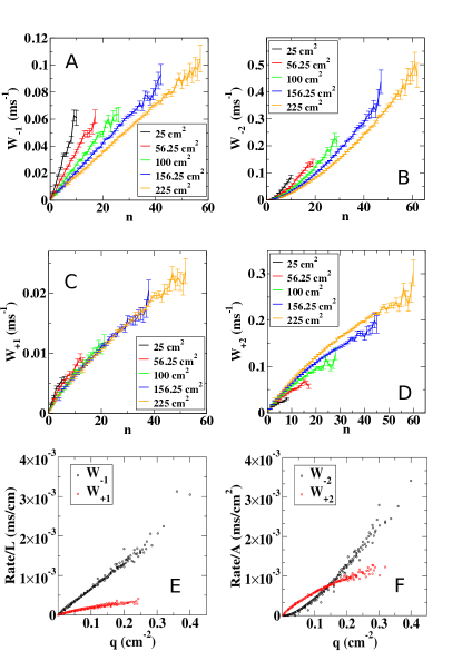
Importantly, we find that at large $A$ all rates collapse onto a single curve when plotted as a function of the density $q=n/A$. Specifically, the $W_{\pm 2}$ rates are found to scale with the area as $W_{\pm 2}(n)\sim Aw_{\pm 2}(q)$ (Fig. 2F), indicating that the birth and death rates only depend on the density and that tips are well-mixed. Furthermore, the $W_{\pm 1}$ rates scale with the perimeter $L$ as $W_{\pm 1}(n)\sim Lw_{\pm 1}(q)$ (Fig. 2E). Here, and in the following, we will take the continuum limit such that $q$ and functions that depend on this variable are considered to be continuous. Note that this observed linear scaling of $W_{-1}$ with $L$ implies that the death rate is proportional with the length of the non-conducting boundary and that creating ablation lesions will increase this rate. Furthermore, such scaling is expected if single tips annihilate through simple collision processes and get created near the boundaries. Similar scaling behavior is found for periodic boundary conditions and for the FK model, as shown in the Supplemental Material sup .

Figure 3: Dependence of spiral tip dynamics on the domain size. A, B: The quasi-stationary distribution for periodic (A) and non-conducting boundary conditions (B) using different domain sizes as computed using the transition matrix. The symbols show the quasi-stationary distribution as computed using the direct simulations. C: The average number of tips as a function of the area of the computational domain, computed using direct simulations (symbols) and using the master equation approach (line). The dashed curves are straight lines.

III Results using transition rates

Once the transition rates are determined, it is straightforward to compute the quasi-stationary distribution $P_{qs}(n)$ using the transition matrix at minimal computational cost (Fig. 3A, B) Newman (2010). For small domains, this can be carried out using the rates obtained in the simulations while for larger domains, where the rates for small $n$ cannot be computed accurately, we can use the interpolated rates. As the domain size increases, the distribution shifts to larger values of $n$, and becomes more symmetric around its peak. The average number of tips, $\bar{n}$, increases with system size and our simulations reveal that it depends linearly on the area of the computational domain for both boundary conditions (Fig. 3C). Results for the FK model and for periodic boundary conditions are qualitatively similar (see the Supplemental Material sup ).

For geometries that do not contain any non-conducting boundaries it is possible to derive closed-form solutions for the quasi-stationary distribution. In this case, $n$ is always even and tips will be created and annihilated in pairs such that $W_{\pm 1}=0$. The quasi-stationary distribution can be obtained by setting the left hand side in Eq. 1 to zero, resulting in the recursion relationship

$$P_{qs}(n)=P_{qs}(0)\prod_{j=2}^{n}W_{+2}(2j-2)/W_{-2}(2j)$$ (4)

where $P_{qs}(0)$ can be determined by the normalization condition $\sum_{n=0}^{\infty}P_{qs}(n)=1$ Gardiner (2009). The average number of tips can be obtained using

$$\frac{d<n>}{dt}=\frac{d}{dt}\left(\sum_{n^{\prime}=1}^{\infty}n^{\prime}P(n^{\prime})\right)$$ (5)

which results in a deterministic equation Gardiner (2009)

$$\frac{dn}{dt}=2W_{+2}(n)-2W_{-2}(n)$$ (6)

and a deterministic stationary state determined by $W_{+2}(n^{*})=W_{-2}(n^{*})$. The maximum value of the quasi-stationary distribution occurs for $P_{qs}(n-2)/P_{qs}(n)\approx 1$, corresponding to $W_{+2}(\bar{n}-2)=W_{-2}(\bar{n})$. Therefore, for large values of $A$ the stochastic average number can be well approximated by deterministic average number, $n^{*}\approx\bar{n}$. Furthermore, using our numerically found scaling, we obtain $w_{+2}(q^{*})=w_{-2}(q^{*})$, where $q^{*}=n^{*}/A$. Hence, the average density is independent of the area and $n^{*}$, and $\bar{n}$ scales with $A$, consistent with the scaling found in the simulations (Fig. 3C). For domains that contain non-conducting boundaries, the $\pm$1 rates are no longer zero and the corresponding deterministic equation reads

$$\frac{dn}{dt}=2W_{+2}(n)+W_{+1}(n)-2W_{-2}(n)-W_{-1}(n).$$ (7)

Using our obtained scaling, we have

$$2w_{+2}(q^{*})+w_{+1}(q^{*})/\sqrt{A}-2w_{-2}(q^{*})-w_{-1}(q^{*})/\sqrt{A}=0$$ (8)

and for large areas, the average number of tips will again scale linearly with the area.

IV Mean episode duration

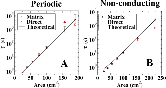
To find the mean episode duration $\tau$ in the direct simulations, we average the termination times $T_{e}$ obtained from each independent simulation. This computation becomes more and more time consuming as $A$ increases since termination becomes less and less likely. As a consequence, the number of determined termination events we consider vary from 400 for small domains to less than 10 for the largest areas still amenable to direct simulations. Our results reveal that $\tau$ displays an exponential dependence on the size of the domain, both for periodic (red symbols, Fig. 4A) and non-conducting boundary conditions (red symbols, Fig. 4B), consistent with earlier studies Qu (2006).

Figure 4: Termination times as a function of the system size. A, B: $\tau$ as a function of the area of the computational domain from direct simulations using domains with periodic boundary conditions (A) and non-conducting boundaries (B) (red symbols). Also shown are the results from the master equation approach (black symbols) and from the closed-form expression obtained using the WKB analysis (solid line). The red square represents the result of a single termination event computed using direct simulations while the solid red circle represents the computed time for a single computation that did not result in a termination.

Rather than using direct simulations to determine an average value for $T_{e}$, it is straightforward to use the interpolated transitions rates and the resulting transition matrix to compute $\tau$ using simple matrix operations Newman (2010). For this, we construct a transition matrix $Q$ for all transient states $n>0$, with elements $Q_{ij}$ representing the probability of transitioning from state $i$ to state $j$. The probability of reaching state $j$ from state $i$ in $t$ steps is then given by the $ij^{th}$ entry of $Q^{t}$. Summing this over all time results in the so-called fundamental matrix $N=I+Q+Q^{2}+...=(I-Q)^{-1}$, where $I$ is the identity matrix. Each element of the fundamental matrix $N_{ij}$ represents the mean duration our system will spend in state $j$ given an initial state $i$, which can be used to determine the quasi-stationary distribution. Moreover the mean time to extinction $\tau$ is given by $N\vec{e}$, where $\vec{e}$ is a column vector of ones. The confidence intervals for $\tau$ are computed through bootstrapping as follows. First we resample each transition rate by drawing a value from a binomial distribution with probability equal to the original transition rate and using the number of recorded transitions from the direct simulation. We then proceed by interpolating these resampled transition rates and computing $\tau$ from these interpolated transition rates. This is computed for 1000 trials and the confidence interval is determined from the 5th to the 95th percentile of the resulting $\tau$ across all trials web .

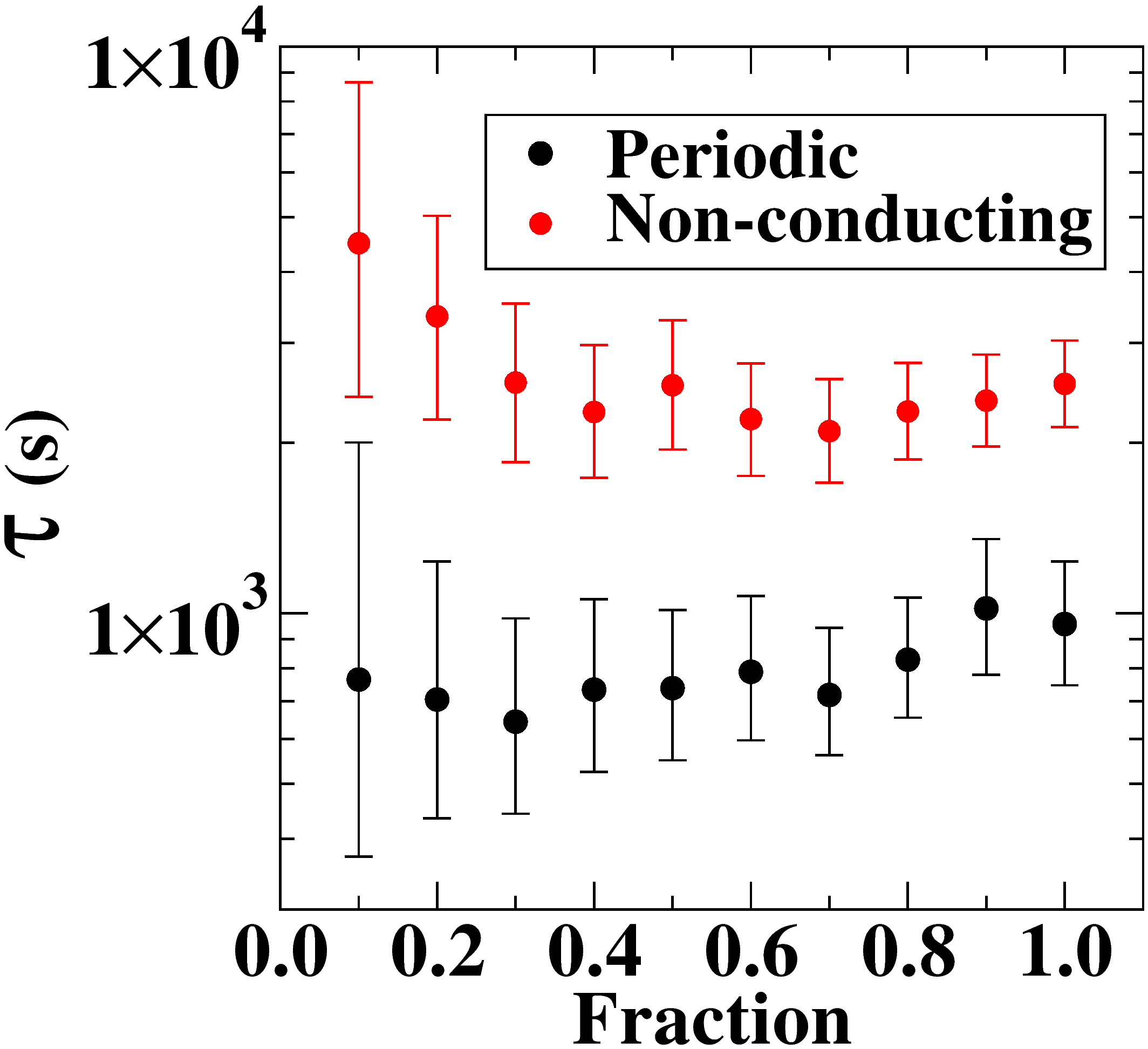
The resulting values for $\tau$ agree well with the direct numerical simulations (black symbols, Fig. 4A and B). Importantly, using the transition matrix allows us to estimate the mean episode duration for system sizes where determination of mean episode duration with direct simulations is impossible. For example, directly simulating a single extinction event on a domain with area $A=225\mu m^{2}$ and non-conducting boundaries was found to take approximately 100 hours of CPU time. Estimating $\tau$ from this single event is not useful as the error is large and generating a sufficient amount of termination events is not practical. Furthermore, for other larger domain sizes our direct simulations failed to produce a single termination event, even after 7 days of CPU time. Using the interpolated transition rates computed from this single, non-terminating event, however, we are still able to use the transition matrix (Fig. 4A and B) to predict the mean episode duration. Moreover, $\tau$ can already be estimated using only a fraction of the data, and thus simulation time, further demonstrating the power of the approach. This is shown in Fig. 5 where we plot $\tau$ as a function of the fraction of computational data from a direct simulation. Obviously, for larger fractions, the errors in the transition rates become smaller, resulting in smaller confidence intervals. Furthermore, the mean termination time converges as the fraction increases and can be reasonably well estimated from a small fraction of the entire dataset.

Figure 5: Accuracy of the master equation approach. The mean episode duration computed using the master equation as a function of the fraction of computational data obtained using direct simulations. Data segments of size indicated by fraction were started at random positions. Shown are the results for $A=225cm^{2}$ for the non-conducting case and for $A=189.0625cm^{2}$ for the periodic case. The error bars are determined using bootstrapping and represent the 5% and 95% confidence interval.

V Scaling results

We can also use our stochastic analysis of termination to determine the scaling of $\tau$ with the area. For periodic boundary conditions, it is possible to obtain an analytical expression for $\tau$   Gardiner (2009):

$$\tau(n_{0})=\sum_{k=1}^{n_{0}/2}\phi(2(k-1))\sum_{j=k}^{\infty}\frac{1}{\phi(2j){W}_{+2}(2j)}$$ (9)

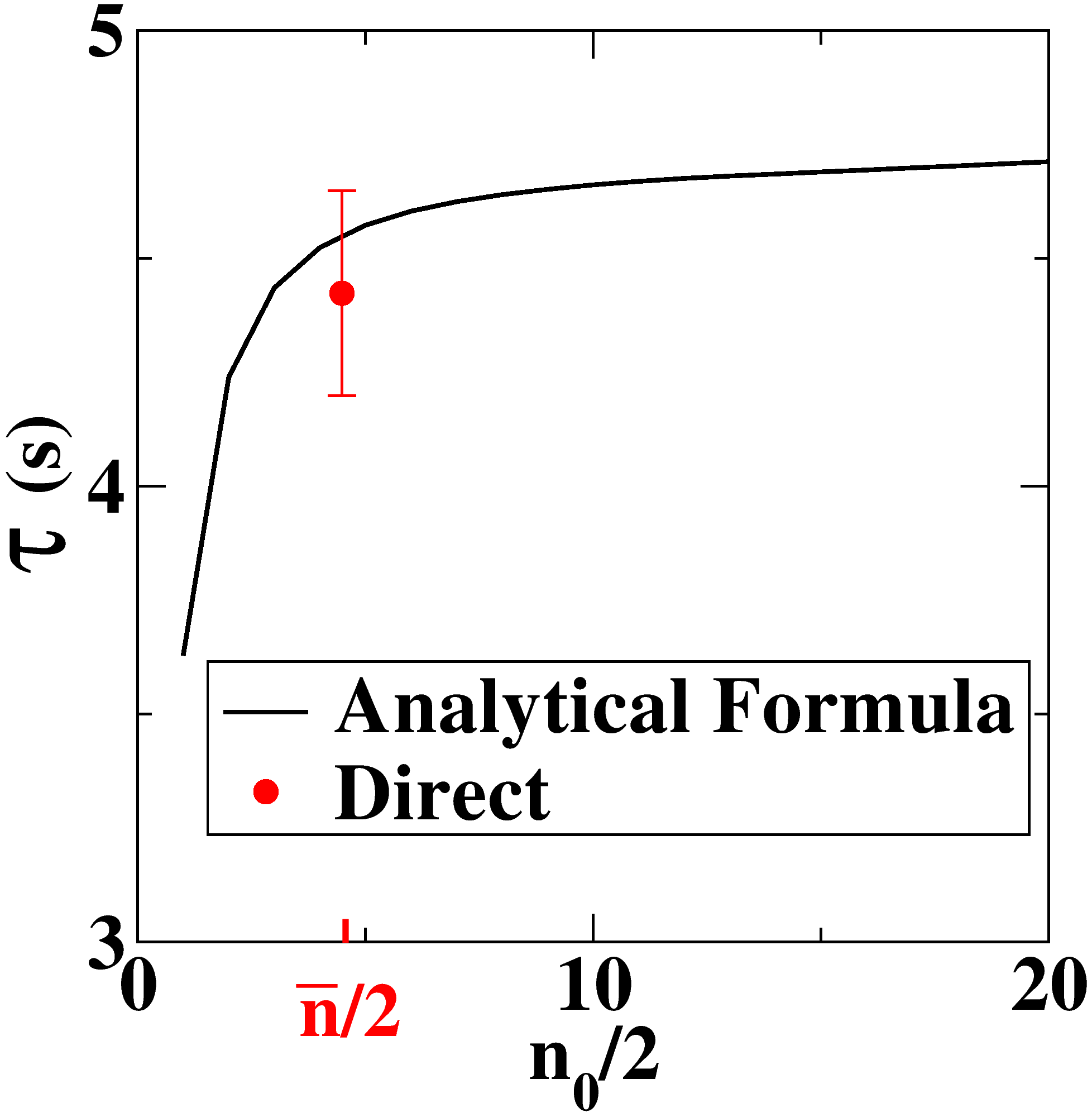
where $n_{0}$ is the initial number of spiral tips, $\phi(k)=\prod_{i=1}^{k/2}{W}_{-2}(2i)/{W}_{+2}(2i)$, and $\phi(0)\equiv 1$. Using the numerically determined rates we find that $\tau$ quickly converges as $n_{0}$ becomes large and that $\tau(\bar{n})$ agrees well with the values obtained using the numerical methods. This is shown explicitly in Fig. 6 which plots the mean episode duration as a function of the initial number of tips.

Figure 6: Analytical formula for periodic boundary conditions. Mean episode duration $\tau$ as computed using the analytical formula in the main text as a function of the initial number of tips, $n_{0}$. Symbol corresponds to the result from direct simulations ($\bar{n}\approx 9$). Shown are the results for the LR, using a domain of size 7.5cmx7.5cm.

To determine the scaling with the area we focus on the first term of this expression, $\tau(2)=\sum_{j=1}^{\infty}(\phi(2j){W}_{+2}(2j))^{-1}$. We can write $\phi(2j)$ as

$${\rm ln}\left[\phi(2j)\right]=\sum_{z=1}^{j}{\rm ln}\left[\frac{W_{-2}(2z)}{W_{+2}(2z)}\right]\approx-\frac{A}{2}\int_{2/A}^{x}{\rm ln}\frac{w_{+2}(s)}{w_{-2}(s)}\ ds$$ (10)

where we have used the fact that the transition rates scale with the area $A$ and have defined $s=2z/A$ and $x=2j/A$. As a result, the mean episode duration becomes

$$\tau\approx\int_{0}^{\infty}\frac{{\rm exp}\left[A\int_{2/A}^{x}{\rm ln}\sqrt{\frac{w_{+2}(s)}{w_{-2}(s)}}ds\right]}{2w_{+2}(x)}dx.$$ (11)

For large $A$, this integral will be sharply peaked around $q^{*}$. Thus, $\tau$ has the following scaling behavior Krapivsky et al. (2010):

$$\tau\sim{\rm exp}\left[A\int_{2/A}^{q^{*}}{\rm ln}\sqrt{\frac{w_{+2}(s)}{w_{-2}(s)}}ds\right]$$ (12)

and, as an immediate consequence of the observed scaling of the transition rates, we find that $\tau$ scales exponentially with the area, consistent with our direct numerical results (Fig. 4A).

We can also use approximation methods to determine the scaling of the mean episode duration by viewing the number of spiral tips as a stochastic population in a metastable state. This approach is particularly useful for domains containing non-conducting boundaries, for which it is no longer possible to derive an exact expression for $\tau$. As long as $A$, equivalent to the total population size in models of population biology, is sufficiently large, we can use a WKB approximation. In this approximation, the quasi-stationary distribution is assumed to obey $P_{qs}(q)\sim e^{-AS(q)}$ where $S(q)$ is a function called the action. We can now use our obtained scaling $W_{r}(n)=A^{r/2}w_{r}(q)$, together with the assumed form of $P_{qs}(q)$, and substitute them into the stationary form of Eq. 1. This equation is written in terms of the continuous rescaled variable $q=n/A$ so that $n-r\rightarrow q-r/A$ Assaf and Meerson (2010). For the periodic case, we take $S(q)=S_{0}(q)+O(A^{-1})$ while for absorbing boundaries, since the scaling of the $\pm 1$ rates goes as $\sqrt{A}$ while the $\pm 2$ rates go as $A$, we use $S(q)=S_{0}(q)+A^{-1/2}S_{1}(q)+O(A^{-1})$. The resulting equation can then be expanded in terms of $1/A$ which yields, to $O(1)$, a Hamilton-Jacobi equation

$$H(q,p)=\sum_{r}A^{r/2}w_{r}(q)(e^{rp}-1)=0$$ (13)

where $p(q)=\partial S/\partial q$ is the fluctuation momentum Dykman et al. (1994); Assaf and Meerson (2010).

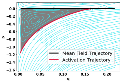
From the Hamiltonian $H$ we can define the dynamics of $p$ and $q$ using $\frac{dp}{dt}=-\frac{\partial{H}}{\partial q}$ and $\frac{dq}{dt}=\frac{\partial{H}}{\partial p}$. The non-trivial solution of $H(q,p_{a}(q))=0$ corresponds to the activation trajectory in the $q,p$ phase space Assaf and Meerson (2010); Kubo et al. (1973); Dykman et al. (1994); Kessler and Shnerb (2007); Doering et al. (2005). This trajectory describes the most probable path along which the system evolves from the metastable state $(q^{*},0)$ to a point $q$ in phase space. Since we are interested in extinction, we will consider the trajectory that connects $(q*,0)$ with $[0,p(0)]$, the so-called “optimal” path to extinction Dykman et al. (1994). This $q,p$ phase space, along with the activation trajectory, is shown in Fig. 7 for periodic boundaries and in the Supplemental Material for the FK model sup . The optimal path can be determined numerically but can also be determined using approximate closed-form relations. Specifically, for periodic boundary conditions, we find

$$S_{0}=\int_{q^{*}}^{2/A}\ln{\gamma_{0}}\ dq,$$ (14)

and $\gamma_{0}=\sqrt{\frac{w_{-2}}{w_{+2}}}$. In Fig. 7, this corresponds to the area between the activation trajectory and the $q$ axis, represented by the shaded part. Thus, we find that the mean episode duration scales as $\tau\sim e^{AS_{0}}$, consistent with Eq. 12. For absorbing boundaries, we can solve for $S_{1}$ perturbatively, yielding

$$S_{1}=\int_{q^{*}}^{2/A}\frac{(\gamma_{0}w_{+1}-w_{-1})(\gamma_{0}-1)}{2\gamma_{0}(w_{+2}-w_{-2})}dq.$$ (15)

Figure 7: WKB approach to spiral tip dynamics. Phase portrait of the Hamiltonian dynamics in $q$, $p$ space for periodic boundary conditions, showing the activation trajectory of the WKB Hamiltonian (red line). The shaded area represents the exponential factor $S_{0}$.

Using our formulation, we can now compute the mean episode duration for any system size once the rates for a single domain $\hat{A}$ are determined. Specifically, after computing for this particular domain both $\hat{S}_{0}$ and $\hat{S}_{1}$ and the corresponding mean episode duration $\hat{\tau}$, we can find $\tau$ as a function of the system size using:

$$\tau(A)\approx\hat{\tau}e^{(A-\hat{A})\hat{S}_{0}+(\sqrt{A}-\sqrt{\hat{A}})\hat{S}_{1}}.$$ (16)

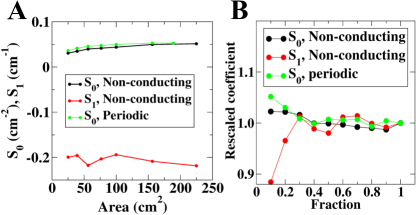
This scaling law for $\tau$ agrees well with the values of $\tau$ computed from the master equation, especially for larger values of $A$ (Fig. 4A, B), justifying the WKB approximation. For these larger domain sizes, the factors $S_{0}$ and $S_{1}$ converge, making the estimate from Eq. 16 to be more accurate, as shown in Fig. 8A. This is consistent with the obtained quasi-stationary distributions which become more symmetric around their peak value for larger domain size (Fig. 3A and B), rendering the WKB approximation more accurate. Furthermore, as is the case for $\tau$ (Fig. 5), both $S_{0}$ and $S_{1}$ can be estimated using the interpolated rates and only a fraction of the direct simulation data (Fig. 8B). Thus, accurate estimates for arbitrary domain sizes do not require simulating actual termination events. Finally, the exponential scaling of $\tau$ with system size $A$ reveals that, even though spiral wave driven fibrillation will always terminate, its mean episode duration depends critically on the size of the heart. Of course, this result is valid as long as the specifics of the model do not change. Other factors, including changes in electrophysiological parameters, can have an effect of mean termination duration. For large values of $A$, $\tau$ can be large while for very small values of $A$ as found, for example, in rodents, the mean episode duration will be well below 1 s. These findings provide a mechanistic underpinning for the well-established critical mass hypothesis which posits that fibrillation only occurs in hearts of a minimum size Garrey (1914); Qu (2006); Byrd et al. (2005).

Figure 8: WKB parameters as a function of area size for the LR model A: The exponential coefficients $S_{0}$ and $S_{1}$ as a function of domain size for periodic and non-conducting boundaries. B: The exponential factors $S_{0}$ and $S_{1}$, rescaled by their value computed at the largest computational data set, as a function of the fraction of computational data obtained using direct simulations. Data segments of size indicated by fraction were started at random positions. Shown are the results for $A=225cm^{2}$ for the non-conducting case and for $A=189.0625cm^{2}$ for the periodic case.

VI Summary

In summary, we present a novel approach to quantify spiral wave dynamics in spatially extended domains. This approach recasts the problem into a master equation, after which statistical physics methods can be employed. Our approach is valid for any model exhibiting SDC, including electrophysiological models, and any geometry. Key in this approach are the transition rates, which can be computed numerically from a limited set of direct simulations. Future work can include applying our approach to geometric models of atria. Geometry data are routinely obtained in patients and, combined with our analysis, might result in more patient-specific approaches for AF. In addition, it would be interesting to further study the dependence of the rates on the number of tips. If, for example, rational functions for these rates can be derived, it will be possible to obtain analytical expressions for $\tau$. Finally, it would be interesting to compare scaling of atrial fibrillation in healthy and diseased atria by simulating appropriate electrophysiological models. Thus, stochastic analysis of spiral wave reentry has the potential to be an important step towards determining optimal therapeutic interventions aimed at minimizing the duration of AF episodes.

VII Acknowledgements

We thank Brian A. Camley and David A. Kessler for valuable suggestions. We gratefully acknowledge support from the National Institutes of Health (R01 HL122384) and the American Heart Association (16PRE30930015).

References

- Chugh et al. (2013) S. S. Chugh, R. Havmoeller, K. Narayanan, D. Singh, M. Rienstra, E. J. Benjamin, R. F. Gillum, Y.-H. Kim, J. H. McAnulty, Z.-J. Zheng, et al., Circulation , CIRCULATIONAHA (2013).
- Fuster et al. (2006) V. Fuster, L. E. Rydén, D. S. Cannom, H. J. Crijns, A. B. Curtis, K. A. Ellenbogen, J. L. Halperin, J.-Y. Le Heuzey, G. N. Kay, J. E. Lowe, et al., Europace 8, 651 (2006).
- Jalife (2003) J. Jalife, Journal of cardiovascular electrophysiology 14, 776 (2003).
- Nattel et al. (2017) S. Nattel, F. Xiong, and M. Aguilar, Nature Reviews Cardiology (2017).
- Narayan et al. (2012a) S. M. Narayan, D. E. Krummen, and W.-J. Rappel, Journal of cardiovascular electrophysiology 23, 447 (2012a).
- Narayan et al. (2012b) S. M. Narayan, D. E. Krummen, K. Shivkumar, P. Clopton, W.-J. Rappel, and J. M. Miller, Journal of the American College of Cardiology 60, 628 (2012b).
- Haissaguerre et al. (2016) M. Haissaguerre, A. J. Shah, H. Cochet, M. Hocini, R. Dubois, I. Efimov, E. Vigmond, O. Bernus, and N. Trayanova, The Journal of physiology 594, 2387 (2016).
- Narayan et al. (2012c) S. M. Narayan, D. E. Krummen, M. W. Enyeart, and W.-J. Rappel, PLoS ONE 7, e46034 (2012c).
- Karma (2013) A. Karma, Annu. Rev. Condens. Matter Phys. 4, 313 (2013).
- Fenton et al. (2002) F. H. Fenton, E. M. Cherry, H. M. Hastings, and S. J. Evans, Chaos 12, 852 (2002).
- Zykov et al. (2017) V. Zykov, A. Krekhov, and E. Bodenschatz, Proceedings of the National Academy of Sciences 114, 1281 (2017).
- Fink et al. (2011) M. Fink, S. A. Niederer, E. M. Cherry, F. H. Fenton, J. T. Koivumäki, G. Seemann, R. Thul, H. Zhang, F. B. Sachse, D. Beard, et al., Progress in biophysics and molecular biology 104, 2 (2011).
- Qu et al. (1999) Z. Qu, J. N. Weiss, and A. Garfinkel, American Journal of Physiology-Heart and Circulatory Physiology 276, H269 (1999).
- Coullet et al. (1989) P. Coullet, L. Gil, and J. Lega, Physical review letters 62, 1619 (1989).
- Egolf et al. (2000) D. A. Egolf, I. V. Melnikov, W. Pesch, and R. E. Ecke, Nature 404, 733 (2000).
- Daniels and Bodenschatz (2002) K. E. Daniels and E. Bodenschatz, Physical review letters 88, 034501 (2002).
- Beta et al. (2006) C. Beta, A. S. Mikhailov, H. H. Rotermund, and G. Ertl, EPL (Europhysics Letters) 75, 868 (2006).
- Rotter et al. (2007) M. Rotter, L. Dang, V. Jacquemet, N. Virag, L. Kappenberger, and M. Haissaguerre, Pacing and clinical electrophysiology 30, 314 (2007).
- McDowell et al. (2012) K. S. McDowell, F. Vadakkumpadan, R. Blake, J. Blauer, G. Plank, R. S. MacLeod, and N. A. Trayanova, Journal of electrocardiology 45, 640 (2012).
- Virag et al. (2002) N. Virag, V. Jacquemet, C. Henriquez, S. Zozor, O. Blanc, J.-M. Vesin, E. Pruvot, and L. Kappenberger, Chaos: An Interdisciplinary Journal of Nonlinear Science 12, 754 (2002).
- Dossel et al. (2012) O. Dossel, M. W. Krueger, F. M. Weber, M. Wilhelms, and G. Seemann, Med Biol Eng Comput 50, 773 (2012).
- Qu (2006) Z. Qu, American Journal of Physiology-Heart and Circulatory Physiology 290, H255 (2006).
- Garrey (1914) W. E. Garrey, American Journal of Physiology–Legacy Content 33, 397 (1914).
- Byrd et al. (2005) G. D. Byrd, S. M. Prasad, C. M. Ripplinger, T. R. Cassilly, R. B. Schuessler, J. P. Boineau, and R. J. Damiano, Circulation 112, I (2005).
- Lande et al. (2003) R. Lande, S. Engen, and B.-E. Saether, Stochastic population dynamics in ecology and conservation (Oxford University Press on Demand, 2003).
- Van Kampen (1992) N. G. Van Kampen, Stochastic processes in physics and chemistry, Vol. 1 (Elsevier, 1992).
- Gardiner (2009) C. Gardiner, Stochastic Methods: A Handbook for the Natural and Social Sciences (Springer-Verlag, Berlin Heidelberg, 2009).
- Davidsen et al. (2008) J. Davidsen, M. Zhan, and R. Kapral, Physical review letters 101, 208302 (2008).
- Reid et al. (2011) J. Reid, H. Chaté, and J. Davidsen, EPL (Europhysics Letters) 94, 68003 (2011).
- St-Yves and Davidsen (2015) G. St-Yves and J. Davidsen, Physical Review E 91, 032926 (2015).
- Newman (2010) M. Newman, Networks; an introduction (Oxford University, Oxford, 2010).
- Dykman et al. (1994) M. Dykman, E. Mori, J. Ross, and P. Hunt, The Journal of chemical physics 100, 5735 (1994).
- Assaf and Meerson (2010) M. Assaf and B. Meerson, Physical Review E 81, 021116 (2010).
- Doering et al. (2005) C. R. Doering, K. V. Sargsyan, and L. M. Sander, Multiscale Modeling & Simulation 3, 283 (2005).
- Aranson and Kramer (2002) I. S. Aranson and L. Kramer, Reviews of Modern Physics 74, 99 (2002).
- Barkley et al. (1990) D. Barkley, M. Kness, and L. S. Tuckerman, Physical Review A 42, 2489 (1990).
- Luo and Rudy (1991) C. H. Luo and Y. Rudy, Circ Res 68, 1501 (1991).
- Qu et al. (2000) Z. Qu, F. Xie, A. Garfinkel, and J. N. Weiss, Ann Biomed Eng 28, 755 (2000).
- Fenton and Karma (1998) F. Fenton and A. Karma, Chaos 8, 20 (1998).
- (40) See Supplemental Material at http://link.aps.org/supplemental/xxx for additional figures.
- (41) Freely available code can be found at http://cardiacmap.ucsd.edu/.
- Krapivsky et al. (2010) P. L. Krapivsky, S. Redner, and E. Ben-Naim, A kinetic view of statistical physics (Cambridge University Press, 2010).
- Kubo et al. (1973) R. Kubo, K. Matsuo, and K. Kitahara, Journal of Statistical Physics 9, 51 (1973).
- Kessler and Shnerb (2007) D. A. Kessler and N. M. Shnerb, Journal of Statistical Physics 127, 861 (2007).