Probabilistic embeddings of the Fréchet distance

Abstract

The Fréchet distance is a popular distance measure for curves which naturally lends itself to fundamental computational tasks, such as clustering, nearest-neighbor searching, and spherical range searching in the corresponding metric space. However, its inherent complexity poses considerable computational challenges in practice. To address this problem we study distortion of the probabilistic embedding that results from projecting the curves to a randomly chosen line. Such an embedding could be used in combination with, e.g. locality-sensitive hashing. We show that in the worst case and under reasonable assumptions, the discrete Fréchet distance between two polygonal curves of complexity $t$ in ${\rm I\!R}^{d}$, where $d\in\{2,3,4,5\}$, degrades by a factor linear in $t$ with constant probability. We show upper and lower bounds on the distortion. We also evaluate our findings empirically on a benchmark data set. The preliminary experimental results stand in stark contrast with our lower bounds. They indicate that highly distorted projections happen very rarely in practice, and only for strongly conditioned input curves.

1 Introduction

The Fréchet distance is a distance measure for curves which naturally lends itself to fundamental computational tasks, such as clustering, nearest-neighbor searching, and spherical range searching in the corresponding metric space. However, their inherent complexity poses considerable computational challenges in practice. Indeed, spherical range searching under the Fréchet distance was recently the topic of the yearly ACM SIGSPATIAL GISCUP competition, highlighting the relevance and the difficulty of designing efficient data structures for this problem. At the same time, Afshani and Driemel showed lower bounds on the space-query-tradeoff in the pointer model [2] that demonstrate that this problem is even harder than simplex-range searching.

The computational complexity of computing a single Fréchet distance between two given curves is a well-studied topic [3, 10, 11, 12, 13, 18, 21]. It is believed that it takes time that is quadratic in the length of the curves and this running time can be achieved by applying dynamic programming. In this body of literature, the case of 1-dimensional curves under the continuous Fréchet distance stands out. In particular, no lower bounds are known on computing the continuous Fréchet distance between 1-dimensional curves. It has been observed that the problem has a special structure in this case [14]. Clustering under the Fréchet distance can be done efficiently for 1-dimensional curves [19], but seems to be harder for curves in the plane or higher dimensions. Bringmann and Künnemann used projections to lines to speed up their approximation algorithm for the Fréchet distance [12]. They showed that the distance computation can be done in linear time if the convex hulls of the two curves are disjoint. It is tempting to believe that the curves being restricted to 1-dimensional space makes the problem significantly easier. However, in the general case, there are no algorithms known which are faster for 1-dimensional curves than for curves in higher dimensions. In practice, it is very common to separate the coordinates of trajectories to simplify computational tasks. It seems that in practice the inherent character of a trajectory is often largely preserved when restricted to one of the coordinates of the ambient space. Mathematically, this amounts to projecting the trajectory to a line.

This motivates our study of probabilistic embeddings of the Fréchet distance into the space of 1-dimensional curves. Concretely, we study distortion of the probabilistic embedding that results from projecting the curves to a randomly chosen line. Such a random projection could be used in combination with probabilistic data structures, e.g. locality-sensitive hashing [20], but also with the multi-level data structures for Fréchet range searching given by Afshani and Driemel [2]. See below for a more in-depth discussion of these data structures.

We show that in the worst case and under certain assumptions, the discrete Fréchet distance between two polygonal curves of complexity $t$ in ${\rm I\!R}^{d}$, where $d=\{2,3,4,5\}$, degrades by a factor linear in $t$ with constant probability. In particular, we show upper and lower bounds on the change in distance for the class of $c$-packed curves. The notion of the $c$-packed curves was introduced by Driemel, Har-Peled and Wenk in [18] and has proved useful as a realistic input assumption [4, 10, 17]. A curve is called $c$-packed for a value $c>0$ if the length of the intersection of the curve with any ball of any radius $r$ is a most $cr$. While our study is mostly restricted to the discrete Fréchet distance, we expect that our techniques can be extended to the case of the continuous Fréchet distance.

A closely related distance measure, which is popular in the field of data-mining, is dynamic time warping (DTW) [16, 32, 34]. The computational complexity of DTW has also been extensively studied, both empirically and in theory [1, 4, 24, 30]. Some of our lower bounds extend to DTW.

1.1 Related work on data structures with Fréchet distance

The complexity of classic data structuring problems for the Fréchet distance is still not very well-understood, despite several papers on the topic. We review what is known for nearest-neighbor searching and range searching. Indyk [28] gave a deterministic and approximate near-neighbor data structure for the discrete Fréchet distance. A $c$-approximate nearest-neighbor data structure returns for a given query point $q$ a data point $p\in S$, such that the distance $d(p,q)$ is at most $c\cdot d(p^{*},q)$, where $p^{*}\in S$ is the true nearest neighbor to $q$. Indyk’s data structure for data set $S$, containing $n$ curves which have at most $t$ vertices, achieves approximation factor $c\in{\mathcal{O}\!\left({\log t+\log\log n}\right)}$ and has query time ${\mathcal{O}\!\left({\operatorname{poly}(t)\log n}\right)}$. This data structure requires large space, as it precomputes all queries with curves with $\sqrt{t}$ vertices. For short curves (with $t\in{\mathcal{O}\!\left({\log n}\right)}$) Driemel and Silvestri [20] described an approximate near-neighbor structure based on locality-sensitive hashing with approximation factor ${\mathcal{O}\!\left({t}\right)}$, query time ${\mathcal{O}\!\left({t\log n}\right)}$, using space ${\mathcal{O}\!\left({n\log n+tn}\right)}$. LSH is a technique that uses families of hash functions with the property that near points are more likely to be hashed to the same index than far points. Driemel and Silvestri were the first to define locality-sensitive hash functions for the discrete Fréchet distance. Emiris and Psarros [22] improved their result and also showed how to obtain $(1+\varepsilon)$-approximation with query time $\tilde{\mathcal{O}}\left(d\cdot 2^{2t}\cdot\log n\right)$ and using space $\tilde{\mathcal{O}}(n)\cdot\left(2+d/\log t\right)^{{\mathcal{O}\!\left({t\cdot d\cdot\log(1/\varepsilon)}\right)}}$. No such hash functions are known for the continuous case. It is conceivable that the concept of signatures which was introduced by Driemel, Krivošija and Sohler [19] in the context of clustering of 1-dimensional curves could be used to define an LSH for the continuous case and that this technique could be used in combination with projections to random lines.

De Berg et al. [15] studied range counting data structures for spherical range search queries under the continuous Fréchet distance assuming that the centers of query ranges are line segments. This data structure stores compressed subcurves using a partition tree, using space ${\mathcal{O}\!\left({s\operatorname{polylog}(n)}\right)}$ and query time ${\mathcal{O}\!\left({(n/\sqrt{s})\operatorname{polylog}(n)}\right)}$ to obtain a constant approximation factor, where $n\leq s\leq n^{2}$ is a parameter to the data structure which is fixed at preprocessing time.

Afshani and Driemel recently showed how to leverage semi-algebraic range searching for this problem [2]. Their data structure also supports polygonal curves of low complexity and answers queries exactly. In particular, for the discrete Fréchet distance they described a data structure which uses space in ${\mathcal{O}\!\left({n(\log\log n)^{t_{s}-1}}\right)}$ and achieves query time in ${\mathcal{O}\!\left({n^{1-1/d}\cdot\log^{{\mathcal{O}\!\left({t_{s}}\right)}}n\cdot t_{q}^{{\mathcal{O}\!\left({d}\right)}}}\right)}$, where $t_{s}$ denotes the complexity of an input curve and it is assumed that the complexity of the query curves $t_{q}$ is upper-bounded by a polynomial of $\log n$. For the continuous Fréchet distance they described a data structure for polygonal curves in the plane which uses space in ${\mathcal{O}\!\left({n(\log\log n)^{{\mathcal{O}\!\left({t_{s}^{2}}\right)}}}\right)}$ and achieves query time in ${\mathcal{O}\!\left({\sqrt{n}\log^{{\mathcal{O}\!\left({t_{s}^{2}}\right)}}n}\right)}$. For the case where the curves lie in dimension higher than $2$ and the distance measure is the continuous Fréchet distance, no data structures for range searching or range counting are known.

1.2 Related work on metric embeddings

Given metric spaces $(X,d_{X})$ and $(Y,d_{Y})$, we call a metric embedding an injective mapping $f:X\rightarrow Y$. We call $c$, $c\geq 1$, the distortion of the embedding $f$ [29] if there is an $r\in(0,\infty)$ such that for all $x,y\in X$ it is $r\cdot d_{X}(x,y)\leq d_{Y}(f(x),f(y))\leq c\cdot r\cdot d_{X}(x,y)$.

The work that is perhaps closest to ours is a recent result by Backurs and Sidiropoulos [6]. They gave an embedding of the Hausdorff distance into constant-dimensional $\ell_{\infty}$ space with constant distortion. More precisely, for any $s,d\geq 1$, they obtained an embedding for the Hausdorff distance over point sets of size $s$ in $d$-dimensional space, into $\ell_{\infty}^{s^{{\mathcal{O}\!\left({s+d}\right)}}}$ with distortion $s^{{\mathcal{O}\!\left({s+d}\right)}}$. No such metric embeddings are known for the discrete or continuous Fréchet distance. It has been shown that the doubling dimension of the Fréchet distance is unbounded, even in the case when the metric spaces is restricted to curves of constant complexity [19]. A result of Bartal et al. [9] for doubling spaces implies that a metric embedding of the Fréchet distance into an $\ell_{p}$ space would have at least super-constant distortion, but it is not known how to find such an embedding.

We discuss what is known on two variations of the metric embedding problem that are most studied. The first is to find the smallest distortion for any metric from the given class. Matoušek [31] showed that any metric on a point set of size $s$ can be embedded into $d$-dimensional Euclidean space with multiplicative distortion ${\mathcal{O}\!\left({\min\{s^{2/d}\log^{3/2}s,s\}}\right)}$, but not better than $\Omega\left(s^{1/\lfloor(d+1)/2\rfloor}\right)$. For $d=1$ this implies that the distortion is linear in the worst case.

The second problem is to find the smallest approximation factor to a minimal distortion for a given metric over a point set of size $s$. We call a spread $\Delta$ a maximum/minimum ratio of the distances of the input point set $X$. Badoiu et al. [7] gave an ${\mathcal{O}\!\left({\Delta^{3/4}c^{11/4}}\right)}$-approximation to the embedding to a line, where $c$ is the distortion of embedding of the input set onto the line. They also showed that it is hard to approximate this problem up to a factor $\Omega\left(n^{1/12}\right)$, even for a weighted tree metrics with polynomial spread. Assuming a constant distortion $c$ and a polynomial spread $\Delta$, Nayyeri and Raichel [33] gave a ${\mathcal{O}\!\left({1}\right)}$-approximation algorithm to the minimal distortion of the embedding to a line, in time polygonal in $s$ and $\Delta$. See the work of Badoiu et al. [8], Fellows et al. [23], Håstad et al. [25], and Indyk [27] for further reading.

1.3 Our results

Given two polygonal curves $P$ and $Q$ with $t$ vertices each from $\mathbb{R}^{d}$, where $d\in\{2,3,4,5\}$. Consider sampling a unit vector u in respective $\mathbb{R}^{d}$ uniformly at random, and let $P^{\prime}$ and $Q^{\prime}$ be the projections of the two curves to the line supporting u. We observe that Fréchet distance always decreases when the curves are projected to a line (Lemma 2.4). We show that if the curves $P$ and $Q$ are $c$-packed for constant $c$, then, with constant probability, the discrete Fréchet distance between the curves $P$ and $Q$, denoted by $d_{F}\!\left({P,Q}\right)$, degrades by at most a linear factor in $t$. This is stated by Theorem 1.1 for $d\in\{2,3\}$, and by Theorem 1.2 for $d\in\{4,5\}$.

Theorem 1.1.

Given $c\geq 2$, for any two polygonal $c$-packed curves $P$ and $Q$ from $\mathbb{R}^{2}$ or $\mathbb{R}^{3}$, and for any $\gamma\in(0,1)$ it holds that

$$\emph{Pr}\left[\frac{d_{F}\!\left({P,Q}\right)}{d_{F}\!\left({P^{\prime},Q^{\prime}}\right)}\leq\frac{12c+16}{\gamma}\cdot t\right]\geq 1-\gamma.$$

Theorem 1.2.

Given $c\geq 2$, for any two polygonal $c$-packed curves $P$ and $Q$ from $\mathbb{R}^{4}$ or $\mathbb{R}^{5}$, and for any $\gamma\in(0,1)$ it holds that

$$\emph{Pr}\left[\frac{d_{F}\!\left({P,Q}\right)}{d_{F}\!\left({P^{\prime},Q^{\prime}}\right)}\leq\left(1+\frac{2}{\pi}\right)\cdot\frac{12c+16}{\gamma}\cdot t\right]\geq 1-\gamma.$$

We also present a lower bound on the ratio of the two distances. The construction of the lower bound uses $c$-packed curves with $c<3$.

Theorem 1.3.

Given $c\geq 2$, there exist polygonal $c$-packed curves $P$ and $Q$, such that for any $\gamma\in(0,1/\pi)$

$$\emph{Pr}\left[\frac{d_{F}\!\left({P,Q}\right)}{d_{F}\!\left({P^{\prime},Q^{\prime}}\right)}\geq\frac{5\pi\gamma}{6}\cdot t\right]\geq 1-\gamma.$$

Theorem 1.3 holds for the continuous Fréchet distance and for dynamic time warping distance as well.

We also show that there exist polygonal curves $P$ and $Q$ that are not $c$-packed for sublinear $c$ and their (continuous or discrete) Fréchet distance degrades by a linear factor for any projection line (i.e. with probability 1). Theorem 4.1 presents this result.

2 Preliminaries

Throughout the paper we use the following notational conventions. Consider two polygonal curves $P=\{p_{1},p_{2},\ldots,p_{t}\}$ and $Q=\{q_{1},q_{2},\ldots,q_{t}\}$ in $\mathbb{R}^{d}$ given by their sequences of vertices. We choose a unit vector u in $\mathbb{R}^{d}$ by choosing a point on the $(d-1)$-dimensional unit hypersphere uniformly at random. We denote with $L$ the line through the origin that supports the vector u. Let $P^{\prime}=\{p^{\prime}_{1},p^{\prime}_{2},\ldots,p^{\prime}_{t}\}$ and $Q^{\prime}=\{q^{\prime}_{1},q^{\prime}_{2},\ldots,q^{\prime}_{t}\}$ be the projections of $P$ and $Q$ to $L$, defined by $p^{\prime}_{i}=\left\langle p_{i},\textbf{u}\right\rangle$ and $q^{\prime}_{j}=\left\langle q_{j},\textbf{u}\right\rangle$, for all $1\leq i\leq t$ and $1\leq j\leq t$. We denote $\delta_{i,j}=\|p_{i}-q_{j}\|$ and $\delta^{\prime}_{i,j}=\|p^{\prime}_{i}-q^{\prime}_{j}\|$, for all $1\leq i\leq t$ and $1\leq j\leq t$, i.e. $\delta_{i,j}$ and $\delta^{\prime}_{i,j}$ are the pairwise distances of the vertices for the input curves $P$ and $Q$ and for their respective projections $P^{\prime}$ and $Q^{\prime}$.

We define the discrete Fréchet distance of $P$ and $Q$ as follows: we call a traversal $T$ of $P$ and $Q$ a sequence of pairs of indices $(i,j)$ of vertices $(p_{i},q_{j})\in P\times Q$ such that

1. the traversal $T$ starts with $(1,1)$ and ends with $(t,t)$, and

2. the pair $(i,j)$ of $T$ can be followed only by one of $(i+1,j)$, $(i,j+1)$ or $(i+1,j+1)$.

We notice that every traversal is monotone. If $\mathcal{T}$ is the set of all traversals $T$ of $P$ and $Q$, then the discrete Fréchet distance between $P$ and $Q$ is defined as

$$d_{F}\!\left({P,Q}\right)=\min_{T\in\mathcal{T}}\max_{(i,j)\in T}\|p_{i}-q_{j}\|.$$ (1)

Furthermore, we define a directed, vertex-weighted graph $G=(V,E)$ on the node set $V=\{(i,j):1\leq i,j\leq t\}$. A node $(i,j)$ corresponds to a pair of vertices $p_{i}$ of $P$ and $q_{j}$ of $Q$ and we assign it the weight $\delta_{i,j}$. The set of edges is defined as $E=\{\left((i,j),(i^{\prime},j^{\prime})\right):i^{\prime}\in\{i,i+1\},j^{\prime}=\{j,j+1\},1\leq i,i^{\prime},j,j^{\prime}\leq t\}$. The set of paths in the graph $G$ between $(1,1)$ and $(t,t)$ corresponds to the set of traversals $\mathcal{T}$. We call a path in $G$ which does not start in $(1,1)$ or end in $(t,t)$ a partial traversal of $P$ and $Q$.

It is useful to picture the nodes of the graph $G$ as a matrix, where rows correspond to the vertices of $P$ and columns correspond to the vertices of $Q$. For any fixed value $\Delta>0$, we define the free-space matrix $F_{\Delta}=\left(\phi_{i,j}\right)_{1\leq i,j\leq t}$ with

$$\phi_{i,j}=\begin{cases}1&\text{if }\|p_{i}-q_{j}\|<\Delta\\ 0&\text{if }\|p_{i}-q_{j}\|\geq\Delta.\end{cases}$$

Overlaying the graph with the free-space matrix for $\Delta>d_{F}\!\left({P,Q}\right)$, we can observe that there exists a path in the graph from $(1,1)$ to $(t,t)$ that visits only the matrix entries with value $1$. Moreover, the existence of such a path in the free-space matrix for some value of $\Delta$ implies that $\Delta>d_{F}\!\left({P,Q}\right)$.

We define $c$-packedness of curves as follows.

Definition 2.1 ($c$-packed curve).

Given $c>0$, a curve $P\in\mathbb{R}^{d}$ is $c$-packed if for any point $p\in\mathbb{R}^{d}$ and any radius $r>0$, the total length of the curve $P$ inside the hypersphere $\texttt{ball}\!\left({p,r}\right)$ is at most $c\cdot r$.

We prove the following basic fact about random projections to a line, stated for $d\in\{2,3\}$ by Lemma 2.2, and for $d\in\{4,5\}$ by Lemma 2.3. For a general problem in much higher dimension $d$, the probability stated by these lemmas cannot be bounded by a linear function in $\varphi$, due to the measure concentration around $\pi/2$.

Lemma 2.2.

If two points $p$ and $q$ are projected to the straight line $L$, which supports the unit vector chosen uniformly at random on the unit hypersphere in $\mathbb{R}^{2}$ or $\mathbb{R}^{3}$, the probability that the distance of their projections will be reduced from the original distance by a factor greater than $\varphi$ is at most $\varphi$.

Proof.

Figure 1: The projection of the pair of the vertices to the straight line

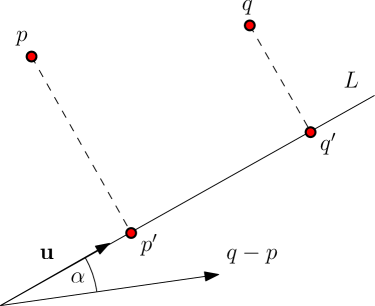
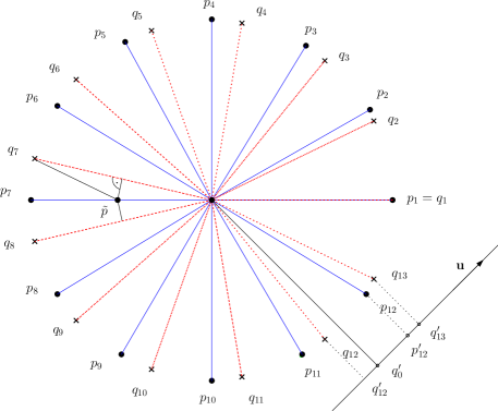
Let $p$ and $q$ be two vertices in $\mathbb{R}^{d}$. Let u be the unit vector chosen uniformly at random on the unit hypersphere and let $L$ be the straight line that supports the vector u. Then let $p^{\prime}$ and $q^{\prime}$ be the projections of $p$ and $q$ respectively to the projection line $L$, and let $\alpha$ be the angle between u and the vector $q-p$ (see Figure 1). Then it holds by the definion of the inner product that

$$\|q^{\prime}-p^{\prime}\|=\|\left\langle q-p,\textbf{u}\right\rangle\cdot\textbf{u}\|=\|q-p\|\cdot\|u\|\cdot|\cos\alpha|\cdot\|u\|.$$ (2)

It is $|\cos\alpha|\geq\varphi$ for $\alpha\in\left[0,\arccos\varphi\right]\cup\left[\pi-\arccos\varphi,\pi\right]$, for any $\varphi\in[0,1]$.

A $d$-sphere is a $d$-dimensional manifold that can be embedded in Euclidean $(d+1)$-dimensional space. A $d$-sphere with radius $R$ has the volume $V_{d}(R)$ and the surface area $S_{d}(R)$ given by:

$$V_{d}(R)=\frac{\pi^{\frac{d}{2}}}{\Gamma\left(\frac{d}{2}+1\right)}\cdot R^{d}\hskip 14.22636pt\text{ and }\hskip 14.22636ptS_{d}(R)=\frac{2\pi^{\frac{d+1}{2}}}{\Gamma\left(\frac{d+1}{2}\right)}\cdot R^{d}.$$

$\Gamma(z)$ is the gamma function defined as

$$\Gamma(z)=\int_{0}^{\infty}x^{z-1}e^{-x}dx$$

for all $z\in\mathbb{R}$, which is a known extension of the factorial function to the set of real numbers, satisfying $\Gamma(1/2)=\sqrt{\pi}$, $\Gamma(1)=1$ and $\Gamma(n+1)=n\cdot\Gamma(n)$ (for all $n\in\mathbb{N}$) [5, 26].

Since the projection line $L$ supports the vector u, which is chosen uniformly at random on the unit hypersphere in $\mathbb{R}^{d}$ ($(d-1)$-sphere with radius 1), the angle $\alpha$ is distributed by the probability distribution function $h_{d}(\alpha)$, defined as the ratio of the surface of a $(d-2)$-sphere of radius $\sin\alpha$ and the surface of a unit $(d-1)$-sphere. This can be expressed as:

$$h_{d}\left(\alpha\right)=\frac{1}{\sqrt{\pi}}\cdot\frac{\Gamma\left(\frac{d}{2}\right)}{\Gamma\left(\frac{d-1}{2}\right)}\cdot\left(\sin\alpha\right)^{d-2}$$ (3)

over the interval $\alpha\in\left[0,\pi\right]$.

For $d=2$ the distribution of $\alpha$ in Equation (3) is uniform with $h_{2}(\alpha)=1/\pi$. Thus

$$\text{Pr}\left[\frac{\|q^{\prime}-p^{\prime}\|}{\|q-p\|}\geq\varphi\right]=\text{Pr}\left[|\cos\alpha|\geq\varphi\right]=\frac{2\arccos\varphi}{\pi}$$ (4)

and

$$\text{Pr}\left[\frac{\|q^{\prime}-p^{\prime}\|}{\|q-p\|}<\varphi\right]=1-\frac{2\arccos\varphi}{\pi}.$$

Using Taylor series of $\arccos\varphi$ we get for $0\leq\varphi\leq 1$:

$$\arccos\varphi = \frac{\pi}{2}-\sum_{k=0}^{\infty}\frac{(2k)!\cdot\varphi^{2k+1}}{2^{2k}\cdot(2k+1)\cdot(k!)^{2}}=\frac{\pi}{2}-\varphi-\sum_{k=1}^{\infty}\frac{(2k)!\cdot\varphi^{2k+1}}{2^{2k}\cdot(2k+1)\cdot(k!)^{2}}$$

$$\geq \frac{\pi}{2}-\varphi-\varphi^{3}\cdot\sum_{k=1}^{\infty}\frac{(2k)!}{2^{2k}\cdot(2k+1)\cdot(k!)^{2}}=\frac{\pi}{2}-\varphi-\varphi^{3}\cdot\left(\frac{\pi}{2}-1\right)$$

since $\varphi\geq\varphi^{3}\geq\varphi^{2k+1}$ for all $k\geq 1$. Therefore

$$\text{Pr}\left[\frac{\|q^{\prime}-p^{\prime}\|}{\|q-p\|}<\varphi\right]=1-\frac{2\arccos\varphi}{\pi}\leq\frac{2}{\pi}\cdot\varphi+\left(1-\frac{2}{\pi}\right)\cdot\varphi^{3}\leq\varphi.$$ (5)

For $d=3$ the distribution of $\alpha$ in Equation (3) is $h_{3}(\alpha)=\left(\sin\alpha\right)/2$ for $\alpha\in[0,\pi]$. Thus

$$\text{Pr}\left[|\cos\alpha|\geq\varphi\right]=\text{Pr}\left[\alpha\in[0,\arccos\varphi]\cup[\pi-\arccos\varphi,\pi]\right]=2\cdot\int_{0}^{\arccos\varphi}\frac{\sin\alpha}{2}d\alpha=1-\varphi$$

due to the symmetry of $h_{3}(\alpha)$ around $\pi/2$. Therefore it holds that

$$\text{Pr}\left[\frac{\|q^{\prime}-p^{\prime}\|}{\|q-p\|}<\varphi\right]=1-\left(1-\varphi\right)=\varphi.$$ (6)

The claim of the lemma follows from Equations (5) and (6). ∎

Lemma 2.3.

If two points $p$ and $q$ are projected to the straight line $L$, which supports the unit vector chosen uniformly at random on the unit hypersphere in $\mathbb{R}^{4}$ or $\mathbb{R}^{5}$, the probability that the distance of their projections will be reduced from the original distance by a factor greater than $\varphi$ is at most $\left(1+2/\pi\right)\cdot\varphi$.

Proof.

We extend the proof of Lemma 2.2 to the cases $d=4$ and $d=5$ as follows.

For $d=4$ the distribution of $\alpha$ in Equation (3) is $h_{4}(\alpha)=\left(2\sin^{2}\alpha\right)/\pi$ for $\alpha\in[0,\pi]$. Thus

$$\text{Pr}\left[\frac{\|q^{\prime}-p^{\prime}\|}{\|q-p\|}<\varphi\right]=1-2\cdot\int_{0}^{\arccos\varphi}\frac{2}{\pi}\sin^{2}\alpha d\alpha=1-\frac{2}{\pi}\left[\arccos\varphi-\varphi\cdot\sqrt{1-\varphi^{2}}\right].$$

Using the last two inequalities of (5), this implies that

$$\text{Pr}\left[\frac{\|q^{\prime}-p^{\prime}\|}{\|q-p\|}<\varphi\right]\leq\varphi+\frac{2}{\pi}\cdot\varphi\cdot\sqrt{1-\varphi^{2}}\leq\left(1+\frac{2}{\pi}\right)\cdot\varphi.$$ (7)

For $d=5$ the distribution of $\alpha$ in Equation (3) is $h_{5}(\alpha)=\left(3\sin^{3}\alpha\right)/4$ for $\alpha\in[0,\pi]$. Due to the symmetry of $h_{5}(\alpha)$ around $\pi/2$ it holds that

$$\text{Pr}\left[\frac{\|q^{\prime}-p^{\prime}\|}{\|q-p\|}<\varphi\right]=1-2\cdot\int_{0}^{\arccos\varphi}\frac{3}{4}\sin^{3}\alpha d\alpha=\frac{9}{8}\cdot\varphi-\frac{1}{8}\cos\left(3\arccos\varphi\right)\leq\left(1+\frac{2}{\pi}\right)\cdot\varphi.$$ (8)

The last inequality of (8) follows from the fact that the function $f(\varphi)=(2/\pi-1/8)\cdot\varphi+\cos\left(3\arccos\varphi\right)/8$ is monotone and increasing, and it holds that $f(0)=0$.

The claim of the lemma follows from Equations (7) and (8). ∎

For the sake of completeness we prove the following lemma.

Lemma 2.4.

Given two curves $P=\{p_{1},\ldots,p_{t}\}$ and $Q=\{q_{1},\ldots,q_{t}\}$ in $\mathbb{R}^{d}$, and let $P^{\prime}=\{p^{\prime}_{1},\ldots,p^{\prime}_{t}\}$ and $Q^{\prime}=\{q^{\prime}_{1},\ldots,q^{\prime}_{t}\}$ respectively be their projections to the straight line $L$ which supports the vector u chosen uniformly at random on the unit hypersphere in $\mathbb{R}^{d}$. It holds that $d_{F}\!\left({P,Q}\right)\geq d_{F}\!\left({P^{\prime},Q^{\prime}}\right)$.

Proof.

Let $d_{F}\!\left({P,Q}\right)>d_{F}\!\left({P^{\prime},Q^{\prime}}\right)$ for some projection line $L$, and let $T$ and $T^{\prime}$ be the traversals of $P$ and $Q$, and $P^{\prime}$ and $Q^{\prime}$ that realize $d_{F}\!\left({P,Q}\right)$ and $d_{F}\!\left({P^{\prime},Q^{\prime}}\right)$ respectively. $T,T^{\prime}\in\mathcal{T}$, where $\mathcal{T}$ is the set of all traversals of $P$ and $Q$ (and also of $P^{\prime}$ and $Q^{\prime}$). Then it holds that

$$d_{F}\!\left({P,Q}\right)=\max_{(i,j)\in T}\|p_{i}-q_{j}\|<\max_{(i,j)\in T^{\prime}}\|p^{\prime}_{i}-q^{\prime}_{j}\|\leq\max_{(i,j)\in T^{\prime\prime},T^{\prime\prime}\in\mathcal{T}}\|p^{\prime}_{i}-q^{\prime}_{j}\|.$$

For any $(i,j)\in T^{\prime\prime}$, $T^{\prime\prime}\in\mathcal{T}$, we denote with $\alpha_{i,j}$ the angle between the vectors $q_{j}-p_{i}$ and $q^{\prime}_{j}-p^{\prime}_{i}$ (the latter being parallel to u). Since any traversal of $P^{\prime}$ and $Q^{\prime}$ is a traversal of $P$ and $Q$, using Equation (2) it holds that

$$d_{F}\!\left({P,Q}\right)<\max_{(i,j)\in T}\|p^{\prime}_{i}-q^{\prime}_{j}\|=\max_{(i,j)\in T}\|p_{i}-q_{j}\|\cdot|\cos\alpha_{i,j}|\leq\max_{(i,j)\in T}\|p_{i}-q_{j}\|,$$

a contradiction. ∎

3 Upper bound

3.1 Guarding sets

The discrete Fréchet distance between curves $P$ and $Q$ is realized by some pair $(p_{i},q_{j})$ of vertices $p_{i}\in P$ and $q_{j}\in Q$, being at the distance $\|p_{i}-q_{j}\|=\delta$. We would like to apply Lemma 2.2 to this pair of vertices to show that the distance is preserved up to some constant factor. However, it is possible that the pairwise distances in the projection are such that a cheaper traversal is possible that avoids the pair $(p_{i},q_{j})$ altogether. Therefore, we will apply the lemma to a subset of pairs of vertices of $P$ and $Q$ whose distance is large (e.g. larger than $\Delta=\delta/\theta$ for some small value of $\theta\geq 1$) and such that the chosen set forms a hitting set for the set of traversals $\mathcal{T}$. To this end we introduce the notion of the guarding set by the following definition.

Definition 3.1 (Guarding set).

For any two polygonal curves $P=\{p_{1},\ldots,p_{t}\}$ and $Q=\{q_{1},\ldots,q_{t}\}$ and a given parameter $\theta\geq 1$, a $\theta$-guarding set $B\subseteq V$ for $P$ and $Q$ is a subset of the set of vertices of $G$ that satisfies the following conditions:

1. (distance property) for all $(i,j)\in B$, it holds that $\delta_{i,j}\geq d_{F}\!\left({P,Q}\right)/\theta$, and

2. (guarding property) for any traversal $T$ of $P$ and $Q$, it is $T\cap B\neq\emptyset$.

Note that the set $B$ “guards” every traversal of $P$ and $Q$ in the sense that any path in $G$ from $(1,1)$ to $(t,t)$ has non-empty intersection with $B$. In other words, $B$ is a hitting set for the set of traversals $\mathcal{T}$.

For a guarding set $B$ we define the subset of vertices $S_{B}\subseteq V$ that can be reached by a path in $G$ starting from $(1,1)$ without visiting a vertex of $B$. We also define the subset of vertices $H_{B}=V\setminus(B\cup S_{B})$. A guarding set $B$ thus defines a vertex partition of the graph $G$ into three subsets $V=S_{B}\cup B\cup H_{B}$.

We show the following simple lemma for $d\in\{2,3\}$, and its counterpart for $d\in\{4,5\}$, given by Lemma 3.3.

Lemma 3.2.

Given parameter $\theta\geq 1$, if $B$ is a $\theta$-guarding set for the given curves $P=\{p_{1},\ldots,p_{t}\}$ and $Q=\{q_{1},\ldots,q_{t}\}$ from $\mathbb{R}^{2}$ or $\mathbb{R}^{3}$, and if $P^{\prime}$ and $Q^{\prime}$ are their projections to the straight line $L$, whose support unit vector u is chosen uniformly at random on the unit hypersphere, then for any $\beta>1$ it holds that

$$\frac{d_{F}\!\left({P^{\prime},Q^{\prime}}\right)}{d_{F}\!\left({P,Q}\right)}\geq\frac{1}{\beta\cdot\theta\cdot|B|}$$

with positive constant probability at least $1-1/\beta$.

Proof.

Let u be the unit vector which is chosen uniformly at random on the unit hypersphere in $\mathbb{R}^{d}$ with $d\in\{2,3\}$, and let u be supported by the projection line $L$. Let $\alpha_{i,j}$ be the angle between u and the vector $q_{j}-p_{i}$, for $i,j\in\{1,\ldots,t\}$. If we consider the distances of the pairs of the points $(p_{i},q_{j})\in P\times Q$, represented by the elements $(i,j)\in B$, then the probability of the event that some of these distances of the points of $P$ and $Q$ is reduced by a factor greater than $\beta\cdot|B|$ (the “bad” event) when projected to $L$ can be bounded by the union bound inequality and by Lemma 2.2 for $\varphi=\frac{1}{\beta|B|}$ as:

$$\text{Pr}\left[\left(\exists(i,j)\in B\right):\frac{\delta^{\prime}_{i,j}}{\delta_{i,j}}<\frac{1}{\beta|B|}\right]\leq\sum_{(i,j)\in B}\text{Pr}\left[\frac{\delta^{\prime}_{i,j}}{\delta_{i,j}}<\frac{1}{\beta|B|}\right]\leq\sum_{(i,j)\in B}\frac{1}{\beta|B|}=\frac{1}{\beta}$$ (9)

for any $\beta>1$.

Since by Definition 3.1 any traversal $T$ of $P$ and $Q$ has nonempty intersection with $B$, the Fréchet distance of $P$ and $Q$ has to be at least as big as the distance of some pair $(i,j)\in T\cap B$. These pairs of vertices have distance at least $d_{F}\!\left({P,Q}\right)/\theta$, and they are going to be reduced at most by the factor $\beta\cdot|B|$ (with positive constant probability). The traversal $T^{\prime}$ of $P^{\prime}$ and $Q^{\prime}$ that realizes $d_{F}\!\left({P^{\prime},Q^{\prime}}\right)$ has to contain at least one of the pairs of $B$ by Definition 3.1, since the pairs of the traversal $T^{\prime}$ are simultaneously the pairs of the traversal $T$ of $P$ and $Q$ (that contains the pairs of the vertices of $P$ and $Q$ in the same order as the pairs of their projections in $P^{\prime}$ and $Q^{\prime}$). Thus $d_{F}\!\left({P^{\prime},Q^{\prime}}\right)\geq d_{F}\!\left({P,Q}\right)/\left(\beta\cdot\theta\cdot|B|\right)$, which proves the lemma. ∎

Lemma 3.3.

Given parameter $\theta\geq 1$, if $B$ is a $\theta$-guarding set for the given curves $P=\{p_{1},\ldots,p_{t}\}$ and $Q=\{q_{1},\ldots,q_{t}\}$ from $\mathbb{R}^{4}$ or $\mathbb{R}^{5}$, and if $P^{\prime}$ and $Q^{\prime}$ are their projections to the straight line $L$, whose support unit vector u is chosen uniformly at random on the unit hypersphere, then for any $\beta>1$ it holds that

$$\frac{d_{F}\!\left({P^{\prime},Q^{\prime}}\right)}{d_{F}\!\left({P,Q}\right)}\geq\frac{1}{\left(1+2/\pi\right)\cdot\beta\cdot\theta\cdot|B|}$$

with positive constant probability at least $1-1/\beta$.

Proof.

We adapt the proof of Lemma 3.2 as follows: the probability of the “bad” event – that one of the distances of the points of $P$ and $Q$ is reduced by a factor greater than $\left(1+2/\pi\right)\cdot\beta\cdot|B|$, when projected to $L$, is bounded by the union bound inequality and Lemma 2.3 for $\varphi=1/\left(\left(1+2/\pi\right)\cdot\beta\cdot|B|\right)$ as:

$$\text{Pr}\left[\left(\exists(i,j)\in B\right):\frac{\delta^{\prime}_{i,j}}{\delta_{i,j}}<\frac{1}{\left(1+2/\pi\right)\cdot\beta\cdot|B|}\right] \leq \sum_{(i,j)\in B}\text{Pr}\left[\frac{\delta^{\prime}_{i,j}}{\delta_{i,j}}<\frac{1}{\left(1+2/\pi\right)\cdot\beta\cdot|B|}\right]$$

$$\leq \sum_{(i,j)\in B}\frac{1+2/\pi}{\left(1+2/\pi\right)\cdot\beta\cdot|B|}=\frac{1}{\beta},$$

for any $\beta>1$. The rest of the argumentation of the proof of Lemma 3.3 is analogous to the proof of Lemma 3.2. ∎

Intuitively we think of $\delta^{\prime}_{i,j}$ as an approximation to $\delta_{i,j}$. Lemma 3.2 yields a naive $\left(\beta\cdot t^{2}\right)$-approximation for any $\beta>1$ and $\theta=1$. Let $B$ be the set of all pairs $(i,j)\in\{1,\ldots,t\}\times\{1,\ldots,t\}$ such that $\|p_{i}-q_{j}\|=\delta_{i,j}\geq d_{F}\!\left({P,Q}\right)$. In the worst case $B$ could contain all $t^{2}$ pairs. Set $B$ is a $1$-guarding set. The correctness of the condition a) of Definition 3.1 is provided directly by the definition of $B$. The condition b) follows by contradiction. If there would exist some traversal $T$ such that $T\cap B=\emptyset$, then for all pairs $(i,j)\in T$ it would have to hold that $\|p_{i}-q_{j}\|<d_{F}\!\left({P,Q}\right)$. But then the traversal $T$ would witness that $d_{F}\!\left({P,Q}\right)\leq\max_{(i,j)\in T}\|p_{i}-q_{j}\|<d_{F}\!\left({P,Q}\right)$, a contradiction.

One could obtain better constant $\beta$ by more technical argument, which we omit here. Clearly, the approximation factor of Lemma 3.2 can be improved by the better choice of the set $B$. This question we explore in the following section.

3.2 Improved analysis for c-packed curves

In order to ensure that the number of the pairs of the indices that take part in the sum in the union bound inequality in (9) is not quadratic but at most a linear one in terms of the input size, we have to carefully select a small subset that satisfies the guarding set properties.

3.2.1 Building of the initial guarding set

We first give the simple construction of a $\theta$-guarding set for any $\theta\geq 1$ by Algorithm 1.

Data: $\delta=d_{F}\!\left({P,Q}\right)$, vertex-weighted graph $G=(V,E)$

Result: set $B$

1 $B\leftarrow\emptyset$;

2 if $\delta_{1,1}\geq\delta/\theta$ then

3       $B\leftarrow\{(1,1)\}$

4else

       FIFO-Queue $\mathcal{Q}\leftarrow\{(1,1)\}$;

        /* Breadth-First-Search on $G=(V,E)$ */

5       while $\mathcal{Q}\neq\emptyset$ do

6            

7            $(i,j)\leftarrow\text{pop}(\mathcal{Q})$;

8             foreach $((i,j),(i^{\prime}j^{\prime}))\in E$ do

9                   if $\delta_{i,j}<\delta/\theta$ and $\delta_{i^{\prime},j^{\prime}}<\delta/\theta$ then

10                        push$(\mathcal{Q},(i^{\prime},j^{\prime}))$;

11                        

12                  else if $\delta_{i,j}<\delta/\theta$ and $\delta_{i^{\prime},j^{\prime}}\geq\delta/\theta$ then

13                         $B\leftarrow B\cup\{(i^{\prime},j^{\prime})\}$;

14                        

15                  

16            

17      return $B$

Algorithm 1 Computing the $\theta$-guarding set, $\theta\geq 1$

Lemma 3.4.

The set $B$ obtained by Algorithm 1 is a $\theta$-guarding set, for any $\theta\geq 1$.

Proof.

We have to show that the resulting set $B$ satisfies the conditions of Definition 3.1. In the case that the distance $\delta_{1,1}\geq\delta/\theta$, it suffices to assign $B=\{(1,1)\}$, since any traversal of the curves $P$ and $Q$ has to include the pair $(1,1)$. For the rest of the proof let $\delta_{1,1}<\delta/\theta$.

Algorithm 1 selects into $B$ only the pairs $(i^{\prime},j^{\prime})$ with $\delta_{i^{\prime},j^{\prime}}\geq\delta/\theta$ in the line 12, and that are reached by an edge from a pair $(i,j)$ with $\delta_{i,j}\leq\delta/\theta$. Thus the condition a) of Definition 3.1 is satisfied by the yielded set. For the condition b) we show by induction the following invariant: in each point of time during the BFS, any traversal $T$ contains either a vertex of $B$ or a vertex in the queue $\mathcal{Q}$. The BFS starts with $(1,1)\in\mathcal{Q}$ with $\delta_{1,1}<\delta/\theta$. While processing the pair in $(i,j)\in\mathcal{Q}$ with $\delta_{i,j}<\delta/\theta$ during the BFS (lines 7 and 8) the traversal $T$ may use one of the pairs $(i+1,j)$, $(i,j+1)$ or $(i+1,j+1)$ (connected by the edges in $E$). The next pair in the traversal $T$ is either added into $\mathcal{Q}$ (line 10), or added into $B$ (line 12). In both cases the invariant remains valid. Since the queue is empty at the end, this means that any traversal contains a vertex in $B$, as claimed. ∎

  $F_{\delta/\theta}=\left(\begin{matrix}\includegraphics[width=138.76157pt]{forklike_marked}\end{matrix}\right)$

Figure 2: The curves $P$ and $Q$ (left) that yield a “fork-like” free-space matrix $F_{\delta/\theta}$ for some $\theta\geq 1$ (right). The pairs selected into $B$ by Algorithm 1 are marked with the red bound.

Unfortunately, the set $B$ built by Algorithm 1 can have a quadratic number of elements in terms of the input size, like the one in Figure 2 (marked with the red bound). If the free-space matrix $F_{\delta/\theta}$ would have the “fork-like” structure for some $\theta\geq 1$, such that for every column $j$ with $j\mod 3=1$ it holds for all pairs $\delta_{i,j}<\delta/\theta$ and thus $\phi_{i,j}=1$ (except for $\delta_{t,j}\geq\delta/\theta$), and for every column $j$ with $j\mod 3=2$ there are all pairs with $\delta_{i,j}\geq\delta/\theta$ and thus $\phi_{i,j}=0$ (except for $\delta_{1,j}<\delta/\theta$). For the columns with $j\mod 3=0$ let $\phi_{1,j}=1$, $\phi_{2,j}=0$ and $\phi_{t,j}=0$ (the rest may be filled arbitrarily). Then the set $B$ built by Algorithm 1 would contain $\left(t-1\right)\cdot t/3={\mathcal{O}\!\left({t^{2}}\right)}$ entries. We note that this cannot happen if the curves $P$ and $Q$ are $c$-packed for some constant $c$, $c\geq 2$, as it will be discussed in the further text.

3.2.2 On the structure of the distance matrix

Lemma 3.5 states one property of the $c$-packed curves, which we apply in Lemma 3.6.

Lemma 3.5.

Given point $p$ and a $c$-packed curve $Q=\{q_{1},\ldots,q_{t}\}$ from $\mathbb{R}^{d}$, then for any value $b>0$ there exists a value $r\in[b/2,b]$, such that the hypersphere centered at $p$ with radius $r$ intersects or is tangent to at most $2c$ edges of $Q$.

Proof.

Assume for the sake of contradiction that there exists $c^{\prime}>2c$, such that for any $r\in[b/2,b]$ there are at least $c^{\prime}$ edges of $Q$ that intersect or are tangent the surface of the hypersphere $\texttt{ball}\!\left({p,r}\right)$. Let the event points be the points in $\texttt{ball}\!\left({p,b}\right)\setminus\texttt{ball}\!\left({p,b/2}\right)$, such that they are either

1. vertices $q_{i}$ of $Q$ or

2. the points $q^{\prime}\in\overline{q_{i}q_{i+1}}$, such that $\overline{pq^{\prime}}\perp\overline{q_{i}q_{i+1}}$.

Let the set of events be $\mathcal{R}=\{R_{1},\ldots,R_{\ell}\}$, and let $r_{i}=\|p-R_{i}\|$ for all $1\leq i\leq\ell$. We may assume that the events $R_{i}$ are sorted ascending by $r_{i}$. Let $r_{0}=b/2$ and $r_{\ell+1}=b$, thus $r_{0}\leq r_{1}\leq\ldots\leq r_{\ell+1}$.

The number of the edges of $Q$ that intersect or are tangent to $\texttt{ball}\!\left({p,r}\right)$ is equal for all $r^{\prime}\in\left[r_{i},r_{i+1}\right)$ and for all $0\leq i\leq\ell$, since the number of such edges changes only in event points. After assumption there are at least $c^{\prime}$ edges of $Q$ that intersect $\texttt{ball}\!\left({p,r^{\prime}}\right)$, for any $r^{\prime}\in\left[r_{i},r_{i+1}\right)$ and for any $0\leq i\leq\ell$. The length of the curve $Q$ within $\texttt{ball}\!\left({p,b}\right)\setminus\texttt{ball}\!\left({p,b/2}\right)$ is

$$\sum_{i=0}^{\ell}\|Q\cap\left(\texttt{ball}\!\left({p,r_{i+1}}\right)\setminus\texttt{ball}\!\left({p,r_{i}}\right)\right)\|=\|Q\cap\left(\texttt{ball}\!\left({p,b}\right)\setminus\texttt{ball}\!\left({p,\frac{b}{2}}\right)\right)\|\leq c\cdot b$$

since $Q$ is $c$-packed. But on the other side it is

$$\sum_{i=0}^{\ell}\|Q\cap\left(\texttt{ball}\!\left({p,r_{i+1}}\right)\setminus\texttt{ball}\!\left({p,r_{i}}\right)\right)\|\geq\sum_{i=0}^{\ell}c^{\prime}\cdot|r_{i+1}-r_{i}|=c^{\prime}\cdot\left(b-\frac{b}{2}\right)>c\cdot b,$$

a contradiction. ∎

Lemma 3.6.

Given point $p$ and a $c$-packed curve $Q=\{q_{1},\ldots,q_{t}\}$ from $\mathbb{R}^{d}$, and given a value $b>0$, then for any pairwise disjoint set of intervals

$$I\subseteq\{[i_{1},i_{2}]~{}|~{}i_{1}\leq i_{2}\in{\rm I\!N},1\leq i_{1}\leq i_{2}\leq t\}$$

with $d(p,q_{i})\geq b$ for all $i\in[i_{1},i_{2}]\in I$, there exists a value of $r\in[b/2,b]$ and a pairwise disjoint set of intervals

$$J\subseteq\{[j_{1},j_{2}]~{}|~{}j_{1}\leq j_{2}\in{\rm I\!N},1\leq j_{1}\leq j_{2}\leq t\}$$

with the following properties:

1. $|J|\leq c+1$

2. $~{}\forall~{}[j_{1},j_{2}]\in J~{}\exists~{}i_{1}\leq i_{2}<i_{3}\leq i_{4}~{}:~{}[i_{1},i_{2}],[i_{3},i_{4}]\in I\wedge j_{1}=i_{1}\wedge j_{2}=i_{4}$

3. $~{}\forall~{}i\in[j_{1},j_{2}]\in J~{}:~{}d(p,q_{i})\geq r$

Proof.

We set $r$ to be the value of the same variable as in Lemma 3.5. Now we construct the set $J$ by merging intervals of $I$ as follows. Initially $J$ is empty. We iterate over the intervals of $I$ in the order of their starting points. Consider the first interval $[i_{1},i_{2}]$ and the next interval in the order $[i_{3},i_{4}]$, we merge them into one interval $[i_{1},i_{4}]$ if there exists no point $q_{j}$ with $i_{2}<j<i_{3}$ such that $d(p,q_{j})<r$. We continue merging this interval with the intervals in $I$ until we found a point $q_{j}$ such that $d(p,q_{j})<r$. Then, we add the current merged interval to $J$ and take the next interval from $I$ and merge it with the proceeding intervals in the same manner. When there are no intervals left in $I$, we also add the current interval to $J$. Each time we add an interval to $J$ (except possibly for the last one), we encountered two edges of $Q$ that intersect the sphere of radius $r$ centered at $p$. By Lemma 3.5 we have added at most $c+1$ intervals to $J$ (including the last interval). The other properties stated in the lemma follow by construction of $J$. Figure 3 illustrates the merging process. ∎

Figure 3: The process of Lemma 3.6 for the vertex $p$ and the curve $Q$

3.2.3 Avoidable pairs

Definition 3.7 (Avoidable pair).

Let $B$ be the $\theta$-guarding set produced by Algorithm 1, and let $V=S_{B}\cup B\cup H_{B}$ be the partition of $V$ implied by $B$. The pair $(i,j)\in B$ is called avoidable if there exist a pair $(i^{\prime},j^{\prime})\in B$ and two partial traversals $T_{1}$ and $T_{2}$ of $P$ and $Q$ from $(1,1)$ to $(i^{\prime},j^{\prime})$, such that:

1. $\forall(i^{\prime\prime},j^{\prime\prime})\in\left(T_{1}\cup T_{2}\right)\setminus\{(i^{\prime},j^{\prime})\}$ it holds that $(i^{\prime\prime},j^{\prime\prime})\in S_{B}$,

2. there exist pairs $(i,y_{1})\in T_{1}$ and $(i,y_{2})\in T_{2}$, with $y_{1}<j<y_{2}$,

3. there exist pairs $(x_{1},j)\in T_{2}$ and $(x_{2},j)\in T_{1}$, with $x_{1}<i<x_{2}$.

We notice that for the pair to be avoidable, it suffices to have the conditions $i)$ and $ii)$, or $i)$ and $iii)$, since the remaining condition is implied by the monotonicity of the traversals. The definition of the avoidable pair $(i,j)$ implies that any partial traversal of $P$ and $Q$ from $(i,j)$ to $(t,t)$ has to have a nonempty intersection with $T_{1}\cup T_{2}$.

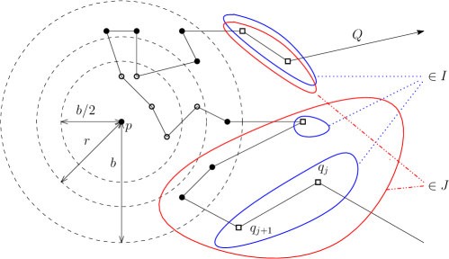
Figure 4 shows the pairs selected by Algorithm 1 into the $\theta$-guarding set $B$, for some $\theta\geq 1$, marked with polygonal red and blue bounds. The pairs within the red bound are avoidable, and the pairs within the blue bound are not. Two partial traversals $T_{1}$ and $T_{2}$ in $S_{B}$ that make the red bounded pairs avoidable (as in Definition 3.7) are marked by arrows.

$$F_{\delta/\theta}=\left(\begin{matrix}\includegraphics[width=143.09538pt]{avoidable}\end{matrix}\right)$$

Figure 4: Avoidable pairs from the $\theta$-guarding set $B$ (for some $\theta\geq 1$) are marked with red bound. Not avoidable pairs are marked with blue bound.

Lemma 3.8.

Given parameter $\theta\geq 1$ and the $\theta$-guarding set $B$. Let $B^{\prime}\subseteq B$ be the set of the avoidable pairs. Then $B\setminus B^{\prime}$ is a $\theta$-guarding set.

Proof.

The validity of the condition a) of Definition 3.1 for the set $B\setminus B^{\prime}$ is inherited from the set $B$. In order to prove the condition b), for the sake of contradiction let there exist a traversal $T$ of $P$ and $Q$ such that $T\cap\left(B\setminus B^{\prime}\right)=\emptyset$. Since by Lemma 3.4 the traversal $T$ of $P$ and $Q$ satisfies $T\cap B\neq\emptyset$, there exists $(i,j)\in T\cap B^{\prime}$, and we may assume that $(i,j)$ is the last such avoidable pair along $T$. Let $(i^{\prime},j^{\prime})\in B\setminus B^{\prime}$, $T_{1}$ and $T_{2}$ be respectively the pair in $B$ and two traversals from Definition 3.7 that make the pair $(i,j)$ avoidable.

We may assume that $(i^{\prime},j^{\prime})$ is in $B\setminus B^{\prime}$. To see this let $(i,j)=(i_{1},j_{1}),(i_{2},j_{2}),\ldots,(i_{\ell},j_{\ell})$ be the sequence of the pairs of indices, such that for all $m\in\{1,\ldots,\ell-1\}$:

1. the pair $(i_{m},j_{m})\in B^{\prime}$;

2. the pair $(i_{m+1},j_{m+1})$ makes the pair $(i_{m},j_{m})$ avoidable (from Definition 3.7); and

3. the pair $(i_{\ell},j_{\ell})\in B\setminus B^{\prime}$.

Such index $\ell$ has to exist, since it follows from Definition 3.7 and from the monotonicity of traversals, that $i_{1}<i_{2}<\ldots\leq n$ and $j_{1}<j_{2}<\ldots\leq n$. The partial traversals $T_{1}^{(\ell)}$ and $T_{2}^{(\ell)}$ from $(1,1)$ to $(i_{\ell},j_{\ell})$ given by Definition 3.7, that make the pair $(i_{\ell-1},j_{\ell-1})$ avoidable, satisfy the conditions of Definition 3.7 for the pair $(i,j)$ as well. We assign $(i^{\prime},j^{\prime})=(i_{\ell},j_{\ell})\in B\setminus B^{\prime}$, and thus it holds that $(i^{\prime},j^{\prime})\notin T$.

Let $(\hat{i},\hat{j})\in T\cap(T_{1}\cup T_{2})$ be the last such pair along $T$ (there has to exist at least one such pair, w.l.o.g let it be in $T_{1}$). We construct the traversal $T^{\prime}$ of $P$ and $Q$ out of the partial traversal of $T_{1}$ from $(1,1)$ to $(\hat{i},\hat{j})$ and the partial traversal of $T$ from $(\hat{i},\hat{j})$ to $(t,t)$. For the pairs $(i^{\prime\prime},j^{\prime\prime})\in T^{\prime}\cap T_{1}$ it holds by Definition 3.7 that $(i^{\prime\prime},j^{\prime\prime})\in S_{B}$. Thus $(T^{\prime}\cap T_{1})\cap B=\emptyset$, since $B\cap S_{B}=\emptyset$.

But since $T\cap B=\emptyset$, it is also $(T^{\prime}\cap T)\cap B=\emptyset$. Therefore for the traversal $T^{\prime}$ it holds that $T^{\prime}\cap B=\emptyset$. This contradicts the assumption that $B$ was the $\theta$-guarding set, and proves that the condition b) of Definition 3.1 holds. Thus $B\setminus B^{\prime}$ is a $\theta$-guarding set. ∎

3.2.4 Trimming the reachable area of a guarding set

Let $B$ be a $1$-guarding set for two curves $P$ and $Q$. We now want to modify $B$ to shrink the number of pairs while maintaining the guarding property. It turns out that we can do this if we relax the approximation quality of the guarding set (which we denoted with $\theta$). We perform this trimming in three phases:

1. Remove all avoidable pairs from $B$.

2. Trim the reachable area of $B$ row by row.

3. Trim the reachable area of $B$ column by column.

In the following, we describe the trimming operation on a single row. Consider a vertex $p_{i}$ of the curve $P$ and consider the intersection of $B$ with the row of the distance matrix associated with $p_{i}$. Let $I_{i}$ denote the set of intervals of the column indices that represent this intersection. We now apply Lemma 3.6 with parameter $b=d_{F}\!\left({P,Q}\right)$ to obtain a set of intervals $J_{i}$ that can be used to trim the reachable area of $B$ with respect to the $i$th row. Each interval in $J_{i}$ covers a set of intervals of $I_{i}$. Let $A_{i}$ be the subset of pairs of the $i$th row of which the column index is contained in an interval of $J_{i}$, but not contained in any interval of $I_{i}$. We call $A_{i}$ the filling pairs of the row. We now want to trim the reachable area $S_{B}$ defined by $B$ along the vertices of the reachability graph which correspond to pairs of $A_{i}$. For this we will remove all vertices of $B_{i}$ that are reachable from $A_{i}$ and add the pairs of $A_{i}$ to $B$. See Algorithm 2 for the pseudocode of this trimming operation. Figure 5 illustrates the process with an example. The trimming operation for a single column is analogous, except that we use $b=d_{F}\!\left({P,Q}\right)/2$ as a parameter to Lemma 3.6.

Data: guarding set $B$, row index $i$, value of $b>0$

Result: modified guarding set $B$

$I_{i}:=\{[j,j]~{}|~{}(i,j)\in B\}$;

  /* pairs of $B$ in the $i$th row */

1 Let $J_{i}$ be the set of intervals obtained from Lemma 3.6 using $I_{i}$ and $b=d_{F}\!\left({P,Q}\right)$;

$A_{i}:=S_{B}\cap\left\{(i,j)~{}|~{}j\in\left(\bigcup_{[j_{1},j_{2}]\in J_{i}}[j_{1},j_{2}]\setminus\bigcup_{[i_{1},i_{2}]\in I_{i}}[i_{1},i_{2}]\right)\right\}$;

  /* Compute filling pairs */

FIFO-Queue $\mathcal{Q}\leftarrow A_{i}$;

  /* find guarding pairs reachable from $A_{i}$ via BFS */

2 while $\mathcal{Q}\neq\emptyset$ do

3       $(i,j)\leftarrow\text{pop}(\mathcal{Q})$;

4       foreach $(i^{\prime},j^{\prime})\in\{(i+1,j),(i+1,j+1)\}$ do

5             if $(i^{\prime},j^{\prime})\in B\setminus\mathcal{Q}$  then

                  $B\leftarrow B\setminus\{(i^{\prime},j^{\prime})\}$ ;

                    /* remove them from $B$ */

6                  

7            else

8                   push($\mathcal{Q},(i^{\prime},j^{\prime})$);

9                  

10            

11      

$B\leftarrow B\cup A_{i}$;

  /* add pairs of $A_{i}$ to $B$ */

Algorithm 2 Trimming the reachable area for one row

$$F_{b}^{\text{before}}=\left(\begin{matrix}\ldots&&&&&\\ 0&0&\framebox{0}&\framebox{0}&\framebox{0}&\ldots\\ 0&\framebox{0}&1&1&\framebox{0}&\ldots\\ 0&1&1&\framebox{0}&0&\ldots\\ \framebox{0}&1&1&\framebox{0}&\framebox{0}&\ldots\\ 1&1&1&1&1&\ldots\end{matrix}\right)\hskip 28.45274ptF_{b/2}^{\text{after}}=\left(\begin{matrix}\ldots&&&&&\\ 0&0&\leavevmode\hbox to14.18pt{\vbox to14.18pt{\pgfpicture\makeatletter\hbox{\hskip 7.09111pt\lower-7.09111pt\hbox to0.0pt{\pgfsys@beginscope\pgfsys@invoke{ }\definecolor{pgfstrokecolor}{rgb}{0,0,0}\pgfsys@color@rgb@stroke{0}{0}{0}\pgfsys@invoke{ }\pgfsys@color@rgb@fill{0}{0}{0}\pgfsys@invoke{ }\pgfsys@setlinewidth{0.4pt}\pgfsys@invoke{ }\nullfont\hbox to0.0pt{\pgfsys@beginscope\pgfsys@invoke{ }{ {{}}\hbox{\hbox{{\pgfsys@beginscope\pgfsys@invoke{ }{{}{{{}}}{{}}{}{}{}{}{}{}{}{}{}{{}\pgfsys@moveto{6.89111pt}{0.0pt}\pgfsys@curveto{6.89111pt}{3.8059pt}{3.8059pt}{6.89111pt}{0.0pt}{6.89111pt}\pgfsys@curveto{-3.8059pt}{6.89111pt}{-6.89111pt}{3.8059pt}{-6.89111pt}{0.0pt}\pgfsys@curveto{-6.89111pt}{-3.8059pt}{-3.8059pt}{-6.89111pt}{0.0pt}{-6.89111pt}\pgfsys@curveto{3.8059pt}{-6.89111pt}{6.89111pt}{-3.8059pt}{6.89111pt}{0.0pt}\pgfsys@closepath\pgfsys@moveto{0.0pt}{0.0pt}\pgfsys@stroke\pgfsys@invoke{ } }{{{{}}\pgfsys@beginscope\pgfsys@invoke{ }\pgfsys@transformcm{1.0}{0.0}{0.0}{1.0}{-2.5pt}{-3.22221pt}\pgfsys@invoke{ }\hbox{{\definecolor{pgfstrokecolor}{rgb}{0,0,0}\pgfsys@color@rgb@stroke{0}{0}{0}\pgfsys@invoke{ }\pgfsys@color@rgb@fill{0}{0}{0}\pgfsys@invoke{ }\hbox{{0}} }}\pgfsys@invoke{\lxSVG@closescope }\pgfsys@endscope}}} \pgfsys@invoke{\lxSVG@closescope }\pgfsys@endscope}}} } \pgfsys@invoke{\lxSVG@closescope }\pgfsys@endscope{{{}}}{}{}\hss}\pgfsys@discardpath\pgfsys@invoke{\lxSVG@closescope }\pgfsys@endscope\hss}}\lxSVG@closescope\endpgfpicture}}&\leavevmode\hbox to14.18pt{\vbox to14.18pt{\pgfpicture\makeatletter\hbox{\hskip 7.09111pt\lower-7.09111pt\hbox to0.0pt{\pgfsys@beginscope\pgfsys@invoke{ }\definecolor{pgfstrokecolor}{rgb}{0,0,0}\pgfsys@color@rgb@stroke{0}{0}{0}\pgfsys@invoke{ }\pgfsys@color@rgb@fill{0}{0}{0}\pgfsys@invoke{ }\pgfsys@setlinewidth{0.4pt}\pgfsys@invoke{ }\nullfont\hbox to0.0pt{\pgfsys@beginscope\pgfsys@invoke{ }{ {{}}\hbox{\hbox{{\pgfsys@beginscope\pgfsys@invoke{ }{{}{{{}}}{{}}{}{}{}{}{}{}{}{}{}{{}\pgfsys@moveto{6.89111pt}{0.0pt}\pgfsys@curveto{6.89111pt}{3.8059pt}{3.8059pt}{6.89111pt}{0.0pt}{6.89111pt}\pgfsys@curveto{-3.8059pt}{6.89111pt}{-6.89111pt}{3.8059pt}{-6.89111pt}{0.0pt}\pgfsys@curveto{-6.89111pt}{-3.8059pt}{-3.8059pt}{-6.89111pt}{0.0pt}{-6.89111pt}\pgfsys@curveto{3.8059pt}{-6.89111pt}{6.89111pt}{-3.8059pt}{6.89111pt}{0.0pt}\pgfsys@closepath\pgfsys@moveto{0.0pt}{0.0pt}\pgfsys@stroke\pgfsys@invoke{ } }{{{{}}\pgfsys@beginscope\pgfsys@invoke{ }\pgfsys@transformcm{1.0}{0.0}{0.0}{1.0}{-2.5pt}{-3.22221pt}\pgfsys@invoke{ }\hbox{{\definecolor{pgfstrokecolor}{rgb}{0,0,0}\pgfsys@color@rgb@stroke{0}{0}{0}\pgfsys@invoke{ }\pgfsys@color@rgb@fill{0}{0}{0}\pgfsys@invoke{ }\hbox{{0}} }}\pgfsys@invoke{\lxSVG@closescope }\pgfsys@endscope}}} \pgfsys@invoke{\lxSVG@closescope }\pgfsys@endscope}}} } \pgfsys@invoke{\lxSVG@closescope }\pgfsys@endscope{{{}}}{}{}\hss}\pgfsys@discardpath\pgfsys@invoke{\lxSVG@closescope }\pgfsys@endscope\hss}}\lxSVG@closescope\endpgfpicture}}&\leavevmode\hbox to14.18pt{\vbox to14.18pt{\pgfpicture\makeatletter\hbox{\hskip 7.09111pt\lower-7.09111pt\hbox to0.0pt{\pgfsys@beginscope\pgfsys@invoke{ }\definecolor{pgfstrokecolor}{rgb}{0,0,0}\pgfsys@color@rgb@stroke{0}{0}{0}\pgfsys@invoke{ }\pgfsys@color@rgb@fill{0}{0}{0}\pgfsys@invoke{ }\pgfsys@setlinewidth{0.4pt}\pgfsys@invoke{ }\nullfont\hbox to0.0pt{\pgfsys@beginscope\pgfsys@invoke{ }{ {{}}\hbox{\hbox{{\pgfsys@beginscope\pgfsys@invoke{ }{{}{{{}}}{{}}{}{}{}{}{}{}{}{}{}{{}\pgfsys@moveto{6.89111pt}{0.0pt}\pgfsys@curveto{6.89111pt}{3.8059pt}{3.8059pt}{6.89111pt}{0.0pt}{6.89111pt}\pgfsys@curveto{-3.8059pt}{6.89111pt}{-6.89111pt}{3.8059pt}{-6.89111pt}{0.0pt}\pgfsys@curveto{-6.89111pt}{-3.8059pt}{-3.8059pt}{-6.89111pt}{0.0pt}{-6.89111pt}\pgfsys@curveto{3.8059pt}{-6.89111pt}{6.89111pt}{-3.8059pt}{6.89111pt}{0.0pt}\pgfsys@closepath\pgfsys@moveto{0.0pt}{0.0pt}\pgfsys@stroke\pgfsys@invoke{ } }{{{{}}\pgfsys@beginscope\pgfsys@invoke{ }\pgfsys@transformcm{1.0}{0.0}{0.0}{1.0}{-2.5pt}{-3.22221pt}\pgfsys@invoke{ }\hbox{{\definecolor{pgfstrokecolor}{rgb}{0,0,0}\pgfsys@color@rgb@stroke{0}{0}{0}\pgfsys@invoke{ }\pgfsys@color@rgb@fill{0}{0}{0}\pgfsys@invoke{ }\hbox{{0}} }}\pgfsys@invoke{\lxSVG@closescope }\pgfsys@endscope}}} \pgfsys@invoke{\lxSVG@closescope }\pgfsys@endscope}}} } \pgfsys@invoke{\lxSVG@closescope }\pgfsys@endscope{{{}}}{}{}\hss}\pgfsys@discardpath\pgfsys@invoke{\lxSVG@closescope }\pgfsys@endscope\hss}}\lxSVG@closescope\endpgfpicture}}&\ldots\\ 0&\leavevmode\hbox to14.18pt{\vbox to14.18pt{\pgfpicture\makeatletter\hbox{\hskip 7.09111pt\lower-7.09111pt\hbox to0.0pt{\pgfsys@beginscope\pgfsys@invoke{ }\definecolor{pgfstrokecolor}{rgb}{0,0,0}\pgfsys@color@rgb@stroke{0}{0}{0}\pgfsys@invoke{ }\pgfsys@color@rgb@fill{0}{0}{0}\pgfsys@invoke{ }\pgfsys@setlinewidth{0.4pt}\pgfsys@invoke{ }\nullfont\hbox to0.0pt{\pgfsys@beginscope\pgfsys@invoke{ }{ {{}}\hbox{\hbox{{\pgfsys@beginscope\pgfsys@invoke{ }{{}{{{}}}{{}}{}{}{}{}{}{}{}{}{}{{}\pgfsys@moveto{6.89111pt}{0.0pt}\pgfsys@curveto{6.89111pt}{3.8059pt}{3.8059pt}{6.89111pt}{0.0pt}{6.89111pt}\pgfsys@curveto{-3.8059pt}{6.89111pt}{-6.89111pt}{3.8059pt}{-6.89111pt}{0.0pt}\pgfsys@curveto{-6.89111pt}{-3.8059pt}{-3.8059pt}{-6.89111pt}{0.0pt}{-6.89111pt}\pgfsys@curveto{3.8059pt}{-6.89111pt}{6.89111pt}{-3.8059pt}{6.89111pt}{0.0pt}\pgfsys@closepath\pgfsys@moveto{0.0pt}{0.0pt}\pgfsys@stroke\pgfsys@invoke{ } }{{{{}}\pgfsys@beginscope\pgfsys@invoke{ }\pgfsys@transformcm{1.0}{0.0}{0.0}{1.0}{-2.5pt}{-3.22221pt}\pgfsys@invoke{ }\hbox{{\definecolor{pgfstrokecolor}{rgb}{0,0,0}\pgfsys@color@rgb@stroke{0}{0}{0}\pgfsys@invoke{ }\pgfsys@color@rgb@fill{0}{0}{0}\pgfsys@invoke{ }\hbox{{0}} }}\pgfsys@invoke{\lxSVG@closescope }\pgfsys@endscope}}} \pgfsys@invoke{\lxSVG@closescope }\pgfsys@endscope}}} } \pgfsys@invoke{\lxSVG@closescope }\pgfsys@endscope{{{}}}{}{}\hss}\pgfsys@discardpath\pgfsys@invoke{\lxSVG@closescope }\pgfsys@endscope\hss}}\lxSVG@closescope\endpgfpicture}}&1&1&\leavevmode\hbox to14.18pt{\vbox to14.18pt{\pgfpicture\makeatletter\hbox{\hskip 7.09111pt\lower-7.09111pt\hbox to0.0pt{\pgfsys@beginscope\pgfsys@invoke{ }\definecolor{pgfstrokecolor}{rgb}{0,0,0}\pgfsys@color@rgb@stroke{0}{0}{0}\pgfsys@invoke{ }\pgfsys@color@rgb@fill{0}{0}{0}\pgfsys@invoke{ }\pgfsys@setlinewidth{0.4pt}\pgfsys@invoke{ }\nullfont\hbox to0.0pt{\pgfsys@beginscope\pgfsys@invoke{ }{ {{}}\hbox{\hbox{{\pgfsys@beginscope\pgfsys@invoke{ }{{}{{{}}}{{}}{}{}{}{}{}{}{}{}{}{{}\pgfsys@moveto{6.89111pt}{0.0pt}\pgfsys@curveto{6.89111pt}{3.8059pt}{3.8059pt}{6.89111pt}{0.0pt}{6.89111pt}\pgfsys@curveto{-3.8059pt}{6.89111pt}{-6.89111pt}{3.8059pt}{-6.89111pt}{0.0pt}\pgfsys@curveto{-6.89111pt}{-3.8059pt}{-3.8059pt}{-6.89111pt}{0.0pt}{-6.89111pt}\pgfsys@curveto{3.8059pt}{-6.89111pt}{6.89111pt}{-3.8059pt}{6.89111pt}{0.0pt}\pgfsys@closepath\pgfsys@moveto{0.0pt}{0.0pt}\pgfsys@stroke\pgfsys@invoke{ } }{{{{}}\pgfsys@beginscope\pgfsys@invoke{ }\pgfsys@transformcm{1.0}{0.0}{0.0}{1.0}{-2.5pt}{-3.22221pt}\pgfsys@invoke{ }\hbox{{\definecolor{pgfstrokecolor}{rgb}{0,0,0}\pgfsys@color@rgb@stroke{0}{0}{0}\pgfsys@invoke{ }\pgfsys@color@rgb@fill{0}{0}{0}\pgfsys@invoke{ }\hbox{{0}} }}\pgfsys@invoke{\lxSVG@closescope }\pgfsys@endscope}}} \pgfsys@invoke{\lxSVG@closescope }\pgfsys@endscope}}} } \pgfsys@invoke{\lxSVG@closescope }\pgfsys@endscope{{{}}}{}{}\hss}\pgfsys@discardpath\pgfsys@invoke{\lxSVG@closescope }\pgfsys@endscope\hss}}\lxSVG@closescope\endpgfpicture}}&\ldots\\ 0&1&1&\leavevmode\hbox to14.18pt{\vbox to14.18pt{\pgfpicture\makeatletter\hbox{\hskip 7.09111pt\lower-7.09111pt\hbox to0.0pt{\pgfsys@beginscope\pgfsys@invoke{ }\definecolor{pgfstrokecolor}{rgb}{0,0,0}\pgfsys@color@rgb@stroke{0}{0}{0}\pgfsys@invoke{ }\pgfsys@color@rgb@fill{0}{0}{0}\pgfsys@invoke{ }\pgfsys@setlinewidth{0.4pt}\pgfsys@invoke{ }\nullfont\hbox to0.0pt{\pgfsys@beginscope\pgfsys@invoke{ }{ {{}}\hbox{\hbox{{\pgfsys@beginscope\pgfsys@invoke{ }{{}{{{}}}{{}}{}{}{}{}{}{}{}{}{}{{}\pgfsys@moveto{6.89111pt}{0.0pt}\pgfsys@curveto{6.89111pt}{3.8059pt}{3.8059pt}{6.89111pt}{0.0pt}{6.89111pt}\pgfsys@curveto{-3.8059pt}{6.89111pt}{-6.89111pt}{3.8059pt}{-6.89111pt}{0.0pt}\pgfsys@curveto{-6.89111pt}{-3.8059pt}{-3.8059pt}{-6.89111pt}{0.0pt}{-6.89111pt}\pgfsys@curveto{3.8059pt}{-6.89111pt}{6.89111pt}{-3.8059pt}{6.89111pt}{0.0pt}\pgfsys@closepath\pgfsys@moveto{0.0pt}{0.0pt}\pgfsys@stroke\pgfsys@invoke{ } }{{{{}}\pgfsys@beginscope\pgfsys@invoke{ }\pgfsys@transformcm{1.0}{0.0}{0.0}{1.0}{-2.5pt}{-3.22221pt}\pgfsys@invoke{ }\hbox{{\definecolor{pgfstrokecolor}{rgb}{0,0,0}\pgfsys@color@rgb@stroke{0}{0}{0}\pgfsys@invoke{ }\pgfsys@color@rgb@fill{0}{0}{0}\pgfsys@invoke{ }\hbox{{0}} }}\pgfsys@invoke{\lxSVG@closescope }\pgfsys@endscope}}} \pgfsys@invoke{\lxSVG@closescope }\pgfsys@endscope}}} } \pgfsys@invoke{\lxSVG@closescope }\pgfsys@endscope{{{}}}{}{}\hss}\pgfsys@discardpath\pgfsys@invoke{\lxSVG@closescope }\pgfsys@endscope\hss}}\lxSVG@closescope\endpgfpicture}}&0&\ldots\\ \framebox{0}&\framebox{0}&\framebox{0}&\framebox{0}&\framebox{0}&\ldots\\ 1&1&1&1&1&\ldots\end{matrix}\right)$$

Figure 5: The elements of a guarding set (marked with boxes) before (left) and after (right) applying of Algorithm 2 to the second row. The removed pairs are marked by circles

Lemma 3.9.

Let $B$ be a $1$-guarding set.

1. After the first phase of the algorithm, which removes all avoidable pairs, the modified set $B$ is a $1$-guarding set.

2. After the second phase of the algorithm, which applies the trimming operation to each row with $b=d_{F}\!\left({P,Q}\right)$, the modified set $B$ is a $2$-guarding set.

3. After the third phase of the algorithm, which applies the trimming operation to each column with $b=d_{F}\!\left({P,Q}\right)/2$, the modified set $B$ is a $4$-guarding set.

Proof.

The first part of the lemma follows directly from Lemma 3.8. We now prove the second part of the lemma statement. Condition (iii) of Lemma 3.6 ensures that any pair of a set $A_{i}$ added to $B$ corresponds to a pair of vertices $p\in P$ and $q\in Q$ with $d(p,q)\geq b/2=d_{F}\!\left({P,Q}\right)/2$. Indeed, the column indices of the pairs of $A_{i}$ are contained in intervals of $J_{i}$. Therefore, after the second phase, the modified set $B$ satisfies property (a) in the definition of guarding sets if we set $\theta=2$. Secondly, we argue that property (b) is not invalidated after the trimming operation was applied to a row. Let $B$ denote the guarding set before the trimming operation applied to the $i$th row and let $B^{\prime}$ denote the modifed guarding set after trimming. Clearly, the trimming operation does not add any avoidable pairs to $B$. Therefore we can assume that throughout the second phase no avoidable pairs are present.

Assume for the sake of contradiction that there exists a traversal $T$ that contains a pair of $B$, but does not contain a pair of $B^{\prime}$. Let $(i^{\prime},j^{\prime})$ be the first pair along $T$ that was removed from $B$ during the trimming operation and let $(i,j_{2})$ be a pair of $A_{i}$ that has a BFS-path to $(i^{\prime},j^{\prime})$. $T$ must contain a pair $(i,j_{1})$ in the $i$th row and this pair cannot be contained in an interval of $J_{i}$ (otherwise $T$ would contain a pair of $B^{\prime}$). Let $T_{1}$ be the partial traversal (path in $G$) of $T$ that starts in $(1,1)$ goes via $(i,j_{1})$ and ends in $(i^{\prime},j^{\prime})$. Since $(i^{\prime},j^{\prime})$ was the first vertex along $T$ in $B$, it follows that $T_{1}$ only visits vertices that are in $S_{B}$. Note that $i^{\prime}>i$ since the BFS only visits row indices strictly greater $i$. Since $A_{i}\subseteq S_{B}$, there must be a path $T_{2}$ in $G$ from $(1,1)$ via $(i,j_{2})$ to $(i^{\prime},j^{\prime})$ that only contains vertices of $S_{B}$. Now, condition (ii) of Lemma 3.6 implies that there must be a vertex $(i,j^{\prime\prime})$ in $B$, such that either $j_{1}<j^{\prime\prime}<j_{2}$ or $j_{2}<j^{\prime\prime}<j_{1}$. This implies that $(i,j^{\prime\prime})$ must be avoidable with respect to $B$. However, this contradicts the fact that $B$ does not contain any avoidable pairs. This proves (ii). The third part of the lemma follows by a symmetric argument applied to the columns. ∎

3.3 Bounding the complexity of the modified guarding set

Given set $B$ after the algorithm of Lemma 3.9. For every row of $B$ (presented as matrix) let the pairwise disjoint set of intervals $R_{i}\subseteq\{\left[j_{1},j_{2}\right]|j_{1}\leq j_{2}\in\mathbb{N},1\leq j_{1}\leq j_{2}\leq t\}$ be a set of intervals on $\{1,\ldots,t\}$ of minimal size, such that for any $1\leq j^{\prime}\leq t$ there exist $j_{1}$ and $j_{2}$ with $j^{\prime}\in[j_{1},j_{2}]\in R_{i}$ if and only if $(i,j^{\prime})\in B$. We can analogously define such pairwise disjoint sets $C_{j}$ over the columns of $B$.

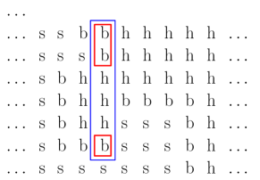
Lemma 3.6 implies that for every row $i$ there is a set of pairwise disjoint intervals $J_{i}$ constructed by line 2 of Algorithm 2, with $|J|\leq c+1$. Algorithm 2 takes into $B$ only the pairs that belong to the subsets of the intervals of $J_{i}$ that were in $S_{B}$ too. But since the pairs $(i,j)\in H_{B}$ such that $j\in[j_{1},j_{2}]\in J_{i}$ have the property that any traversal using these pairs has to contain a pair in $B$ prior to $(i,j)$, we could have added such pairs too into $B$ and then it would be $J_{i}=R_{i}$. Since we took only its subsets, it holds that for every $[j_{1},j_{2}]\in R_{i}$ there is $[j_{3},j_{4}]\in J_{i}$ with $j_{3}\leq j_{1}\leq j_{2}\leq j_{4}$. By counting all intervals of $R_{i}$ that are subset of one interval from $J_{i}$ as one, we say that all such intervals $R_{i}$ build one extended group of consecutive pairs within $i$th row. It follows that there are at most $c+1$ extended groups within $i$-th row. This process gets repeated over columns as well. See Figure 6 for an illustration.

Figure 6: The pairs of the guarding set $B$ (red) and its extended group (blue) within one column. The pairs denoted with s, b, and h are from $S_{B}$, $B$ and $H_{B}$ respectively

We have to note that the filling pairs added into $B$ also imply the removal of a pair in $B$ that lies in the same row but with higher column index, except possibly for the last pair in the row. This can happen at most once per row, adding one pair (and one extended group) to the row. We obtain the following lemma.

Lemma 3.10.

In the guarding set produced by Algorithm 1 and modifed by the algorithm of Lemma 3.9, there are at most $c+1$ extended groups within a column, and $c+2$ extended groups within a row.

To finally bound the complexity of our guarding set by Lemma 3.12, we show first Lemma 3.11.

Lemma 3.11.

For the guarding set produced by Algorithm 1 and after every phase of algorithm of Lemma 3.9 the following invariant holds: for every pair $(i,j)\in B$ there exists a pair $(i^{\prime},j^{\prime})\in S_{B}$ such that $((i^{\prime},j^{\prime}),(i,j))\in E$.

Proof of Lemma 3.11.

We call the pair $(i^{\prime},j^{\prime})$ the predecessor pair. The construction of the guarding set $B$ Algorithm 1 guarantees that a pair $(i,j)$ is added into $B$ if it is visited over an edge $((i^{\prime},j^{\prime}),(i,j))\in E$, where $(i^{\prime},j^{\prime})\notin B$. Thus $((i^{\prime},j^{\prime})\in S_{B}$ as claimed.

The first phase of the algorithm of Lemma 3.9 removes the avoidable pairs from $B$, thus for the pairs that remain in $B$ the invariant holds. The second phase runs Algorithm 2 upon a row and adds into $B$ only pairs which were already in $S_{B}$, thus have also a predecessor in $S_{B}$. For every pair $(i^{\prime},j^{\prime})$ which was in $S_{B}$ before and is in $H_{B}$ after Algorithm 2 it holds that the BFS passes it and then visits and subsequently removes the pairs from $B$. Therefore the invariant remains valid for the pairs that remain in $B$, as for the pairs that were already in $B$ their predecessors remain in $S_{B}$, so their status is not changed. The third phase is equivalent to the second one, and the invariant remains valid. ∎

Lemma 3.12.

The set $B$ obtained by the algorithm of Lemma 3.9 is a $4$-guarding set, containing at most $(3c+4)\cdot t$ pairs.

Proof.

For every pair $(i,j)\in B$ one of the following holds true:

1. the index $j$ is the smallest index of an extended group over the $i$th row;

2. the index $i$ is the smallest index of an extended group over the $j$th column;

3. none of the above.

We argue that if neither i) nor ii) holds true, then it must be that $i-1$ is the smallest index of an extended group over the $j$th column. Indeed, note that if neither i) nor ii) holds true, then $(i-1,j)$ and $(i,j-1)$ are part of an extended group and such groups can only contain pairs of $B$ or $H_{B}$. Therefore, the pair $(i-1,j-1)$ must be in $S_{B}$ because Lemma 3.11 implies that $(i,j)$ must have an ingoing edge from a pair in $S_{B}$. Now, since pairs of $S_{B}$ and $H_{B}$ cannot be directly connected by an edge of $G$, it must be that $(i-1,j)$ and $(i,j-1)$ are both in $B$. Thus, $i-1$ is the smallest index of an extended group over the $j$th column.

We charge elements of $B$ of type i) and of type ii) to their respective extended intervals. We charge elements of type iii) it to their extended interval over the column. Thus, extended intervals in the column are charged at most twice. By Lemma 3.10 we have at most $(c+1)$ extended intervals per column and at most $(c+2)$ extended intervals per row. This implies that altogether $|B|\leq(3c+4)\cdot t$, as claimed. ∎

Lemma 3.2 and Lemma 3.12 imply the correctness of Theorem 1.1. The proof of Theorem 1.2 is analogous to the proof of Theorem 1.1, while Lemma 2.2 and Lemma 3.2 are replaced by Lemma 2.3 and Lemma 3.3, respectively. The rest of the proof can be taken verbatim.

4 Lower bounds

4.1 Definitions

Related similarity measure between two curves to the discrete Fréchet distance is dynamic time warping. It considers the sum of the used distances in the traversal (instead the maximum one). Formally, for two curves $P$ and $Q$ from $\mathbb{R}^{d}$, we define:

$$d_{DTW}\!\left({P,Q}\right)=\min_{T\in\mathcal{T}}\sum_{(i,j)\in T}\|p_{i}-q_{j}\|.$$ (10)

For the continuous Fréchet distance, let again $P=\{p_{1},\ldots,p_{t}\}$ and $Q=\{q_{1},\ldots,q_{t}\}$ be two curves from $\mathbb{R}^{d}$. Let $\pi:[0,1]\rightarrow P$ and $\tau:[0,1]\rightarrow Q$ be two functions on $[0,1]$ such that $\pi(0)=p_{1}$, $\pi(1)=p_{t}$, $\tau(0)=q_{1}$ and $\tau(1)=q_{t}$, and such that $\pi$ and $\tau$ are monotone on $P$ and $Q$ respectively. Let $\mathcal{H}$ denote the set of continuous and increasing functions $f:[0,1]\rightarrow[0,1]$ with the property that $f(0)=0$ and $f(1)=1$. For two given curves $P$ and $Q$ and respective functions $\pi$ and $\tau$, their (continuous) Fréchet distance is defined as

$$d_{F}\!\left({P,Q}\right)=\inf_{f\in\mathcal{H}}\;\max_{t\in[0,1]}\|Q(\tau(f(t)))-P(\pi(t))\|$$ (11)

and the function $f$ that reaches the value $\delta=d_{F}\!\left({P,Q}\right)$ is called matching from $P$ to $Q$ with cost $\delta$.

4.2 c-packed curves

We prove the correctness of Theorem 1.3 for the discrete and the continuous Fréchet distance, as well as for the dynamic time warping distance.

Proof of Theorem 1.3 for the discrete Fréchet distance.

Let the curves $P$ and $Q$ be from $\mathbb{R}^{2}$. Let the curve $P=\{p_{1},\ldots,p_{2t+1}\}$ be the line segment $\overline{p_{1}p_{2t+1}}$, while the vertices $p_{2},\ldots,p_{2t}$ are uniformly distributed on $P$, i.e. $\|p_{i+1}-p_{i}\|=\|p_{i}-p_{i-1}\|$ for all $i\in\{2,\ldots,2t\}$. Let $Q=\{q_{1},\ldots,q_{2t+1}\}$ be composed by two line segments $\overline{q_{1}q_{t+1}}$ and $\overline{q_{t+1}q_{2t+1}}$, and the vertices $q_{2},\ldots,q_{2t}$ are uniformly distributed on $Q$, i.e. $\|q_{j+1}-q_{j}\|=\|q_{j}-q_{j-1}\|$ for all $j\in\{2,\ldots,2t\}$. Let $p_{1}=q_{1}$ and $p_{2t+1}=q_{2t+1}$ and let $\angle q_{t+1}q_{1}p_{2t+1}=\alpha$ (as shown in Figure 7).

Figure 7: Lower bound for the discrete Fréchet distance case for $c$-packed curves

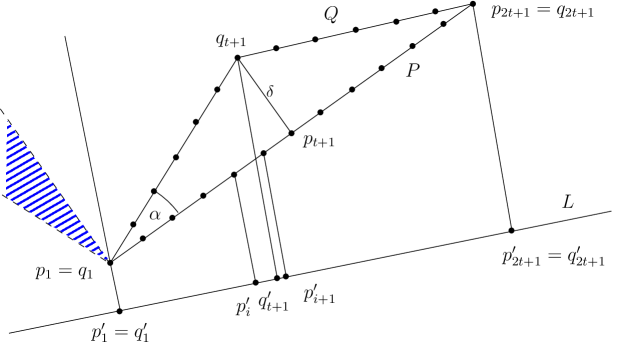
The curves $P$ and $Q$ are $c$-packed for any constant $c\geq 2$. Let $|Q|=2$, then it holds that $|P|=2\cdot|\cos\alpha|$ and for both discrete and continuous Fréchet distance it holds that $\delta=d_{F}\!\left({P,Q}\right)=|\sin\alpha|$.

Let the straight line $L$ support the unit vector u, which is chosen uniformly at random on the unit hypersphere, and let $P$ and $Q$ be projected to $L$. Observe that the discrete Fréchet distance of $P$ and $Q$ is realized by the pair $(t+1,t+1)$ in the traversal of $P$ and $Q$, thus $\|p_{t+1}-q_{t+1}\|=d_{F}\!\left({P,Q}\right)=\delta$. The vertex $q_{t+1}\in Q$ is projected to $q^{\prime}_{t+1}$ and $q^{\prime}_{t+1}$ lies either within $P^{\prime}$ or outside of it.

If it is inside ($q^{\prime}_{t+1}\in P^{\prime}$), and thus in one of the $2t$ line segments $\overline{p^{\prime}_{i}p^{\prime}_{i+1}}$ for some $i\in\{1,\ldots,2t\}$, then the distance of $q^{\prime}_{t+1}$ to its matched vertex $p^{\prime}_{x}\in P^{\prime}$ is at most

$$\|q^{\prime}_{t+1}-p^{\prime}_{x}\|\leq\frac{|P^{\prime}|}{2t}\leq\frac{|P|}{2t}=\frac{|\cos\alpha|}{t}.$$

Therefore it holds that

$$q^{\prime}_{t+1}\in P^{\prime}\Rightarrow d_{F}\!\left({P^{\prime},Q^{\prime}}\right)\leq\frac{|\cos\alpha|}{t}\leq\frac{1}{t}.$$

The event $q^{\prime}_{t+1}\in P^{\prime}$ occurs with probability at least $1-\alpha/\pi$, i.e. when the perpendicular line to $L$ is not parallel to some straight line laying in $\angle q_{t+1}q_{1}p_{2t+1}=\alpha$ and including $q_{1}$ (tiled area in Figure 7). Then it holds that

$$\text{Pr}\left[\frac{d_{F}\!\left({P,Q}\right)}{d_{F}\!\left({P^{\prime},Q^{\prime}}\right)}\geq|\sin\alpha|\cdot t\right]\geq 1-\frac{\alpha}{\pi}.$$

For $\alpha\in[0,1]$ it holds that $|\sin\alpha|\geq\alpha-\alpha^{3}/3!\geq\frac{5}{6}\alpha$, thus for $\gamma=\alpha/\pi$ is for $\gamma\in(0,1/\pi)$:

$$\text{Pr}\left[\frac{d_{F}\!\left({P,Q}\right)}{d_{F}\!\left({P^{\prime},Q^{\prime}}\right)}\geq\frac{5\pi\gamma}{6}\cdot t\right]\geq 1-\gamma$$

This proves the correctness of the theorem.

∎

Proof of Theorem 1.3 for the continuous Fréchet distance.

For the continuous case it holds that if $q^{\prime}_{t+1}\in P^{\prime}$, then $P^{\prime}=Q^{\prime}$ and $d_{F}\!\left({P^{\prime},Q^{\prime}}\right)=0$. Thus it holds that

$$\text{Pr}\left[\frac{d_{F}\!\left({P,Q}\right)}{d_{F}\!\left({P^{\prime},Q^{\prime}}\right)}\geq t\right]\geq\text{Pr}\left[d_{F}\!\left({P^{\prime},Q^{\prime}}\right)=0\right]\geq 1-\alpha/\pi$$

for any constant $\alpha\in(0,1)$. Thus the continuous Fréchet distance will be reduced at least by a factor of $t$ with probability at least $1-\gamma$, where $\gamma=\alpha/\pi$ and $\gamma\in(0,1/\pi)$. ∎

Proof of Theorem 1.3 for the dynamic time warping distance.

For the curves $P$ and $Q$ it holds that

$$d_{DTW}\!\left({P,Q}\right) = \sum_{i=1}^{2t+1}\|p_{i}-q_{i}\|=2\cdot\left(\sum_{i=2}^{t}\|p_{i}-q_{i}\|\right)+\|p_{t+1}-q_{t+1}\|$$

$$= 2\cdot\left(\sum_{i=1}^{t}\|p_{i+1}-q_{i+1}\|\right)-\|p_{t+1}-q_{t+1}\|=2\cdot\left(\sum_{i=1}^{t}\frac{i\cdot|\sin\alpha|}{t}\right)-|\sin\alpha|$$

$$= t\cdot|\sin\alpha|$$

For the projection curves it holds that with the probability $1-\alpha/\pi$ that (analogously to the discrete Fréchet distance case):

$$d_{DTW}\!\left({P^{\prime},Q^{\prime}}\right) = \min_{T\in\mathcal{T^{\prime}}}\sum_{(i,j)\in T}\|p^{\prime}_{i}-q^{\prime}_{j}\|$$

where $\mathcal{T^{\prime}}$ is the set of all traversals of $P^{\prime}$ and $Q^{\prime}$.

Let the set of the pairs $T^{\prime}$ be defined, such that for $1\leq j\leq 2t+1$, the pair $(i,j)\in T^{\prime}$ iff $\|p^{\prime}_{i}-q^{\prime}_{j}\|$ is minimal over all $1\leq i\leq 2t+1$. Such set $T^{\prime}$ is a traversal of $P^{\prime}$ and $Q^{\prime}$. This is shown by induction, since $p_{1}=q_{1}$ and $p_{2t+1}=q_{2t+1}$. Let the pair $(i,j)$ be in $T^{\prime}$. Then the closest vertex of $P^{\prime}$ to the vertex $q^{\prime}_{j+1}$ has to be either $p^{\prime}_{i}$ or $p^{\prime}_{i+1}$. The other ones (either with smaller or greater index) cannot be the closest ones to $q^{\prime}_{j+1}$ because of the order of the vertices on $P^{\prime}$ and $Q^{\prime}$. Thus the pair $(i,j)\in T^{\prime}$ is followed either by $(i+1,j+1)$ or $(i,j+1)$ (the possibility of $(i+1,j)$ is excluded, since we choose exactly one matched vertex for each $j$, $1\leq j\leq 2t+1$), and $T^{\prime}\in\mathcal{T}^{\prime}$ is a traversal.

Therefore it holds that

$$d_{DTW}\!\left({P^{\prime},Q^{\prime}}\right) \leq \sum_{(i,j)\in T^{\prime}}\|p^{\prime}_{i}-q^{\prime}_{j}\|\leq\frac{1}{2}\sum_{(i,j)\in T^{\prime}}\|p^{\prime}_{i}-p^{\prime}_{i+1}\|$$

$$\leq \frac{1}{2}\sum_{i=2}^{2t}\|p^{\prime}_{i}-p^{\prime}_{i+1}\|\leq\frac{1}{2}\cdot|P^{\prime}|\leq\frac{1}{2}\cdot|P|=|\cos\alpha|\leq 1$$

with the probability $1-\alpha/\pi$. Thus

$$\text{Pr}\left[\frac{d_{DTW}\!\left({P,Q}\right)}{d_{DTW}\!\left({P^{\prime},Q^{\prime}}\right)}\geq|\sin\alpha|\cdot t\right]\geq 1-\frac{\alpha}{\pi}.$$

By repeating the analysis of Theorem 1.3 for the discrete Fréchet distance we obtain that the dynamic time warping distance will be reduced at least by a factor of $5\pi\gamma t/6$ with probability at least $1-\gamma$, for any $\gamma\in(0,1/\pi)$. ∎

4.3 General case curves

If the curves $P$ and $Q$ are not $c$-packed, for any constant $c\geq 2$, then the ratio of the continuous Fréchet distances between $P$ and $Q$ and their projection curves $P^{\prime}$ and $Q^{\prime}$ can be at least linear in $t$, as claimed by Theorem 4.1. This event can happen with probability 1. We claim the same bound for the discrete Fréchet distance.

Theorem 4.1.

There exist the curves $P=\{p_{1},\ldots,p_{t}\}$ and $Q=\{q_{1},\ldots,q_{t}\}$, such that if $P^{\prime}$ and $Q^{\prime}$ respectively are their projections to the one-dimensional space that supports the unit vector chosen uniformly at random on the unit hypersphere, then it holds that

$$\frac{d_{F}\!\left({P,Q}\right)}{d_{F}\!\left({P^{\prime},Q^{\prime}}\right)}\geq f(t),$$

where $f(t)\in\Omega(t)$.

Proof of Theorem 4.1 for the continuous Fréchet distance.

We denote with $P_{k}$ the star-like closed curve with $2k+1$ vertices, defined as $P_{k}=\{p_{1},p_{0},p_{2},$ $p_{0},\ldots,p_{k},p_{0},p_{k+1}\}$. Let $p_{i}=(r_{i},\theta_{i})$ in polar coordinates be defined as $p_{0}=(0,0)$, $p_{k+1}=p_{0}$ and $p_{i}=(1,2\cdot(i-1)\cdot\pi/k)$ for $1\leq i\leq k$. Let $P=P_{k}$ and $Q=P_{k+1}$, and let $k$ be even. To have the same complexity for $P$ and $Q$ we can add two more points $p_{1}$ at the end, thus $t=2k+3$. We denote the indices of the curve $Q$ with $q_{j}$, $0\leq j\leq k+2$. Figure 8 shows the curves $P$ and $Q$ for $k=12$ (in full blue and dotted red line respectively).

Figure 8: Two curves $P$ and $Q$ with parameter $k=12$

The Fréchet distance between the curves $P$ and $Q$ is $d_{F}\!\left({P,Q}\right)=1/\left(2\cdot\cos(\pi/(k+1))\right)$. To show this, let $M$ be the matching of the points of $P$ and $Q$ that realizes the Fréchet distance. The curve $Q$ has one more “ray” of the star to be traversed. The “rays” $\overline{p_{0},p_{1},p_{0}}$ and $\overline{q_{0},q_{1},q_{0}}$ are equal, they are matched by $M$ at distance 0; and the “rays” $\overline{p_{0},p_{i},p_{0}}$ and $\overline{q_{0},q_{i},q_{0}}$ for $1\leq i\leq k/2$, and $\overline{p_{0},p_{i},p_{0}}$ and $\overline{q_{0},q_{i+1},q_{0}}$ for $1\leq i\leq k/2+2$ are pairwise matched by $M$ at distance smaller than $\pi/(k+1)$. There remain two consecutive “rays” $\overline{q_{0}q_{j}q_{0}}$ and $\overline{q_{0}q_{j+1}q_{0}}$ that have to be matched by the matching $M$ to $\overline{p_{0}p_{j}p_{0}}$, with $j=k/2+1$. The point $\tilde{p}$ with coordinates $\left(1/\left(2\cdot\cos(\pi/(k+1))\right),\pi\right)$ is the intersection of a bisector of $\overline{q_{0}q_{j}}$ with $\overline{p_{0}p_{j}}$. Such point $\tilde{p}$ matches the subcurve of $Q$ between the vertices $\{q_{k/2+1},q_{0},q_{k/2+2}\}$, thus the matching $M$ is completely described, and the Fréchet distance realized by $M$ is $\|q_{k/2+1}-\tilde{p}\|=\|p_{0}-\tilde{p}\|=1/\left(2\cdot\cos(\pi/(k+1))\right)$, as claimed. It holds that $d_{F}\!\left({P,Q}\right)>1/2$ for any $k\geq 2$.

We notice that between every two lines $\overline{q_{0}q_{j}}$ and $\overline{q_{0}q_{j+1}}$ there has to be one line $\overline{p_{0}p_{i}}$ (the opposite does not have to hold). Thus the distance between $p_{i}$ and any of its neighboring $q_{j}$ and $q_{j+1}$ is at most $\max\{\|q_{j}-p_{i}\|,\|q_{j+1}-p_{i}\|\}\leq\|q_{j+1}-q_{j}\|\leq 2\pi/(k+1)$, since $p_{i}$ is on the circular arc between $q_{j}$ and $q_{j+1}$.

If we now project the curves $P$ and $Q$ to the straight line that supports the unit vector u, with u chosen uniformly at random on the unit hypersphere, let $P^{\prime}=\{p^{\prime}_{1},p^{\prime}_{0},\ldots,p^{\prime}_{k},p^{\prime}_{0},p^{\prime}_{k+1}\}$ and $Q=\{q^{\prime}_{1},q^{\prime}_{0},\ldots,q^{\prime}_{k+1},q^{\prime}_{0},q^{\prime}_{k+2}\}$ be their projections respectively. The line $\overline{q_{0}q^{\prime}_{0}}$ satisfies one of the following two cases:

1. $\overline{q_{0}q^{\prime}_{0}}\|\overline{q_{0}q_{j}}$ for some $1\leq j\leq k+1$, or

2. $\overline{q_{0}q^{\prime}_{0}}$ lies between $\overline{q_{0}q_{j}}$ and $\overline{q_{0}q_{j+1}}$ for some $1\leq j\leq k+1$.

Then in the first case, since $k$ is even, the straight line $\overline{q_{0}q^{\prime}_{0}}$ lies between $\overline{q_{0}q_{(j+k/2)\mod(k+1)}}$ and $\overline{q_{0}q_{1+(j+k/2)\mod(k+1)}}$ (through the two vertices on the opposite side of the star). Therefore, we may only consider the second case.

The projected curves $P^{\prime}$ and $Q^{\prime}$ can be matched by a matching $M^{\prime}$ as follows: let $p_{i}$ be the vertex of $P$ that lies between $\overline{q_{0}q_{j}}$ and $\overline{q_{0}q_{j+1}}$ from the case definition. Let $p^{\prime}_{i}$ be its projection. Then let the subcurves $\{p^{\prime}_{0},p^{\prime}_{i},p^{\prime}_{0}\}$ and $\{q^{\prime}_{0},q^{\prime}_{j},q^{\prime}_{0},q^{\prime}_{j+1},q^{\prime}_{0}\}$ be matched to each other by matching $M^{\prime}$. For the rest of the curves let $\{p^{\prime}_{0},p^{\prime}_{i+\ell},p^{\prime}_{0}\}$ and $\{p^{\prime}_{0},p^{\prime}_{i-\ell},p^{\prime}_{0}\}$ be matched to $\{q^{\prime}_{0},q^{\prime}_{j+1+\ell},q^{\prime}_{0}\}$ and $\{q^{\prime}_{0},q^{\prime}_{j-\ell},q^{\prime}_{0}\}$ respectively, where $1\leq i-\ell$ or $i+\ell\leq k+1$.

Let $M^{\prime}(p^{\prime}_{i})$ be the point on $Q^{\prime}$ that is matched to $p^{\prime}_{i}$. Let $\overline{M}(p^{\prime}_{i})$ be the point on $Q$ such that $M^{\prime}(p^{\prime}_{i})$ is its projection on $L$. If we denote with $\alpha_{i}$ the angle between the vector $\overline{M}(p^{\prime}_{i})-p_{i}$ and the unit vector u, then for the Fréchet distance between the projections $P^{\prime}$ and $Q^{\prime}$ (that lay in the one-dimensional space) it holds that

$$d_{F}\!\left({P^{\prime},Q^{\prime}}\right) \leq \max_{1\leq i\leq k}\{\|M^{\prime}(p^{\prime}_{i})-p^{\prime}_{i}\|\}=\max_{1\leq i\leq k}\{\|\overline{M}(p^{\prime}_{i})-p_{i}\|\cdot|\cos\alpha_{i}|\}$$

$$\leq \max_{1\leq i\leq k}\{\|\overline{M}(p_{i})-p_{i}\|\}\leq\frac{2\pi}{k}$$

Therefore by projecting the curves $P$ and $Q$ to any straight line the Fréchet distance between the curves will be diminished at least by the factor

$$\frac{d_{F}\!\left({P^{\prime},Q^{\prime}}\right)}{d_{F}\!\left({P,Q}\right)}<\frac{2\pi}{k}\cdot 2=\frac{4\pi}{k}.$$

This yields the claimed linear lower bound, since $k=(t-3)/2$ and proves the theorem with $f(t)=(t-3)/(8\pi)$. ∎

Proof of Theorem 4.1 for the discrete Fréchet distance.

The lower bound given by Theorem 4.1 holds also for the discrete Fréchet distance, with $f(t)=(t-5)/(16\pi)$. We adapt the curves $P$ and $Q$ from the proof for the continuous Fréchet distance as follows. Let us add to each “ray” $\overline{p_{0}p_{i}p_{0}}$ of the curve $P_{k}$ the vertices $\hat{p}_{i}$ (i.e. the “ray” becomes $\overline{p_{0}\hat{p}_{i}p_{i}\hat{p}_{i}p_{0}}$), with polar coordinates $\hat{p}_{i}=\left(1/\left(2\cdot\cos(\pi/(k+1)\right),\right.$ $\left.2\cdot(i-1)\cdot\pi/k\right)$. The curve $P_{k}$ contains now $4k+1$ vertices and $t=4k+5$. The rest of the construction and analysis can be used verbatim. ∎

5 Experiments

We performed the preliminary experiments on the dataset of the 6th ACM SIGSPATIAL GISCUP 2017 competition. Their dataset $\mathcal{D}$ contains 20199 realistic polygonal curves from $\mathbb{R}^{2}$, with complexities between 9 and 767. We have repeated the following procedure for 504 pairs of curves of $\mathcal{D}$ selected uniformly at random. For each pair of curves (or their subcurves) the projection line was sampled $r=1000$ times. We observed the obtained distribution of the distortion $c$ of the discrete Fréchet distance.

1. We calculated the distortion $c=d_{F}\!\left({P^{\prime},Q^{\prime}}\right)/d_{F}\!\left({P,Q}\right)$ for the whole curves.

2. We observed the prefix curves $P_{\ell}=\{p_{1},\ldots,p_{\ell}\}$ and $Q_{\ell}=\{q_{1},\ldots,q_{\ell}\}$ of $P$ and $Q$ respectively, with complexity $\ell$ equal 10, or to the multiples of $50$. The distortion $c=d_{F}\!\left({P^{\prime}_{\ell},Q^{\prime}_{\ell}}\right)/d_{F}\!\left({P_{\ell},Q_{\ell}}\right)$ is calculated.

3. For every prefix length $\ell$ we chose at random subcurves of $P$ and $Q$ of complexity $\ell$, defined by $\ell$ consecutive vertices of $P$ and $Q$ respectively. Let these curves be $P_{\ell,r}$ and $Q_{\ell,r}$. We calculated the distortion $c=d_{F}\!\left({P^{\prime}_{\ell,r},Q^{\prime}_{\ell,r}}\right)/d_{F}\!\left({P_{\ell,r},Q_{\ell,r}}\right)$.

This yielded 4286 pairs of (sub)curves.

Figure 9: The curves $(9392,9836)$ from the dataset $\mathcal{D}$ (left). The cumulative probability distribution of the distortion $c$, over all tested subcurves of the input pair of curves $(9392,9836)$ from $\mathcal{D}$ (right).

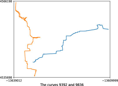
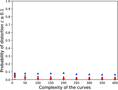
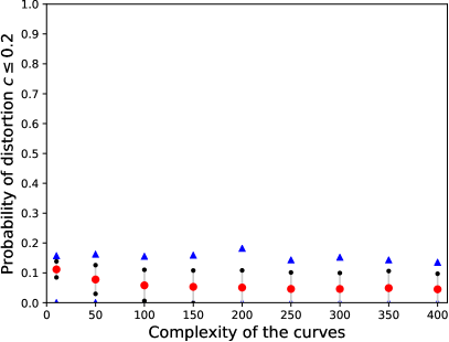
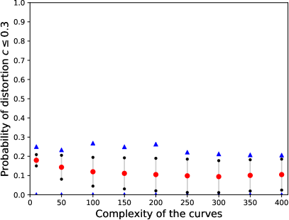
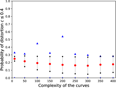
E.g. we observe the pair of the curves $P$ and $Q$ (numbered 9382 and 9836) shown in Figure 9 (left) with complexities 308 and 357 respectively. For these curves and their subcurves, the cumulative probability distributions of $c$ were calculated, over the set of results of 1000 sampled runs. We notice that the Fréchet distance of the curves $P$ and $Q$ in Figure 9 (or their subcurves) is not dominated by one pair of vertices, and varies upon which parts of the curves are observed. For all pairs of subcurves of $P$ and $Q$ and their respective projections $P^{\prime}$ and $Q^{\prime}$ we may assume that for any $\gamma\in(0,1)$ it is

$$\text{Pr}\left[\frac{d_{F}\!\left({P^{\prime},Q^{\prime}}\right)}{d_{F}\!\left({P,Q}\right)}\leq\gamma\right]\leq\gamma.$$ (12)

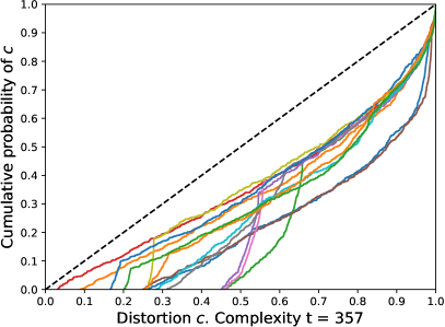
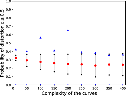
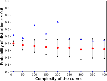
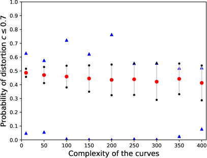
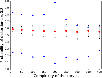
Indeed, when the cumulative probability distribution of the distortion $c$ is observed over all tested pairs of curves (Figure 10, upper left), the mean and the standard deviation of the distortions obtained by our experiments for a given threshold $\gamma\in\{0.1,0.2,0.3,0.4,0.5,0.6,0.7,0.8,$ $0.9\}$, suggest that for the realistic input curves $P$ and $Q$ the assumption of Equation (12) holds with high probability. The outlying maxima occur for the curves whose shape is similar to the curves from the proof of Theorem 1.3, and thus strongly conditioned.

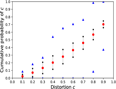
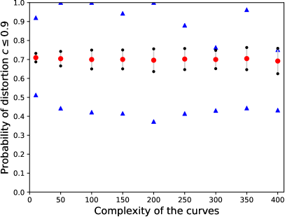
Furthermore, it seems that the distortion of the discrete Fréchet distance is bounded by a constant (with high probability), and that it does not depend on the complexity $t$ of the input curves, as suggested by Figure 10 and Figure 11.

Figure 10: The cumulative probability distribution of the distortion (upper left). The remaining subfigures show for a given threshold $\gamma$ of the distortion $c$, the cumulative probability $\text{Pr}[c\leq\gamma]$ as a function of the complexity $t$ of the curves, for $t\in\{10,50,100,150,200,250,300,350,400\}$. The means $\mu$ of the values denoted by red circles. The intervals $[\mu-\sigma,\mu+\sigma]$ denoted by black dots, where $\sigma$ is the standard deviation. The minima and maxima denoted by blue triangles. Continued in Figure 11

Figure 11: Figure 10 continued.

6 Conclusions

We studied the behavior of the discrete Fréchet distance between two polygonal curves under projections to a random line. Our results show that in the worst case and under reasonable assumptions, the discrete Fréchet distance between two polygonal curves of complexity $t$ in ${\rm I\!R}^{d}$, where $d\in\{2,3,4,5\}$, degrades by a factor linear in $t$ with constant probability. One can see this as a negative result, since we hoped that the Fréchet distance would be more robust under such projections. We also performed some preliminary experiments on the dataset of the 6th ACM SIGSPATIAL GISCUP 2017 competition (as seen in Section 5). The cumulative probability distribution of the distortion $c=d_{F}\!\left({P^{\prime},Q^{\prime}}\right)/d_{F}\!\left({P,Q}\right)$ (Figure 10, first row, left) suggests that for realistic input curves we can expect that $\text{Pr}\left[c\leq\gamma\right]\leq\gamma$. This holds independently of the complexity $t$ of the input curves, as illustrated by Figure 11 (first row, right) for the given threshold $\gamma=0.5$. This implies that with probability of at least $0.5$ we expect that the discrete Fréchet distance will be reduced at most by a factor 2 when projected to a line chosen uniformly at random, independently of the input complexity. These results stand in stark contrast with our lower bounds. They indicate that highly distorted projections happen very rarely in practice, and only for strongly conditioned input curves.

Acknowledgements.

We thank Kevin Buchin for useful discussions on the topic of this paper.

References

- [1] A. Abboud, A. Backurs, and V. V. Williams. Quadratic-time hardness of LCS and other sequence similarity measures. CoRR, abs/1501.07053, 2015.
- [2] P. Afshani and A. Driemel. On the complexity of range searching among curves. In Proceedings of the 29th ACM-SIAM Symposium on Discrete Algorithms, SODA, pages 898–917, 2018.
- [3] P. K. Agarwal, R. Ben Avraham, H. Kaplan, and M. Sharir. Computing the discrete Fréchet distance in subquadratic time. SIAM J. Comput., 43(2):429–449, 2014.
- [4] P. K. Agarwal, K. Fox, J. Pan, and R. Ying. Approximating Dynamic Time Warping and Edit Distance for a Pair of Point Sequences. In S. Fekete and A. Lubiw, editors, 32nd International Symposium on Computational Geometry, SoCG, volume 51 of Leibniz International Proceedings in Informatics (LIPIcs), pages 6:1–6:16, Dagstuhl, Germany, 2016. Schloss Dagstuhl–Leibniz-Zentrum für Informatik.
- [5] R. A. Askey and R. Roy. Gamma function. NIST handbook of mathematical functions, US Dept. Commerce, Washington, DC, pages 135–147, 2010.
- [6] A. Backurs and A. Sidiropoulos. Constant-distortion embeddings of Hausdorff metrics into constant-dimensional l_p spaces. In Approximation, Randomization, and Combinatorial Optimization. Algorithms and Techniques, APPROX/RANDOM, pages 1:1–1:15, 2016.
- [7] M. Badoiu, J. Chuzhoy, P. Indyk, and A. Sidiropoulos. Low-distortion embeddings of general metrics into the line. In Proceedings of the 37th Annual ACM Symposium on Theory of Computing, STOC, pages 225–233, 2005.
- [8] M. Badoiu, K. Dhamdhere, A. Gupta, Y. Rabinovich, H. Räcke, R. Ravi, and A. Sidiropoulos. Approximation algorithms for low-distortion embeddings into low-dimensional spaces. In Proceedings of the 16th Annual ACM-SIAM Symposium on Discrete Algorithms, SODA, pages 119–128, 2005.
- [9] Y. Bartal, L. Gottlieb, and O. Neiman. On the impossibility of dimension reduction for doubling subsets of lp. In ACM Symposium on Computational Geometry, SoCG, pages 60–66, 2014.
- [10] K. Bringmann. Why walking the dog takes time: Fréchet distance has no strongly subquadratic algorithms unless SETH fails. In Proceedings of the 55th Annual IEEE Symposium on Foundations of Computer Science, FOCS, pages 661–670, 2014.
- [11] K. Bringmann and M. Künnemann. Quadratic conditional lower bounds for string problems and dynamic time warping. In IEEE 56th Annual Symposium on Foundations of Computer Science, FOCS, pages 79–97, 2015.
- [12] K. Bringmann and M. Künnemann. Improved approximation for Fréchet distance on -packed curves matching conditional lower bounds. Int. J. Comput. Geom. Appl., 27(1-2):85–120, 2017.
- [13] K. Buchin, M. Buchin, W. Meulemans, and W. Mulzer. Four Soviets walk the dog-with an application to Alt’s conjecture. Proceedings of the 25th Annual ACM-SIAM Symposium on Discrete Algorithms, pages 1399–1413, 2014.
- [14] K. Buchin, J. Chun, M. Löffler, A. Markovic, W. Meulemans, Y. Okamoto, and T. Shiitada. Folding free-space diagrams: Computing the Fréchet distance between 1-dimensional curves (multimedia contribution). In 33rd International Symposium on Computational Geometry, SoCG, pages 64:1–64:5, 2017.
- [15] M. de Berg, A. F. Cook, and J. Gudmundsson. Fast Fréchet queries. Comput. Geom., 46(6):747–755, 2013.
- [16] H. Ding, G. Trajcevski, P. Scheuermann, X. Wang, and E. Keogh. Querying and mining of time series data: Experimental comparison of representations and distance measures. Proc. VLDB Endow., 1(2):1542–1552, Aug. 2008.
- [17] A. Driemel and S. Har-Peled. Jaywalking your dog – computing the Fréchet distance with shortcuts. SIAM Journal of Computing, 42(5):1830–1866, 2013.
- [18] A. Driemel, S. Har-Peled, and C. Wenk. Approximating the Fréchet distance for realistic curves in near-linear time. Discrete & Computational Geometry, 48(1):94–127, 2012.
- [19] A. Driemel, A. Krivošija, and C. Sohler. Clustering time series under the Fréchet distance. In Proceedings of the 27th Annual ACM-SIAM Symposium on Discrete Algorithms, SODA, pages 766–785, 2016.
- [20] A. Driemel and F. Silvestri. Locally-sensitive hashing of curves. In 33st International Symposium on Computational Geometry, SoCG, pages 37:1–37:16, 2017.
- [21] T. Eiter and H. Mannila. Computing discrete Fréchet distance. Technical Report CD-TR 94/64, Christian Doppler Laboratory, 1994.
- [22] I. Z. Emiris and I. Psarros. Products of Euclidean metrics and applications to proximity questions among curves. In B. Speckmann and C. D. Tóth, editors, 34th International Symposium on Computational Geometry, SoCG, pages 37:1–37:13, 2018.
- [23] M. R. Fellows, F. V. Fomin, D. Lokshtanov, E. Losievskaja, F. A. Rosamond, and S. Saurabh. Distortion is fixed parameter tractable. TOCT, 5(4):16:1–16:20, 2013.
- [24] O. Gold and M. Sharir. Dynamic time warping and geometric edit distance: Breaking the quadratic barrier. In 44th International Colloquium on Automata, Languages, and Programming, ICALP, pages 25:1–25:14, 2017.
- [25] J. Håstad, L. Ivansson, and J. Lagergren. Fitting points on the real line and its application to RH mapping. J. Algorithms, 49(1):42–62, 2003.
- [26] G. Huber. Gamma function derivation of n-sphere volumes. The American Mathematical Monthly, 89(5):301–302, 1982.
- [27] P. Indyk. Algorithmic applications of low-distortion geometric embeddings. In 42nd Annual Symposium on Foundations of Computer Science, FOCS, pages 10–33, 2001.
- [28] P. Indyk. Approximate nearest neighbor algorithms for Fréchet distance via product metrics. In Symposium on Computational Geometry, SoCG, pages 102–106, 2002.
- [29] P. Indyk and J. Matoušek. Low-distortion embeddings of finite metric spaces. In J. E. Goodman and J. O’Rourke, editors, Handbook of Discrete and Computational Geometry, pages 177–196. CRC Press, 2004.
- [30] E. Keogh and C. A. Ratanamahatana. Exact indexing of dynamic time warping. Knowledge and information systems, 7(3):358–386, 2005.
- [31] J. Matoušek. On the distortion required for embedding finite metric spaces into normed spaces. Israel Journal of Mathematics, 93(1):333–344, 1996.
- [32] M. Müller. Dynamic time warping. In Information Retrieval for Music and Motion, pages 69–84. Springer Berlin Heidelberg, 2007.
- [33] A. Nayyeri and B. Raichel. Reality distortion: Exact and approximate algorithms for embedding into the line. In V. Guruswami, editor, IEEE 56th Annual Symposium on Foundations of Computer Science, FOCS, pages 729–747, 2015.
- [34] T. Rakthanmanon, B. J. L. Campana, A. Mueen, G. E. A. P. A. Batista, M. B. Westover, Q. Zhu, J. Zakaria, and E. J. Keogh. Searching and mining trillions of time series subsequences under dynamic time warping. In The 18th ACM SIGKDD International Conference on Knowledge Discovery and Data Mining, pages 262–270, 2012.