A homogenization result in the gradient theory of phase transitions
Abstract.
A variational model in the context of the gradient theory for fluid-fluid phase transitions with small scale heterogeneities is studied. In particular, the case where the scale of the small homogeneities is of the same order of the scale governing the phase transition is considered. The interaction between homogenization and the phase transitions process will lead, in the limit as , to an anisotropic interfacial energy.
1. Introduction
In order to describe the behavior at equilibrium of a fluid under isothermal conditions confined in a container and having two stable phases (or a mixture of two immiscible and non-interacting fluids with two stable phases), Van der Waals in his pioneering work [37] (then rediscovered by Cahn and Hilliard in [12]) introduced the following Gibbs free energy per unit volume
| (1.1) |
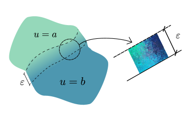
Here is a small parameter, is a double well potential vanishing at two points, say and (the simplified prototype being ), and represents the phase of the fluid, where correspond to one stable phase and to the other one. According to this gradient theory for first order phase transitions, observed stable configurations minimize the energy under a mass constraint , for some fixed .
The gradient term present in the energy (1.1) provides a selection criterion among minimizers of . If neglected then every field such that in and satisfying the mass constraint is a minimizer of . The singular perturbation provides a selection criterion and it competes with the potential term in that it penalizes inhomogeneities of and acts as a regularization for the problem. In particular, the parameter is related to the thickness of the transition layer between the two phases. It was conjectured by Gurtin (see [27]) that for the minimizer of the energy will approximate a piecewise constant function, , taking values in the zero set of the potential , and minimizing the surface area of the interface separating the two phases. Here denotes the -dimensional Hausdorff measure and is the set of jump points of .
Gurtin’s conjecture has been proved by Modica in [32] (see also the work of Sternberg [36]) using -convergence techniques introduced by De Giorgi and Franzoni in [17]. In particular, it has been showed that
where the constant plays the role of the surface energy density per unit area required to make a transition from one stable phase to the other, and it is given by
Several variants of the Van der Waals-Cahn-Hilliard gradient theory for phase transitions have been studied analytically. Here we recall the extension to the case of non-interacting immiscible fluids, with a vector-valued density . In [25] Fonseca and Tartar treated the case of two stable phases (i.e., the potential has two zeros), while the general case of several stable phases has been solved by Baldo in [6]. In [6] and [25] it has been proved that the limit of a sequence , where is a minimizer of , is a minimal partition of the container , where each set satisfies a volume constraint and corresponds to a stable phase, i.e., a zero of .
Other generalizations of (1.1) include the work of Bouchitté [8], who studied the case of a fluid where its two stable phases change from point to point, in order to treat the situation where the temperature of the fluid is not constant inside the container, but given a priori. From the mathematical point of view, this corresponds to considering the energy (1.1) with a potential of the form vanishing on the graphs of two non constant functions .
Fonseca and Popovici in [24] dealt with the vectorial case of the energy (1.1) where the term is substituted with a more general expression of the form , while the full coupled singular perturbed problem in the vectorial case, with the energy density of the form , has been studied by Barroso and Fonseca in [7].
The case in which Dirichlet boundary conditions are considered was addressed by Owen, Rubinsten and Sternberg in [35], while in [33] Modica studied the case of a boundary contact energy.
We refer to the works [36] of Sternberg and [1] of Ambrosio for the case where the zeros of the potential are generic compact sets.
Finally, in [28] Kohn and Sternberg studied the convergence of local minimizers for singular perturbation problems.
This paper is part of an ongoing project aimed at studying the interaction between phase transitions and homogenization, namely when small scale heterogeneities are present in the fluids. In particular, we treat the case of a mixture of non-interacting immiscible fluids with two minimizing phases in isothermal conditions. To be precise, for we consider the energy
| (1.2) |
where is a double well potential that is -periodic in the first variable and with two zeros (see Section 1.1 for more precise details on the hypotheses on ). The small scale heterogeneities are modeled by the fast oscillations in the first variable of the potential .
Since , in order to understand the behavior of minimizing sequences as we need to consider the rescaled energy . In the main result of this paper (see Theorem 1.6) we identify the variational limit (in the sense of -convergence) of the rescaled energies as . In particular, we will prove that the limiting energy is given by an anisotropic surface functional. We refer to Section 1.1 for the precise statement of the result. Since the scaling of the energy coincides with the scaling of the fine oscillations in the potential, we expect to observe, in the limit, an interaction between the phase transition and the homogenization process.
The transition layer between the two phases has a thickness of size , which is the same scale of the micro-structures that form within this layer due to the potential term. The main challenge of this work will be to handle the situation in which the orientation of the interface is not aligned with the directions of periodicity of the potential . This misalignment will give rise to the anisotropy in the limiting energy (see Figure 2). In particular, the cell problem for the limiting energy density (see Definition 1.3) cannot be reduced to a one dimensional optimal profile problem, as in the case of the energy (1.1) (see Figure 1). This phenomenon is well known in models for solid-solid phase transitions, when higher derivatives are considered in the energy (see, for instance, [13]).
The case where different scalings are present, namely when the small heterogeneities are at a scale with
, will be treated in a forthcoming paper.
Moreover, the case in which the wells of the potential depend on the spatial variable , modeling non-isothermal condition, is currently under investigation.
In the literature we can find other problems treating simultaneously phase transitions and homogenization. In [5] (see also [4]) Ansini, Braides and Chiadò Piat considered the family of functionals
and identified the -limit in all three regimes
| (1.3) |
using abstract -convergence techniques to prove the general form of the limiting functional, and more explicit arguments to derive the explicit expression in the three regimes (actually, in the first case they need to assume as ).
Moreover, we mention the articles [19] and [20] by Dirr, Lucia and Novaga regarding a model for phase transition with an additional bulk term modeling the interaction of the fluid with a periodic mean zero external field. In [19] they considered, for , the family of functionals
for some , while in [20] they treated the case
where . Notice that is a particular case of when and has vanishing normal derivative on . An explicit expression of the -limit is provided in both cases.
The work [11] by Braides and Zeppieri is similar in spirit to the ongoing project of ours where we consider the case of the wells of depending on the space variable . Indeed, in [11] the authors studied the asymptotic behavior of the family of functionals
for and the potential defined, for , as
with . For the fact that the zeros of oscillate at a scale of leads to the formation of microscopic oscillations, whose effect is studied by identifying the zeroth, the first and the second order -limit expansions (with the appropriate rescaling) in the three regimes (1.3).
In the context of the gradient theory for solid-solid phase transition, we mention the work [26] by Francfort and Müller, where the asymptotic behavior of the energy
for is studied under some growth conditions on the potential .
Finally, in [30] the authors studied the gradient flow of the energy (1.2) in the case where the parameter in front of the term is kept fixed and only the parameter in is allowed to vary.
1.1. Statement of the main result
In the following denotes the unit cube centered at the origin with faces orthogonal to the coordinate axes, . Consider a double well potential satisfying the following properties:
-
(H0)
is -periodic for all ,
-
(H1)
is a Carathéodory function, i.e.,
-
(i)
for all the function is measurable,
-
(ii)
for a.e. the function is continuous,
-
(i)
-
(H2)
there exist such that if and only if , for a.e. ,
-
(H3)
there exists a continuous function such that for a.e. and if and only if .
-
(H4)
there exist and such that for a.e. and all .
Remark 1.1.
The choice is connected to the exponent we used in the term of the energy (1.2). If that term is substituted with , in (H4) we would need to take .
Hypotheses (H1), (H2) (H3) and (H4) conform with the prototypical potential
where are measurable pairwise disjoint sets with , and are continuous functions with quadratic growth at infinity and such that if and only if , modeling the case of a heterogeneous mixture composed of different compositions. Here in (H3) may be taken as .
Let be an open bounded set with Lipschitz boundary. For consider the energy defined as
| (1.4) |
where denotes the Euclidean norm of the matrix (matrices with rows and columns).
We introduce some definitions. For , with the unit sphere of , we denote by the family of cubes centered at the origin with two faces orthogonal to and with unit length sides.
Definition 1.2.
Let and define the function as
| (1.5) |
Fix a function with , where is the unit ball in . For , set and
| (1.6) |
When it is clear from the context, we will abbreviate as .
Definition 1.3.
We define the function as
where
and
Just as before, if there is no possibility of confusion, we will write as .

Remark 1.4.
For every , is well defined and finite (see Lemma 4.1) and its definition does not depend on the choice of the mollifier (see Lemma 4.3). Moreover, the function is upper semi-continuous on (see Proposition 4.4).
Using [9], it is possible to prove that the infimum in the definition of may be taken with respect to one fixed cube . Namely, given and it holds
Remark 1.5.
In the context of homogenization when dealing with nonconvex potentials it is natural to consider, in the cell problem for the limiting density function , the infimum over all possible cubes . For instance, this was observed by Müller in [34], where the asymptotic behavior as of the family of functionals
defined for , is studied. The limiting energy is of the form
with
In the case where is convex, the infimum over is not needed (see [31]).
Consider the functional defined by
| (1.7) |
where and denotes the measure theoretic external unit normal to the reduced boundary of at (see Definition 2.6).
We now state the main result of this paper that ensures compactness of energy bounded sequences and identifies the asymptotic behavior of the energies .
Theorem 1.6.
Let be a sequence such that as . Assume that (H0), (H1), (H2), (H3) and (H4) hold.
-
(i)
If is such that
then, up to a subsequence (not relabeled), in , where ,
-
(ii)
As , it holds .
Moreover, the function is continuous.
Remark 1.7.
The limiting functional is an anisotropic perimeter functional, whose limiting energy density is defined via a cell problem describing the intricate interaction between homogenization and phases transition. It is interesting to notice that in phase transitions models of the form
one would expect the limiting model to be isotropic if is. Instead, in our case, the anisotropy originates from the mismatch between the square related to the periodicity of , and a square having two faces orthogonal to the normal to the interface.
Once Theorem 1.6 is established, using well known arguments to deal with the mass constraint (see [32]) and the result by Kohn and Sternberg ([28]) for approximating isolated local minimizers, we also obtain the following.
Corollary 1.8.
Let and consider, for , the functionals given by
Under the assumptions of Theorem 1.6 it holds that , where is given by
In particular, every cluster point of a sequence of -minimizers for is a minimizer for , and, moreover, every isolated local minimizer of can be obtained as the limit of , where is a local minimizer of .
The proof of the Theorem 1.6 will be divided in several parts. We would like to briefly comment on the main ideas we will use.
After recalling some preliminary concepts in Section 2 and establishing auxiliary technical results in Section 3, we will prove the compactness result of Theorem 1.6 (i) (see Proposition 5.1) by reducing our functional to the standard Cahn-Hilliard energy (1.1).
In Proposition 6.1 we will obtain the liminf inequality by using the blow-up method introduced by Fonseca and Müller in [22] (see also [23]). Although this strategy can nowadays be considered standard, for clarity and completeness we include the argument.
The limsup inequality is presented in Proposition 7.1 and requires new geometric ideas. This is due to the fact that the periodicity of in the first variable is an essential ingredient to build a recovery sequence. It turns out (see Proposition 3.5) that there exists a dense set such that, for every there exists and for which for a.e. , all and all , and such that is an orthonormal basis of . Using this fact, in the first step of the proof of Proposition 7.1 we obtain a recovery sequence for the special class of functions for which the normals to the interface , where , belong to . We decided to construct a recovery sequence only locally, in order to avoid the technical problem of gluing together optimal profiles for different normal directions to the transition layer. For this reason, we first prove that the localized version of the -limit is a Radon measure absolutely continuous with respect to , and then we show that its density, identified using cubes whose faces are orthogonal to elements of , is bounded above by . Finally, in the second step we conclude using a density argument that will invoke Reshetnyak’s upper semi-continuity theorem (see Theorem 2.9) and the upper semi-continuity of (see Proposition 4.4).
2. Preliminaries
In this section we collect basic notions needed in the paper.
2.1. Finite nonnegative Radon measures
The family of finite nonnegative Radon measures on a topological space will be denoted by .
Definition 2.1.
Let be a -compact metric space. We say that a sequence weakly- converges to a finite nonnegative Radon measure if
as , for all , where is the completion in the norm of the space of continuous functions with compact support on . In this case we write .
The following compactness result for Radon measures is well known (see [21, Proposition 1.202]).
Theorem 2.2.
Let be a -compact metric space and let be such that . Then the exist a subsequence (not relabeled) and such that .
2.2. Sets of finite perimeter
We recall the definition and some well known facts about sets of finite perimeter (we refer the reader to [3] for more details).
Definition 2.3.
Let with and let be an open set. We say that has finite perimeter in if
Remark 2.4.
is a set of finite perimeter in if and only if , i.e., the distributional derivative is a finite vector valued Radon measure in , with
for all , and .
Remark 2.5.
Let be an open set, let , and let . Then is a function of bounded variation in , and we write , if the set has finite perimeter in .
Definition 2.6.
Let be a set of finite perimeter in the open set . We define , the reduced boundary of , as the set of points for which the limit
exists and is such that . The vector is called the measure theoretic exterior normal to at .
We now recall the structure theorem for sets of finite perimeter due to De Giorgi (see [3, Theorem 3.59] for a proof of the following theorem).
Theorem 2.7.
Let be a set of finite perimeter in the open set . Then
-
(i)
for all the set converges locally in as to the halfspace orthogonal to and not containing ,
-
(ii)
,
-
(iii)
the reduced boundary is -rectifiable, i.e., there exist Lipschitz functions , , such that
where each is a compact set.
Remark 2.8.
Finally, we state a result due to Reshetnyak in the form we will need in this paper (for a statement and proof of the general case see, for instance, [3, Theorem 2.38]).
Theorem 2.9.
Let be a sequence of sets of finite perimeter in the open set such that and , where is a set of finite perimeter in . Let be an upper semi-continuous bounded function. Then
2.3. -convergence
Definition 2.10.
Let be a metric space. We say that -converges to , and we write , if the following hold:
-
(i)
for every and every we have
-
(ii)
for every there exists (so called a recovery sequence) with such that
In the proof of the limsup inequality we will need to show that a certain set function is actually (the restriction to the family of open sets of) a finite Radon measure. The classical way to prove this is by using the De Giorgi-Letta coincidence criterion (see [18]), namely to show that the set function is inner regular as well as super and sub additive. In this paper we will use a simplified coincidence criterion due to Dal Maso, Fonseca and Leoni (see [15, Corollary 5.2]). Given an open set, we denote by the family of all open subsets of .
Lemma 2.11.
Let be an increasing set function such that:
-
(i)
for all with it holds
-
(ii)
, for all with ,
-
(iii)
there exists a measure such that
for all , where denotes the family of Borel sets of .
Then is the restriction to of a measure defined on .
3. Preliminary technical results
The first result relies on De Giorgi’s slicing method (see [16]), and it allows to adjust the boundary conditions of a given sequence of functions without increasing the energy, by carefully selecting where to make the transition from the given function to one with the right boundary conditions. Although the argument is nowadays considered to be standard, we include it here for the convenience of the reader.
For , we localize the functional by setting
where and . Also, for , we define
Lemma 3.1.
Let be a cube with and let . Let with be cubes, let with as , and let , with , satisfy
-
(i)
in ,
-
(ii)
in ,
-
(iii)
.
Let with . Then there exists a sequence , with in , where is defined as in (1.6), for some with as , such that
Moreover, in as , where is as in (H4).
Proof.
Assume, without loss of generality, that
| (3.1) |
and that, as , for a.e. .
Step 1. We claim that
| (3.2) |
Indeed, using (H4), we get
| (3.3) |
for . From (3.1) we have as for a.e. , and thus
where we used Fatou’s lemma and (3.3).
Step 2. Here we abbreviate as . Set and . Using Step 1, since we get . For every divide into equidistant layers of width , for . It holds
| (3.4) |
For every let , with , be such that
| (3.5) |
where
Further, consider cut-off functions with
| (3.6) |
such that
| (3.7) |
| (3.8) |
Set
It holds that . Let be such that . Then in . We claim that
| (3.9) |
Indeed
| (3.10) |
To estimate the first term in (3) we notice that
| (3.11) |
Consider the term . Using (H4) together with (3.6) we have that
| (3.12) |
where in the last step we used (3.5) and the fact that . Since for a cube with side length we have
and the cubes are all contained in the bounded cube , we can find such that for all and we get
| (3.13) |
Step 1 (see (3.2)) yields
| (3.14) |
Moreover, by (3.4) we obtain
| (3.15) |
| (3.16) |
and, since
| (3.17) |
| (3.18) |
From (3), (3.13), (3.14), (3.15), (3.16) and (3.18) we get
| (3.19) |
We now estimate the term . Using (3.17), we obtain
and so
| (3.20) |
Similarly, it holds that
| (3.21) |
Using (3), (3.11), (3.19), (3.20) and (3.21) we obtain (3.9).
Applying a diagonalizing argument, it is possible to find an increasing sequence such that
and . Thus, the sequence , with satisfies the claim of the lemma. ∎
Remark 3.2.
The proof of the limsup inequality, Proposition 7.1, uses periodicity properties of the potential energy . In particular, we will show that is periodic in the first variable not only with respect to the canonical set of orthogonal direction, but also with respect to a dense set of orthogonal directions. In the sequel we will use the notation and will denote the standard orthonormal basis for . We first recall the following extension theorem for isometries (for a proof see, for instance, [29, Theorem 10.2]).
Theorem 3.3.
(Witt’s Extension Theorem) Let be a finite dimensional vector space over a field with characteristic different from , and let be a symmetric bilinear form on with for all . Let be subspaces of and let be an isometry, that is, for all . Then can be extended to an isometry from to .
Lemma 3.4.
Let . Then there exist a rotation and such that and for all .
Proof.
Let be fixed. Consider the spaces
as subspaces of over the field , with being the standard Euclidean inner product. Then, the linear map defined by is an isometry. Apply Theorem 3.3 to extend as a linear isometry . In particular, . Up to redefining the sign of so that , we can assume to be a rotation. Let be such that for all . Finally, define to be the unique continuous extension of to all of , which is well defined as isometries are uniformly continuous. ∎
Proposition 3.5.
Let . Then there exist and such that is an orthonormal basis of , and for a.e. it holds for all and .
Proof.
Let be a rotation and let be given by Lemma 3.4 relative to . Set for . We have that for all . Fix and write , for some . For , using the periodicity of with respect to the canonical directions, for a.e. we have that
∎
In the following, given a linear map , we will denote by the Euclidean norm of , i.e., . For the sake of notation, we will also define the set of rational rotations as the rotations such that for .
Lemma 3.6.
Let , , and let be a rotation with . Then there exists a rotation such that and .
Proof.
Step 1 We claim that is dense in for every .
We proceed by induction on . When , consists of the identity, so the claim is trivial. Let be fixed and let and be arbitrary. By density of , we can find a sequence with such that as . By Lemma 3.4 we can find such that . Since is a compact set, we can extract a convergent subsequence (not relabeled) of such that , with .
Thus, the rotation fixes and may be identified with a rotation , i.e., writing , it follows that . By the induction hypotheses, we can find such that
Define by
Let be so large that
We claim that our desired rotation is . Indeed,
Step 2 Let with be given. If , there is nothing else to prove, so we proceed with .
By Lemma 3.4 we can find a rotation such that . Since is a rotation with , as in Step 1 we can identify with a rotation . Also by Step 1, is dense in , so we can find such that . As before, identifying with a rotation that fixes , we set . We have that and
∎
Definition 3.7.
Let . We say that a set is a -polyhedral set if is a Lipschitz manifold contained in the union of finitely many affine hyperplanes each of which is orthogonal to an element of .
A variant of well known approximation results of sets of finite perimeter by polyhedral sets yields the following (see [3, Theorem 3.42]).
Lemma 3.8.
Let be a dense set. If is a set with finite perimeter in , then there exists a sequence of -polyhedral sets such that
Proof.
Using [3, Theorem 3.42] it is possible to find a family of polyhedral sets such that
For every , let be the hyperplanes whose union contains the boundary of . Let be such that . Then it is possible to find rotations such that and, denoting by the set enclosed by the hyperplanes , we get
∎
4. Properties of the function
The aim of this section is to study properties of the function introduced in Definition 1.3 that we will need in the proof of Proposition 7.1 in order to prove the limsup inequality.
Lemma 4.1.
Let . Then is well defined and is finite.
Proof.
Let . For let and be such that
| (4.1) |
where, for simplicity of notation, we write for . Let be an orthonormal basis of normal to the faces of such that . We define an oriented rectangular prism centered at 0 via
Let . We claim that for all with , we have
| (4.2) |
where the quantity does not depend on and is such that
Note that if this holds then
and this ensures the existence of the limit in the definition of . Therefore, the remainder of Step 1 is dedicated to proving (4.2).
The idea is to construct a competitor for the infimum problem defining by taking copies of centered on in each of which we define to be (a translation of) .
In order to compare the energy of to the energy of , we need the copies of the cube to be integer translations of the original. Moreover, we also have to ensure that the boundary conditions render admissible for the infimum problem defining . For this reason, we need the centers of the translated copies of to be close to (recall that the mollifiers and only depend on the direction ).
Set
and notice that
| (4.3) |
We can tile with disjoint prisms so that
for each . In each cube we can find since dist in , and we have
Consider, for and cut-off functions be such that
| (4.4) |
for some . Define by
Notice that since , if we have
Thus and, if then , so is admissible for the infimum in the definition of . In particular,
| (4.5) |
where
and we set
We now bound each of terms separately. We start with . Since , the periodicity of together with (4.1) yield
| (4.6) |
In order to estimate , notice that, since for every the function is constant outside of an interval of size , we have that for every it holds
| (4.7) |
Thus, using (4.4) and (4) we obtain
| (4.8) |
where in the last step we used the inequality
| (4.9) |
for , that is valid here when .
We can finally estimate as
| (4.10) |
Remark 4.2.
Next we show that the definition of does not depend on the choice of the mollifier we choose to impose the boundary conditions.
Lemma 4.3.
For every the definition of does not depend on the choice of the mollifier .
Proof.
Fix and let be such that as . Let be two mollifiers and let us denote by and the functions defined as in Definition 1.3 using and , respectively, to impose the boundary conditions for the admissible class of functions. Let and with on be such that
| (4.13) |
For every , consider the cubes and a function with such that in , on . For every define as
We now prove a regularity property for the function .
Proposition 4.4.
The function is upper semi-continuous.
Proof.
Step 1. Fix and let be such that as . We first prove that, for fixed , the function is continuous. We claim that . Fix . Let and be such that
| (4.15) |
Without loss of generality, by density, we can assume that . For every , let be a rotation such that and as , where is the identity map. Moreover, thanks to Lemma 4.3, we can assume the mollifier and the rotations to be such that for all and . Notice that it is possible to satisfy this condition because for all . Define as . By (4.15) we have
| (4.16) |
where
We claim that as . Since is arbitrary in (4), this would confirm the claim.
Fix and let , where and are given by (H4). Let be a compact set such that and for every . Notice that for all . Using the Scorza-Dragoni theorem (see [21, Theorem 6.35]) and the Tietze extension theorem (see [21, Theorem A.5]), we can find a compact set with and continuous map such that for all and for every . We claim that
| (4.17) |
and that
| (4.18) |
Indeed
A similar argument yields (4.18). Since is bounded
| (4.19) |
as . Thus, from (4.17), (4.18) and (4.19) we obtain
The claim follows from the arbitrariness of .
In an analogous way it is possible to show that , and thus we conclude that the function is continuous.
Step 2. Fix , , and let be such that
| (4.20) |
Let be a sequence converging to . By Step 1 we have that
| (4.21) |
Then, for , using (4.2) and (4.20) we get, for ,
Taking the limit as we obtain
Letting , by (4.21)
Finally, taking and then , using (4.12), we conclude that
for every , and thus we obtain upper-semicontinuity. ∎
The following technical results, that will be fundamental in the proof of the limsup inequality (see Proposition 7.1), aim at providing two different ways to obtain, for , the value .
Lemma 4.5.
Let . Then
| (4.22) |
where
and is the family of cubes with unit length side centered at the origin with two faces orthogonal to and the other faces orthogonal to elements of .
Proof.
Fix . From the definition of it follows that
| (4.23) |
Let with as . By Lemma 4.1, let and with be such that
| (4.24) |
For every fixed , an argument similar to the one used in Step 1 of the proof of Proposition 4.4 together with Lemma 3.6 ensure that it is possible to find rotations with and for all such that
| (4.25) |
where . Thus
| (4.26) |
where the last step follows from (4.24), while in the second to last step we used (4.25). By (4.23) and (4) and the arbitrariness of the sequence , we conclude (4.22). ∎
Lemma 4.6.
For and define
where
Then there exists such that as . In particular, if it is possible to take .
Proof.
First of all notice that, in view of Remark 4.2, is well defined. By definition, we have for all . Thus, it suffices to prove that it is possible to find a sequence such that , where as . Let be an increasing sequence with as such that
It is then possible to find (or, using Lemma 4.5, in case ) such that for all it holds
| (4.27) |
An argument similar to the one used in Lemma 4.1 to establish (4.2) shows that for every , , , and , it holds
| (4.28) |
where is independent of and of (see (4.12)), and is such that
In particular, for all , it is possible to choose such that
| (4.29) |
Thus, we get
| (4.30) |
From (4.27) and (4.30), sending , we get
Using (4.29) we conclude that
∎
5. Compactness
Proposition 5.1.
Let be a sequence with , where . Then there exists such that, up to a subsequence (not relabeled), in .
Proof.
Let be the continuous function given by (H3). Let be such that for , where and are as in (H4), and . Take a function such that in and in . Define the function by
for . Notice that if and only if . Since for a.e. , we get
and, in turn, we have that . We now proceed as in [25] to obtain a subsequence of and such that in . ∎
6. Liminf inequality
This section is devoted to the proof of the liminf inequality.
Proposition 6.1.
Given a sequence with , let be such that in . Then
Proof.
Let with in . Without loss of generality, and possibly up to a subsequence, we can assume that
| (6.1) |
By Proposition 5.1, we get . Set . Consider, for every , the finite nonnegative Radon measure
From (6.1) we have that . Thus, up to a subsequence (not relabeled), , for some finite nonnegative Radon measure in . In particular,
| (6.2) |
We claim that for -a.e. it holds
| (6.3) |
where .
The liminf inequality follows from (6.2) and (6.3).
The rest of the proof is devoted at showing the validity of (6.3).
Step 1. For -a.e. we have
| (6.4) |
Fix satisfying (6.4) and a cube , with . Let be a sequence with as , such that , where for all . Then it holds
| (6.5) |
We have
| (6.6) |
where in the last step, for the sake of simplicity, we set , we wrote , with and , and we used the periodicity of to simplify, for , ,
Consider the functions , for . We claim that
| (6.7) |
where is defined as in (1.5). Set and its complement in . We get
where , is its complement in and . The last step follows from (i) of Theorem 2.7.
Step 2. Using a diagonal argument, and (6.7), it is possible to find an increasing sequence such that, setting
the following hold:
-
(i)
;
-
(ii)
;
-
(iii)
in for all ;
-
(iv)
we have
From (6.5), (6) and (iv) we get
Let be the largest cube contained in centered at zero and having the same principal axes of . Since as , for large and the integrand is nonnegative, we have that
| (6.8) |
Step 3. Finally we modify close to in order to render it an admissible function for the infimum problem defining as in Definition 1.3. Using Lemma 3.1 we find a sequence such that
| (6.9) |
and with on , where is defined as in (1.6). Hence, by (6.8) and (6.9)
since , where , and this concludes the proof. ∎
7. Limsup inequality
In this section we construct a recovery sequence.
Proposition 7.1.
Let . Given a sequence with as , there exist with in as such that
| (7.1) |
Proof.
Notice that it is enough to prove the following: given any sequence with as , it is possible to extract a subsequence for which there exists with in as such that
Since is separable, we conclude using the Urysohn property of the -limit (see [14, Proposition 8.3]).
Case 1. Assume that the set is a -polyhedral set (see Definition 3.7). We need to localize the -limit of our sequence of functionals. For with , and we set
Let be the family of all open cubes in with faces parallel to the axes, centered at points and with rational edgelength. Denote by the countable subfamily of whose elements are and all finite unions of elements of , i.e.,
Let . We will select a suitable subsequence in the following manner. We enumerate the elements of by . First considering , by a diagonalization argument we can find a subsequence and functions such that
and
Now, considering , we can extract a further subsequence and find functions such that
and
Continuing along the in this fashion and employing a further diagonalization argument, we can assert the existence of a subsequence of with the following property: for every , there exists a sequence such that
and
| (7.2) |
We claim that
-
(C1)
the set function given by
is a positive finite Radon measure absolutely continuous with respect to ,
-
(C2)
for -a.e. , it holds
(7.3)
This allows us to conclude. Indeed, we have that
Step 1. We first prove claim (C1).
We use the coincidence criterion in Lemma 2.11 to show that is the restriction of a positive finite measure to .
We will first prove (i) in Lemma 2.11. Let be such that . For , let and be two elements of such that , , and
| (7.4) |

Let be a symmetric mollifier, and define
| (7.7) |
From Remark 3.2 we can assume that on and on . Using a similar argument to the one found in Lemma 3.1 applied to the sets , and with boundary data , it is possible to find functions with (here we are using the notation of the proof of Lemma 3.1) such that, if we define the function as
we have that and
| (7.8) |
Notice that in as . Moreover, we get
| (7.9) |
where in the last step we used (7.5), (7.6) and (7.8). We see that
| (7.10) |
where in the last step we used (7.4). Using (7), (7) and the fact that and , we get
Letting , we obtain (i).
We proceed to proving (ii) in Lemma 2.11. Let be such that . Fixing , we can find such that and
Then, since the restriction of to and converges to in these sets,
and
by definition, we have
Sending , we conclude
To prove the opposite inequality, as in the proof of (i), we select , with and
| (7.11) |
Again we may select and such that in , in and
| (7.12) |
| (7.13) |
As in the proof of (i) of Lemma 2.11, we may assume without loss of generality that on , on , and we can find functions so that, defining
we have and
| (7.14) |
where , again using the notation of Lemma 3.1. Observing that in , we get
where in the last step we used (7.12), (7.13), and (7.14). Noticing that
and by (7.11) we have
and, letting , we conclude (ii).
We prove (iii) in Lemma 2.11. Let . Recalling (7.7), we know that is constant outside a tubular neighborhood of width around and that . Thus
| (7.15) |
This shows, by the coincidence criterion Lemma 2.11, that is a Radon measure.
Since is a finite Radon measure in and (7.15) holds for every ,
we conclude that is a finite Radon measure in absolutely continuous with respect to , which was the claim (C1).
Step 2. We now prove (C2). Let be on a face of (since the set is polyhedral) and write . Using Proposition 3.5 it is possible to find a rotation and such that, setting , we get and
for a.e. , every that is orthogonal to one face of , every and . By Remark 2.8 it follows that for -almost every ,
| (7.16) |
where . In view of Lemma 4.6, it is possible to find with as , and such that
| (7.17) |
where is defined as and is defined as in Lemma 4.6. Without loss of generality, by density, we can assume . Since the choice of mollifier is arbitrary by Lemma 4.3, we will assume here that and thus
For let and . Moreover, set .
For , extend the function to the whole by periodicity, and define
| (7.18) |
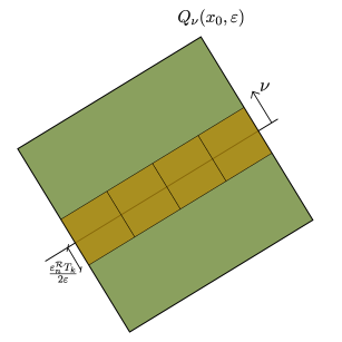
The idea behind the definition of the function is the following (see Figure 5): for every fixed and we are tiling the face of orthogonal to with -rescaled copies of the optimal profile . The fact that is a -polyhedral set and that ensure that it is possible to use the periodicity of to estimate the energy in each cube of edge length . The presence of the factor in (7.18) localizes the function around the point and accommodates the blow-up method we are using to prove the limsup inequality and, because of periodicity, will play no essential role in the fundamental estimate (7.25).
Let and be such that , and let
Note that for every we have
| (7.19) |
Define the functions by
We claim that there is such that for every and any
| (7.20) |
Since is on a face of , we can find such that in . Changing variables,
Since the functions are uniformly bounded with respect to , we prove our claim by noticing that as .
Thus, using the definition of and (7.20), we get
| (7.21) |
We want to rewrite the right-hand side of (7.21) in terms of the functions . To do so, changing variables, we write
where in the second to last step we used the periodicity of .
We claim that
| (7.22) |
Indeed, using Fubini’s Theorem and a change of variables, we have
Fix . By (7.19), for each , let be such that for all . In particular, we have . Set . For every , the functions defined by
are periodic. The Riemann-Lebesgue Lemma yields
| (7.23) |
and
| (7.24) |
for every open and bounded set . Thus we get
Sending we obtain (7.22).
Finally, we claim that
| (7.25) |
Recalling the definition of the functions (see (7.18)) and using Fubini’s Theorem we can write
Thus, using (7) and (7.24) (that are independent of ), we obtain
From (7.21), (7.22) and (7.25) we get
| (7.26) |
In order to conclude, we use Lemma 4.6 to find a sequence such that as . Using (7) we obtain for every
and, letting we have
Using the Urysohn property, we conclude that if the set is -polyhedral, then there exists a sequence with in such that
Case 2. We now consider the general case of a function . Using Lemma 3.8 it is possible to find a sequence of functions with the following properties: the set is a -polyhedral set and, setting , we have
From the result of Case 1, for every it is possible to find a sequence with as , such that
Choose an increasing sequence such that, setting ,
| (7.27) |
Recalling that the function is upper semi-continuous on (see Proposition 4.4), from Theorem 2.9 and (7.27) we get
This concludes the proof of the limsup inequality. ∎
8. Continuity of
To prove that the function is continuous, notice that Theorem 1.6 implies, in particular, that the functional is lower semi-continuous with respect to the convergence. It then follows from [3, Theorem 5.11] that the function , when extended -homogeneously to the whole , is convex. Since for every (see Lemma 4.1), we also deduce that is continuous.
For the convenience of the reader, we recall here the argument used in [3, Theorem 5.11] to prove convexity. Take such that . We claim that . Using the -homogeneity of , this is equivalent to convexity. To prove the claim, let , where is such that and . Let be the the two dimensional space generated by and , consider the unit two dimensional square and a triangle with outer normals and , and such that
are the lengths of the side of orthogonal to , and respectively. Let be the unit cube and . Let be a rotation such that . Let and be such that . Then there exists such that . For , let
where the ’s are such that the elements in the second union are pairwise disjoint and . It can be shown that , so that by lower semi-continuity of we obtain
This proves the claim.
Acknowledgement
We would like to thank the Center for Nonlinear Analysis at Carnegie Mellon University for its support during the preparation of the manuscript. Riccardo Cristoferi, Irene Fonseca and Adrian Hagerty were supported by the National Science Foundation under Grant No. DMS-1411646.
References
- [1] L. Ambrosio, Metric space valued functions of bounded variation, Ann. Scuola Norm. Sup. Pisa Cl. Sci. (4), 17 (1990), pp. 439–478.
- [2] L. Ambrosio and G. Dal Maso, On the relaxation in of quasi-convex integrals, J. Funct. Anal., 109 (1992), pp. 76–97.
- [3] L. Ambrosio, N. Fusco, and D. Pallara, Functions of bounded variation and free discontinuity problems, Oxford Mathematical Monographs, The Clarendon Press, Oxford University Press, New York, 2000.
- [4] N. Ansini, A. Braides, and V. Chiadò Piat, Interactions between homogenization and phase-transition processes, Tr. Mat. Inst. Steklova, 236 (2002), pp. 386–398.
- [5] N. Ansini, A. Braides, and V. Chiadò Piat, Gradient theory of phase transitions in composite media, Proc. Roy. Soc. Edinburgh Sect. A, 133 (2003), pp. 265–296.
- [6] S. Baldo, Minimal interface criterion for phase transitions in mixtures of Cahn-Hilliard fluids, Ann. Inst. H. Poincaré Anal. Non Linéaire, 7 (1990), pp. 67–90.
- [7] A. C. Barroso and I. Fonseca, Anisotropic singular perturbations–the vectorial case, Proc. Roy. Soc. Edinburgh Sect. A, 124 (1994), pp. 527–571.
- [8] G. Bouchitté, Singular perturbations of variational problems arising from a two-phase transition model, Appl. Math. Optim., 21 (1990), pp. 289–314.
- [9] G. Bouchitté, I. Fonseca, and L. Mascarenhas, A global method for relaxation, Arch. Ration. Mech. Anal., 145 (1998), pp. 51–98.
- [10] A. Braides, -convergence for beginners, vol. 22 of Oxford Lecture Series in Mathematics and its Applications, Oxford University Press, Oxford, 2002.
- [11] A. Braides and C. I. Zeppieri, Multiscale analysis of a prototypical model for the interaction between microstructure and surface energy, Interfaces Free Bound., 11 (2009), pp. 61–118.
- [12] J. W. Cahn and J. E. Hilliard, Free energy of a nonuniform system. i. interfacial free energy, J. Chem. Ph.m, 28 (1958), pp. 258–267.
- [13] S. Conti, I. Fonseca, and G. Leoni, A -convergence result for the two-gradient theory of phase transitions, Comm. Pure Appl. Math., 55 (2002), pp. 857–936.
- [14] G. Dal Maso, An Introduction to -Convergence, Springer, 1993.
- [15] G. Dal Maso, I. Fonseca, and G. Leoni, Nonlocal character of the reduced theory of thin films with higher order perturbations, Adv. Calc. Var., 3 (2010), pp. 287–319.
- [16] E. De Giorgi, Sulla convergenza di alcune successioni d’integrali del tipo dell’area, Rend. Mat. (6), 8 (1975), pp. 277–294. Collection of articles dedicated to Mauro Picone on the occasion of his ninetieth birthday.
- [17] E. De Giorgi and T. Franzoni, Su un tipo di convergenza variazionale, Atti Accad. Naz. Lincei Rend. Cl. Sci. Fis. Mat. Natur. (8), 58 (1975), pp. 842–850.
- [18] E. De Giorgi and G. Letta, Une notion générale de convergence faible pour des fonctions croissantes d’ensemble, Ann. Scuola Norm. Sup. Pisa Cl. Sci. (4), 4 (1977), pp. 61–99.
- [19] N. Dirr, M. Lucia, and M. Novaga, -convergence of the Allen-Cahn energy with an oscillating forcing term, Interfaces Free Bound., 8 (2006), pp. 47–78.
- [20] N. Dirr, M. Lucia, and M. Novaga, Gradient theory of phase transitions with a rapidly oscillating forcing term, Asymptot. Anal., 60 (2008), pp. 29–59.
- [21] I. Fonseca and G. Leoni, Modern methods in the calculus of variations: spaces, Springer Monographs in Mathematics, Springer, New York, 2007.
- [22] I. Fonseca and S. Müller, Quasi-convex integrands and lower semicontinuity in , SIAM J. Math. Anal., 23 (1992), pp. 1081–1098.
- [23] , Relaxation of quasiconvex functionals in for integrands , Arch. Ration. Mech. Anal., 123 (1993), pp. 1–49.
- [24] I. Fonseca and C. Popovici, Coupled singular perturbations for phase transitions, Asymptot. Anal., 44 (2005), pp. 299–325.
- [25] I. Fonseca and L. Tartar, The gradient theory of phase transitions for systems with two potential wells, Proc. Roy. Soc. Edinburgh Sect. A, 111 (1989), pp. 89–102.
- [26] G. A. Francfort and S. Müller, Combined effects of homogenization and singular perturbations in elasticity, J. Reine Angew. Math., 454 (1994), pp. 1–35.
- [27] M. E. Gurtin, Some results and conjectures in the gradient theory of phase transitions, in Metastability and incompletely posed problems (Minneapolis, Minn., 1985), vol. 3 of IMA Vol. Math. Appl., Springer, New York, 1987, pp. 135–146.
- [28] R. V. Kohn and P. Sternberg, Local minimisers and singular perturbations, Proc. Roy. Soc. Edinburgh Sect. A, 111 (1989), pp. 69–84.
- [29] S. Lang, Algebra, vol. 211 of Graduate Texts in Mathematics, Springer-Verlag, New York, third ed., 2002.
- [30] M. Liero and S. Reichelt, Homogenization of Cahn-Hilliard-type equations via evolutionary -convergence, NoDEA Nonlinear Differential Equations Appl., 25 (2018), pp. Art. 6, 31.
- [31] P. Marcellini, Periodic solutions and homogenization of nonlinear variational problems, Ann. Mat. Pura Appl. (4), 117 (1978), pp. 139–152.
- [32] L. Modica, The gradient theory of phase transitions and the minimal interface criterion, Arch. Ration. Mech. Anal., 98 (1987), pp. 123–142.
- [33] , Gradient theory of phase transitions with boundary contact energy, Ann. Inst. H. Poincaré Anal. Non Linéaire, 4 (1987), pp. 487–512.
- [34] S. Müller, Homogenization of nonconvex integral functionals and cellular elastic materials, Arch. Ration. Mech. Anal., 99 (1987), pp. 189–212.
- [35] N. C. Owen, J. Rubinstein, and P. Sternberg, Minimizers and gradient flows for singularly perturbed bi-stable potentials with a Dirichlet condition, Proc. Roy. Soc. London Ser. A, 429 (1990), pp. 505–532.
- [36] P. Sternberg, The effect of a singular perturbation on nonconvex variational problems, Arch. Ration. Mech. Anal., 101 (1988), pp. 209–260.
- [37] J. D. Van der Waals, The thermodynamics theory of capillarity under the hypothesis of a continuous variation of density, Verhaendel Kronik. Akad. Weten. Amsterdam, 1 (1893), pp. 386–398.