Semi-discrete unbalanced optimal transport and quantization

Abstract

In this paper we study the class of optimal entropy-transport problems introduced by Liero, Mielke and Savaré in Inventiones Mathematicae 211 in 2018. This class of unbalanced transport metrics allows for transport between measures of different total mass, unlike classical optimal transport where both measures must have the same total mass. In particular, we develop the theory for the important subclass of semi-discrete unbalanced transport problems, where one of the measures is diffuse (absolutely continuous with respect to the Lebesgue measure) and the other is discrete (a sum of Dirac masses). We characterize the optimal solutions and show they can be written in terms of generalized Laguerre diagrams. We use this to develop an efficient method for solving the semi-discrete unbalanced transport problem numerically. As an application we study the unbalanced quantization problem, where one looks for the best approximation of a diffuse measure by a discrete measure with respect to an unbalanced transport metric. We prove a type of crystallization result in two dimensions – optimality of the triangular lattice – and compute the asymptotic quantization error as the number of Dirac masses tends to infinity.

1 Introduction

In this paper we study semi-discrete unbalanced optimal transport problems: What is the optimal way of transporting a diffuse measure to a discrete measure (hence the name semi-discrete), where the two measures may have different total mass (hence the name unbalanced)? As an application we study the unbalanced quantization problem: What is the best approximation of a diffuse measure by a discrete measure with respect to an unbalanced transport metric?

1.1 What is unbalanced optimal transport?

Classical optimal transport theory asks for the most efficient way to rearrange mass between two given probability distributions. Its origin goes back to 1781 and the French engineer Gaspard Monge, who was interested in the question of how to transport and reshape a pile of earth to form an embankment at minimal effort. It took over 200 years to develop a complete mathematical understanding of this problem, even to answer the question of whether there exists an optimal way of redistributing mass. Since the mathematical breakthroughs of the 1980s and 1990s, the field of optimal transport theory has thrived and found applications in crowd and traffic dynamics, economics, geometry, image and signal processing, machine learning and data science, PDEs, and statistics. Depending on the context, mass may represent the distribution of particles (people or cars), supply and demand, population densities, etc. For thorough introductions see, e.g., [20, 42, 45, 50].

In classical optimal transport theory it is not necessary that the initial and target measures are both probability measures, but they must have the same total mass. In applications this is not always natural. Changes in mass may occur due to creation or annihilation of particles or a mismatch between supply and demand. Therefore so-called unbalanced transport problems, accounting for such differences, have recently received increased attention [14, 19, 30, 33]. Brief overviews and discussions of various formulations can be found, for instance, in [13, 46]. In this article we study the class of unbalanced transport problems called optimal entropy-transport problems from [33]; see Definition 2.4. In particular, we develop this theory for the special case of semi-discrete transport.

1.2 What is semi-discrete transport?

Semi-discrete optimal transport theory is about the best way to transport a diffuse measure, $\mu\in L^{1}(\Omega)$, $\Omega\subset\mathbb{R}^{d}$, to a discrete measure, $\nu=\sum_{i=1}^{M}m_{i}\delta_{x_{i}}$. These type of problems arise naturally, for instance, in economics in computing the distance between a population with density $\mu$ and a resource with distribution $\nu=\sum_{i=1}^{M}m_{i}\delta_{x_{i}}$, where $x_{i}\in\Omega$ represent the locations of the resource and $m_{i}>0$ represent the size or capacity of the resource. The classical semi-discrete optimal transport problem, where $\mu$ and $\nu$ are probability measures, has a nice geometric characterization. For example, for $p\in[1,\infty)$, the Wasserstein-$p$ metric $W_{p}$ is defined by

$$W_{p}(\mu,\nu)=\min\left\{\sum_{i=1}^{M}\int_{T^{-1}(x_{i})}|x-x_{i}|^{p}\mu(x)\,\textnormal{d}x\,\right.\left|\,T:\Omega\to\{x_{i}\}_{i=1}^{M},\,\int_{T^{-1}(x_{i})}\mu(x)\,\textnormal{d}x=m_{i}\right\}^{1/p}$$

where $\sum_{i=1}^{M}m_{i}=\int_{\Omega}\mu(x)\,\textnormal{d}x=1$. This is an optimal partitioning (or assignment) problem, where the domain $\Omega$ is partitioned into the regions $T^{-1}(x_{i})$ of mass $m_{i}$, $i\in\{1,\ldots,M\}$, and each point $x\in T^{-1}(x_{i})$ is assigned to point $x_{i}$. For example, in two dimensions, $\Omega$ could represent a city, $\mu$ the population density of children, $x_{i}$ and $m_{i}$ the location and size of schools, $T^{-1}(x_{i})$ the catchment areas of the schools, and $W_{p}(\mu,\nu)$ the cost of transporting the children to their assigned schools. If $p=2$, it turns out that the optimal partition $\{T^{-1}(x_{i})\}_{i=1}^{M}$ is a Laguerre diagram or power diagram, which is a type of weighted Voronoi diagram: There exist weights $w_{1},\ldots,w_{M}\in\mathbb{R}$ such that

$$\overline{T^{-1}(x_{i})}=\{x\in\Omega\,|\,|x-x_{i}|^{2}-w_{i}\leq|x-x_{j}|^{2}-w_{j}\,\forall\,j\in\{1,\ldots,M\}\}.$$

The transport cells $T^{-1}(x_{i})$ are the intersection of convex polytopes (polygons if $d=2$, polyhedra if $d=3$) with $\Omega$. The weights $w_{1},\ldots,w_{M}\in\mathbb{R}$ can be found by solving an unconstrained concave maximization problem. If $p=1$, the optimal partition $\{T^{-1}(x_{i})\}_{i=1}^{M}$ in an Apollonius diagram. See, e.g., [3, Sec. 6.4], [20, Chap. 5], [28], [42, Chap. 5], and Section 2.3 below, where we summarize the main results from classical semi-discrete optimal transport theory.

In Section 3 we extend these results to unbalanced transport, where $\mu$ and $\nu$ no longer need to have the same total mass, and the Wasserstein-$p$ metric is replaced by the unbalanced transport metric $W$ from Definition 2.4. We prove that, also in the unbalanced case, the optimal partition is a type of generalized Laguerre diagram and it can be found by solving a concave maximization problem for a set of weights $w_{1},\ldots,w_{M}$; see Theorems 3.1 and 3.2. This problem is natural from a modelling perspective, for example to describe a mismatch between the demand of a population $\mu$ and the supply of a resource $\nu$, and to model the prioritization of high-density regions at the expense of areas with a low population density.

For unbalanced transport, there is no one, definitive transport cost. As as first application of our theory of semi-discrete unbalanced transport, in Examples 3.13 and 3.14, we use it to compare different unbalanced transport models. As a second application, in Section 4, we apply it to the quantization problem.

1.3 What is quantization?

Quantization of measures refers to the problem of finding the best approximation of a diffuse measure by a discrete measure [24], [27, Sec. 33]. For example, the classical quantization problem with respect to the Wasserstein-$p$ metric, $p\in[1,\infty)$, is the following: Given $\mu\in L^{1}(\Omega)$, $\Omega\subset\mathbb{R}^{d}$, $\int_{\Omega}\mu(x)\,\textnormal{d}x=1$, find a discrete probability measure $\nu=\sum_{i=1}^{M}m_{i}\delta_{x_{i}}$ that gives the best approximation of $\mu$ in the Wasserstein-$p$ metric,

$$Q^{M}_{p}(\mu)=\min\left\{W_{p}^{p}(\mu,\nu)\,\Bigg{|}\,\nu=\sum_{i=1}^{M}m_{i}\delta_{x_{i}},\;x_{1},\ldots,x_{M}\in\Omega,\;m_{i}>0,\;\sum_{i=1}^{M}m_{i}=1\right\}.$$ (1.1)

We call $Q^{M}_{p}$ the quantization error. Problems of this form arise in a wide range of applications including economic planning and optimal location problems [6, 7, 11], finance [41], numerical integration [15, Sec. 2.2], [41, Sec. 2.3], energy-driven pattern formation [10, 31], and approximation of initial data for particle (meshfree) methods for PDEs. If $\mu$ is a discrete measure, with support of cardinality $N\gg M$, then applications include image and signal compression [16, 23] and data clustering ($k$-means clustering) [36, 47]. If $\nu$ is a one dimensional measure (supported on a set of Hausdorff dimension $1$), then the quantization problem is known as the irrigation problem [35, 39]. An alternative approach to quantization using gradient flows is given in [12].

It can be shown that the quantization problem (1.1) can be rewritten as an optimization problem in terms of the particle locations $\{x_{i}\}_{i=1}^{M}$ and their Voronoi tessellation:

$$Q^{M}_{p}(\mu)=\min\left\{J(x_{1},\ldots,x_{M})\,|\,x_{1},\ldots,x_{M}\in\Omega\right\}$$ (1.2)

where

$$J(x_{1},\ldots,x_{M})=\sum_{i=1}^{M}\int_{V_{i}(x_{1},\ldots,x_{M})}|x-x_{i}|^{p}\mu(x)\,\textnormal{d}x$$

and where $\{V_{i}\}_{i=1}^{M}$ is the Voronoi diagram generated by $\{x_{i}\}_{i=1}^{M}$,

$$V_{i}=V_{i}(x_{1},\ldots,x_{M})=\left\{x\in\Omega\,\middle|\,|x-x_{i}|\leq|x-x_{j}|\textnormal{ for all }j\in\{1,\ldots,M\}\right\}.$$

If $(x_{1},\ldots,x_{M})$ is a global minimizer of $J$, then $\sum_{i=1}^{M}\left(\int_{V_{i}}\mu\,\textnormal{d}x\right)\delta_{x_{i}}$ is an optimal quantizer of $\mu$ with respect to the Wasserstein-$p$ metric. See for instance [10, Sec. 4.1], [29, Sec. 7] and Theorem 4.1. In the vector quantization (electrical engineering) literature $J$ is known as the distortion of the quantizer [23].

The quantization problem with respect to the Wasserstein-2 metric is particularly well studied. In this case it can be shown that critical points of $J$ are generators of centroidal Voronoi tessellations (CVTs) of $M$ points [15]; this means that $\nabla J(x_{1},\ldots,x_{M})=0$ if and only if $x_{i}$ is the centre of mass of its own Voronoi cell $V_{i}$ for all $i$,

$$x_{i}=\frac{\displaystyle\int_{V_{i}(x_{1},\ldots,x_{M})}x\mu(x)\,\textnormal{d}x}{\displaystyle\int_{V_{i}(x_{1},\ldots,x_{M})}\mu(x)\,\textnormal{d}x},\quad i\in\{1,\ldots,M\}.$$ (1.3)

In general there does not exist a unique CVT of $M$ points, as illustrated in Fig. 1, and $J$ is non-convex with many local minimisers for large $M$. Equation (1.3) is a nonlinear system of equations for $x_{1},\ldots,x_{M}$. A simple and popular method for computing CVTs is Lloyd’s algorithm [15, 18, 34, 44], which is a fixed point method for solving the Euler-Lagrange equations (1.3).

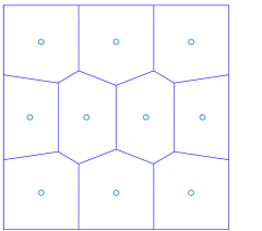
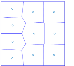
Figure 1: Two (approximate) centroidal Voronoi tessellations (CVTs) of 10 points for the uniform density $\mu=1$ on a unit square. The polygons are the centroidal Voronoi cells $V_{i}$ and the circles are the generators $x_{i}$. The CVTs were computed using Lloyd’s algorithm. The CVT on the left has a lower energy $J$ than the CVT on the right. The corresponding quantizer $\nu=\sum_{i=1}^{10}m_{i}\delta_{x_{i}}$ of $\mu$ is reconstructed from the CVT by taking $m_{i}$ as the areas of the centroidal Voronoi cells and $x_{i}$ as their generators.

In Sections 4.1 and 4.2 we extend these results to unbalanced quantization, where the Wasserstein-$p$ metric in (1.1) is replaced by the unbalanced transport metric $W$ (defined in equation (2.6)) and where $\mu$ and $\nu$ need not have the same total mass. In Theorem 4.1 we prove an expression of the form $\eqref{eq:ClassicalQuantizationTessellation}$, which states that the unbalanced quantization problem can be reduced to an optimization problem for the locations $x_{1},\ldots,x_{M}$ of the Dirac masses. This optimization problem is again formulated in terms of the Voronoi diagram generated by $x_{1},\ldots,x_{M}$. In Section 4.2 we solve the unbalanced quantization problem numerically, which includes extending Lloyd’s algorithm to the unbalanced case.

We conclude the paper in Section 4.3 by studying the asymptotic unbalanced quantization problem: What is the optimal configuration of the particles $x_{1},\ldots,x_{M}$ as $M\to\infty$? How does the quantization error scale in $M$? Consider for example the classical quantization problem (1.1) with $p=2$, $|\Omega|=1$, $\mu=1$ and $M$ fixed. From above, we know that an optimal quantizer $\nu$ corresponds to an optimal CVT of $M$ points, where optimal means that the CVT has lowest energy $J$ amongst all CVTs of $M$ points. Gersho [22] conjectured that, as $M\to\infty$, the Voronoi cells of the optimal CVT asymptotically have the same shape, i.e., asymptotically they are translations and rescalings of a single polytope. In two dimensions ($d=2$) various versions of Gersho’s Conjecture have been proved independently by several authors who, roughly speaking, showed that the optimal CVT of $M$ points tends to a regular hexagonal tiling as $M\to\infty$ [6, 25, 38, 40, 48, 49]. In other words, the optimal locations $x_{1},\ldots,x_{M}$ tend to a regular triangular lattice. This crystallization result can be stated more precisely as follows: If $\Omega$ is a convex polygon with at most 6 sides, then

$$J(x_{1},\ldots,x_{M})\geq\frac{5\sqrt{3}}{54}\frac{1}{M}$$ (1.4)

where the right-hand side is the energy of a regular triangular lattice of $M$ points such that the Voronoi cells $V_{i}$ are regular hexagons of area $1/M$. In general this lower bound is not attained for finite $M$ (unless $\Omega$ is a regular hexagon and $M=1$), but it is attained in limit $M\to\infty$ (for any reasonable domain $\Omega$),

$$\lim_{M\to\infty}M\cdot Q_{2}^{M}(1)=\lim_{M\to\infty}M\cdot\min_{x_{i}\in\Omega}J(x_{1},\ldots,x_{M})=\frac{5\sqrt{3}}{54}.$$ (1.5)

See the references above or [8, Thm. 5]. We generalise (1.4) and (1.5) to the unbalanced quantization problem in Theorem 4.6 and Theorem 4.14. Roughly speaking, we show that again the triangular lattice is optimal in the limit $M\to\infty$. For general $\mu\in L^{1}(\Omega)$, the particles locally form a triangular lattice with density determined by a nonlocal function of $\mu$.

While our quantization results are limited to two dimensions, this is also largely true for the classical quantization problem. In three dimensions it is not known whether Gersho’s Conjecture holds, although there is some numerical evidence for the case $p=2$ that optimal CVTs of $M$ points tend as $M\to\infty$ to the Voronoi diagram of the body-centered cubic (BCC) lattice, where the Voronoi cells are congruent to truncated octahedra [17]. Also, for $p=2$, it has been proved that, amongst lattices, the BCC lattice is optimal [4]. For general $p$ and general dimension $d$ the scaling of the quantization error is known even if the optimal quantizer is not; Zador’s Theorem [51],[27, Cor. 33.3] states that

$$Q^{M}_{p}(1)\sim\frac{c(p,d)|\Omega|^{\frac{p+d}{d}}}{M^{\frac{p}{d}}}$$

as $M\to\infty$. See also [29, Thm. 1.2],[26]. It remains however an open problem to compute the constant $c(p,d)$.

1.4 Outline and Contribution

Section 2 collects relevant results from classical, unbalanced, and semi-discrete transport, which will be generalized in Section 3 to the case of semi-discrete unbalanced transport. Finally, Section 4 considers the unbalanced quantization problem.

In more detail, the contributions of this article are the following.

• Section 3.1: We extend semi-discrete transport theory to the unbalanced case, including different primal and dual convex formulations, optimality conditions, and most importantly a simple, geometric tessellation formulation (Theorem 3.1) which turns out to be only slightly more complicated than the corresponding formulation for classical semi-discrete transport.

• Section 3.2: We develop numerical algorithms for solving the semi-discrete unbalanced transport problem and numerically illustrate novel phenomena of unbalanced transport (Example 3.13). In particular, we show qualitative differences between different unbalanced transport models and examine the effect of changing the length scale, which typically is intrinsic to unbalanced transport models.

• Sections 4.1 and 4.2: We extend the theory of optimal transport-based quantization of measures to unbalanced transport, deriving in particular an equivalent Voronoi tessellation problem (Theorem 4.1), which turns out to be just as simple as the known corresponding formulation in classical transport. The interesting fact here is that the simple geometric Voronoi tessellation structure survives when passing from balanced to unbalanced transport. We also illustrate unbalanced quantization numerically, extending the standard algorithms to the unbalanced case.

• Section 4.3: In two spatial dimensions, where crystallization results from discrete geometry are available, we derive the optimal asymptotic quantization cost and the optimal asymptotic point density for quantizing a given measure $\mu$ using unbalanced transport (Theorem 4.14). The interesting, novel effect in this unbalanced setting is that the optimal point density depends nonlocally on the global mass distribution in such a way that whole regions with positive measure may be completely neglected in favour of regions with higher mass.

1.5 Setting and Notation

Throughout this article we work in a domain $\Omega=\overline{U}$ for $U\subset\mathbb{R}^{d}$ open and bounded. (In principle, results could be extended to more general metric spaces such as Riemannian manifolds.) The Euclidean distance on $\mathbb{R}^{d}$ is denoted $d(\cdot,\cdot)$, and we will write $\pi_{i}:\Omega\times\Omega\to\Omega$, for the projections $\pi_{i}(x_{1},x_{2})=x_{i}$, $i=1,2$. The ($d$-dimensional) Lebesgue measure of a measurable set $A\subset\mathbb{R}^{d}$ will be indicated by $\mathcal{L}(A)$ or $|A|$ for short, its diameter by $\text{diam}(A)$.

By ${\mathcal{M}_{+}}(\Omega)$ we denote the set of nonnegative Radon measures on $\Omega$, and ${\mathcal{P}}(\Omega)\subset{\mathcal{M}_{+}}(\Omega)$ is the subset of probability measures. The notation $\mu\ll\nu$ for two measures $\mu,\nu\in{\mathcal{M}_{+}}(\Omega)$ indicates absolute continuity of $\mu$ with respect to $\nu$, and the corresponding Radon–Nikodym derivative is written as $\tfrac{\textnormal{d}\mu}{\textnormal{d}\nu}$. The restriction of $\mu\in{\mathcal{M}_{+}}(\Omega)$ to a measurable set $A\subset\mathbb{R}^{d}$ is denoted $\mu{\mbox{\LARGE$\llcorner$}}A$, and its support is denoted $\operatorname{spt}\mu$. For a Dirac measure at a point $x\in\mathbb{R}^{d}$ we write $\delta_{x}$. The pushforward of a measure $\mu$ under a measurable map $T$ is denoted ${T}_{\#}\mu$.

The spaces of Lebesgue integrable functions on $U$ or of $\mu$-integrable functions with $\mu\in{\mathcal{M}_{+}}(\Omega)$ are denoted $L^{1}(U)$ and $L^{1}(\mu)$, respectively. Continuous functions on $\Omega$ are denoted by $\mathcal{C}(\Omega)$.

2 Background

The purpose of this section is a short introduction to classical, unbalanced, and semi-discrete transport.

2.1 Optimal transport

Here we briefly recall the basic setting of optimal transport. For a thorough introduction we refer, for instance, to [45, 50]. For $\mu$, $\nu\in{\mathcal{P}}(\Omega)$ the set

$$\Gamma(\mu,\nu)=\{\gamma\in{\mathcal{P}}(\Omega\times\Omega)\,|\,{\pi_{1}}_{\#}\gamma=\mu,\,{\pi_{2}}_{\#}\gamma=\nu\}$$ (2.1)

is called the couplings or transport plans between $\mu$ and $\nu$. A measure $\gamma\in\Gamma(\mu,\nu)$ can be interpreted as a rearrangement of the mass of $\mu$ into $\nu$ where $\gamma(x,y)$ intuitively describes how much mass is taken from $x$ to $y$. The total cost associated to a coupling $\gamma$ is given by

$$\int_{\Omega\times\Omega}c(x,y)\,\textnormal{d}\gamma(x,y)$$ (2.2)

where $c:\Omega\times\Omega\to[0,\infty]$ and $c(x,y)$ specifies the cost of moving one unit of mass from $x$ to $y$. The optimal transport problem asks for finding a $\gamma$ that minimizes (2.2) among all couplings $\Gamma(\mu,\nu)$,

$$W_{\textnormal{OT}}(\mu,\nu)=\inf\left\{\int_{\Omega\times\Omega}c\,\textnormal{d}\gamma\,\middle|\,\gamma\in\Gamma(\mu,\nu)\right\}\,.$$ (2.3)

Under suitable regularity assumptions on $c$, existence of minimizers follows from standard compactness and lower semi-continuity arguments.

Theorem 2.1 ([50, Thm. 4.1]).

If $c:\Omega\times\Omega\to[0,\infty]$ is lower semi-continuous, then minimizers of (2.3) exist. The minimal value may be $+\infty$.

2.2 Unbalanced transport

The optimal transport problem (2.3) only allows the comparison of measures $\mu$, $\nu$ with equal mass. Otherwise, the feasible set $\Gamma(\mu,\nu)$ is empty. Therefore, so-called unbalanced transport problems have been studied, where mass may be created or annihilated during transport and thus measures of different total mass can be compared in a meaningful way. See Section 1 for context and references.

Throughout this article we consider unbalanced optimal entropy-transport problems as studied in [33]. The basic idea is to replace the hard marginal constraints ${\pi_{1}}_{\#}\gamma=\mu$, ${\pi_{2}}_{\#}\gamma=\nu$ in (2.1) with soft constraints where the deviation between the marginals of $\gamma$ and the measures $\mu$ and $\nu$ is penalized by a marginal discrepancy function. This allows more flexibility for feasible $\gamma$. We focus on a subset of the family of marginal discrepancies considered in [33].

Definition 2.2 (Marginal discrepancy).

Let $F:[0,\infty)\to[0,\infty]$ be proper, convex, and lower semi-continuous with $\lim_{s\to\infty}\tfrac{F(s)}{s}=\infty$. For a given measure $\mu\in{\mathcal{M}_{+}}(\Omega)$, the function $F$ induces a marginal discrepancy $\mathcal{F}(\cdot|\mu):{\mathcal{M}_{+}}(\Omega)\to[0,\infty]$ via

$$\mathcal{F}(\rho|\mu)=\begin{cases}\int_{\Omega}F\big{(}\tfrac{\textnormal{d}\rho}{\textnormal{d}\mu}\big{)}\,\textnormal{d}\mu&\textnormal{if }\rho\ll\mu,\\ +\infty&\textnormal{otherwise.}\end{cases}$$ (2.4)

Note that the integrand is only defined $\mu$-almost everywhere. $\mathcal{F}$ is (sequentially) weakly-$\ast$ lower semi-continuous [1, Thm. 2.34].

We extend the domain of definition of $F$ to $\mathbb{R}$ by setting $F(s)=\infty$ for $s<0$. The Fenchel–Legendre conjugate of $F$ is then the convex function $F^{\ast}:\mathbb{R}\to(-\infty,+\infty]$ defined by

$$F^{\ast}(z)=\sup_{s\in\mathbb{R}}\left(z\cdot s-F(s)\right)=\sup_{s\geq 0}\left(z\cdot s-F(s)\right).$$

Example 2.3 (Kullback–Leibler divergence).

The Kullback–Leibler divergence is an example of Definition 2.2 for the choice $F_{\textnormal{KL}}:[0,\infty)\to[0,\infty)$,

$$F_{\textnormal{KL}}(s)=\begin{cases}s\log s-s+1&\textnormal{if }s>0,\\ 1&\textnormal{if }s=0.\end{cases}$$

The Fenchel–Legendre conjugate is given by $F_{\textnormal{KL}}^{\ast}(z)=e^{z}-1$.

Definition 2.4 (Unbalanced optimal transport problem).

Let $F$ be as in Definition 2.2 and let $\mathcal{F}$ be the induced marginal discrepancy. Let $\mu$, $\nu\in{\mathcal{M}_{+}}(\Omega)$ and $c:\Omega\times\Omega\to[0,\infty]$ be lower semi-continuous. The corresponding unbalanced transport cost $\mathcal{E}:{\mathcal{M}_{+}}(\Omega\times\Omega)\to[0,\infty]$ is given by

$$\mathcal{E}(\gamma)=\int_{\Omega\times\Omega}c\,\textnormal{d}\gamma+\mathcal{F}({\pi_{1}}_{\#}\gamma|\mu)+\mathcal{F}({\pi_{2}}_{\#}\gamma|\nu)$$ (2.5)

and induces the optimization problem

$$W(\mu,\nu)=\inf\left\{\mathcal{E}(\gamma)\,\middle|\,\gamma\in{\mathcal{M}_{+}}(\Omega\times\Omega)\right\}.$$ (2.6)

Theorem 2.5 ([33, Thm. 3.3]).

Minimizers of (2.6) exist. The minimal value may be $+\infty$.

Remark 2.6.

Observe that $\mathcal{F}(\rho|\mu)=\infty$ whenever $\rho\not\ll\mu$ and $\mathcal{F}(\rho|\nu)=\infty$ whenever $\rho\not\ll\nu$. This guarantees that ${\pi_{1}}_{\#}\gamma\ll\mu$ and ${\pi_{2}}_{\#}\gamma\ll\nu$ for all feasible $\gamma$, where feasible means that $\mathcal{E}(\gamma)<\infty$. Thus, when $\mu\ll\mathcal{L}$ and $\nu$ is discrete, as in the semi-discrete setting (which will be discussed in the following section), then the first and second marginal of any feasible $\gamma$ will share these properties.

In this article we focus on cost functions $c$ that can be written as increasing functions of the distance between $x$ and $y$.

Definition 2.7 (Radial cost).

A cost function $c:\Omega\times\Omega\to[0,\infty]$ is called radial if it can be written as $c(x,y)=\ell(d(x,y))$ for a strictly increasing function $\ell:[0,\infty)\to[0,\infty]$, continuous on its domain with $\ell(0)=0$.

The following examples shall be used throughout for illustration. They all feature a radial transport cost $c$ in the sense of Definition 2.7.

Example 2.8 (Unbalanced transport models).

1. Standard Wasserstein-2 distance (W2). Classical balanced optimal transport can be recovered as a special case of Definition 2.4 by choosing $\mathcal{F}(\rho|\mu)=0$ if $\rho=\mu$ and $\infty$ otherwise. This corresponds to

   $$F(s)=\iota_{\{1\}}(s) =\begin{cases}0&\textnormal{if }s=1,\\ \infty&\textnormal{otherwise,}\end{cases} F^{\ast}(z) =z\,.$$

   Then $\mathcal{E}(\gamma)<\infty$ only if $\gamma\in\Gamma(\mu,\nu)$, and therefore (2.6) reduces to (2.3). In particular, the Wasserstein-2 setting is obtained for $c(x,y)=d(x,y)^{2}$, and the Wasserstein-2 distance is defined by $W_{2}(\mu,\nu)=\sqrt{W(\mu,\nu)}$.

2. Gaussian Hellinger–Kantorovich distance (GHK). This distance is introduced in [33, Thm. 7.25] using

   $$F(s) =F_{\textnormal{KL}}(s)=\begin{cases}s\log s-s+1&\textnormal{if }s>0,\\ 1&\textnormal{if }s=0,\end{cases} F^{\ast}(z) =e^{z}-1\,, c(x,y) =d(x,y)^{2}\,.$$

3. Wasserstein–Fisher–Rao or Hellinger–Kantorovich distance (WFR). This important instance of unbalanced transport was introduced in different formulations in [30, 14, 33] whose mutual relations are described in [13]. In Definition 2.4 one chooses

   $$F(s)=F_{\textnormal{KL}}(s)\,,\quad F^{\ast}(z)=e^{z}-1\,,$$

   $$c(x,y)=c_{\textnormal{WFR}}(x,y)=\begin{cases}-2\log\big{[}\cos\big{(}d(x,y)\big{)}\big{]}&\textnormal{if }d(x,y)<\tfrac{\pi}{2},\\ \infty&\textnormal{otherwise,}\end{cases}\quad$$

   and the Wasserstein–Fisher–Rao distance is defined by $\textnormal{WFR}(\mu,\nu)=\sqrt{W(\mu,\nu)}$. The distance WFR is actually a geodesic distance on the space of non-negative measures over a metric base space. From $c_{\textnormal{WFR}}(x,y)=\infty$ for $d(x,y)\geq\tfrac{\pi}{2}$, we learn that mass is never transported further than $\tfrac{\pi}{2}$ in this setting.

4. Quadratic regularization (QR). The Kullback–Leibler discrepancy $F_{\textnormal{KL}}$ used in both previous examples has an infinite slope at $0$, which in Definition 2.4 leads to a strong incentive to achieve ${\pi_{1}}_{\#}\gamma\gg\mu$ and ${\pi_{2}}_{\#}\gamma\gg\nu$. The following mere quadratic discrepancy does not have this property,

   $$F(s) =(s-1)^{2}\,, F^{\ast}(z) =\begin{cases}\tfrac{z^{2}}{4}+z&\textnormal{if }z\geq-2,\\ -1&\textnormal{otherwise,}\end{cases} c(x,y) =d(x,y)^{2}\,.$$

Unsurprisingly, the structure of the function $F$ has a great influence on the behaviour of the unbalanced optimization problem (2.6). Often it is helpful to analyze corresponding dual problems where the conjugate function $F^{\ast}$ appears. We gather some properties of $F^{\ast}$, implied by the assumptions on $F$ in Definition 2.2 and on some additional assumptions that we will occasionally make in this article.

Lemma 2.9 (Properties of $F^{\ast}$).

Let $F$ satisfy the assumptions given in Definition 2.2. Then

1. $F^{\ast}(z)>-\infty$ for $z\in\mathbb{R}$;

2. $F^{\ast}$ is increasing;

3. $F^{\ast}(z)\leq 0$ for $z\leq 0$;

4. $F^{\ast}(z)<\infty$ for $z\in(0,\infty)$;

5. $F^{\ast}$ is real-valued and continuous on $\mathbb{R}$;

6. if $F$ is strictly convex on its domain, then $F^{\ast}$ is continuously differentiable on $\mathbb{R}$;

7. if $F(0)<\infty$, then $F^{\ast}(z)\geq-F(0)$ for all $z\in\mathbb{R}$ and

   $$\lim_{z\to-\infty}\min\partial F^{\ast}(z)=\lim_{z\to-\infty}\max\partial F^{\ast}(z)=0.$$

Proof.

(i) Since $F$ is proper, we can find $s\in(0,\infty)$ with $F(s)<\infty$. Then for all $z\in\mathbb{R}$, $F^{\ast}(z)=\sup_{x\geq 0}(z\cdot x-F(x))\geq z\cdot s-F(s)>-\infty$.

(ii) Let $z_{1}\leq z_{2}$. Then $F^{\ast}(z_{2})=\sup_{x\geq 0}(z_{2}\cdot x-F(x))\geq\sup_{x\geq 0}(z_{1}\cdot x-F(x))=F^{\ast}(z_{1})$.

(iii) Let $z\leq 0$. Since $F\geq 0$, then $F^{\ast}(z)=\sup_{x\geq 0}(z\cdot x-F(x))\leq\sup_{x\geq 0}z\cdot x=0$.

(iv) Let $z\in(0,\infty)$. Since $F\geq 0$, $F^{\ast}(z)=\infty$ is only possible if any maximizing sequence $x_{1},x_{2},\ldots$ for $F^{\ast}(z)=\sup_{x\geq 0}(z\cdot x-F(x))$ is unbounded. However, $\lim_{n\to\infty}(z\cdot x_{n}-F(x_{n}))=\lim_{x\to\infty}x\big{(}z-\tfrac{F(x)}{x}\big{)}=-\infty$ since $\lim_{s\to\infty}\tfrac{F(s)}{s}=\infty$. So $F^{\ast}(z)<\infty$.

(v) (i), (iv), and (iii) imply ${\mathrm{dom}}(F^{\ast})=\mathbb{R}$. By convexity, $F^{\ast}$ is therefore continuous.

(vi) This is a special case of a classical result in convex analysis, which can be found, for instance, in [43, Thm. 26.3].

(vii) Let $z\in\mathbb{R}$. Then $F^{\ast}(z)=\sup_{x\geq 0}(z\cdot x-F(x))\geq-F(0)$. Moreover, let $z_{1},z_{2},\ldots$ and $u_{1},u_{2},\ldots$ be sequences with $z_{n}\to-\infty$ as $n\to\infty$ and $u_{n}\in\partial F^{\ast}(z_{n})$. By monotonicity of $F^{\ast}$, (ii), we have $u_{n}\geq 0$. By (iii) and convexity one finds $0\geq F^{\ast}(0)\geq F^{\ast}(z_{n})+u_{n}\cdot(0-z_{n})\geq-F(0)+u_{n}\cdot|z_{n}|$, which implies that $u_{n}\to 0$. ∎

Remark 2.10 (Feasibility for finite $F(0)$).

Note that for $F(0)<\infty$ the trivial transport plan $\gamma=0$ leads to a finite cost in (2.5) so that $W(\mu,\nu)<\infty$ for all $\mu,\nu\in{\mathcal{M}_{+}}(\Omega)$.

2.3 Semi-discrete transport

An important special case of the classical balanced optimal transport problem (2.3) is the case where $\mu$ is absolutely continuous with respect to the Lebesgue measure,

$$\mu\ll\mathcal{L}\,,$$ (2.7a)

and $$\nu$$ is a discrete measure,

$$\nu=\sum_{i=1}^{M}m_{i}\delta_{x_{i}}\,,$$ (2.7b)

with $m_{i}>0$, $x_{i}\in\Omega$, and $x_{i}\neq x_{j}$ for $i\neq j$. See Section 1 for context and references. In this section we review the special structure of problem (2.3) that follows from (2.7). For instance, optimal couplings for (2.3) turn out to have a very particular form: the domain $\Omega$ is partitioned into cells, one cell for each discrete point $x_{i}$, and mass will only be transported from each cell to its corresponding discrete point. The shape of the cells is determined by $\mu$, $\nu$ and the cost function $c$ and can be expressed with the aid of Definition 2.11. Problem (2.3) can be rewritten explicitly as an optimization problem in terms of the cells. This tessellation formulation is given in Theorem 2.13, and its optimality conditions are described in Theorem 2.15.

Definition 2.11 (Generalized Laguerre cells).

Given a transportation cost $c$ and points $x_{1},\ldots,x_{M}\in\Omega$, we define the generalized Laguerre cells corresponding to the weight vector $w\in\mathbb{R}^{M}$ by

$$C_{i}(w)=\left\{x\in\Omega\,\middle|\,c(x,x_{i})<\infty,\,c(x,x_{i})-w_{i}\leq c(x,x_{j})-w_{j}\textnormal{ for all }j\in\{1,\ldots,M\}\right\}$$ (2.8)

for $i\in\{1,\ldots,M\}$. The residual of $\Omega$, the set not covered by any of the cells $C_{i}$, is defined by

$$R=\left\{x\in\Omega\,\middle|\,c(x,x_{i})=\infty\textnormal{ for all }i\in\{1,\ldots,M\}\right\}.$$ (2.9)

Note that $R$ can also be written as $R=\Omega\setminus\big{(}\bigcup_{i=1}^{M}C_{i}(w)\big{)}$, which does not depend on $w\in\mathbb{R}^{M}$. Note also that, if $a=\lambda(1,1,\ldots,1)\in\mathbb{R}^{M}$ is a vector with all components equal, then $C_{i}(w+a)=C_{i}(w)$ for all $i\in\{1,\ldots,M\}$.

Example 2.12 (Generalized Laguerre cells [3]).

1. Voronoi diagrams. If $c$ is radial (see Definition 2.7) and finite, then the collection of generalized Laguerre cells with weight vector $0\in\mathbb{R}^{M}$, $\{C_{i}(0)\}_{i=1}^{M}$, is just the Voronoi diagram generated by the points $x_{1},\ldots,x_{M}$. The residual set $R=\emptyset$.

2. Laguerre diagrams or power diagrams. If $c(x,y)=|x-y|^{2}$, then the collection of generalized Laguerre cells $\{C_{i}(w)\}_{i=1}^{M}$ is known as the Laguerre diagram or power diagram generated by the weighted points $(x_{1},w_{1}),\ldots,(x_{M},w_{M})$. The cells $C_{i}$ are the intersection of convex polytopes with $\Omega$. The residual set $R=\emptyset$.

3. Apollonius diagrams. If $c(x,y)=|x-y|$, then the collection of generalized Laguerre cells $\{C_{i}(w)\}_{i=1}^{M}$ is known as the Apollonius diagram generated by the weighted points $(x_{1},w_{1}),\ldots,(x_{M},w_{M})$. The cells $C_{i}$ are the intersection of star-shaped sets with $\Omega$, and in two dimensions the boundaries between cells are arcs of hyperbolas. Again, $R=\emptyset$.

Theorem 2.13 (Dual tessellation formulation for semi-discrete transport).

Assume that $\mu$ and $\nu$ satisfy (2.7) and $\mu(\Omega)=\nu(\Omega)$. Let the cost function $c$ be radial (see Definition 2.7) and $W_{\textnormal{OT}}(\mu,\nu)<\infty$. Then

$$W_{\textnormal{OT}}(\mu,\nu)=\sup\left\{\sum_{i=1}^{M}\int_{C_{i}(w)}c(x,x_{i})\,\textnormal{d}\mu(x)+\sum_{i=1}^{M}\big{(}m_{i}-\mu(C_{i}(w))\big{)}\cdot w_{i}\,\middle|\,w\in\mathbb{R}^{M}\right\}.$$ (2.10)

Remark 2.14 (Existence of optimal weights).

Maximizers for (2.10) do not always exist, even when $W_{\textnormal{OT}}(\mu,\nu)<\infty$. A simple sufficient condition for existence is that $c$ is bounded from above on $\Omega\times\Omega$. More details can be found, for instance, in [50, Thm. 5.10].

Theorem 2.15 (Optimality conditions).

Under the conditions of Theorem 2.13, a coupling $\gamma\in\Gamma(\mu,\nu)$ and a vector $w\in\mathbb{R}^{M}$ are optimal for $W_{\textnormal{OT}}(\mu,\nu)$ in (2.3) and (2.10) respectively, if and only if

$$\gamma =\sum_{i=1}^{M}\left(\mu{\mbox{\LARGE$\llcorner$}}{C_{i}(w)}\otimes\delta_{x_{i}}\right), \mu(C_{i}(w)) =m_{i}\textnormal{ for }i\in\{1,\ldots,M\}.$$ (2.11)

Proofs of Theorem 2.13 and Theorem 2.15 can be found below and for example in [2] or [28] under various assumptions on $c$. The latter relies on the existence of an optimal Monge map $T:\Omega\to\{x_{i}\}_{i=1}^{M}$ such that $\nu={T}_{\#}\mu$ and $\gamma={(\operatorname{Id}\times T)}_{\#}\mu$ is optimal for $W_{\textnormal{OT}}(\mu,\nu)$ in (2.3) and arguments based on Kantorovich duality (cf. [50, Thm. 5.10]). Existence of a Monge map for radial, finite, strictly convex cost functions follows for instance from [21, Thm. 1.2].

We provide proofs of Theorems 2.13 and 2.15 for two reasons: They serve as preparation for the proof of Theorems 3.1 and 3.2 in the case of semi-discrete unbalanced transport, which generalize Theorems 2.13 and 2.15. In addition, they deal with the technical aspect that our cost function may take the value $+\infty$ at finite distances. For this we rely on the following lemma, which essentially provides the existence of a Monge map in the semi-discrete setting (Corollary 2.17).

Lemma 2.16 (Laguerre cell boundaries).

Let the cost function $c$ be radial in the sense of Definition 2.7 and let $\{x_{i}\}_{i=1}^{M}$ be $M$ distinct points in $\Omega$. The induced generalized Laguerre cells satisfy $|C_{i}(w)\cap C_{j}(w)|=0$ for $i\neq j$.

Proof.

Fix $i\neq j$ and $w\in\mathbb{R}^{M}$ and recall that $c(x,y)=\ell(d(x,y))$. We have

$$C_{i}(w)\cap C_{j}(w)=\bigcup_{n\in\mathbb{N}}A_{n}\quad\text{for }A_{n}=\{x\in\Omega\,|\,c(x,x_{i})-w_{i}=c(x,x_{j})-w_{j},\,c(x,x_{i})\leq n\}\,,$$

and we will show that the $d$-dimensional Hausdorff measure of each $A_{n}$ is zero, ${\mathcal{H}}^{d}(A_{n})=0$, which implies $|A_{n}|=0$ and thus also $|C_{i}(w)\cap C_{j}(w)|=0$. Indeed, as a Borel set, $A_{n}\subset\mathbb{R}^{d}$ is countably ${\mathcal{H}}^{d}$-rectifiable (since it is ${\mathcal{H}}^{d}$-measurable). Thus, abbreviating $f=d(\cdot,x_{i})$, the coarea formula [1, Thm. 2.93] yields

$${\mathcal{H}}^{d}(A_{n})=\int_{A_{n}}1\,\textnormal{d}{\mathcal{H}}^{d}=\int_{\mathbb{R}}{\mathcal{H}}^{d-1}(A_{n}\cap f^{-1}(t))\,\textnormal{d}t=\int_{0}^{\ell^{-1}(n)}{\mathcal{H}}^{d-1}(A_{n}\cap f^{-1}(t))\,\textnormal{d}t\,.$$

Now, for $t\in[0,\ell^{-1}(n)]$,

$$A_{n}\cap f^{-1}(t)=\{x\in\Omega\,|\,d(x,x_{i})=t\text{ and }d(x,x_{j})\in\ell^{-1}(\ell(d(x,x_{i}))+w_{j}-w_{i})\},$$

where $\ell^{-1}(\ell(d(x,x_{i}))+w_{j}-w_{i})$ is either empty or single-valued due to the strict monotonicity of $\ell$. Hence, $A_{n}\cap f^{-1}(t)$ is contained in the intersection of two non-concentric $(d-1)$-dimensional spheres and thus is ${\mathcal{H}}^{d-1}$-negligible. ∎

Proof of Theorem 2.13.

By Kantorovich duality [50, Thm. 5.10] we can write

$$W_{\textnormal{OT}}(\mu,\nu)=\sup\left\{\int_{\Omega}\phi\,\textnormal{d}\mu+\int_{\Omega}\psi\,\textnormal{d}\nu\,\middle|\,\phi\in L^{1}(\mu),\,\psi\in L^{1}(\nu),\right.\\ \left.\vphantom{\int_{\Omega}}\phi(x)+\psi(y)\leq c(x,y)\,\forall\,(x,y)\in\Omega\times\Omega\right\}\,.$$ (2.12)

Since $\nu$ is discrete, $L^{1}(\nu)$ is isomorphic to $\mathbb{R}^{M}$ under the isomorphism $I:L^{1}(\nu)\to\mathbb{R}^{M}$, $\psi\mapsto(\psi(x_{1}),\ldots,\psi(x_{M}))$. The above dual problem thus becomes

$$W_{\textnormal{OT}}(\mu,\nu)=\sup\left\{\int_{\Omega}\phi\,\textnormal{d}\mu+\sum_{i=1}^{M}w_{i}\,m_{i}\,\middle|\,\phi\in L^{1}(\mu),\,w\in\mathbb{R}^{M},\right.\\ \left.\vphantom{\int_{\Omega}}\phi(x)+w_{i}\leq c(x,x_{i})\,\forall\,x\in\Omega,i\in\{1,\ldots,M\}\right\}\,.$$

Next, for fixed $w$, one can explicitly maximize over $\phi$, which corresponds to pointwise maximization subject to the constraint. We denote the maximizer by $\phi_{w}$ to emphasize the dependency on $w$,

$$\phi_{w}(x)=\min\big{\{}c(x,x_{i})-w_{i}\,|\,i=1,\ldots,M\big{\}}\,.$$ (2.13)

Since $W_{\textnormal{OT}}(\mu,\nu)<\infty$ (and $c$ is bounded from below in our setting) one must have $\phi_{w}\in L^{1}(\mu)$ for all $w\in\mathbb{R}^{M}$, and we find

$$W_{\textnormal{OT}}(\mu,\nu)=\sup\{\mathcal{E}_{\textnormal{SD}}(w)\,|\,w\in\mathbb{R}^{M}\}\quad\textnormal{with}\quad\mathcal{E}_{\textnormal{SD}}(w)=\int_{\Omega}\phi_{w}(x)\,\textnormal{d}\mu(x)+\sum_{i=1}^{M}w_{i}\,m_{i}\,.$$ (2.14)

Since $\phi_{w}\in L^{1}(\mu)$ for any $w\in\mathbb{R}^{M}$, the residual set $R$ must be $\mu$-negligible; likewise, the intersection of generalized Laguerre cells is $\mu$-negligible by Lemma 2.16. Consequently,

$$\mathcal{E}_{\textnormal{SD}}(w)=\sum_{i=1}^{M}\int_{C_{i}(w)}\phi_{w}(x)\,\textnormal{d}\mu(x)+\sum_{i=1}^{M}w_{i}\,m_{i}=\sum_{i=1}^{M}\int_{C_{i}(w)}[c(x,x_{i})-w_{i}]\,\textnormal{d}\mu(x)+\sum_{i=1}^{M}w_{i}\,m_{i}\,,$$

which leads to the desired result. ∎

Proof of Theorem 2.15.

The condition $\gamma\in\Gamma(\mu,\nu)$ implies that $\gamma$ can be written as $\gamma=\sum_{i=1}^{M}\gamma_{i}\otimes\delta_{x_{i}}$ where $\gamma_{i}\in{\mathcal{M}_{+}}(\Omega)$, $\gamma_{i}(A):=\gamma(A\times\{x_{i}\})$. Observe that $\sum_{i=1}^{M}\gamma_{i}=\mu$ and $\gamma_{i}(\Omega)=m_{i}$. We obtain

$$W_{\textnormal{OT}}(\mu,\nu)\leq\int_{\Omega\times\Omega}c\,\textnormal{d}\gamma=\sum_{i=1}^{M}\int_{\Omega}c(x,x_{i})\,\textnormal{d}\gamma_{i}(x)\,,$$ (2.15)

where the inequality is an equality if and only if $\gamma$ is optimal. Let $w\in\mathbb{R}^{M}$. From (2.14) with $\phi_{w}$ given by (2.13) we find

$$W_{\textnormal{OT}}(\mu,\nu)\geq\int_{\Omega}\phi_{w}(x)\,\textnormal{d}\mu(x)+\sum_{i=1}^{M}w_{i}\,m_{i}=\sum_{i=1}^{M}\int_{\Omega}\left[\phi_{w}(x)+w_{i}\right]\,\textnormal{d}\gamma_{i}(x)\,,$$ (2.16)

where the inequality is an equality if and only if $w$ is optimal. Subtracting (2.16) from (2.15) yields

$$0\leq\sum_{i=1}^{M}\int_{\Omega}\left[c(x,x_{i})-w_{i}-\phi_{w}(x)\right]\,\textnormal{d}\gamma_{i}(x).$$ (2.17)

with equality if and only if $\gamma$ and $w$ are optimal. By definition of $\phi_{w}$ the integrand in each term of the sum is nonnegative and strictly positive for $x\notin C_{i}(w)$. Therefore (2.17) is an equality if and only if $\gamma_{i}$ is concentrated on $C_{i}(w)$ for all $i\in\{1,\ldots,M\}$. Combining absolute continuity with respect to the Lebesgue measure of $\mu$ and $\gamma_{i}$ and Lemma 2.16 implies that the unique choice is $\gamma_{i}=\mu{\mbox{\LARGE$\llcorner$}}{C_{i}(w)}$. Due to the second marginal constraint this implies $\mu(C_{i}(w))=\gamma_{i}(\Omega)=m_{i}$. ∎

The above results imply the existence of an optimal Monge map for the semi-discrete problem.

Corollary 2.17 (Existence of Monge map).

If a maximizer $w\in\mathbb{R}^{M}$ of (2.10) exists (cf. Remark 2.14), then the optimal coupling $\gamma$ in Theorem 2.13 is induced by a transport map $T:\Omega\to\{x_{i}\}_{i=1}^{M}\subset\Omega$, $\gamma={(\operatorname{Id}\times T)}_{\#}\mu$, defined by $T(x)=x_{i}$ when $x\in C_{i}(w)$. By virtue of Lemma 2.16 and since $\mu\ll\mathcal{L}$, $T$ is well-defined $\mu$-almost everywhere.

Example 2.18 (Optimal tessellations for Wasserstein distances).

Let $\mu$ and $\nu$ satisfy (2.7).

1. Wasserstein-2 distance. Let $c(x,y)=|x-y|^{2}$. If $T$ is an optimal Monge map, then the optimal transport cells $T^{-1}(\{x_{i}\})$ are the Laguerre cells (or power cells) $C_{i}(w)$ with weight vector $w=(\psi(x_{1}),\ldots,\psi(x_{M}))$, where $\psi:\Omega\to\mathbb{R}$ is an optimal Kantorovich potential for the dual transport problem (2.12).

2. Wasserstein-1 distance. Let $c(x,y)=|x-y|$. If $T$ is an optimal Monge map, then the optimal transport cells $T^{-1}(\{x_{i}\})$ are the Apollonius cells $C_{i}(w)$ with weight vector $w=(\psi(x_{1}),\ldots,\psi(x_{M}))$, where $\psi$ is an optimal Kantorovich potential.

3 Semi-discrete unbalanced transport

In this section we consider semi-discrete unbalanced transport. That is, we study (2.6) for the cases where $\mu$ is absolutely continuous with respect to the Lebesgue measure and $\nu$ is discrete, as stated in (2.7), and we do not require that $\mu(\Omega)=\nu(\Omega)$. Semi-discrete unbalanced transport models the situation where there is a mismatch between the capacity of a discrete resource $\nu$ and the demand of a population $\mu$.

3.1 Tessellation formulation

The main results of this Section are Theorems 3.1 and 3.2, which generalize Theorems 2.13 and 2.15 to the unbalanced setting. Furthermore, in Corollary 3.5 we state a ‘primal’ counterpart of Theorem 3.1 which is somewhat pathological in the classical, balanced optimal transport setting, but quite natural in the unbalanced case.

The following result generalizes Theorem 2.13 to unbalanced transport.

Theorem 3.1 (Tessellation formulation for semi-discrete unbalanced transport).

Given $\mu,\nu\in{\mathcal{M}_{+}}(\Omega)$ satisfying (2.7), define $\mathcal{G}:\mathbb{R}^{M}\to(-\infty,\infty]$ by

$$\mathcal{G}(w)=-\sum_{i=1}^{M}\left(\int_{C_{i}(w)}F^{\ast}\big{(}-c(x,x_{i})+w_{i}\big{)}\,\textnormal{d}\mu(x)+F^{\ast}(-w_{i})\cdot m_{i}\right)+F(0)\cdot\mu(R).$$ (3.1a)

Then the unbalanced optimal transport distance can be obtained via

$$W(\mu,\nu)=\sup\left\{\mathcal{G}(w)\,\middle|\,w\in\mathbb{R}^{M}\right\}.$$ (3.1b)

This is a concave maximization problem.

Proof.

In analogy to the Kantorovich duality (2.12) for the classical optimal transport problem (2.3) we make use of a corresponding duality result for the unbalanced transport problem (2.6),

$$W(\mu,\nu)=\sup\left\{-\int_{\Omega}F^{\ast}(-\phi(x))\,\textnormal{d}\mu(x)-\int_{\Omega}F^{\ast}(-\psi(x))\,\textnormal{d}\nu(x)\,\middle|\,\phi,\psi\in\mathcal{C}(\Omega),\right.\\ \left.\vphantom{\int_{\Omega}}\phi(x)+\psi(y)\leq c(x,y)\,\forall\,(x,y)\in\Omega\times\Omega\right\}.$$

This follows from [33, Thm. 4.11 and Cor. 4.12], where the former establishes the duality formula with $\phi$ and $\psi$ ranging over all lower semi-continuous simple functions and the latter allows us to use continuous functions instead, exploiting the fact that $F^{\ast}$ is continuous on $\mathbb{R}$ by Lemma 2.9(v). Analogously to the proof of Theorem 2.13 we now parameterize the function $\psi$ on the set $\{x_{i}\}_{i=1}^{M}$ by a vector $w\in\mathbb{R}^{M}$, $w_{i}=\psi(x_{i})$, and obtain

$$W(\mu,\nu)=\sup\left\{-\int_{\Omega}F^{\ast}(-\phi(x))\,\textnormal{d}\mu(x)-\sum_{i=1}^{M}m_{i}F^{\ast}(-w_{i})\,\middle|\,\phi\in\mathcal{C}(\Omega),w\in\mathbb{R}^{M},\right.\\ \left.\vphantom{\sum_{i=1}^{M}}\phi(x)+w_{i}\leq c(x,x_{i})\,\forall\,x\in\Omega,i\in\{1,\ldots,M\}\right\}.$$ (3.2)

Next, given $w\in\mathbb{R}^{M}$ we would like to optimize for $\phi$ as we did in (2.13). Note though that $\phi_{w}=\infty$ on the residual set $R$, which in unbalanced transport may be nonnegligible despite finite $W(\mu,\nu)$. For this reason we argue by truncation: For given $w\in\mathbb{R}^{M}$ and $n\in\mathbb{N}$, the function $\phi=\phi_{w,n}$ with

$$\phi_{w,n}:\Omega\to\mathbb{R},\quad\phi_{w,n}(x)=\min\{n,\min\{c(x,x_{i})-w_{i}\,|\,i\in\{1,\ldots,M\}\}\}$$

lies in $\mathcal{C}(\Omega)$ and is feasible in (3.2). Moreover, for fixed $w$ the sequence $(\phi_{w,n})_{n\in\mathbb{N}}$ is a maximizing sequence for the maximization over $\phi$, and it converges pointwise monotonically to the function $\phi_{w}$ defined in (2.13). By Lemma 2.9(ii) and (v), $z\mapsto-F^{\ast}(-z)$ is continuous and increasing. Therefore the monotone convergence theorem implies that

$$\lim_{n\to\infty}\int_{\Omega}F^{\ast}(-\phi_{w,n}(x))\,\textnormal{d}\mu(x)=\int_{\Omega}F^{\ast}(-\phi_{w}(x))\,\textnormal{d}\mu(x)\,,$$

where by convention $F^{\ast}(-\infty)=\lim_{z\to-\infty}F^{\ast}(z)=-F(0)$ (see Lemma 2.9). With this, (3.2) finally becomes

$$W(\mu,\nu)=\sup\left\{-\int_{\Omega}F^{\ast}(-\phi_{w}(x))\,\textnormal{d}\mu(x)-\sum_{i=1}^{M}m_{i}F^{\ast}(-w_{i})\,\middle|\,w\in\mathbb{R}^{M}\right\}\,.$$ (3.3)

Now we decompose the integration domain $\Omega$ into $\{C_{i}(w)\}_{i=1}^{M}$ and $R$ (using once more $\mu\ll\mathcal{L}$ and Lemma 2.16). For $x\in C_{i}(w)$ one finds $\phi_{w}(x)=c(x,x_{i})-w_{i}$, while for $x\in R$ one obtains $\phi_{w}(x)=\infty$ and therefore $F^{\ast}(-\phi_{w}(x))=-F(0)$. This leads to expression (3.1a).

For fixed $x\in\Omega$ the map $w\mapsto\phi_{w}(x)$ is concave (since it is a minimum over affine functions). Moreover, the map $z\mapsto-F^{\ast}(-z)$ is concave and increasing (cf. Lemma 2.9(ii)). Therefore, the objective function in (3.3) and consequently $\mathcal{G}$ are concave functions of $w$. ∎

The following result generalizes the optimality conditions of Theorem 2.15 to unbalanced transport.

Theorem 3.2 (Optimality conditions).

Let $\gamma\in{\mathcal{M}_{+}}(\Omega\times\Omega)$, $w\in\mathbb{R}^{M}$, and set $\rho={\pi_{1}}_{\#}\gamma$. If $W(\mu,\nu)<\infty$ and $\gamma$ and $w$ are optimal for $W(\mu,\nu)$ in (2.6) and (3.1), respectively, then

$$\gamma=\sum_{i=1}^{M}\rho{\mbox{\LARGE$\llcorner$}}{C_{i}(w)}\otimes\delta_{x_{i}},$$ (3.4a)

$$\tfrac{\textnormal{d}\rho}{\textnormal{d}\mu}(x)\in\partial F^{\ast}(-c(x,x_{i})+w_{i})\textnormal{ for $\mu$-a.e.~{}}x\in C_{i}(w),\quad\tfrac{\textnormal{d}\rho}{\textnormal{d}\mu}(x)=0\textnormal{ for }x\in R,$$ (3.4b)

$$\tfrac{\rho(C_{i}(w))}{m_{i}}\in\partial F^{\ast}(-w_{i})\textnormal{ for }i\in\{1,\ldots,M\}.$$ (3.4c)

Conversely, if $\gamma$ and $w$ satisfy (3.4), then they are optimal in (2.6) and (3.1), respectively.

Proof.

Let $\gamma\in{\mathcal{M}_{+}}(\Omega\times\Omega)$ be such that $\mathcal{E}(\gamma)$ in (2.5) is finite. This implies that $\gamma$ can be written as $\gamma=\sum_{i=1}^{M}\gamma_{i}\otimes\delta_{x_{i}}$ for $\gamma_{i}\in{\mathcal{M}_{+}}(\Omega)$, $\sum_{i=1}^{M}\gamma_{i}={\pi_{1}}_{\#}\gamma=\rho\ll\mu$ and $\rho(R)=0$. (Note that the same holds true if (3.4) is assumed instead of $\mathcal{E}(\gamma)<\infty$.) We obtain

$$\mathcal{E}(\gamma)=\int_{\Omega\times\Omega}c\,\textnormal{d}\gamma+\mathcal{F}(\rho|\mu)+\mathcal{F}({\pi_{2}}_{\#}\gamma|\nu)\\ =\sum_{i=1}^{M}\int_{\Omega\setminus R}c(x,x_{i})\,\textnormal{d}\gamma_{i}(x)+\int_{\Omega\setminus R}F\big{(}\tfrac{\textnormal{d}\rho}{\textnormal{d}\mu}(x)\big{)}\,\textnormal{d}\mu(x)+F(0)\cdot\mu(R)+\sum_{i=1}^{M}F\big{(}\tfrac{\gamma_{i}(\Omega)}{m_{i}}\big{)}\cdot m_{i}$$

so that the duality gap between the primal and dual formulations (2.6) and (3.1) reads

$$\mathcal{E}(\gamma)-\mathcal{G}(w)=\sum_{i=1}^{M}\int_{\Omega\setminus R}c(x,x_{i})\,\textnormal{d}\gamma_{i}(x)+\int_{\Omega\setminus R}\left[F\big{(}\tfrac{\textnormal{d}\rho}{\textnormal{d}\mu}(x)\big{)}+F^{\ast}(-\phi_{w}(x))\right]\textnormal{d}\mu(x)\\ +\sum_{i=1}^{M}\left(F\big{(}\tfrac{\gamma_{i}(\Omega)}{m_{i}}\big{)}+F^{\ast}(-w_{i})\right)\cdot m_{i}\,.$$

Using the Fenchel–Young inequality, which states that $F(s)+F^{\ast}(z)\geq s\cdot z$ with equality if and only if $z\in\partial F(s)$ or equivalently $s\in\partial F^{\ast}(z)$ [5, Prop. 13.13 and Thm. 16.23], we obtain the lower bound

$$\mathcal{E}(\gamma)-\mathcal{G}(w) \geq\sum_{i=1}^{M}\int_{\Omega\setminus R}c(x,x_{i})\,\textnormal{d}\gamma_{i}(x)-\int_{\Omega\setminus R}\phi_{w}(x)\,\textnormal{d}\rho(x)-\sum_{i=1}^{M}w_{i}\cdot\gamma_{i}(\Omega)$$

$$=\sum_{i=1}^{M}\int_{\Omega\setminus R}\left[c(x,x_{i})-w_{i}-\phi_{w}(x)\right]\textnormal{d}\gamma_{i}(x)\geq 0\,,$$

where the first inequality is an equality if and only if $\tfrac{\textnormal{d}\rho}{\textnormal{d}\mu}(x)\in\partial F^{\ast}(-\phi_{w}(x))$ for $\mu$-almost every $x\in\Omega\setminus R$ and $\tfrac{\gamma_{i}(\Omega)}{m_{i}}\in\partial F^{\ast}(-w_{i})$ for $i=1,\ldots,M$, and where the second inequality is an equality if and only if $\operatorname{spt}\gamma_{i}\subset C_{i}(w)$ and thus $\gamma_{i}=\rho{\mbox{\LARGE$\llcorner$}}C_{i}(w)$ for $i=1,\ldots,M$. As a consequence, we have $\mathcal{E}(\gamma)-\mathcal{G}(w)=0$ if and only if (3.4) holds.

Now let $W(\mu,\nu)<\infty$ and $\gamma$ and $w$ be optimal in (2.6) and (3.1) so that $W(\mu,\nu)=\mathcal{E}(\gamma)=\mathcal{G}(w)<\infty$. Then necessarily $\mathcal{E}(\gamma)-\mathcal{G}(w)=0$ and so (3.4) holds. Conversely, if (3.4) holds, then if $\mathcal{E}(\gamma)<\infty$ or $\mathcal{G}(w)<\infty$ (so that the difference $\mathcal{E}(\gamma)-\mathcal{G}(w)$ is well-defined), the above argument shows that $\mathcal{E}(\gamma)-\mathcal{G}(w)=0$, which due to $\mathcal{E}(\gamma)\geq W(\mu,\nu)\geq\mathcal{G}(w)$ implies $W(\mu,\nu)=\mathcal{E}(\gamma)=\mathcal{G}(w)$ and thus the optimality of $\gamma$ and $w$. If on the other hand $\mathcal{E}(\gamma)=\mathcal{G}(w)=\infty$, then $W(\mu,\nu)=\infty$ so that $\gamma$ and $w$ are trivially optimal. ∎

Corollary 3.3 (Uniqueness of coupling).

Let $W(\mu,\nu)<\infty$ and $w$ be optimal for (3.1). Then the unique minimizer $\gamma$ for (2.6) is given by (3.4a), where $\rho$ is uniquely determined by (3.4b) and automatically satisfies (3.4c).

Proof.

We first show that (3.4b) fully specifies $\rho$. Let $S$ be the set where $\partial F^{\ast}$ is not a singleton. By convexity, $S$ is countable. In analogy to Lemma 2.16, for any $s\in S$ the set $\{x\in\mathbb{R}\,|\,-c(x,x_{i})+w_{i}=s\}$ is Lebesgue negligible. Since $S$ is countable, the set $\{x\in\mathbb{R}\,|\,-c(x,x_{i})+w_{i}\in S\}$ is Lebesgue-negligible and thus also $\mu$-negligible. Consequently, $\tfrac{\textnormal{d}\rho}{\textnormal{d}\mu}$ is uniquely defined by (3.4b) on $\Omega$ up to a $\mu$-negligible set.

For $W(\mu,\nu)<\infty$, conditions (3.4) are necessary and must therefore be satisfied by any minimizer $\gamma$ (which exists by Theorem 2.5). Therefore, as $\rho$ is uniquely determined by (3.4b), so is $\gamma$ by (3.4a). Optimality of $\gamma$ and $w$ ensures that (3.4c) also holds. ∎

To gain some intuition we will illustrate the previous results with numerical examples in the next section. Here we just spell out consistency with the balanced transport setting.

Remark 3.4 (Balanced transport).

For classical optimal transport with $F=\iota_{\{1\}}$ (such as the Wasserstein-2 distance from Example 2.8(a)) one obtains $-F^{\ast}(-z)=z$. Then (3.1) becomes (2.10) (and finiteness of $W_{\textnormal{OT}}(\mu,\nu)$ implies that $\mu(R)=0$). Furthermore, with $\partial F^{\ast}(z)=1$ for all $z$, equation (3.4b) implies $\rho=\mu{\mbox{\LARGE$\llcorner$}}{(\Omega\setminus R)}=\mu$. Then (3.4a) and (3.4c) become (2.11).

From the derivation of (3.1) we learned that it can be interpreted as a variant of the dual problem to (2.6), where one of the dual variables is parametrized by $w$. Given the form of primal optimizers $\gamma$ according to Theorem 3.2, we can formulate a corresponding variant of the primal problem.

Corollary 3.5 (Primal tessellation formulation of semi-discrete unbalanced transport).

Assume $W(\mu,\nu)<\infty$ and that optimizers of the unbalanced primal and dual problems (2.6) and (3.1) exist. Then

$$W(\mu,\nu)=\min\left\{\sum_{i=1}^{M}\int_{C_{i}(w)}c(x,x_{i})\,\textnormal{d}\rho(x)+\mathcal{F}(\rho|\mu)\right.\\ \left.+\sum_{i=1}^{M}F\big{(}\tfrac{\rho(C_{i}(w))}{m_{i}}\big{)}\cdot m_{i}\,\middle|\,w\in\mathbb{R}^{M},\,\rho\in{\mathcal{M}_{+}}(\Omega),\,\rho{\mbox{\LARGE$\llcorner$}}{R}=0\right\}.$$ (3.5)

If $\gamma$ and $w$ are optimal in (2.6) and (3.1), respectively, then $w$ and $\rho={\pi_{1}}_{\#}\gamma$ are optimal in (3.5). Conversely, if $w$ and $\rho$ are optimal in (3.5), then (3.4a) defines an optimal $\gamma$ for (2.6).

Proof.

For any $w\in\mathbb{R}^{M}$ and $\rho\in{\mathcal{M}_{+}}(\Omega)$ with $\rho{\mbox{\LARGE$\llcorner$}}{R}=0$, the objective function in (3.5) is equal to $\mathcal{E}(\gamma)$ for $\gamma=\sum_{i=1}^{M}\rho{\mbox{\LARGE$\llcorner$}}{C_{i}(w)}\otimes\delta_{x_{i}}$. Therefore, minimizing (3.5) corresponds to minimizing $\mathcal{E}$ over a particular subset of ${\mathcal{M}_{+}}(\Omega\times\Omega)$, which implies that the right-hand side of (3.5) is no smaller than $W(\mu,\nu)$. Now, if $\gamma$ and $w$ are a pair of optimizers for (2.6) and (3.1), then by (3.4), the objective function in (3.5) for $w$ and $\rho={\pi_{1}}_{\#}\gamma$ becomes $\mathcal{E}(\gamma)=W(\mu,\nu)$ so that the right-hand side of (3.5) actually equals $W(\mu,\nu)$ and $w$ and $\rho$ are minimizers of (3.5).

Conversely, if $w$ and $\rho$ minimize (3.5), the induced $\gamma$ must minimize $\mathcal{E}$. ∎

Remark 3.6 (Optimality of dual variable).

The converse conclusion that optimal $w$ in (3.5) are optimal in (3.1) is in general not true. Indeed, (3.5) only depends on $w$ via the cells $\{C_{i}(w)\}_{i=1}^{M}$ and therefore is invariant with respect to adding the same constant to all components of $w$, which does not change the cells. For general $F$, the objective function of (3.1) is not invariant under such transformations.

Similarly, if $c(x,x_{i})$ becomes infinite for sufficiently small $d(x,x_{i})$, then there exists an isolated cell $C_{i}(w)$ that is strictly bounded away from any other cell (see Fig. 4, right). In that case, none of the cells $\{C_{j}(w)\}_{j=1}^{M}$ depend on $w_{i}$, and so neither does (3.5). However, the objective function of (3.1) in general still depends on $w_{i}$ via $F^{\ast}$.

Finally, when the support of the optimal $\rho$ in (3.5) is bounded strictly away from the boundary of some $C_{i}(w)$ (see Fig. 2, right), then slightly changing the corresponding $w_{i}$ will not affect the value of (3.5), whereas (3.1) will usually not exhibit this invariance.

Remark 3.7 (Primal tessellation formulation for classical optimal transport).

For classical optimal transport with $F=\iota_{\{1\}}$, the term $\mathcal{F}(\rho|\mu)$ in (3.5) is finite (and zero) if and only if $\rho=\mu$. Likewise, $\sum_{i=1}^{M}F\big{(}\tfrac{\rho(C_{i}(w))}{m_{i}}\big{)}\cdot m_{i}$ is finite (and zero) if and only if $\rho(C_{i}(w))=m_{i}$. These are the optimality conditions given in Theorem 2.15. Thus, the objective function in (3.5) is finite only where it is optimal, making it somewhat pathological.

Even though (3.5) is less pathological for more general unbalanced transport problems, we focus on (3.1) for numerical optimization.

3.2 Numerical examples and different models

Depending on the choice of the cost function $c$ and the marginal discrepancy $\mathcal{F}$, the semi-discrete unbalanced transport problem exhibits several qualitatively different regimes which we will illustrate in this section. The discussion will be complemented with numerical examples.

Problem (3.1) is an unconstrained, finite-dimensional maximization problem over a concave objective. For simplicity, throughout this section we shall assume that the cost $c$ is radial and $F^{\ast}$ is differentiable or equivalently $F$ is strictly convex (those assumptions are satisfied for the models from Example 2.8). This allows us to derive the objective function gradient in Theorem 3.9 and to treat the optimization problem with methods of smooth (as opposed to nonsmooth) optimization. A simple discretization scheme is given in Remark 3.11. The resulting discrete problem is solved with an L-BFGS quasi-Newton method [52]. As stated in Remark 3.12, the quality of the obtained solution can easily be verified via the primal-dual gap between (3.1) and (3.5). The special case of balanced optimal transport is discussed in Remark 3.10. Afterwards we provide numerical illustrations for several examples of different unbalanced models.

To calculate the gradient of $\mathcal{G}$ we make use of the following lemma.

Lemma 3.8 (Derivative of integral functionals).

Let $f:\Omega\times\mathbb{R}^{M}\to\mathbb{R}$ be Lipschitz in its second argument, and let $\mu\in{\mathcal{M}_{+}}(\Omega)$ and $u\in\mathbb{R}^{M}$ be such that $\mathbb{R}^{M}\ni\tilde{u}\mapsto f(x,\tilde{u})$ is differentiable at $\tilde{u}=u$ for $\mu$-almost all $x\in\Omega$. Define $\mathcal{H}:\mathbb{R}^{M}\to\mathbb{R}$ by $\mathcal{H}(\tilde{u})=\int_{\Omega}f(x,\tilde{u})\,\textnormal{d}\mu(x)$. If $\mathcal{H}(u)<\infty$, then $\mathcal{H}$ is differentiable at $\tilde{u}=u$ with

$$\frac{\partial\mathcal{H}}{\partial\tilde{u}}(u)=\int_{\Omega}\frac{\partial f}{\partial\tilde{u}}(x,u)\,\textnormal{d}\mu(x)\,.$$

Proof.

We show that the directional derivative of $\mathcal{H}$ in an arbitrary direction $\hat{u}\in\mathbb{R}^{M}$ exists and is of the desired form. Indeed, let $L>0$ be the Lipschitz constant of $f$ in its second argument. By assumption there exists $S\subset\Omega$ Lebesgue-negligible such that $f(x,\cdot)$ is differentiable at $u$ for all $x\in\Omega\setminus S$. Now for $t\neq 0$,

$$\frac{\mathcal{H}(u+t\hat{u})-\mathcal{H}(u)}{t}=\int_{\Omega\setminus S}\frac{f(x,u+t\hat{u})-f(x,u)}{t}\,\textnormal{d}\mu(x)\,.$$

Since the integrand is bounded in absolute value by $L\|\hat{u}\|$ and since it converges pointwise to $\frac{\partial f}{\partial u}(x,u)\cdot\hat{u}$ as $t\to 0$, by the Dominated Convergence Theorem we have

$$\lim_{t\to 0}\frac{\mathcal{H}(u+t\hat{u})-\mathcal{H}(u)}{t}=\int_{\Omega\setminus S}\frac{\partial f}{\partial\tilde{u}}(x,u)\cdot\hat{u}\,\textnormal{d}\mu(x)=\int_{\Omega}\frac{\partial f}{\partial\tilde{u}}(x,u)\,\textnormal{d}\mu(x)\cdot\hat{u}\,.$$

The arbitrariness of $\hat{u}$ and the linearity of the directional derivative imply that $\mathcal{H}$ is differentiable and has the desired form. ∎

Theorem 3.9 (Gradient of dual tessellation formulation).

If $F$ is strictly convex and $F(0)$ is finite or $\ell$ is bounded, then $\mathcal{G}$ from Theorem 3.1 is differentiable with

$$\frac{\partial\mathcal{G}}{\partial w_{i}}(w)=(F^{\ast})^{\prime}(-w_{i})\cdot m_{i}-\int_{C_{i}(w)}(F^{\ast})^{\prime}(-c(x,x_{i})+w_{i})\,\textnormal{d}\mu(x)\,.$$ (3.6)

Proof.

Define

$$f(x,w)=\min\{-F^{\ast}(-c(x,x_{j})+w_{j})\,|\,j=1,\ldots,M\}.$$

Since $F^{\ast}$ is increasing by Lemma 2.9(ii), then $f(x,w)=-F^{\ast}(-c(x,x_{i})+w_{i})$ for $x\in C_{i}(w)$. If $\ell$ is bounded, the residual set $R$ is empty; otherwise we have $f(x,w)=-F^{\ast}(-\infty)=F(0)$ for $x\in R$. Therefore

$$\mathcal{G}(w)=\int_{\Omega}f(x,w)\,\textnormal{d}\mu(x)-\sum_{i=1}^{M}F^{\ast}(-w_{i})\cdot m_{i}.$$

Now consider the function $\Omega\times\mathbb{R}\ni(x,v)\mapsto f_{i}(x,v)=-F^{\ast}(-c(x,x_{i})+v)$, where $i\in\{1,\ldots,M\}$. By Lemma 2.9(iii),(iv) combined with Lemma 2.9(vii) or the boundedness of $\ell$, the function $f_{i}(\cdot,v)$ is uniformly bounded for any $v\in\mathbb{R}$. Due to $f(x,w)=\min\{f_{i}(x,w_{i})\,|\,i=1,\ldots,M\}$ this implies that $\mathcal{G}(w)$ is finite for all $w\in\mathbb{R}^{M}$. Furthermore, by Lemma 2.9(vi) the strict convexity of $F$ implies continuous differentiability of its conjugate $F^{\ast}$ so that $f_{i}(x,\cdot)$ is differentiable for any $x\in\Omega$. Moreover, since $F^{\ast}$ is convex and increasing, ${\partial f_{i}}/{\partial v}$ is nonpositive and decreasing so that $f_{i}(x,\cdot)$ is Lipschitz on $(-\infty,\omega]$ for any $\omega\in\mathbb{R}$ with Lipschitz constant $L\leq-\frac{\partial f_{i}}{\partial v}(x,\omega)\leq(F^{\ast})^{\prime}(\omega)$. Consequently, $(-\infty,\omega]^{M}\ni\hat{w}\mapsto f(x,\hat{w})$ is Lipschitz with constant $\sqrt{M}L$ for all $x\in\Omega$ and differentiable for all $x\in\Omega\setminus S$, where $S=\bigcup_{i=1}^{M}\partial C_{i}(w)$ is Lebesgue-negligible and thus also $\mu$-negligible. Thus, by the previous Lemma, $\mathcal{G}$ is differentiable with

$$\frac{\partial\mathcal{G}(w)}{\partial w_{i}}=(F^{\ast})^{\prime}(-w_{i})\cdot m_{i}+\int_{\Omega}\frac{\partial f}{\partial w_{i}}(x,w)\,\textnormal{d}\mu(x)\,,$$

where $\frac{\partial f}{\partial w_{i}}(x,w)=-(F^{\ast})^{\prime}(-c(x,x_{i})+w_{i})$ for $\mu$-almost all $x\in C_{i}(w)$ and $\frac{\partial f}{\partial w_{i}}(x,w)=0$ for $\mu$-almost all $x\notin C_{i}(w)$. ∎

Remark 3.10 (Balanced transport).

For classical optimal transport with $F=\iota_{\{1\}}$ as in Remark 3.4, Theorem 3.9 reduces to well-known results. In particular, (3.6) becomes

$$\frac{\partial\mathcal{G}(w)}{\partial w_{i}}=m_{i}-\mu(C_{i}(w))\,.$$ (3.7)

For more details we refer, for example, to [3, p. 98–100] or more generally [28, Thm. 1.1]. For marginals $\mu=\tilde{\mu}\mathcal{L}$ with $\tilde{\mu}\in\mathcal{C}(\Omega)$ the Hessian

$$\frac{\partial^{2}\mathcal{G}(w)}{\partial w_{i}\partial w_{j}}=-\frac{\partial\mu(C_{i}(w))}{\partial w_{j}},$$ (3.8)

of $\mathcal{G}$ can also be computed explicitly in terms of edge integrals (see, for instance, [9, Lem. 2.4]). Therefore (2.10) lends itself to efficient numerical optimization [2, 37, 28, 32]. For special cost functions, most prominently for the squared Euclidean distance, the gradient (3.7) and Hessian (3.8) can be evaluated numerically efficiently and with high precision, allowing the application of Newton’s method.

The semi-discrete unbalanced problem (3.1) is more complicated due to the influence of the marginal fidelity $\mathcal{F}$ and since we are often interested in non-standard cost functions such as $c_{\textnormal{WFR}}$. Generalizing the above methods for balanced transport to the unbalanced case is therefore beyond the scope of this article.

Remark 3.11 (Discretization).

Problem (3.1) is already finite-dimensional. We must however evaluate the integrals over $C_{i}(w)$. For classical optimal transport and special cost functions $c$, these integrals can be evaluated essentially in closed form (see Remark 3.10). For simplicity, in this section we approximate $(\Omega,\mu)$ with Dirac masses on a fine Cartesian grid. The cells $\{C_{i}(w)\}_{i=1}^{M}$ are approximated using brute force by computing $c(x,x_{i})-w_{i}$ for each point $x$ in the Cartesian grid for each $i\in\{1,\ldots,M\}$. Points $x$ on the common boundaries of several cells $\{C_{i}(w)\}_{i=1}^{M}$ are arbitrarily assigned to one of those cells. (Note that for the special cost $c(x,y)=|x-y|^{2}$, the Laguerre diagram $\{C_{i}(w)\}_{i=1}^{M}$ can be computed exactly, up to machine precision, and much more efficiently using, e.g., the lifting method [3, Sec. 6.2.2], which has complexity $\mathcal{O}(M\log M)$ in $\mathbb{R}^{2}$ and $\mathcal{O}(M^{2})$ in $\mathbb{R}^{3}$.) Our discretization yields an approximation of $\mathcal{G}(w)$ from (3.1a) and of $\nabla\mathcal{G}(w)$ from (3.6), as required for the quasi-Newton method. In the numerical examples below we use $\Omega=[0,L]^{2}$ for some $L>0$ and approximate it by a regular Cartesian grid with $1000$ points along each dimension.

Remark 3.12 (Primal-dual gap).

The sub-optimality of any vector $w\in\mathbb{R}^{M}$ for (3.1) can be bounded by the primal-dual gap between (3.1a) and the objective of (3.5). We avoid the remaining optimization over $\rho$ in (3.5) by generating a feasible candidate via (3.4b). Corollaries 3.3 and 3.5 guarantee that the primal-dual gap vanishes for optimal $w$.

In the remainder of the section we illustrate semi-discrete unbalanced transport by numerical examples. In particular, we showcase qualitative differences between different models as well as phenomena due to model-inherent length scales, which do not occur in classical, balanced transport.

Example 3.13 (Comparison of unbalanced transport models).

The structure of the optimal unbalanced coupling $\gamma$ in (2.6) and its first marginal $\rho={\pi_{1}}_{\#}\gamma$ can vary substantially, depending on the choices for $c$ and $F$. Below we discuss the models from Example 2.8 with a corresponding numerical illustration in Fig. 2.

1. Standard Wasserstein-2 distance (W2, Fig. 2(a)). Since this is an instance of balanced transport, necessarily we have $\rho=\mu$. Furthermore, the cells $\{C_{i}(w)\}_{i=1}^{M}$ are standard, polygonal Laguerre cells, and $R=\emptyset$.

2. Gaussian Hellinger–Kantorovich distance (GHK, Fig. 2(b)). The cells are still standard polygonal Laguerre cells with $R=\emptyset$. This time, however, we usually have $\rho\neq\mu$. Nevertheless, we find $\operatorname{spt}\rho=\operatorname{spt}\mu$ since (3.4b) with $(F_{\textnormal{KL}}^{\ast})^{\prime}(z)=e^{z}>0$ implies $\tfrac{\textnormal{d}\rho}{\textnormal{d}\mu}>0$. This behaviour essentially originates from the infinite slope of $F_{\textnormal{KL}}$ in $0$. Since $c(x,y)=d(x,y)^{2}$, the density $\tfrac{\textnormal{d}\rho}{\textnormal{d}\mu}$ is piecewise Gaussian.

3. Wasserstein–Fisher–Rao distance (WFR, Fig. 2(c)). This time, the generalized Laguerre cells have curved boundaries, and also $R$ is in general no longer empty, as $c_{\textnormal{WFR}}(x,y)=+\infty$ for $d(x,y)\geq\tfrac{\pi}{2}$. Thus, $\rho=0$ on $R$ by (3.4b), independent of $\mu$. However, similarly to (b) we have $\tfrac{\textnormal{d}\rho}{\textnormal{d}\mu}(x)>0$ on the complement of $R$, the union of all generalized Laguerre cells.

4. Quadratic regularization (QR, Fig. 2(d)-(e)). Since $c(x,y)=d(x,y)^{2}$, once more the cells are polygonal Laguerre cells and $R=\emptyset$. However, (3.4b) together with $(F^{\ast})^{\prime}(z)=0$ for $z\leq-2$ implies $\tfrac{\textnormal{d}\rho}{\textnormal{d}\mu}(x)=0$ whenever $\phi_{w}(x)=\min\big{\{}c(x,x_{i})-w_{i}\,|\,i=1,\ldots,M\big{\}}\geq 2$, even on $\Omega\setminus R$. Intuitively, this is possible since $F$ and its right derivative are finite at $z=0$ so that, for large transport costs $c(x,x_{i})$, mass removal may be more profitable than transport.

We emphasize that the reasons for $\tfrac{\textnormal{d}\rho}{\textnormal{d}\mu}(x)=0$ between models (c) and (d) are different: In the Wasserstein–Fisher–Rao case, $c(x,x_{i})=\infty$ for $x\in R$ prohibits any transport. In the quadratic case, despite finite transport cost and $R=\emptyset$, it may still be cheaper to remove and create mass via the fidelity $F$, due to its behaviour at $z=0$. Also the slope at which $\tfrac{\textnormal{d}\rho}{\textnormal{d}\mu}$ approaches zero is different for both models, as can be seen in the one-dimensional slice visualized in Fig. 3.

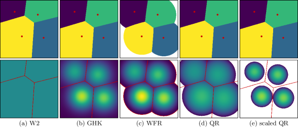
Figure 2: Semi-discrete transport between the Lebesgue measure on $\Omega=[0,L]^{2}$, $L=5$ and a discrete measure with $M=4$ Dirac masses of locations $(x_{1},x_{2},x_{3},x_{4})=L\cdot((0.375,0.375),(0.75,0.35),(0.65,0.75),(0.25,0.8))$ and weights $(m_{1},m_{2},m_{3},m_{4})=|\Omega|\cdot(0.38,0.29,0.19,0.14)$. Top row: optimal cells $\{C_{i}(w)\}_{i=1}^{M}$; the residual set $R$ is represented by white; location of the discrete points $(x_{1},\ldots,x_{M})$ is indicated with red dots. Bottom row: optimal marginal $\rho$ (identical colour scale in all figures; regions with $\tfrac{\textnormal{d}\rho}{\textnormal{d}\mu}(x)=0$ are white for emphasis) and boundaries of cells $\{C_{i}(w)\}_{i=1}^{M}$ (red) are shown for models (a)–(d) from Examples 2.8 and 3.13. Figure (e) shows the same model as (d), only with $c(x,y)=[d(x,y)/2]^{2}$ instead of $c(x,y)=d(x,y)^{2}$; on some cells $\operatorname{spt}\rho$ is now strictly bounded away from the boundaries of $C_{i}(w)$.

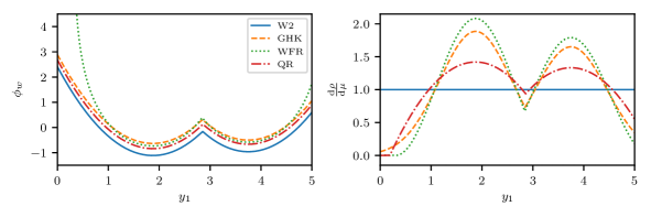
Figure 3: One-dimensional slices of computational results from Fig. 2 along $[0,L]\times\{0.375\,L\}$ with $L=5$. Left: $\phi_{w}$ for optimal $w\in\mathbb{R}^{M}$. For models (a), (b), and (d), $\phi_{w}$ is piecewise quadratic; for (c) the profile is determined by $c_{\textnormal{WFR}}$ and $\phi_{w}=\infty$ on $R\neq\emptyset$. Right: Optimal density $\tfrac{\textnormal{d}\rho}{\textnormal{d}\mu}$, where $\tfrac{\textnormal{d}\rho}{\textnormal{d}\mu}=(F^{\ast})^{\prime}(-\phi_{w})$ on $\Omega\setminus R$ and $0$ elsewhere by (3.4b). For (a) the density is constant, for (b) it is piecewise Gaussian, for (c) it is piecewise given by $\cos(d(y,x_{i}))^{2}$ on $\Omega\setminus R$ and $0$ on $R$, and for (d) it is given by truncated paraboloids.

Example 3.14 (Varying transport length scales).

As illustrated in the previous comparison of different models, unbalanced transport models typically have an intrinsic length scale which determines how far mass is optimally transported. Varying this length scale for fixed $\mu$ and $\nu$ changes the behaviour of the semi-discrete transport. For illustration we concentrate on the Wasserstein–Fisher–Rao distance and vary its intrinsic length scale by replacing $c(x,y)=c_{\textnormal{WFR}}(x,y)$ with

$$c(x,y)=c_{\textnormal{WFR}}^{\varepsilon}(x,y)=c_{\textnormal{WFR}}(\tfrac{x}{\varepsilon},\tfrac{y}{\varepsilon})=\begin{cases}-2\log\big{[}\cos\big{(}d(x,y)/\varepsilon\big{)}\big{]}&\textnormal{if }d(x,y)<\tfrac{\pi}{2}\varepsilon,\\ \infty&\textnormal{otherwise,}\end{cases}$$

that is, we set

$$\textnormal{WFR}^{\varepsilon}(\mu,\nu)^{2}=\\ \inf\left\{\int_{\Omega\times\Omega}c_{\textnormal{WFR}}^{\varepsilon}\textnormal{d}\gamma+\int_{\Omega}F_{\textnormal{KL}}\left(\tfrac{\textnormal{d}{\pi_{1}}_{\#}\gamma}{\textnormal{d}\mu}\right)\textnormal{d}\mu+\int_{\Omega}F_{\textnormal{KL}}\left(\tfrac{\textnormal{d}{\pi_{2}}_{\#}\gamma}{\textnormal{d}\nu}\right)\textnormal{d}\nu\,\middle|\,\gamma\in{\mathcal{M}_{+}}(\Omega\times\Omega)\right\}\,.$$

Note that this is equivalent to rescaling the domain $\Omega$ by the factor $\frac{1}{\varepsilon}$ and simultaneously replacing the measures $\mu$ and $\nu$ by their pushforwards under $x\mapsto\frac{x}{\varepsilon}$.

For large $\varepsilon$, transport becomes very cheap relative to mass changes and thus asymptotically, as $\varepsilon\to\infty$, one recovers the Wasserstein-2 distance: $\lim_{\varepsilon\to\infty}\varepsilon\textnormal{WFR}^{\varepsilon}(\mu,\nu)=W_{2}(\mu,\nu)$ by [33, Thm. 7.24]. In particular the distance diverges when $\mu(\Omega)\neq\nu(\Omega)$. Conversely, as $\varepsilon\searrow 0$, transport becomes increasingly expensive and mass change is preferred. Asymptotically one obtains $\lim_{\varepsilon\searrow 0}\textnormal{WFR}^{\varepsilon}(\mu,\nu)=\operatorname{Hell}(\mu,\nu)$ [33, Thm. 7.22], where $\operatorname{Hell}$ denotes the Hellinger distance

$$\operatorname{Hell}(\mu,\nu)^{2}=\int_{\Omega}\left(\sqrt{\tfrac{\textnormal{d}\mu}{\textnormal{d}\sigma}}-\sqrt{\tfrac{\textnormal{d}\nu}{\textnormal{d}\sigma}}\right)^{2}\textnormal{d}\sigma$$

for $\sigma\in{\mathcal{M}_{+}}(\Omega)$ an arbitrary reference measure with $\mu,\nu\ll\sigma$ (for instance $|\mu|+|\nu|$ with $|\cdot|$ indicating the total variation measure). By positive one-homogeneity of the function $(m_{1},m_{2})\mapsto(\sqrt{m_{1}}-\sqrt{m_{2}})^{2}$ the value of $\operatorname{Hell}(\mu,\nu)$ does not depend on the choice of $\sigma$. In our semi-discrete setting, $\mu$ and $\nu$ are always mutually singular so that $\operatorname{Hell}(\mu,\nu)^{2}=\mu(\Omega)+\nu(\Omega)$.

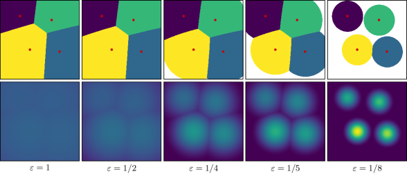
Figure 4: Semi-discrete Wasserstein–Fisher–Rao transport on $\Omega=[0,1]^{2}$ (using the same values for $x_{i}/L$ and $m_{i}/|\Omega|$ as in Fig. 2) for different length scales $\varepsilon$. Top row: optimal cells $\{C_{i}(w)\}_{i=1}^{M}$; the residual set $R$ is represented by white; location of the discrete points $(x_{1},\ldots,x_{M})$ is indicated with red dots. Bottom row: optimal marginal $\rho$ (using the same colour scale for all images). For large $\varepsilon$ the behaviour is similar to that of the standard semi-discrete Wasserstein-2 distance. As $\varepsilon$ decreases, the effects of unbalanced transport become increasingly prominent.

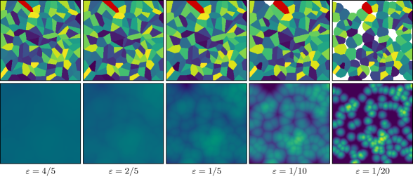
Figure 5: Semi-discrete Wasserstein–Fisher–Rao distance on $\Omega=[0,1]^{2}$ for different length scales $\varepsilon$, as in Fig. 4, but for $M=128$. The evolution of one cell $C_{i}(w)$ for fixed $i$ is highlighted in red (top row). For large $\varepsilon$, $C_{i}(w)$ is essentially the standard Wasserstein-2 Laguerre cell, not necessarily containing $x_{i}$. For small $\varepsilon$, $C_{i}(w)$ becomes (a fraction of) the open ball $B_{\varepsilon\pi/2}(x_{i})$.

Figure 4 illustrates the optimal cells $\{C_{i}(w)\}_{i=1}^{M}$ and marginal densities $\rho={\pi_{1}}_{\#}\gamma$ between the uniform volume measure $\mu=\mathcal{L}$ on $\Omega=[0,1]^{2}$ and a discrete measure $\nu=\sum_{i=1}^{M}m_{i}\,\delta_{x_{i}}$ for $M=4$, using different values of the intrinsic length scale $\varepsilon$ (the same experiment with $M=128$ discrete points is shown in Fig. 5). As expected, for large $\varepsilon$ the cells $\{C_{i}(w)\}_{i=1}^{M}$ look very similar to standard, polygonal Laguerre cells for the squared Euclidean distance $c(x,y)=d(x,y)^{2}$, and the residual set $R$ is empty. The optimal $\rho$ is essentially equal to $\mu$, as dictated by balanced transport. As $\varepsilon$ decreases, the boundaries between the cells become curved. Eventually $R$ becomes non-empty, and finally the cells start to decompose into disjoint discs. In accordance, the density of the optimal marginal $\rho$ is given on each cell $C_{i}(w)$ by $\cos(d(x,x_{i})/\varepsilon)^{2}\cdot e^{w_{i}}$. The interpolatory behaviour of $\textnormal{WFR}^{\varepsilon}$ between the Wasserstein-2 distance $W_{2}$ and the Hellinger distance $\operatorname{Hell}$ for $\varepsilon\to\infty$ and $\varepsilon\searrow 0$ is numerically verified in Fig. 6.

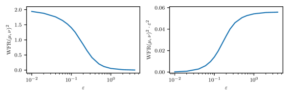
Figure 6: $\textnormal{WFR}^{\varepsilon}(\mu,\nu)^{2}$ for different length scales $\varepsilon$ for the setup from Fig. 4. Left: as $\varepsilon\searrow 0$, $\textnormal{WFR}^{\varepsilon}(\mu,\nu)^{2}$ tends to $\operatorname{Hell}(\mu,\nu)^{2}=2$. Right: as $\varepsilon\to\infty$, $\varepsilon^{2}\textnormal{WFR}^{\varepsilon}(\mu,\nu)^{2}$ tends to $W_{2}(\mu,\nu)^{2}$.

4 Unbalanced quantization

In this section we study the unbalanced quantization problem: we aim to approximate a given Lebesgue-continuous measure $\mu\in{\mathcal{M}_{+}}(\Omega)$ by a discrete, quantized measure $\nu=\sum_{i=1}^{M}m_{i}\cdot\delta_{x_{i}}$ with at most $M\in\mathbb{N}$ Dirac masses, where the unbalanced transport cost serves as a measure of approximation quality. To be precise, we consider the optimization problem

$$\min\left\{W(\mu,\nu)\,\middle|\,\nu=\sum_{i=1}^{M}m_{i}\delta_{x_{i}},\,x_{1},\ldots,x_{M}\in\Omega,\,m_{1},\ldots,m_{M}\geq 0\right\}\,.$$ (4.1)

Applications include optimal location problems (economic planning), information theory (vector quantization) and particle methods for PDEs (approximation of continuous initial data by particles). We first characterize optimal particle configurations in terms of Voronoi diagrams, then consider a corresponding numerical scheme, and finally prove the optimal energy scaling of the quantization problem in terms of $M$ for the case $d=2$. The procedure essentially follows the one known for classical optimal transport; the important fact is that the Voronoi tessellation structure survives if mass changes are allowed.

Throughout this section we will assume that zero mass change induces zero cost,

$$F(1)=0\,.$$ (4.2a)

This is the natural choice for approximating $$\mu {\pi_{1}}_{\#}\gamma=\mu \mathcal{F} F(z)\geq 0$$, as it implies a preference for in the first marginal fidelity term of (2.5). Since by Definition 2.2, a consequence is

$$0\in\partial F(1)\qquad\Leftrightarrow\qquad 1\in\partial F^{\ast}(0)\qquad\Leftrightarrow\qquad F^{\ast}(0)=0\,.$$ (4.2b)

4.1 Unbalanced quantization as a Voronoi tessellation problem

The existence of solutions to (4.1) follows from the direct method of the calculus of variations, noting that without loss of generality one may restrict to the compact search space $\Omega^{M}\times[0,\mu(\Omega)]^{M}$ (indeed, projecting the $m_{i}$ to $[0,\mu(\Omega)]$ decreases $W(\mu,\nu)$ due to assumption (4.2)) and that $W$ is weakly-$*$ lower semi-continuous in its arguments. The following theorem shows that the quantization problem can equivalently be formulated as an optimization of the points $x_{1},\ldots,x_{M}$ with a functional depending on the Voronoi tessellation induced by $(x_{1},\ldots,x_{M})$.

Theorem 4.1 (Tessellation formulation of quantization problem).

For $F$ satisfying (4.2), the unbalanced quantization problem (4.1) is equivalent to the minimization problem

$$\min\left\{J(x_{1},\ldots,x_{M})\,\middle|\,x_{1},\ldots,x_{M}\in\Omega\right\}$$ (4.3)

where

$$J(x_{1},\ldots,x_{M})=\sum_{i=1}^{M}\int_{V_{i}(x_{1},\ldots,x_{M})}-F^{\ast}(-c(x,x_{i}))\,\textnormal{d}\mu(x)$$

and where $V_{i}(x_{1},\ldots,x_{M})=\{x\in\Omega\,|\,d(x,x_{i})\leq d(x,x_{j})\text{ for }j=1,\ldots,M\,\}$ is the Voronoi cell associated with $x_{i}$ and we adopt the convention $-F^{\ast}(-\infty)=F(0)$ (cf. Lemma 2.9). Indeed, the minimum values coincide and, if $(x_{1},\ldots,x_{M})$ minimizes (4.3) and the minimal value is finite, then $(x_{1},\ldots,x_{M},m_{1},\ldots,m_{M})$ minimizes (4.1) for

$$m_{i}=\int_{V_{i}(x_{1},\ldots,x_{M})}\partial F^{\ast}(-c(x,x_{i}))\,\textnormal{d}\mu(x)\,,\quad i=1,\ldots,M.$$ (4.4)

(By the proof of Corollary 3.3 the subgradient $\partial F^{\ast}(-c(x,x_{i}))$ contains a unique element for $\mu$-almost every $x$ and so the $m_{i}$ are well defined.) Furthermore, the optimal transport plan $\gamma$ associated with $W(\mu,\nu)$ only transports mass from each Voronoi cell $V_{i}(x_{1},\ldots,x_{M})$ to the corresponding point $x_{i}$.

Example 4.2 (Tessellation formulation for unbalanced transport models).

The cost functional in (4.3) and the masses in (4.4) for the models from Example 2.8 are

$$\text{W2}: \begin{cases}\displaystyle J=\sum_{i=1}^{M}\int_{V_{i}}d(x,x_{i})^{2}\,\textnormal{d}\mu(x)\,,\\ \displaystyle m_{i}=\mu(V_{i})\,,\end{cases}$$

$$\text{GHK}: \begin{cases}\displaystyle J=\sum_{i=1}^{M}\int_{V_{i}}\left[1-e^{-d(x,x_{i})^{2}}\right]\,\textnormal{d}\mu(x)\,,\\ \displaystyle m_{i}=\int_{V_{i}}e^{-d(x,x_{i})^{2}}\,\textnormal{d}\mu(x)\,,\end{cases}$$

$$\text{WFR}: \begin{cases}\displaystyle J=\sum_{i=1}^{M}\int_{V_{i}}\sin^{2}\left(\min\left\{d(x,x_{i}),\tfrac{\pi}{2}\right\}\right)\,\textnormal{d}\mu(x)\,,\\ \displaystyle m_{i}=\int_{V_{i}}\cos^{2}\left(\min\left\{d(x,x_{i}),\tfrac{\pi}{2}\right\}\right)\,\textnormal{d}\mu(x)\,,\end{cases}$$

$$\text{QR}: \begin{cases}\displaystyle J=\sum_{i=1}^{M}\int_{V_{i}\cap B_{\sqrt{2}}(x_{i})}\left[d(x,x_{i})^{2}-\frac{d(x,x_{i})^{4}}{4}\right]\,\textnormal{d}\mu(x)+\mu(V_{i}\setminus B_{\sqrt{2}}(x_{i}))\,,\\ \displaystyle m_{i}=\int_{V_{i}}\max\left\{1-\frac{d(x,x_{i})^{2}}{2},0\right\}\,\textnormal{d}\mu(x).\end{cases}$$

Remark 4.3.

An intuitive strategy for proving Theorem 4.1 could be as follows. One starts from the primal tessellation formulation in Corollary 3.5 and in addition minimizes over masses $(m_{1},\ldots,m_{M})$ and positions $(x_{1},\ldots,x_{M})$. By (4.2) we find that minimizing masses are given by $m_{i}=\rho(C_{i}(w))$. Next, only the transport term depends on the weights $w$, and since the cost $c$ is a strictly increasing function of distance, the term is minimized for $w=0$, thus essentially reducing the generalized Laguerre cells $C_{i}(w)$ into (truncated) Voronoi cells. Finally, the remaining minimization over $\rho$ can be handled with arguments from convex analysis, similar to those of Theorem 3.2, thus arriving at (4.3). We give a shorter proof, using results from the dual tessellation formulation and its optimality conditions.

Proof of Theorem 4.1.

Let $\nu=\sum_{i=1}^{M}m_{i}\cdot\delta_{x_{i}}$ be any admissible measure for (4.1). From (3.1b) we find $W(\mu,\nu)\geq\mathcal{G}(0)$ for any positions $x_{1},\ldots,x_{M}$ and masses $m_{1},\ldots,m_{M}$. Note that $\mathcal{G}(0)$ does not depend on $m_{1},\ldots,m_{M}$ since we assume $F^{\ast}(0)=0$, (4.2b). We now show $W(\mu,\nu)=\mathcal{G}(0)$ for a particular choice of $m_{1},\ldots,m_{M}$, which therefore must be optimal (for given locations $x_{1},\ldots,x_{M}$). We first define $\rho$ via (3.4b) and then $\gamma$ via (3.4a) for $w=0$ ($\rho$ and $\gamma$ are fully determined, see Corollary 3.3). Furthermore, since $1\in\partial F^{\ast}(0)$ by (4.2b), equation (3.4c) is satisfied by the choice $m_{i}=\rho(C_{i}(0))$. By Theorem 3.2, $\gamma$ and $w$ are optimizers of $\mathcal{E}$ and $\mathcal{G}$ for these mass coefficients, which implies that $W(\mu,\nu)=\mathcal{G}(0)$. Using $F^{\ast}(0)=0$ from (4.2b), we have

$$\min_{(m_{1},\ldots,m_{M})}W(\mu,\nu)=\mathcal{G}(0)=-\sum_{i=1}^{M}\int_{C_{i}(0)}F^{\ast}\big{(}-c(x,x_{i})\big{)}\,\textnormal{d}\mu(x)+F(0)\cdot\mu(R)\,.$$

Since $c(x,y)$ is a strictly increasing function of the distance $d(x,y)$, for $w=0$ we find $C_{i}(0)\subset V_{i}(x_{1},\ldots,x_{M})$. With the convention $-F^{\ast}(-\infty)=F(0)$ (cf. Lemma 2.9), the term $F(0)\cdot\mu(R)$ becomes $\int_{R}-F^{\ast}(-\phi_{0}(x))\,\textnormal{d}\mu(x)$, where $\phi_{0}$ was defined in equation (2.13). Since $\mu\ll\mathcal{L}$, integrating over $R$ and $\Omega\setminus R$ is equivalent to integrating over all Voronoi cells $\{V_{i}(x_{1},\ldots,x_{M})\}_{i=1}^{M}$, and we arrive at

$$\min_{(m_{1},\ldots,m_{M})}W(\mu,\nu)=-\sum_{i=1}^{M}\int_{V_{i}(x_{1},\ldots,x_{M})}F^{\ast}\big{(}-c(x,x_{i})\big{)}\,\textnormal{d}\mu(x)\,,$$

which establishes equivalence between (4.1) and (4.3).

Finally, with $m_{i}=\rho(C_{i}(0))$ and $\rho$ given by (3.4b) one obtains (4.4), where the integral runs over $C_{i}(0)$ instead of $V_{i}(x_{1},\ldots,x_{M})$. If the minimum is finite, then either $\mu(R)=0$ or $F(0)$ is finite, which implies the convention $(F^{\ast})^{\prime}(-\infty)=0$ (cf. Lemma 2.9(vii)). In both cases we can extend the area of integration to $V_{i}(x_{1},\ldots,x_{M})$ without changing its value. Equation (3.4a) implies that mass is only transported from each Voronoi cell $V_{i}(x_{1},\ldots,x_{M})\supset C_{i}(0)$ to the corresponding point $x_{i}$. ∎

4.2 A numerical method: Lloyd’s algorithm and quasi-Newton variant

Formulation (4.3) has the advantage over (4.1) that it does not contain an inner minimization to find the optimal transport coupling. Thus we aim to solve (4.3) numerically. To this end we compute the gradient $\partial_{x_{j}}J$ (see also analogous derivatives for similar functionals as for instance in [9]).

Lemma 4.4 (Derivative of the cost functional $J$).

Let $\mu\in{\mathcal{M}_{+}}(\Omega)$ be Lebesgue-continuous, and let $F^{\ast}\circ(-\ell)$ be Lipschitz continuous on $[0,\mathrm{diam}(\Omega)]$. Then for $j=1,\ldots,M$,

$$\partial_{x_{j}}J(x_{1},\ldots,x_{M})=\int_{V_{j}(x_{1},\ldots,x_{M})}r(d(x,x_{j}))(x_{j}-x)\,\textnormal{d}\mu(x)$$

where

$$r(s)=\frac{[-F^{\ast}\circ(-\ell)]^{\prime}(s)}{s}$$

(note that $-F^{\ast}\circ(-\ell)$ is differentiable for almost every $s\in[0,\mathrm{diam}(\Omega)]$ so that $r$ and $r(d(\cdot,x_{j}))$ are well-defined almost everywhere).

Example 4.5 (Cost derivative for unbalanced transport models).

For the models from Example 2.8 one can readily check

$$\text{W2}: r(s)=2\,,$$

$$\text{GHK}: r(s)=2e^{-s^{2}}\,,$$

$$\text{WFR}: r(s)=\sin(2s)/s\text{ if }s\leq\tfrac{\pi}{2}\text{ and }0\text{ otherwise,}$$

$$\text{QR}: r(s)=\max\{2-s^{2},0\}\,.$$

Proof.

Note that $J(x_{1},\ldots,x_{M})=\int_{\Omega}f(x,(x_{1},\ldots,x_{M}))\,\textnormal{d}\mu(x)$ with

$$f(x,(x_{1},\ldots,x_{M}))=\min\{-F^{\ast}(-\ell(d(x,x_{i})))\,|\,i=1,\ldots,M\}\,$$

since $F^{\ast}$ and $l$ are increasing. By assumption on $F^{\ast}\circ(-\ell)$, $f$ is Lipschitz in its second argument. Furthermore, $F^{\ast}\circ(-\ell)$ is differentiable almost everywhere, and $d(x,x_{i})$ is differentiable in its second argument for all $x\neq x_{i}$. Therefore, $f$ is differentiable in its second argument at $(x_{1},\ldots,x_{M})$ for almost all $x\in\Omega$ (thus for $\mu$-almost all $x\in\Omega$) with

$$\partial_{x_{j}}f(x,(x_{1},\ldots,x_{M}))=\begin{cases}r(d(x,x_{j}))(x_{j}-x)&\text{if }x\in V_{j}(x_{1},\ldots,x_{M}),\\ 0&\text{otherwise.}\end{cases}$$

Lemma 3.8 now implies the desired result. ∎

To find a minimizer of $J$ and thus a solution to the optimality condition $\partial_{x_{j}}J=0$ for $j=1,\ldots,M$, one can perform the following fixed point iteration associated with the optimality conditions,

$$x_{i}^{(k+1)}=\frac{\displaystyle\int_{V_{i}(x_{1}^{(k)},\ldots,x_{M}^{(k)})}xr(d(x_{i}^{(k)},x))\,\textnormal{d}\mu(x)}{\displaystyle\int_{V_{i}(x_{1}^{(k)},\ldots,x_{M}^{(k)})}r(d(x_{i}^{(k)},x))\,\textnormal{d}\mu(x)}\,,\quad i=1,\ldots,M,$$

starting from some initialization $x_{1}^{(0)},\ldots,x_{M}^{(0)}\in\Omega$. This iteration is well-defined as long as the denominator is nonzero, for instance if $\mu$ is strictly positive on $\Omega$. This is a generalisation of Lloyd’s algorithm for computing Centroidal Voronoi Tessellations [15], which are critical points of the function

$$\tilde{J}(x_{1},\ldots,x_{M})=\sum_{i=1}^{M}\int_{V_{i}(x_{1},\ldots,x_{M})}|x-x_{i}|^{2}\,\textnormal{d}\mu(x)\,.$$

Its convergence has been proven in a number of settings [44, 18, 9] which also cover many possible choices for our $\mu$, $c$, and $F$. Since the algorithm is based solely on the first variation one can expect linear convergence. To achieve faster convergence one may use a quasi-Newton method for the minimization of $J$ instead, which seems particularly well-suited since the optimization is performed over a finite-dimensional space.

Our numerical implementation is performed in Matlab. The integrals over a Voronoi cell $V_{i}(x_{1},\ldots,x_{M})$ are evaluated using Gaussian quadrature on the triangulation which is obtained by connecting each vertex of $V_{i}(x_{1},\ldots,x_{M})$ with $x_{i}$. The Voronoi cells themselves are computed using the built-in function voronoin. Figure 7 shows a slightly faster convergence of the BFGS method compared to Lloyd’s algorithm, while Fig. 8 shows quantization results for the same models as in Fig. 2, resulting in different point distributions. Similarly, Fig. 9 shows quantization results for the same input marginal $\mu$ and the Wasserstein–Fisher–Rao model, but for varying length scales.

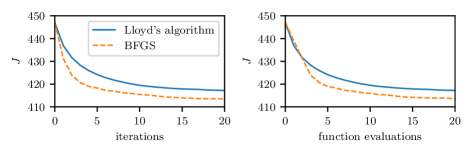
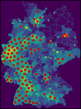
Figure 7: Quantization energy decrease of Lloyd’s algorithm and a BFGS method versus number of iterations (left) and function evaluations (centre) for the example shown on the right. Right: Input density $\mu$ and optimal locations $(x_{1},\ldots,x_{M})$ for $M=100$, where $\mu$ is population density in Germany 2015 (published by the Federal Statistical Office of Germany in the “Regional Atlas” http://www.destatis.de/regionalatlas). The computations use the Wasserstein–Fisher–Rao model.

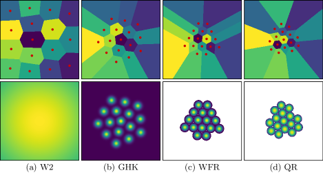
Figure 8: Quantization results for $\mu=(1+\exp(-\frac{|x|^{2}}{2(4\pi)^{2}}))\cdot\mathcal{L}{\mbox{\LARGE$\llcorner$}}\Omega$ and $\Omega=[-4\pi,4\pi]^{2}$, $M=16$ on the same models as in Fig. 2. Top row: optimal locations $x_{1},\ldots,x_{M}$ and Voronoi cells $\{V_{i}(x_{1},\ldots,x_{M})\}_{i=1}^{M}$. Bottom row: optimal marginal $\rho={\pi_{1}}_{\#}\gamma$ (identical colour scale in all figures; regions with $\tfrac{\textnormal{d}\rho}{\textnormal{d}\mu}(x)=0$ are white for emphasis). For (a) we have $\rho=\mu$.

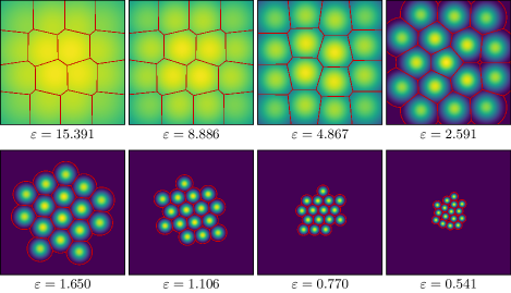
Figure 9: Quantization results for the Wasserstein–Fisher–Rao model and different length scales, showing the optimal Voronoi cells and the optimal marginals $\rho={\pi_{1}}_{\#}\gamma$ (same domain and $\mu$ as in Fig. 8; identical colour scale in all figures).

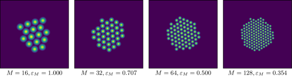
Figure 10: Quantization results for the Wasserstein–Fisher–Rao model using different length scales and numbers of discrete points, with constant total point density $\varepsilon_{M}^{2}M$. The optimal marginals $\rho={\pi_{1}}_{\#}\gamma$ are shown (same domain and $\mu$ as in Fig. 8; identical colour scale in all figures).

4.3 Crystallization in two dimensions

In this section we consider the asymptotic behaviour of the unbalanced quantization problem in the limit of infinitely many points, $M\to\infty$, in two dimensions, $\Omega\subset\mathbb{R}^{2}$, in which case crystallization results from discrete geometry are available.

To simplify the exposition in this section we assume

$$0<F(0)<+\infty$$ (4.5a)

so that the unbalanced transport cost is always finite. (The inequality $$0<F(0)$$ simply ensures that the quantization problem is not trivially degenerate.) These two inequalities imply

$$F^{\ast}(z)\leq 0\textnormal{ for }z<0\qquad\textnormal{and}\qquad F^{\ast}(z)\geq-F(0)\textnormal{ for }z\in\mathbb{R}.$$ (4.5b)

The case $F(0)=\infty$ can in principle be treated similarly, but requires a number of technical case distinctions (such as whether the domain of $(-F^{\ast}\circ(-\ell))$ is open or closed, whether $0$ is in the domain closure or not, etc.).

As we increase $M$, the average distance between points of $\Omega$ and their nearest discrete point $x_{i}$ decreases so that the (balanced) transport cost from $\mu$ onto $\nu$ vanishes in the limit, whereas the cost for changing mass remains unchanged. Therefore, in the limit $M\to\infty$ the interplay of transport and mass change in unbalanced transport would not be visible. To avoid this, we will rescale the metric on the domain $\Omega$ as $M$ grows and study the resulting different regimes, depending on the scaling. Consequently, in this section we consider the scaled cost

$$J_{\varepsilon}^{M}(x_{1},\ldots,x_{M})=\sum_{i=1}^{M}\int_{V_{i}(x_{1},\ldots,x_{M})}-F^{\ast}\left(-\ell\left(\tfrac{d(x,x_{i})}{\varepsilon}\right)\right)\,\textnormal{d}\mu(x)$$ (4.6)

for $M\in\mathbb{N}$, $\varepsilon\in(0,\infty)$.

We first prove a lower bound on the quantization cost $J_{\varepsilon}^{M}$ for the Lebesgue measure, which corresponds to a perfect triangular lattice. Then a corresponding upper bound is derived. Finally, for $\mu$ with Lipschitz continuous Lebesgue density, we show that these two bounds imply that asymptotically a regular triangular lattice becomes an optimal quantization configuration, where the local density of points depends on the density of $\mu$.

Theorem 4.6 (Lower bound for quantization of the Lebesgue measure).

Let $\Omega\subset\mathbb{R}^{2}$ be a convex polygon with at most six sides, and let $\mu$ be the Lebesgue measure on $\Omega$. A lower bound on (4.6) is given by

$$\min_{x_{1},\ldots,x_{M}\in\Omega}J_{\varepsilon}^{M}(x_{1},\ldots,x_{M})\geq M\int_{H(|\Omega|/M)}-F^{\ast}\left(-\ell\left(\tfrac{d(x,0)}{\varepsilon}\right)\right)\,\textnormal{d}x\,,$$ (4.7)

where $H(|\Omega|/M)$ is a regular hexagon of area $|\Omega|/M=\mathcal{L}(\Omega)/M$ centred at the origin $0$.

Remark 4.7 (Cost of the triangular lattice).

Comparing with Theorem 4.1, the lower bound is exactly the unbalanced transportation cost $W(\mu,\nu)$ from a regular triangular lattice $\nu$ of $M$ Dirac measures of mass

$$m=\int_{H(|\Omega|/M)}\partial F^{\ast}\left(-\ell\left(\tfrac{d(x,0)}{\varepsilon}\right)\right)\,\textnormal{d}x\,,$$

whose Voronoi cells are translations of $H(|\Omega|/M)$, onto $\mu$ the Lebesgue measure on the union of these Voronoi cells.

Proof of Theorem 4.6.

First observe that $-F^{\ast}(-\ell(\cdot/\varepsilon))$ is increasing since both $\ell$ and $F^{\ast}$ are increasing. Thus, for $x_{1},\ldots,x_{M}\in\Omega$ we have

$$J_{\varepsilon}^{M}(x_{1},\ldots,x_{M}) =\sum_{i=1}^{M}\int_{V_{i}(x_{1},\ldots,x_{M})}-F^{\ast}\left(-\ell\left(\tfrac{d(x,x_{i})}{\varepsilon}\right)\right)\,\textnormal{d}x$$

$$=\int_{\Omega}\min_{i=1,\ldots,M}-F^{\ast}\left(-\ell\left(\tfrac{d(x,x_{i})}{\varepsilon}\right)\right)\,\textnormal{d}x\,,$$

and the result follows immediately from L. Fejes Tóth’s Theorem on Sums of Moments [25] (see also [49, 38]). ∎

Remark 4.8 (Degeneracy of minimizers).

As opposed to the quantization problem for classical optimal transport, the set of minimizers in the unbalanced transport case can exhibit strong degeneracies. As an example, consider the case of Wasserstein–Fisher–Rao transport with $M\ll 4\,|\Omega|/(\pi^{3}\varepsilon^{2})$. Let $x_{1},\ldots,x_{M}$ be any arrangement of the point masses such that the balls $B_{\varepsilon\,\pi/2}(x_{i})$ are pairwise disjoint and included in $\Omega$ (which necessarily implies $M\leq 4\,|\Omega|/(\pi^{3}\varepsilon^{2})$). Then $(x_{1},\ldots,x_{M})$ achieves the lower bound since

$$J_{\varepsilon}^{M}(x_{1},\ldots,x_{M}) =\sum_{i=1}^{M}\int_{V_{i}(x_{1},\ldots,x_{M})}-F^{\ast}\left(-\ell\left(\tfrac{d(x,x_{i})}{\varepsilon}\right)\right)\,\textnormal{d}x$$

$$=\sum_{i=1}^{M}\int_{V_{i}(x_{1},\ldots,x_{M})}\sin^{2}\left(\min\left\{d(x,x_{i})/\varepsilon,\tfrac{\pi}{2}\right\}\right)\,\textnormal{d}x$$

$$=|\Omega|-M\varepsilon^{2}\,\pi^{3}/4+\sum_{i=1}^{M}\int_{B_{\varepsilon\,\pi/2}(x_{i})}\sin^{2}\left(d(x,x_{i})/\varepsilon\right)\,\textnormal{d}x$$

$$=M\int_{H(|\Omega|/M)}-F^{\ast}(-\ell(d(x,0)/\varepsilon))\,\textnormal{d}x\,,$$

where we used $H(|\Omega|/M)\supset B_{\varepsilon\,\pi/2}(0)$.

Theorem 4.9 (Upper bound for quantization of the Lebesgue measure).

Let $\Omega\subset\mathbb{R}^{2}$ be convex and let $\mu$ be the Lebesgue measure. Let $x_{1},\ldots,x_{M}$ be a regular triangular arrangement of points in the following sense: Let $G\subset\mathbb{R}^{2}$ be a regular triangular lattice with lattice spacing $\sqrt{\frac{2\,|\Omega|}{\sqrt{3}\,M}}$, such that the corresponding Voronoi cells are regular hexagons with area $|\Omega|/M$ and side length $L=\sqrt{\frac{2\,|\Omega|}{3\sqrt{3}M}}$. Let $\{x_{1},\ldots,x_{\hat{M}}\}\subset G$ be those points for which the corresponding hexagon $H_{i}$ is fully contained in $\Omega$. If $\hat{M}<M$, pick $\{x_{\hat{M}+1},\ldots,x_{M}\}$ arbitrarily from $\Omega$. Then

$$J_{\varepsilon}^{M}(x_{1},\ldots,x_{M})\leq M\int_{H(|\Omega|/M)}-F^{\ast}\left(-\ell\left(\tfrac{d(x,0)}{\varepsilon}\right)\right)\,\textnormal{d}x+F(0)\cdot|\partial\Omega|\sqrt{\frac{8|\Omega|}{3\sqrt{3}M}}\,,$$ (4.8)

where $|\partial\Omega|$ denotes the one-dimensional Hausdorff measure of $\partial\Omega$ and $|\Omega|=\mathcal{L}(\Omega)$.

Proof.

Let $S=\Omega\setminus\bigcup_{i=1}^{\hat{M}}H_{i}$ be those points in $\Omega$ that are not covered by any hexagon $H_{i}$. Note that all $x\in S$ lie no further away from $\partial\Omega$ than the diameter of a hexagon, $2L=\sqrt{\frac{8\,|\Omega|}{3\sqrt{3}M}}$. Since $\Omega$ is convex we thus have $|S|\leq|\Omega\cap\bigcup_{x\in\partial\Omega}B_{2L}(x)|\leq 2\,L\,|\partial\Omega|$.

Note that $V_{i}(x_{1},\ldots,x_{M})\setminus S\subseteq H_{i}$ for $i=1,\ldots,\hat{M}$ and $-F^{\ast}(-c(x,x_{i}))\leq-F^{\ast}(-\infty)\leq F(0)$ for any $i\in 1,\ldots,M$. Then we find

$$J_{\varepsilon}^{M}(x_{1},\ldots,x_{M}) \leq\sum_{i=1}^{\hat{M}}\int_{H_{i}}-F^{\ast}\left(-\ell\left(\tfrac{d(x,x_{i})}{\varepsilon}\right)\right)\,\textnormal{d}x+|S|\cdot F(0)$$

$$\leq M\cdot\int_{H(|\Omega|/M)}-F^{\ast}\left(-\ell\left(\tfrac{d(x,0)}{\varepsilon}\right)\right)\,\textnormal{d}x+|S|\cdot F(0)\,.$$

Substituting the above bound for $|S|$ proves the claim. ∎

Remark 4.10 (A priori estimate).

Since $-F^{\ast}\circ(-\ell)$ is increasing and $F^{\ast}\geq-F(0)$ we also have the estimate

$$\min J_{\varepsilon}^{M}\leq\int_{\Omega}-F^{\ast}(-\ell(\infty))\,\textnormal{d}\mu\leq\mu(\Omega)\cdot F(0)=W(\mu,0)\,.$$

Let now $(\varepsilon_{M})_{M\in\mathbb{N}}$ be a positive, decreasing sequence of scaling factors. We use Theorems 4.6 and 4.9 to study the asymptotic quantization behaviour of the sequence of functionals $(J_{\varepsilon_{M}}^{M})_{M}$ as $M\to\infty$ for a non-uniform mass distribution $\mu$ with Lipschitz Lebesgue density $m$. We identify three different regimes, depending on the behaviour of the sequence $\varepsilon_{M}^{2}\,M$ (the quantity $\varepsilon_{M}^{2}\,M$ indicates something like the average point density). A corresponding numerical illustration for the case of constant average point density is provided in Fig. 10.

Before stating the asymptotic result we need to analyse the cell problem of quantizing a hexagon by a single Dirac mass.

Lemma 4.11 (Properties of the cell problem).

Assume that $\lim_{s\to\infty}\ell(s)=\infty$. Define $B:(-\infty,\infty)\to(0,\infty]$ by

$$B(z)=z\cdot\int_{H(1/z)}-F^{\ast}(-\ell(d(x,0)))\,\textnormal{d}x\,\quad\textnormal{for }z>0,$$

$B(0)=F(0)$, $B(z)=\infty$ for $z<0$. Then, on $(0,\infty)$, $B$ is nonnegative, nonincreasing, and convex with continuous derivative

$$B^{\prime}(z)=\frac{1}{z}\left[B(z)-\tfrac{1}{|\partial H(1/z)|}\int_{\partial H(1/z)}-F^{\ast}(-\ell(d(x,0)))\,\textnormal{d}x\right]\,=:G(z).$$

Furthermore, $B(z)\to F(0)$ as $z\searrow 0$, while $B(z)\to 0$ and $B^{\prime}(z)\to 0$ as $z\to\infty$. Also, there exists some $Z\geq 0$ such that $B^{\prime}$ is constant on $(0,Z]$ and strictly increasing on $(Z,\infty)$. With $r=\lim_{z\searrow Z}B^{\prime}(z)$ we can summarize $r<G(z)<0$ for $z>Z$ and

$$\partial B(z)=\begin{cases}\emptyset&\textnormal{ for }z<0,\\ (-\infty,r]&\textnormal{ for }z=0,\\ \{r\}&\textnormal{ for }z\in(0,Z],\\ \{G(z)\}&\textnormal{ for }z>Z,\end{cases}\qquad\partial(B^{\ast})(s)=\begin{cases}\{0\}&\textnormal{ for }s<r,\\ [0,Z]&\textnormal{ for }s=r,\\ \{G^{-1}(s)\}&\textnormal{ for }s\in(r,0),\\ \emptyset&\textnormal{ for }s\geq 0.\end{cases}$$

Example 4.12 (Balanced quantization).

The results of Lemma 4.11 hold even if $F$ does not satisfy assumption (4.5a). We consider the case of the standard Wasserstein-2 distance, where $\ell(t)=t^{2}$, $F^{\ast}(z)=z$ and $F(0)=\infty$. Then for $z>0$,

$$B(z)=z\int_{H(1/z)}|x|^{2}\textnormal{d}x=\frac{5\sqrt{3}}{54}\frac{1}{z},\qquad B^{\prime}(z)=G(z)=-\frac{5\sqrt{3}}{54}\frac{1}{z^{2}}.$$

and so $Z=0$, $r=-\infty$. For $s<0$,

$$B^{\ast}(s)=-2\sqrt{-\frac{5\sqrt{3}}{54}\,s},\qquad(B^{\ast})^{\prime}(s)=\sqrt{-\frac{5\sqrt{3}}{54}\frac{1}{s}}=G^{-1}(s).$$

Remark 4.13.

$B(z)$ can be interpreted as energy density associated with a regular triangular lattice with point density $z$ (that is, each Voronoi cell occupies an area of $1/z$). The energy of such a lattice with $M$ cells with total area $|\Omega|$ will be given by $B(M/|\Omega|)\cdot|\Omega|$. Taking into account the scaling factor $\varepsilon$, we can restate the bounds (4.7) and (4.8) as

$$\min_{x_{1},\ldots,x_{M}\in\Omega}J_{\varepsilon}^{M}(x_{1},\ldots,x_{M}) \geq|\Omega|\cdot B\big{(}\tfrac{\varepsilon^{2}\,M}{|\Omega|}\big{)}\qquad\textnormal{and}$$

$$J_{\varepsilon}^{M}(x_{1},\ldots,x_{M}) \leq|\Omega|\cdot B\big{(}\tfrac{\varepsilon^{2}\,M}{|\Omega|}\big{)}+F(0)\cdot|\partial\Omega|\sqrt{\frac{8|\Omega|}{3\sqrt{3}M}}.$$

Proof of Lemma 4.11.

By (4.5b), $-F^{\ast}(-\ell(d(x,0)))>0$ for $x\neq 0$, therefore $B(z)>0$ for $z>0$. Also by (4.5b), $F^{\ast}$ is bounded from below, so $B(z)<\infty$. $B$ is nonincreasing since $-F^{\ast}\circ(-\ell)$ is nondecreasing. Now observe that $B$ yields the average value of $-F^{\ast}(-\ell(d(\cdot,0)))$ over $H(1/z)$,

$$B(z)=-F^{\ast}(-\ell(d(\xi(z),0)))$$

for some $\xi(z)\in H(1/z)$. Therefore $\lim_{z\to\infty}B(z)=-F^{\ast}(-\ell(0))=-F^{\ast}(0)=0$ by (4.2b). Conversely,

$$\lim_{z\searrow 0}\,B(z)=\lim_{z\searrow 0}\,\int_{H(1)}-F^{\ast}(-\ell(d(y/\sqrt{z},0)))\,\textnormal{d}y=-F^{\ast}(-\ell(\infty))=-F^{\ast}(-\infty)=F(0).$$

Since $-F^{\ast}\circ(-\ell)$ is continuous, the integral in the definition of $B$ is differentiable with respect to $z$ by the Leibniz integral rule, and we have

$$B^{\prime}(z) =\frac{\textnormal{d}}{\textnormal{d}z}\left[z\int_{H(1/z)}-F^{\ast}(-\ell(d(x,0)))\,\textnormal{d}x\right]$$

$$=\int_{H(1/z)}-F^{\ast}(-\ell(d(x,0)))\,\textnormal{d}x+z\int_{\partial H(1/z)}-F^{\ast}(-\ell(d(x,0)))v_{n}(z)\,\textnormal{d}x\cdot\left(-\frac{1}{z^{2}}\right)\,,$$

where $v_{n}(z)=1/|\partial H(1/z)|$ is the normal velocity of the hexagonal boundary as the area of the hexagon is increased at rate $1$. This coincides with the formula provided in the statement. To check convexity we first assume that $-F^{\ast}\circ(-\ell)$ is differentiable. In the following we use the notation

$$-\int_{\partial H(1/z)}f\,\textnormal{d}x=\frac{1}{|\partial H(1/z)|}\int_{\partial H(1/z)}f\,\textnormal{d}x$$

and calculate

$$B^{\prime\prime}(z)=$$

$$=-\frac{1}{z^{2}}\left[B(z)--\int_{\partial H(1/z)}-F^{\ast}(-\ell(d(x,0)))\,\textnormal{d}x\right]$$

$$\quad+\frac{1}{z}\left[\frac{1}{z}\left(B(z)--\int_{\partial H(1/z)}-F^{\ast}(-\ell(d(x,0)))\,\textnormal{d}x\right)-\frac{\textnormal{d}}{\textnormal{d}z}\left(-\int_{\partial H(1/z)}-F^{\ast}(-\ell(d(x,0)))\,\textnormal{d}x\right)\right]$$

$$=-\frac{1}{z}\frac{\textnormal{d}}{\textnormal{d}z}\left(-\int_{\partial H(1/z)}-F^{\ast}(-\ell(d(x,0)))\,\textnormal{d}x\right)$$

$$\geq 0\$$

since $-F^{\ast}\circ(-\ell)$ is nondecreasing. Therefore $B$ is convex. Since $F^{\ast}$ is nondecreasing and convex, there exists some $R\in(0,\infty]$ such that $-F^{\ast}\circ(-\ell)$ is strictly increasing on $[0,R)$ and constant on $[R,\infty)$. Thus we see $B^{\prime\prime}>0$ on $(Z,\infty)$ for some $Z\geq 0$ and $B^{\prime\prime}(z)=0$ for $z<Z$. The monotonicity properties of $B^{\prime}$ without assuming differentiability of $-F^{\ast}\circ(-\ell)$ now follow by a standard approximation argument. Note that

$$0\geq B^{\prime}(z)\geq-\frac{1}{z}-\int_{\partial H(1/z)}-F^{\ast}(-\ell(d(x,0)))\,\textnormal{d}x\to 0\qquad\text{as }z\to\infty.$$

We leave it as an easy exercise in convex analysis to check the expressions for the subdifferentials $\partial B$ and $\partial(B^{\ast})$. ∎

Theorem 4.14 (Asymptotic quantization).

Let $\Omega\subset\mathbb{R}^{2}$ be a closed Lipschitz domain (a domain whose boundary is locally the graph of a Lipschitz function with the domain lying on one side) and $\mu=m\cdot(\mathcal{L}{\mbox{\LARGE$\llcorner$}}\Omega)$ for $\mathcal{L}$ the Lebesgue measure and $m:\Omega\to[0,\infty)$ a Lipschitz-continuous density. Furthermore, let $F(0)<\infty$ and $\lim_{s\to\infty}\ell(s)=\infty$. For any sequence $\varepsilon_{1},\varepsilon_{2},\ldots>0$ with $\varepsilon_{M}\searrow 0$ as $M\to\infty$ the following holds:

1. If $\displaystyle\lim_{M\to\infty}\varepsilon_{M}^{2}M=\infty$, then $\displaystyle\lim_{M\to\infty}\min J_{\varepsilon_{M}}^{M}=0$.

2. If $\displaystyle\lim_{M\to\infty}\varepsilon_{M}^{2}M=0$, then $\displaystyle\lim_{M\to\infty}\min J_{\varepsilon_{M}}^{M}=W(\mu,0)=\mu(\Omega)F(0)$.

3. If $\displaystyle\lim_{M\to\infty}\varepsilon_{M}^{2}M=P\in(0,\infty)$, then

   $$\lim_{M\to\infty}\min J_{\varepsilon_{M}}^{M}=\left[\kappa\mapsto\int_{\Omega}B^{\ast}(\kappa/m(x))\,\textnormal{d}\mu(x)\right]^{\ast}(P)\,.$$

   Furthermore, there exists a unique constant $\lambda<0$ and some measurable function $D:\Omega\to[0,\infty)$ such that

   $$\lim_{M\to\infty}\min J_{\varepsilon_{M}}^{M}=\int_{\Omega}B(D(x))\,\textnormal{d}\mu(x)\,,$$

   and

   $$D(x)\in\partial B^{\ast}(\lambda/m(x))\text{ for almost all }x\in\Omega,\qquad P=\int_{\Omega}D(x)\,\textnormal{d}x$$ (4.9)

   (by convention, for $m(x)=0$ we set $D(x)=0$). That is, $D$ can be interpreted as (being proportional to) the density of the asymptotically optimal point distributions.

Remark 4.15 (Limit cases).

Theorem 4.14(1) and (2) can in fact be recovered as the special cases $P=\infty$ and $P=0$ of Theorem 4.14(3) if we set $(\lambda,D)\equiv(0,\infty)$ or $(\lambda,D)\equiv(-\infty,0)$, respectively. However, it is simpler to treat them separately.

Remark 4.16 (Calculation of asymptotic density).

Given a density $m$, the asymptotically optimal point density $D$ can be computed numerically based on the function $B$ using

$$D(x)\in\partial B^{\ast}(\lambda/m(x))=\begin{cases}\{0\}&\text{if }\lambda/m(x)<r,\\ [0,Z]&\text{if }\lambda/m(x)=r,\\ \{(B^{\prime})^{-1}(\lambda/m(x))\}&\text{if }\lambda/m(x)\in(r,0),\\ \emptyset&\text{otherwise,}\end{cases}$$

where $r$ was defined in Lemma 4.11.

Example 4.17 (Balanced asymptotic quantization).

We consider the case of the standard Wasserstein-2 distance, where $\ell(t)=t^{2}$, $F^{\ast}(z)=z$ and $F(0)=\infty$, even if this does not satisfy assumption (4.5a). Let $m=1$ so that $\mu$ is the Lebesgue measure. Assume that we are in Regime 3. Then it is easy to check from the previous remark and Example 4.12 that

$$D(x)=\sqrt{-\frac{5\sqrt{3}}{54}\frac{1}{\lambda}},\qquad P=|\Omega|\sqrt{-\frac{5\sqrt{3}}{54}\frac{1}{\lambda}}.$$

Eliminating the unknown $\lambda$ gives

$$D(x)=\frac{P}{\Omega}.$$

Combining this with the expression for $B$ from Example 4.12 gives

$$\lim_{M\to\infty}\min J_{\varepsilon_{M}}^{M}=\frac{5\sqrt{3}}{54}\,\frac{|\Omega|^{2}}{P}.$$

If we take $\varepsilon^{2}_{M}=1/M$, $P=1$, $|\Omega|=1$, then this reduces to the classical asymptotic quantization result for the Wasserstein-2 distance; see, e.g., [8, Thm. 5].

Proof of Theorem 4.14.

Regime 1: $\lim_{M\to\infty}\varepsilon_{M}^{2}M=\infty$. Since $\Omega$ is a Lipschitz domain, for any $M\in\mathbb{N}$ we can cover $\Omega$ with $M$ balls of radius $r_{M}$ such that $M\cdot r_{M}^{2}\cdot\pi\leq K|\Omega|$ for a constant $K\in\mathbb{R}$ (not depending on $M$). Indeed, we may for instance choose

$$r_{M}=\frac{2\sqrt{2}}{\sqrt{3\sqrt{3}}}\cdot\sqrt{\frac{|\Omega|}{M/2}}+\frac{|\partial\Omega|}{\sqrt{M/2}}\,.$$

For the ball centres we then pick $\lceil\sqrt{M/2}\rceil$ equispaced points on the boundary $\partial\Omega$ (which thus have distance no larger than $r_{M}$ to their neighbours) as well as all points of a regular triangular lattice with spacing $2\sqrt{|\Omega|}/{\sqrt{\sqrt{3}M}}$ whose Voronoi cells are contained in $\Omega$ (those Voronoi cells are translations of $H(|\Omega|/(M/2))$ and have diameter no larger than $r_{M}$). The remaining points (so far we used at most $\lceil\sqrt{M/2}\rceil+M/2$) are spread arbitrarily over $\Omega$.

Therefore $r_{M}^{2}\cdot M$ remains bounded and $r_{M}/\varepsilon_{M}\to 0$ as $M\to\infty$. Denote the centres of the balls by $x_{1},\ldots,x_{M}$. We find $V_{i}(x_{1},\ldots,x_{M})\subset B_{r_{M}}(x_{i})$ for $i=1,\ldots,M$. Then

$$\min J_{\varepsilon_{M}}^{M} \leq J_{\varepsilon_{M}}^{M}(x_{1},\ldots,x_{M})=\sum_{i=1}^{M}\int_{V_{i}(x_{1},\ldots,x_{M})}-F^{\ast}\left(-\ell\left(\tfrac{d(x,x_{i})}{\varepsilon_{M}}\right)\right)\,\textnormal{d}\mu(x)$$

$$\leq-F^{\ast}\left(-\ell\left(\tfrac{r_{M}}{\varepsilon_{M}}\right)\right)\cdot\mu(\Omega)\to 0\quad\textnormal{as }M\to\infty$$

since $[0,\infty)\ni z\mapsto-F^{\ast}(-\ell(z))$ is continuous and takes value $0$ for $z=0$.

Regime 2: $\lim_{M\to\infty}\varepsilon_{M}^{2}M=0$. Remark 4.10 yields $\min J_{\varepsilon_{M}}^{M}\leq\mu(\Omega)\cdot F(0)$. Let now $r_{1},r_{2},\ldots$ be a positive sequence such that $r_{M}^{2}\cdot M\to 0$ and $r_{M}/\varepsilon_{M}\to\infty$ as $M\to\infty$. Let $x_{1},\ldots,x_{M}$ be arbitrary distinct points in $\Omega$ and set $S=\Omega\cap\bigcup_{i=1}^{M}B_{r_{M}}(x_{i})$. Note that, since $r_{M}^{2}\cdot M\to 0$ and $\mu\ll\mathcal{L}$, $\mu(S)\to 0$ as $M\to\infty$. Clearly,

$$\min_{i\in\{1,\ldots,M\}}-F^{\ast}\left(-\ell\left(\tfrac{d(x,x_{i})}{\varepsilon_{M}}\right)\right)\geq\begin{cases}-F^{\ast}\left(-\ell\left(\tfrac{r_{M}}{\varepsilon_{M}}\right)\right)&\textnormal{for }x\in\Omega\setminus S,\\ 0&\textnormal{for }x\in S.\end{cases}$$

Therefore,

$$J_{\varepsilon_{M}}^{M}(x_{1},\ldots,x_{M})\geq-F^{\ast}\left(-\ell\left(\tfrac{r_{M}}{\varepsilon_{M}}\right)\right)\cdot\mu(\Omega\setminus S)\to F(0)\cdot\mu(\Omega)\quad\textnormal{as }M\to\infty.$$

Regime 3: $\lim_{M\to\infty}\varepsilon_{M}^{2}M=P\in(0,\infty)$. For $\delta\in(0,\infty)$ cover $\Omega$ by a regular grid of squares with edge length $\delta$. Denote by $\{S_{i}\}_{i=1}^{N}$ the $N$ squares that are fully contained in $\Omega$ and denote their union by $S=\bigcup_{i=1}^{N}S_{i}$. Since $\Omega$ is a Lipschitz domain and $\mu\ll\mathcal{L}$, $\mu(\Omega\setminus S)\to 0$ as $\delta\to 0$.

Let $x_{1},\ldots,x_{M}$ be $M$ points from $\Omega$ and denote by $M_{i}$ the number of points in a square $S_{i}$ (points on the square boundaries are assigned to precisely one square). Obviously, $\sum_{i=1}^{N}M_{i}\leq M$. Modified versions of Theorem 4.6 and Remark 4.13 (with the Lebesgue measure replaced by $\mu$) give

$$J_{\varepsilon_{M}}^{M}(x_{1},\ldots,x_{M})\geq\sum_{i=1}^{N}\left(\min_{x\in S_{i}}m(x)\right)\cdot\delta^{2}\cdot B\left(\tfrac{\varepsilon_{M}^{2}\,M_{i}}{\delta^{2}}\right).$$ (4.10)

Define

$$E(x) =\begin{cases}\tfrac{\varepsilon_{M}^{2}\,M_{i}}{\delta^{2}}&\textnormal{if }x\in S_{i}\textnormal{ for some }i,\\ 0&\textnormal{otherwise.}\end{cases}$$

Let $L_{m}$ denote the Lipschitz constant of the density $m$. Then

$$\int_{\Omega}B(E(x))\,\textnormal{d}\mu(x) =\sum_{i=1}^{N}\int_{S_{i}}B\left(\tfrac{\varepsilon_{M}^{2}\,M_{i}}{\delta^{2}}\right)m(x)\,\textnormal{d}x+\int_{\Omega\setminus S}F(0)m(x)\,\textnormal{d}x$$

$$=\sum_{i=1}^{N}\int_{S_{i}}B\left(\tfrac{\varepsilon_{M}^{2}\,M_{i}}{\delta^{2}}\right)\left(m(x)-\min_{y\in S_{i}}m(y)\right)\,\textnormal{d}x$$

$$\quad+\sum_{i=1}^{N}\int_{S_{i}}B\left(\tfrac{\varepsilon_{M}^{2}\,M_{i}}{\delta^{2}}\right)\min_{y\in S_{i}}m(y)\,\textnormal{d}x+\mu(\Omega\setminus S)\cdot F(0)$$

$$\leq L_{m}\!\cdot\!\sqrt{2}\,\delta\!\cdot\!F(0)\!\cdot\!|\Omega|+\sum_{i=1}^{N}\left(\min_{x\in S_{i}}m(x)\right)\cdot\delta^{2}\cdot B\left(\tfrac{\varepsilon_{M}^{2}\,M_{i}}{\delta^{2}}\right)+\mu(\Omega\setminus S)\cdot F(0)$$

where we used that $B(z)\leq B(0)=F(0)$ for $z\geq 0$. Combining this equation with (4.10) gives

$$J_{\varepsilon_{M}}^{M}(x_{1},\ldots,x_{M})\geq\int_{\Omega}B(E(x))\,\textnormal{d}\mu(x)-L_{m}\cdot\sqrt{2}\,\delta\cdot F(0)\cdot|\Omega|-\mu(\Omega\setminus S)\cdot F(0).$$

The function $E$ satisfies $\int_{\Omega}E(x)\,\textnormal{d}x\leq\varepsilon_{M}^{2}\cdot M$. By minimizing over all such $E$ we thus obtain a lower bound for the minimum,

$$\min J_{\varepsilon_{M}}^{M} \geq\inf\left\{\int_{\Omega}B(E(x))\,\textnormal{d}\mu(x)\,\middle|\,E\in L^{1}(\Omega;[0,\infty)),\int_{\Omega}E(x)\,\textnormal{d}x\leq\varepsilon_{M}^{2}\cdot M\right\}+o(1)$$

as $$\delta\to 0 \delta B$$. Since the left-hand side is independent of and is nonincreasing, the estimate can be rewritten as

$$\min J_{\varepsilon_{M}}^{M} \geq\inf\left\{\int_{\Omega}B(E(x))\,\textnormal{d}\mu(x)\,\middle|\,E\in L^{1}(\Omega;[0,\infty)),\int_{\Omega}E(x)\,\textnormal{d}x=\varepsilon_{M}^{2}\cdot M\right\}\,.$$

Let $L_{B}$ be the Lipschitz constant of $B$ on $[0,\infty)$. If $E\in L^{1}(\Omega;[0,\infty))$ satisfies $\int_{\Omega}E(x)\,\textnormal{d}x\leq\varepsilon_{M}^{2}\cdot M$, then $\tilde{E}:=\frac{P}{(\varepsilon_{M}^{2}M)}E$ satisfies $\int_{\Omega}\tilde{E}(x)\,\textnormal{d}x=P$ and

$$\left|\int_{\Omega}B(E(x))\,\textnormal{d}\mu(x)-\int_{\Omega}B(\tilde{E}(x))\,\textnormal{d}\mu(x)\right|\leq L_{B}\int_{\Omega}|E(x)-\tilde{E}(x)|\,\textnormal{d}\mu(x)=o(1)$$

as $M\to\infty$ since $\varepsilon_{M}^{2}\cdot M\to P$ as $M\to\infty$. Therefore

$$\min J_{\varepsilon_{M}}^{M} \geq\inf\left\{\int_{\Omega}B(E(x))\,\textnormal{d}\mu(x)\,\middle|\,E\in L^{1}(\Omega;[0,\infty)),\int_{\Omega}E(x)\,\textnormal{d}x=P\right\}+o(1)$$

as $M\to\infty$. Introducing a Lagrange multiplier $\lambda$ for the constraint on $E$ we thus find

$$\lim_{M\to\infty}\min J_{\varepsilon_{M}}^{M} \geq\inf_{E:\Omega\to[0,\infty)}\sup_{\lambda\in\mathbb{R}}\int_{\Omega}\left[B(E(x))\,m(x)-\lambda\,E(x)\right]\,\textnormal{d}x+\lambda\cdot P$$

$$\geq\sup_{\lambda\in\mathbb{R}}\,\inf_{E\in L^{1}(\Omega;[0,\infty))}\int_{\Omega}\left[B(E(x))\,m(x)-\lambda\,E(x)\right]\,\textnormal{d}x+\lambda\cdot P$$

$$\geq\sup_{\lambda\in\mathbb{R}}\int_{\Omega}\inf_{E\geq 0}\left[B(E)\,m(x)-\lambda\,E\right]\,\textnormal{d}x+\lambda\cdot P$$

$$=\sup_{\lambda\in\mathbb{R}}\int_{\Omega}\left[-m(x)\cdot B^{\ast}(\lambda/m(x))\right]\,\textnormal{d}x+\lambda\cdot P$$

$$=\left[\kappa\mapsto\int_{\Omega}B^{\ast}(\kappa/m(x))\,\textnormal{d}\mu(x)\right]^{\ast}(P)\,.$$

Observe that $B^{\ast}(z)=\infty$ for $z>0$, $B^{\ast}$ is convex, lower semi-continuous, monotonically increasing, bounded below, and has infinite left derivative at $0$ (by Lemma 4.11). Therefore the map

$$\mathbb{R}\ni\lambda\mapsto\int_{\Omega}\left[-m(x)\cdot B^{\ast}(\lambda/m(x))\right]\,\textnormal{d}x+\lambda\cdot P$$

is concave and there exists a maximizing $\lambda<0$ satisfying the necessary and sufficient optimality condition

$$0\in\partial\left[\lambda\mapsto\int_{\Omega}m(x)\cdot B^{\ast}\left(\tfrac{\lambda}{m(x)}\right)\,\textnormal{d}x-\lambda\cdot P\right]\quad\Longleftrightarrow\quad P\in\partial\left[\lambda\mapsto\int_{\Omega}m(x)B^{\ast}\left(\tfrac{\lambda}{m(x)}\right)\,\textnormal{d}x\right]\,.$$

Now for $\xi\in[0,Z]$ define $D_{\xi}:\Omega\to[0,\infty)$ by

$$D_{\xi}(x) =\begin{cases}(B^{\ast})^{\prime}(\lambda/m(x))&\textnormal{if }m(x)>\lambda/r,\\ \xi\in[0,Z]&\textnormal{if }m(x)=\lambda/r,\\ 0&\textnormal{otherwise.}\end{cases}$$

The sets $S_{a}=\{x\in\Omega\,|\,D_{\xi}(x)>a\}$ for $a\in\mathbb{R}$ are (closed or open) superlevel sets of the continuous function $m$ (due to the strict monotonicity of $(B^{\ast})^{\prime}$ by Lemma 4.11) so that $D_{\xi}$ is Lebesgue measurable. We now pick $\xi(P)\in[0,Z]$ such that $\int_{\Omega}D_{\xi(P)}(x)\,\textnormal{d}x=P$. Such a $\xi(P)$ exists due to $\int_{\Omega}D_{0}(x)\,\textnormal{d}x\leq P$ and $\int_{\Omega}D_{Z}(x)\,\textnormal{d}x\geq P$, as we now show. Indeed, note by Lemma 4.11 that for all $x\in\Omega$ the function $D_{0}(x)$ equals the left derivative of $B^{\ast}$ at $\lambda/m(x)$ (which by convention shall be $0$ for $m(x)=0$), while $D_{Z}(x)$ equals the right derivative. Beppo Levi’s monotone convergence theorem thus yields

$$\int_{\Omega}D_{0}(x)\,\textnormal{d}x =\int_{\Omega}\lim_{\tilde{\lambda}\nearrow\lambda}\frac{m(x)B^{\ast}\left(\tfrac{\tilde{\lambda}}{m(x)}\right)-m(x)B^{\ast}\left(\tfrac{\lambda}{m(x)}\right)}{\tilde{\lambda}-\lambda}\,\textnormal{d}x$$

$$=\lim_{\tilde{\lambda}\nearrow\lambda}\frac{\displaystyle\int_{\Omega}m(x)B^{\ast}\left(\tfrac{\tilde{\lambda}}{m(x)}\right)\,\textnormal{d}x-\int_{\Omega}m(x)B^{\ast}\left(\tfrac{\lambda}{m(x)}\right)\,\textnormal{d}x}{\tilde{\lambda}-\lambda}$$ (4.11)

$$\leq P$$

since $P\in\partial\left[\lambda\mapsto\int_{\Omega}m(x)B^{\ast}\left(\tfrac{\lambda}{m(x)}\right)\,\textnormal{d}x\right]$ and since (4.11) is the left derivative of $\lambda\mapsto\int_{\Omega}m(x)B^{\ast}\left(\tfrac{\lambda}{m(x)}\right)\,\textnormal{d}x$. The inequality $\int_{\Omega}D_{Z}(x)\,\allowbreak\textnormal{d}x\allowbreak\geq P$ follows analogously. Writing $D=D_{\xi(P)}$ we finally obtain (4.9) and

$$\lim_{M\to\infty}\min J_{\varepsilon_{M}}^{M} \geq\int_{\Omega}-m(x)B^{\ast}(\lambda/m(x))\,\textnormal{d}x+\lambda P$$

$$=\int_{\Omega}\frac{\lambda}{m(x)}D(x)-B^{\ast}(\lambda/m(x))\,\textnormal{d}\mu(x)$$

$$=\int_{\Omega}B(D(x))\,\textnormal{d}\mu(x)\,,$$

where the last equality follows from the Moreau–Fenchel identity [5, Prop. 16.9], which states that $B(s)+B^{\ast}(t)=st\;\Longleftrightarrow\;s\in\partial B^{\ast}(t)\;\Longleftrightarrow\;t\in\partial B(s)$.

Finally, we derive the corresponding upper bound. As above, we cover $\Omega$ with squares of edge length $\delta$. We keep the squares $\{S_{i}\}_{i=1}^{N}$ that are fully contained in $\Omega$. Define $S=\bigcup_{i=1}^{N}S_{i}$, and distribute points over these squares where $M_{i}$ denotes the number of points in $S_{i}$; we choose $M_{i}$ below. Within each $S_{i}$ we distribute the points according to Theorem 4.9 (see also Remark 4.13) and additionally bound the energy on $\Omega\setminus S$ by $\mu(\Omega\setminus S)\cdot F(0)$ (by Remark 4.10) so that

$$J_{\varepsilon_{M}}^{M}(x_{1},\ldots,x_{M})\leq\sum_{\begin{subarray}{c}i=1,\ldots,N,\\ M_{i}>0\end{subarray}}\left[\left(\max_{x\in S_{i}}m(x)\right)\left(\delta^{2}\cdot B\left(\tfrac{\varepsilon_{M}^{2}\,M_{i}}{\delta^{2}}\right)+F(0)|\partial S_{i}|\cdot\sqrt{\frac{8|S_{i}|}{3\sqrt{3}M_{i}}}\right)\right]\\ +\sum_{\begin{subarray}{c}i=1,\ldots,N,\\ M_{i}=0\end{subarray}}\left(\max_{x\in S_{i}}m(x)\right)\delta^{2}\cdot F(0)+\mu(\Omega\setminus S)\cdot F(0)\,.$$

Note that we applied Theorem 4.9 (actually a modified version with the Lebesgue measure $\mu$ replaced by $m\cdot(\mathcal{L}{\mbox{\LARGE$\llcorner$}}\Omega)$) only to squares $S_{i}$ with $M_{i}>0$, while for squares $S_{i}$ with $M_{i}=0$ we employed the better bound $\left(\max_{x\in S_{i}}m(x)\right)\delta^{2}\cdot F(0)$.

Comparing with the lower bound, we want $\tfrac{\varepsilon_{M}^{2}\,M_{i}}{\delta^{2}}$ to tend to $D$ on $S_{i}$ as $M\to\infty$, $\delta\to 0$. To this end, we set

$$M_{i} =\left\lfloor\tfrac{\zeta}{\varepsilon_{M}^{2}}\int_{S_{i}}D(x)\,\textnormal{d}x\right\rfloor$$

for some $\zeta\in(0,1)$ (we will later let $\zeta\to 1$). Since

$$\varepsilon_{M}^{2}\sum_{i=1}^{N}M_{i}\leq\zeta\int_{S}D(x)\,\textnormal{d}x\leq\zeta\int_{\Omega}D(x)\,\textnormal{d}x=\zeta P$$

and $\varepsilon_{M}^{2}\cdot M\to P$ as $M\to\infty$, we find that, for the $M_{i}$ chosen above, $\sum_{i=1}^{N}M_{i}\leq M$ for sufficiently large $M$. We can then choose the remaining $M-\sum_{i=1}^{N}M_{i}$ points in an arbitrary fashion, which will not increase the bound on $J_{\varepsilon_{M}}^{M}$. Note that on every $S_{i}$ with $\int_{S_{i}}D(x)\,\textnormal{d}x>0$ we have $M_{i}\to\infty$ as $M\to\infty$. On all other squares $M_{i}=0$ for all $M$. So $\varepsilon_{M}^{2}\,M_{i}\to\zeta\int_{S_{i}}D(x)\,\textnormal{d}x$ on all squares. Note that $|\partial S_{i}|=4\delta$ and $|S_{i}|=\delta^{2}$. For fixed $\delta$, passing to the limit $M\to\infty$, we find

$$\lim_{M\to\infty}J_{\varepsilon_{M}}^{M}(x_{1},\ldots,x_{M}) \leq\sum_{i=1}^{N}\left(\max_{x\in S_{i}}m(x)\right)\cdot\delta^{2}\cdot B\left(\frac{\zeta}{\delta^{2}}\int_{S_{i}}D(x)\,\textnormal{d}x\right)+\mu(\Omega\setminus S)\cdot F(0)$$

$$\leq\int_{\Omega}B\left(E(x)\right)\textnormal{d}\mu(x)+L_{m}\cdot\sqrt{2}\,\delta\cdot F(0)\cdot|\Omega|+\mu(\Omega\setminus S)\cdot F(0)$$

with $E(x)=\frac{\zeta}{\delta^{2}}\int_{S_{i}}D(y)\,\textnormal{d}y$ if $x\in S_{i}$ and $0$ otherwise. Note that $D$ is bounded (it takes values in $[0,(B^{\ast})^{\prime}(\lambda/\max\{m(x)\,|\,x\in\Omega\})]$) and measurable so that $E\to\zeta D$ as $\delta\to 0$ in any Lebesgue space $L^{p}(\Omega)$, $p\in[1,\infty)$. Since $B$ is Lipschitz on $[0,\infty)$ and $\mu(\Omega\setminus S)\to 0$ as $\delta\to 0$, the limit $\delta\to 0$ and then $\zeta\to 1$ yields

$$\lim_{M\to\infty}J_{\varepsilon_{M}}^{M}(x_{1},\ldots,x_{M})\leq\int_{\Omega}B\left(D(x)\right)\textnormal{d}\mu(x)\,.\qed$$

Remark 4.18 (Lipschitz condition).

Inspecting the proof we see that the Lipschitz condition on $m$ can actually be replaced by mere continuity; then all estimates based on the Lipschitz constant have to be replaced using the modulus of continuity of $m$.

Remark 4.19 (Quantization regimes).

The proof shows that the set of optimal point distributions for $\lim_{M\to\infty}\varepsilon_{M}^{2}M\in\{0,\infty\}$ is quite degenerate. Indeed, if the limit is zero, then arbitrarily placed points $x_{1},\ldots,x_{M}\in\Omega$ were shown to asymptotically achieve the optimal energy. The interpretation is that in the limit $M\to\infty$ no transport takes place between $\mu$ and its discrete quantization approximation so that the quantization energy equals the cost for changing mass distribution $\mu$ to zero. If on the other hand the limit is infinite, then Dirac masses can be distributed over $\Omega$ in such a dense fashion that all transport distances and thus transport costs become negligibly small. Thus, to achieve the asymptotic cost $0$ it suffices to have a more or less uniform distribution of $x_{1},\ldots,x_{M}\in\Omega$, but otherwise the point arrangement does not matter. The case $\lim_{M\to\infty}\varepsilon_{M}^{2}M\in(0,\infty)$ seems to be more rigid; here the optimal asymptotic cost is achieved by a construction which locally looks like a triangular lattice.

Remark 4.20 (Wasserstein–Fisher–Rao).

The function $B$ from Lemma 4.11 and its derivative $B^{\prime}$ can be computed numerically for different unbalanced transport models; we here consider the Wasserstein–Fisher–Rao setting. In this case, computing the integral just on one triangular segment of $H(\frac{1}{z})$ we obtain

$$B(z) =z\left(6\int_{-\pi/6}^{\pi/6}\int_{0}^{d(\alpha,z)}\sin^{2}\left(\min\left\{r,\tfrac{\pi}{2}\right\}\right)r\,\textnormal{d}r\,\textnormal{d}\alpha\right)$$

$$=3\int_{-\pi/6}^{\pi/6}z\max\left\{\tfrac{1}{4}+\tfrac{d(\alpha,z)^{2}}{2}-\tfrac{\cos(2d(\alpha,z))}{4}-\tfrac{d(\alpha,z)\sin(2d(\alpha,z))}{2},\tfrac{1}{2}-\tfrac{\pi^{2}}{8}+d(\alpha,z)^{2}\right\}\,\textnormal{d}\alpha$$

for $d(\alpha,z)=1/(\sqrt{2\sqrt{3}z}\cos\alpha)$ the length of the ray starting from the hexagon centre at angle $\alpha$. The resulting $B^{\prime}$ (computed numerically) is shown in Fig. 11. Thus, for a given mass distribution $\mu=m\mathcal{L}{\mbox{\LARGE$\llcorner$}}\Omega$ we can compute the asymptotically optimal point density $D$ of the quantization problem from Theorems 4.14 and 4.16. Figure 11 shows computed examples for such asymptotic densities. One can see that the variations of $\mu$ are reduced for large values of $P$, but amplified for small values of $P$ (in particular, large areas of $\Omega$ have zero point density).

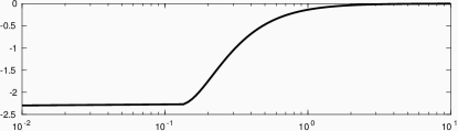
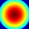
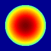
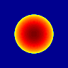
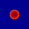
input $\mu$ $P=2.4$ $P=0.69$ $P=0.28$ $P=0.12$ $P=0.049$ $P=0.013$

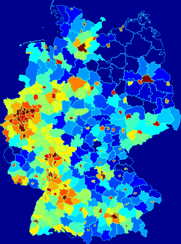
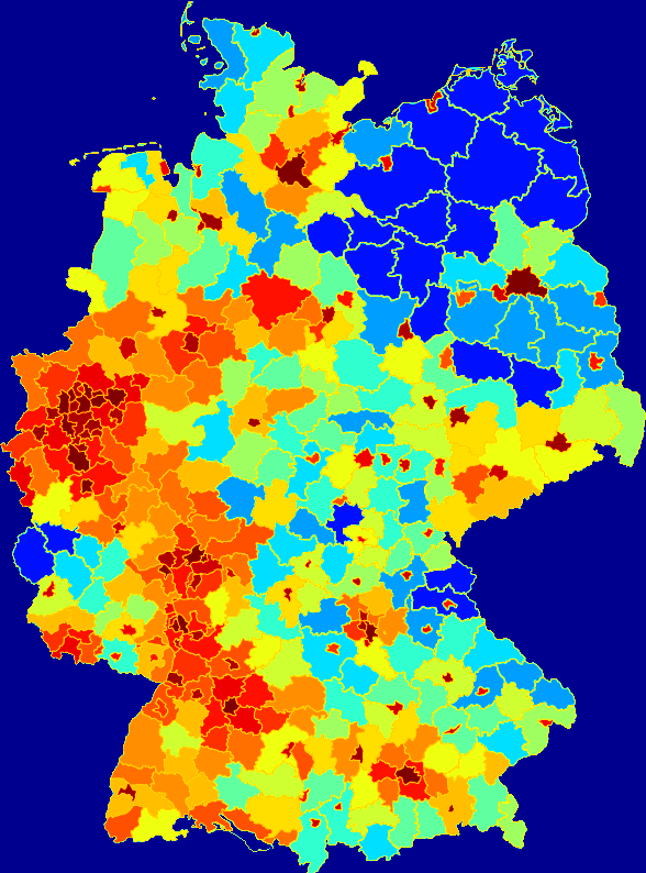
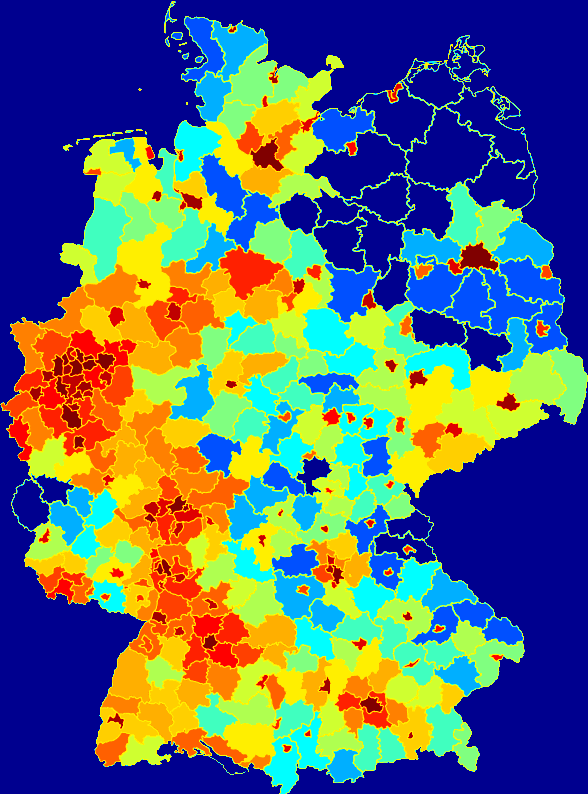
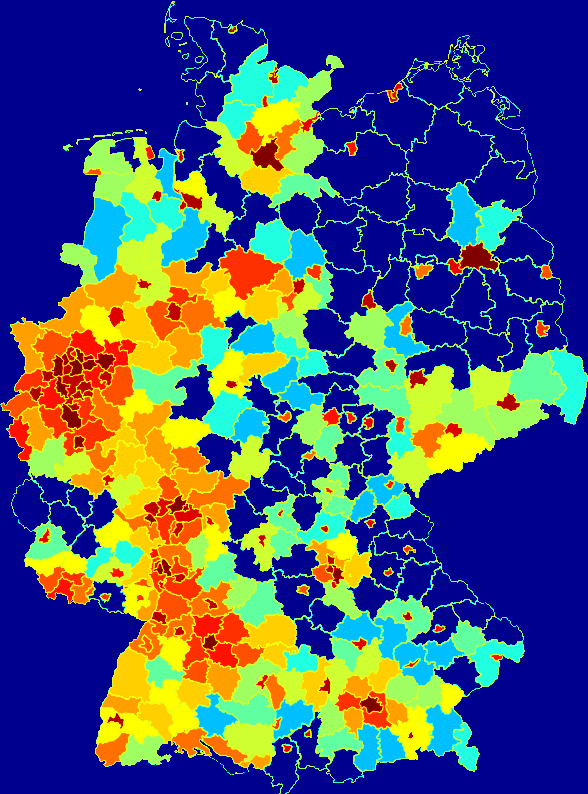
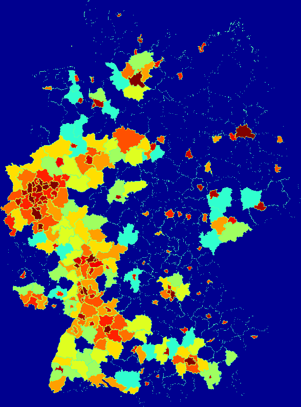
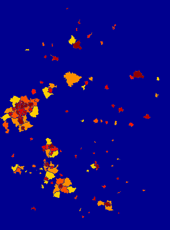
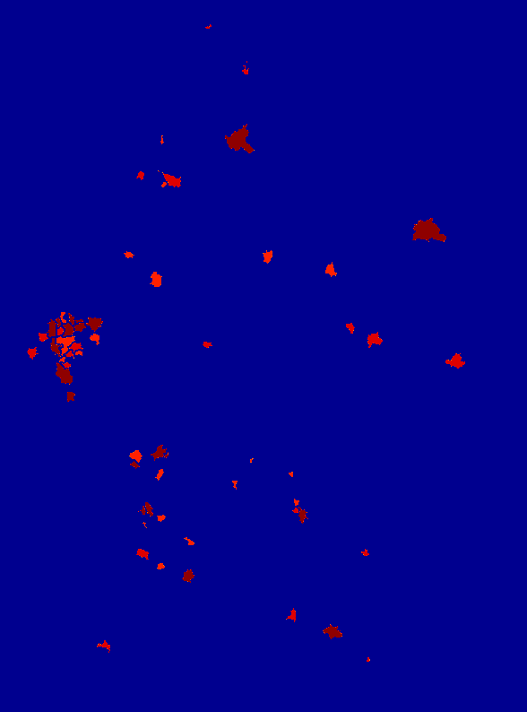
input $\mu$ $P=0.90$ $P=0.25$ $P=0.093$ $P=0.035$ $P=0.0075$ $P=0.0015$

Figure 11: Top row: $B^{\prime}$ from Lemma 4.11 for Wasserstein–Fisher–Rao transport. Middle and bottom row: input distribution $\mu$ (a Gaussian and same data as in Fig. 7) as well as asymptotically optimal point densities $D$ for different values of $P=\lim_{M\to\infty}\varepsilon_{M}^{2}M$ (colour-coding from blue for $0$ to red for maximum value).

References

- [1] L. Ambrosio, N. Fusco, and D. Pallara. Functions of Bounded Variation and Free Discontinuity Problems. Oxford University Press, 2000.
- [2] F. Aurenhammer, F. Hoffmann, and B. Aronov. Minkowski-type theorems and least-squares clustering. Algorithmica, 20(1):61–76, 1998.
- [3] F. Aurenhammer, R. Klein, and D.-T. Lee. Voronoi diagrams and Delaunay triangulations. World Scientific Publishing Company, 2013.
- [4] E. S. Barnes and N. J. A. Sloane. The optimal lattice quantizer in three dimensions. SIAM J. Algebraic Discrete Methods, 4(1):30–41, 1983.
- [5] H. H. Bauschke and P. L. Combettes. Convex Analysis and Monotone Operator Theory in Hilbert Spaces. Springer, 2011.
- [6] B. Bollobás and N. Stern. The optimal structure of market areas. J. Econ. Theory, 4(2):174–179, 1972.
- [7] G. Bouchitté, C. Jimenez, and R. Mahadevan. Asymptotic analysis of a class of optimal location problems. J. Math. Pures Appl., 95(4):382–419, 2011.
- [8] D. P. Bourne, M. A. Peletier, and F. Theil. Optimality of the triangular lattice for a particle system with Wasserstein interaction. Commun. Math. Phys., 329(1):117–140, 2014.
- [9] D. P. Bourne and S. M. Roper. Centroidal power diagrams, Lloyd’s algorithm, and applications to optimal location problems. SIAM J. Numer. Anal., 53(6):2545–2569, 2015.
- [10] D. Bourne, M. Peletier, and S. Roper. Hexagonal patterns in a simplified model for block copolymers. SIAM J. Appl. Math., 74(5):1315––1337, 2014.
- [11] G. Buttazzo and F. Santambrogio. A mass transportation model for the optimal planning of an urban region. SIAM Rev., 51(3):593–610, 2009.
- [12] E. Caglioti, F. Golse, and M. Iacobelli. A gradient flow approach to quantization of measures. Math. Models Methods Appl. Sci., 25(10):1845–1885, 2015.
- [13] L. Chizat, G. Peyré, B. Schmitzer, and F.-X. Vialard. Unbalanced optimal transport: Dynamic and Kantorovich formulations. To appear in J. Funct. Anal., arXiv:1508.05216, 2015.
- [14] L. Chizat, G. Peyré, B. Schmitzer, and F.-X. Vialard. An interpolating distance between optimal transport and Fisher–Rao metrics. Found. Comp. Math., 18(1):1–44, 2018.
- [15] Q. Du, V. Faber, and M. Gunzburger. Centroidal Voronoi tessellations: Applications and algorithms. SIAM Rev., 41(4):637–676, 1999.
- [16] Q. Du, M. Gunzburger, L. Ju, and X. Wang. Centroidal Voronoi tessellation algorithms for image compression, segmentation, and multichannel restoration. J. Math. Imaging Vis, 24(2):177–194, 2006.
- [17] Q. Du and D. S. Wang. The optimal centroidal Voronoi tessellations and the Gersho’s conjecture in the three-dimensional space. Comput. Math. Appl., 49(9-10):1355–1373, 2005.
- [18] M. Emelianenko, L. Ju, and A. Rand. Nondegeneracy and weak global convergence of the Lloyd algorithm in . SIAM J. Numer. Anal., 46(3):1423–1441, 2008.
- [19] A. Figalli. The optimal partial transport problem. Arch. Ration. Mech. Anal., 195(2):533–560, 2010.
- [20] A. Galichon. Optimal Transport Methods in Economics. Princeton University Press, 2016.
- [21] W. Gangbo and R. J. McCann. The geometry of optimal transportation. Acta Math., 177(2):113–161, 1996.
- [22] A. Gersho. Asymptotically optimal block quantization. IEEE Trans. on Inform. Theory, 25(4):373–380, 1979.
- [23] A. Gersho and R. Gray. Vector Quantization and Signal Compression. Springer, 1992.
- [24] S. Graf and H. Luschgy. Foundations of Quantization for Probability Distributions. Springer, 2000.
- [25] P. M. Gruber. A short analytic proof of Fejes Tóth’s theorem on sums of moments. Aequationes Math., 58(3):291–295, 1999.
- [26] P. M. Gruber. Optimum quantization and its applications. Adv. Math., 186(2):456–497, 2004.
- [27] P. M. Gruber. Convex and Discrete Geometry. Springer, 2007.
- [28] J. Kitagawa, Q. Mérigot, and B. Thibert. Convergence of a Newton algorithm for semi-discrete optimal transport. To appear in J. Eur. Math. Soc, arXiv:1603.05579, 2016.
- [29] B. Kloeckner. Approximation by finitely supported measures. ESAIM Control Optim. Calc. Var., 18(2):343–359, 2012.
- [30] S. Kondratyev, L. Monsaingeon, and D. Vorotnikov. A new optimal transport distance on the space of finite Radon measures. Adv. Differential Equ., 21(11-12):1117–1164, 2016.
- [31] L. Larsson, R. Choksi, and J. C. Nave. Geometric self-assembly of rigid shapes: A simple Voronoi approach. SIAM J. Appl. Math., 76(3):1101–1125, 2016.
- [32] B. Lévy. A numerical algorithm for L2 semi-discrete optimal transport in 3D. ESAIM Math. Model. Numer. Anal., 49(6):1693–1715, 2015.
- [33] M. Liero, A. Mielke, and G. Savaré. Optimal entropy-transport problems and a new Hellinger–Kantorovich distance between positive measures. Invent. Math., 211(3):969–1117, 2018.
- [34] S. P. Lloyd. Least squares quantization in PCM. IEEE Trans. on Inform. Theory, 28(2):129–137, 1982.
- [35] X. Y. Lu and D. Slepčev. Properties of minimizers of average-distance problem via discrete approximation of measures. SIAM J. Math. Anal., 45(5):3114–3131, 2013.
- [36] J. B. MacQueen. Some methods for classification and analysis of multivariate observations. In Proceedings of 5th Berkeley Symposium on Mathematical Statistics and Probability, 1, pages 281–297. University of California Press, 1967.
- [37] Q. Mérigot. A multiscale approach to optimal transport. Comput. Graph. Forum, 30(5):1583–1592, 2011.
- [38] F. Morgan and R. Bolton. Hexagonal economic regions solve the location problem. Am. Math. Monthly, 109(2):165–172, 2002.
- [39] S. Mosconi and P. Tilli. –convergence for the irrigation problem. J. of Conv. Anal., 12(1):145–158, 2005.
- [40] D. Newman. The hexagon theorem. IEEE Trans. on Inform. Theory, 28(2):137–139, 1982.
- [41] G. Pagès, H. Pham, and J. Printems. Optimal quantization methods and applications to numerical problems in finance. In S. Rachev, editor, Handbook of Computational and Numerical Methods in Finance. Birkhäuser, 2004.
- [42] G. Peyré and M. Cuturi. Computational optimal transport. arXiv:1803.00567, 2015.
- [43] R. T. Rockafellar. Convex Analysis. Princeton University Press, 2nd edition, 1972.
- [44] M. Sabin and R. Gray. Global convergence and empirical consistency of the generalized Lloyd algorithm. IEEE Trans. on Inform. Theory, 32(2):148–155, 1986.
- [45] F. Santambrogio. Optimal Transport for Applied Mathematicians. Birkhäuser, 2015.
- [46] B. Schmitzer and B. Wirth. Dynamic models of Wasserstein-1-type unbalanced transport. To appear in ESAIM Control Optim. Calc. Var., arXiv:1705.04535, 2017.
- [47] M. Thorpe, F. Theil, A. M. Johansen, and N. Cade. Convergence of the -means minimization problem using -convergence. SIAM J. Appl. Math., 75(6):2444–2474, 2015.
- [48] G. F. Tóth. A stability criterion to the moment theorem. Studia Sci. Math. Hungar., 38(1):209–224, 2001.
- [49] L. F. Tóth. Lagerungen in der Ebene auf der Kugel und im Raum. Springer, 1972.
- [50] C. Villani. Optimal Transport: Old and New. Springer, 2009.
- [51] P. L. Zador. Asymptotic quantization error of continuous signals and the quantization dimension. IEEE Trans. Inform. Theory, 28(2):139–149, 1982.
- [52] C. Zhu, R. H. Byrd, P. Lu, and J. Nocedal. Algorithm 778: L-BFGS-B: Fortran subroutines for large-scale bound-constrained optimization. ACM Trans. Math. Softw., 23(4):550–560, 1997.