Analytic slowing-down distributions as modified by turbulent transport

Abstract

The effect of electrostatic microturbulence on fast particles rapidly decreases at high energy, but can be significant at moderate energy. Previous studies found that, in addition to changes in the energetic particle density, this results in nontrivial changes to the equilibrium velocity distribution. These effects have implications for plasma heating and the stability of Alfvén eigenmodes, but make multiscale simulations much more difficult without further approximations. Here, several related analytic model distribution functions are derived from first principles with reasonable approximations. A single dimensionless parameter characterizes the relative strength of turbulence relative to collisions, and this parameter appears as an exponent in the model distribution functions. Even the most simple of these models reproduces key features of the numerical phase-space transport solution and provides a useful a priori heuristic for determining how strong the effect of turbulence is on the redistribution of energetic particles in toroidal plasmas.

1 Introduction

Energetic particles, such as those utilized to heat plasma in magnetic confinement experiments, are subject to being redistributed by turbulent transport. The net flux of these non-Maxwellian energetic particles between flux surfaces is a strong function of energy (Hauff et al., 2009), and this causes the lower-energy (though still not thermalized) part of the velocity distribution to be “carved out”, sometimes leaving a bump-on-tail feature (Wilkie et al., 2016). Here, a simplified model which describes this effect is introduced, with a particular focus on alpha particles produced by the deuterium-tritium (DT) fusion reaction. It is a generalization of the analytic slowing-down distribution of Gaffey (Gaffey, 1976; Helander & Sigmar, 2002) (which will repeatedly be referred to as the “classical” slowing-down distribution) that includes an additional term mimicking the velocity dependence of microturbulent transport. An analytic distribution was also previously derived by Anderson et al. (1991) and Sigmar et al. (1993), wherein anomalous transport was treated with a constant diffusion coefficient, rather than one with velocity dependence.

Alpha particles are born isotropically from reacting deuterium and tritium nuclei at an energy of $E_{\alpha}=m_{\alpha}v_{\alpha}^{2}/2=3.52\,\mathrm{MeV}$. Plasma heating is caused by the friction of these particles against the bulk ions/electrons (which have characteristic thermal speeds $v_{ti/e}=\sqrt{2T_{i/e}/m_{i/e}}$, respectively). As they slow down and their magnetic orbits become smaller, alpha particles become more and more susceptible to ion-scale microturbulence. As they transport outward, they continue slowing down on outer flux surfaces. This, combined with the fact that fewer alpha particles are produced near the cooler edge of the plasma, means that the alpha particle energy leaving the plasma will be relatively be small (Kurki-Suonio et al., 2011). Even so, alpha particles will be redistributed radially, changing the global heating profile. Alphas then eventually become thermalized in equilibrium with the bulk ions, creating a population of helium “ash” with density $n_{\mathrm{ash}}>n_{\alpha}$ and temperature $T_{\mathrm{ash}}=T_{i}$. This population can then be treated as a Maxwellian impurity.

All of the aforementioned effects are captured by the kinetic transport equation from the low-collisionality ordering of gyrokinetics for the equilibrium distribution $f_{\alpha}$:

$$\frac{\partial f_{\alpha}}{\partial t}- \frac{1}{V^{\prime}}\frac{\partial}{\partial r}\left(V^{\prime}D_{rr}\frac{\partial f_{\alpha}}{\partial r}+V^{\prime}D_{rv}\frac{\partial f_{\alpha}}{\partial v}\right)-\frac{1}{v^{2}}\frac{\partial}{\partial v}\left(v^{2}D_{vr}\frac{\partial f_{\alpha}}{\partial r}+v^{2}D_{vv}\frac{\partial f_{\alpha}}{\partial v}\right)$$

$$=C\left[f_{\alpha}\right]+S_{\alpha}.$$ (1)

The collision operator $C$ includes collisions of trace particles against the Maxwellian bulk, and $S_{\alpha}(r,v)$ is the source of alpha particles from fusion reactions. Flux surfaces are labelled by the radial coordinate $r$, defined as the surface half-width at the height of the magnetic axis, and enclose a volume $V(r)$, and primes denote differentiation with respect to radius. The radius of the last closed flux surface is the plasma minor radius $a$. The various turbulent diffusion coefficients $D_{xx}$ are functions of radius and speed $v$, and these can be calculated from nonlinear gyrokinetic simulations. Equation (1) is valid for either trace impurities or for energetic particles (Wilkie et al., 2018). Both of these conditions are typically satisfied for alpha particles (Wilkie et al., 2015).

The main body of this work derives (Section 2), benchmarks, and discusses (Section 3) a particularly simple analytic distribution using a local loss term that models the approximate effect of energy-dependent transport. The approximate velocity dependence used is derived from first principles in Appendix A. Appendix B relaxes the isotropic approximation and leads to a velocity dependence with the same energy scaling, but a different pitch-angle scaling than Hauff et al. (2009). An analytic model distribution with pitch angle dependence is thereby also derived in Appendix B. Appendix C relaxes the local-sink approximation to solve analytically for the radial transport in a plasma that is uniform except for the energetic particle source. These generalizations are combined to obtain an analytic distribution in 3-dimensional phase space $f_{SD,3D}\left(r,v,\xi\right)$ in Eq. (32).

2 Model distribution function

An approximate local solution to Eq. (1) will be found after a series of assumptions. In this section, it will be assumed that the energetic particles are isotropic in velocity space, but this is relaxed in the more general treatment of Appendix B. Also, in the limit where $v_{ti}\ll v\ll v_{te}$, the collision operator acting on an isotropic alpha distribution reduces to the simplified form $C\left[f_{\alpha}\right]\approx\tau_{s}^{-1}v^{-2}\left(\partial/\partial v\right)\left(v_{c}^{3}+v^{3}\right)f_{\alpha}$, where the critical speed is defined as

$$v_{c}\equiv v_{te}\left(\frac{3\sqrt{\pi}}{4}\sum\limits_{i}\frac{n_{i}m_{e}}{n_{e}m_{i}}Z_{i}^{2}\right)^{1/3},$$ (2)

with the sum over all non-trace ionic species. The slowing-down time is:

$$\tau_{s}\equiv\frac{3}{16\sqrt{\pi}}\frac{m_{\alpha}m_{e}v_{te}^{3}}{Z_{\alpha}^{2}e^{4}n_{e}\ln\Lambda_{\alpha e}}.$$ (3)

Previous studies (Wilkie et al., 2017) found that the $D_{rv}$, $D_{vr}$ and $D_{vv}$ coefficients play a sub-dominant role compared to radial diffusion ($D_{rr}$) at high energy, so this will be the only transport term kept from Eq. (1). To see that this is justified, consider the two source terms in the gyrokinetic equation: $\omega e\left\langle\phi\right\rangle_{\mathbf{R}}\partial f_{\alpha}/\partial E$ and $(c/B)k_{y}\left\langle\phi\right\rangle_{\mathbf{R}}\partial f_{\alpha}/\partial r$ for the case of ion-scale turbulence ($\omega\sim v_{ti}/a$ is the frequency, $k_{y}\sim\rho_{i}^{-1}$ is a perpendicular wave number, $\rho_{i}$ is the thermal ion Larmor radius, $E$ is energy, $B$ is the magnetic field magnitude, and $\left\langle\cdot\right\rangle_{\mathbf{R}}$ denotes the gyroaverage). The former term contributes to $D_{rv}$ and the latter to $D_{rr}$. Therefore, the latter will dominate when $T_{i}\partial f_{\alpha}/\partial E\ll a\partial f_{\alpha}/\partial r$, as is the case for energetic particles. Similar arguments apply to $D_{vr}$ and $D_{vv}$ when comparing their definitions to $D_{rr}$ and $D_{rv}$ (Wilkie et al., 2016). See Appendix A for more details.

An analytic model is derived in Appendix C which includes the global radial diffusion operator, but includes other generous assumptions about the radial plasma profile. Here, a local approximation will be made for the radial diffusion term, where the radial derivatives are parametrized by a length scale such that:

$$\frac{1}{V^{\prime}}\frac{\partial}{\partial r}\left[V^{\prime}D_{rr}\frac{\partial f_{\alpha}}{\partial r}\right]=-\frac{D}{L_{\alpha}^{2}}f_{\alpha}.$$ (4)

This is done to capture the approximate effect of transport on the local velocity distribution without needing to solve the radial transport equation as was done in Wilkie et al. (2016). In this framework, transport acts as a velocity-dependent sink of alpha particles. In reality, transported particles move to other flux surfaces, where they continue to slow down. Therefore, this approximation represents a “worst-case scenario”. This excludes cases where the energetic particle density might be greater at some radii due to transport from inner flux surfaces. In such cases, a local model is inadequate and full radial transport solution of Eq. (1) is required (Wilkie et al., 2016).

Since one does not have the luxury of the full radial and velocity dependence of $f_{\alpha}$, an a priori proxy is desired for the purposes of defining $L_{\alpha}$. For the classical slowing-down distribution, $n_{\alpha}\propto S_{0}$, so the source is chosen to represent the radial derivative of the energetic particle distribution so that $\partial f_{\alpha}/\partial r\approx-f_{\alpha}/L_{\alpha}$. This defines the radial scale length:

$$L_{\alpha}^{-2}\equiv-\mathrm{max}\left[\frac{S_{0}^{\prime\prime}}{S_{0}}+\frac{S_{0}^{\prime}}{S_{0}}\left(\frac{D_{\alpha}^{\prime}}{D_{\alpha}}+\frac{V^{\prime}}{V}\right),0\right],$$ (5)

where $D_{\alpha}=D_{rr}\left(v=v_{\alpha}\right)$ is typically small, less than about $0.01\mathrm{m}^{2}/\mathrm{s}$. This form of $L_{\alpha}$ is kept in the main body of this work for generality, but it does have the drawback of choosing a relevant energy to represent the radial distribution of energetic particles. For an analytic model that relaxes this assumption, see Appendix C. The neoclassical diffusion of slowing-down alphas due to collisional pitch-angle scattering (Catto, 1987) is expected to even smaller than turbulent transport, though this may be enhanced by a lack of perfect toroidal symmetry near the plasma edge (Kurki-Suonio et al., 2011).

The model energy dependence of the diffusion coefficient used for this model is borrowed from Hauff et al. (2009):

$$D_{rr}=D_{\alpha}\frac{v_{\alpha}^{3}}{v^{3}}.$$ (6)

See Appendix A for details on how this scaling is found. In Appendix B, it is shown that this is good approximation to the more general case where the pitch-angle dependence of $D_{rr}$ is taken into account. This is because the range of pitch angles for which $D_{rr}$ departs from this $v^{-3}$ scaling is very narrow (Pueschel et al., 2012).

One benefit of the locality approximation is that it reduces the effect of transport to a single dimensionless parameter, which shall be defined as:

$$b\equiv\frac{D_{\alpha}\tau_{s}}{L_{\alpha}^{2}}\frac{v_{\alpha}^{3}}{v_{c}^{3}}.$$ (7)

The appearance of the factor $v_{\alpha}^{3}/v_{c}^{3}$ is curious, but is motivated by the solution that follows. This dimensionless parameter can be simplified further by scaling the diffusion coefficient similarly to Pueschel et al. (2012). There, the diffusion coefficient at thermal energies was deemed proportional to the effective thermal diffusivity $\chi_{\mathrm{eff}}$. If it is supposed that $D_{rr}\left(v=v_{c}\right)\approx\chi_{\mathrm{eff}}$, then one can approximate $b\approx\chi_{\mathrm{eff}}\tau_{s}/L_{\alpha}^{2}$.

With the aforementioned approximations, Eq. (1) reduces to:

$$\frac{b}{\tau_{s}}\frac{v_{c}^{3}}{v^{3}}f_{\alpha}=\frac{1}{\tau_{s}}\frac{1}{v^{2}}\frac{\partial}{\partial v}\left[\left(v_{c}^{3}+v^{3}\right)f_{\alpha}\right]+S_{\alpha}$$ (8)

in steady-state. In this model, the transport term diverges as $v\rightarrow 0$. More realistically, one could define a cutoff speed below which the diffusion coefficient is constant – this also results in an analytic solution. However, due to the other approximations made, Eq. (8) is invalid at low energy, where the distribution is dominated by thermalized helium ash. Therefore, a bare $D_{rr}\propto v^{-3}$ scaling, without an ad-hoc cutoff, is used without significant reservation. This is done with the knowledge that, like the classical slowing-down distribution, it is not valid for $v\lesssim v_{ti}$. Unfortunately, this precludes a useful analogous generalization for heated minority ions (Pusztai et al., 2016) since it is much more sensitive to the diffusion coefficient at low energy, for which a reduced model has yet to be developed. However, the generalization to injected auxiliary fast ions (e.g. neutral beams) is straightforward, even if their injection energy is not as high as for alpha particles.

The solution to Eq. (8) is:

$$f_{\alpha}=\frac{\tau_{s}}{v_{c}^{3}+v^{3}}\left(\frac{v^{3}}{v^{3}+v_{c}^{3}}\right)^{b/3}\int_{\infty}^{v}S_{\alpha}\left(v^{\prime}\right)\left(\frac{v^{\prime 3}}{v^{\prime 3}+v_{c}^{3}}\right)^{-b/3}\,\mathrm{d}v^{\prime}.$$ (9)

Now the choice of including $v_{\alpha}^{3}/v_{c}^{3}$ in the definition of $b$, Eq. (7), becomes clear: this factor appears in the exponent of this distribution, and is thereby important in quantifying the effect of turbulence on the energetic particle distribution. Even for fusion-produced alpha particles, the source $S_{\alpha}$ has a significant spread in energy proportional to the geometric mean of the fuel temperature and the alpha particle birth energy (Brysk, 1973). However, in order to obtain an analytic solution, it will be convenient to use a mono-energetic source such that $S_{\alpha}\approx\left(S_{0}/4\pi v_{\alpha}^{2}\right)\delta\left(v-v_{\alpha}\right)$. The following analytic model distribution is thereby found:

$$F_{SD,\mathrm{mod}}=\frac{S_{0}\tau_{s}}{4\pi}\frac{1}{v_{c}^{3}+v^{3}}\left(\frac{v^{3}}{v_{\alpha}^{3}}\frac{v_{\alpha}^{3}+v_{c}^{3}}{v^{3}+v_{c}^{3}}\right)^{b/3}H\left(v_{\alpha}-v\right),$$ (10)

where $H$ is the Heaviside step function. Equation (10) reduces to the classical slowing-down distribution when transport is negligible: $b=0$. This is a generalization of the analytic distribution found by Sigmar et al. (1993) to the case of energy-dependent diffusion as given by Eq. (6). Representative examples of this distribution at different values of $b$ are shown in Fig. 1.

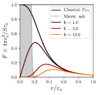
Figure 1: Comparing the classical Gaffey slowing-down distribution with the analytic transport-modified version – Eq. (10) – for different values of $b$. Lighter shades corresponding to higher relative turbulence intensity. The shaded area represents the Maxwellian ash population for $n_{\mathrm{ash}}=10n_{\alpha}$ and $T_{\mathrm{ash}}=E_{\alpha}/350$. For these cases, $v_{c}=0.3v_{\alpha}$.

3 Benchmarking and discussion

There are several curious features of the distribution described by Eq. (10) which are nevertheless backed up by numerical simulations and physical insight.

Firstly, $F_{SD,\mathrm{mod}}(v)$ has a local maximum at $v_{*}=v_{\alpha}\left(D_{\alpha}\tau_{s}/3L_{\alpha}^{2}\right)^{1/3}$. Therefore, the distribution exhibits a “bump-on-tail” similar to what was previously observed (Wilkie et al., 2016, 2017). In order for this inversion to be observable, this maximum must be well separated from the helium ash population. Therefore, a bump-on-tail caused by turbulent transport is possible only if:

$$D_{\alpha}\gg\frac{3L_{\alpha}^{2}}{\tau_{s}}\left(\frac{v_{t,\mathrm{ash}}}{v_{\alpha}}\right)^{3}.$$ (11)

Using $T_{i}\sim 10\mathrm{keV}$, $\tau_{s}\sim 1\mathrm{s}$, and $L_{\alpha}\sim 0.4\mathrm{m}$, the presence of a bump requires $D_{\alpha}\gg 7\times 10^{-5}\mathrm{m}^{2}/\mathrm{s}$. Estimates of $D_{\alpha}$ from the literature range from about $6\times 10^{-4}$ to $2\times 10^{-2}\mathrm{m}^{2}/\mathrm{s}$ using gyrokinetic simulations (Hauff et al., 2009; Zhang et al., 2010; Pueschel et al., 2012; Wilkie et al., 2015), making this condition marginally- or well-satisfied depending on the scenario. The presence of a local maximum in velocity space has the potential to destabilize waves, such as Alfvén eigenmodes, via inverse Landau damping. A flattening or inversion in velocity space is destabilizing, but it accompanied by a flattening of the radial profile, which is stabilizing. Without a detailed analysis, it is not immediately clear what the net effect is.

Also, notice that, at the birth speed $v=v_{\alpha}$, there is no turbulent correction to the classical slowing-down distribution. No matter how strong the turbulence is, it will not affect newly-born alpha particles because it cannot possibly compete with a delta function at its peak. As the alpha particle slows down, it becomes doubly affected because it is further away in velocity space from the source in addition to turbulent transport becoming stronger. Since most of the electron heating occurs near the injection speed, this remains immune to turbulent transport of alphas. What might be affected is the heating of ions at lower energy.

The model distribution was benchmarked against a numerical solution of Eq. (1). The test case is an ITER-like ELMy H-mode DT scenario that is unstable to electrostatic ion-temperature gradient turbulence beyond $r=0.5a$. It can be found on the public tokamak profile database (Roach et al., 2008) as ITER scenario 10010100. In these simulations, the diffusion coefficient was calculated directly from first-principles gyrokinetic simulations (and thus did not diverge as $v\rightarrow 0$). Further, the full test-particle collision operator was used to capture physically consistent thermalization of helium ash. For more details about the transport of alpha particles in this case, see Wilkie et al. (2016).

The local distribution function at two different radii are shown in Fig. 2. Despite the generous assumptions built into the analytic model, it qualitatively captures the basic features of the numerical solution including: well-confined high-energy alphas, a depletion of the distribution at more moderate energies, and the bump-on-tail feature. At these radii ($r=0.5a$ and $0.6a)$, the values of $b$ were found to be 5.3 and 2.6, respectively.

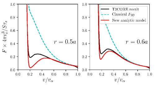
Figure 2: Comparing the local velocity distribution function of alpha particles for two different radii of the ITER-like scenario of (Wilkie et al., 2016). Shown are the Gaffey slowing-down distribution (cyan dashed line), Eq. (10) (red line), and a numerical phase-space transport solution (black line). Each of the analytic distributions are shown with a population of Maxwellian ash added, equal to the ash density calculated with t3core.

The alpha particle density as a function of radius for the test case is shown in Fig. 3. There, the analytic solution is compared to the numerical transport solution and to the slowing-down distribution without radial transport. Even when the classical density differs from the numerical one due to transport, Eq. (10) captures this difference fairly well. This motivates using the model as a heuristic to answer the question: “can one expect significant energetic particle transport from microturbulence?” An affirmative answer indicates that further study is warranted, but if $b<1$, the classical slowing-down distribution is reasonably accurate.

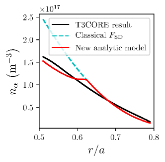
Figure 3: Comparing the radial density profile of energetic alpha particles as predicted by the Gaffey slowing-down distribution (cyan dashed line), Eq. (10) (red line), and a numerical phase-space transport solution (black line).

4 Conclusion

This work introduced and briefly discussed a simplified model for slowing-down alpha particles in the presence of microturbulence. Although heuristic, this model distribution captures the approximate effect of turbulence through a single dimensionless parameter, which has a stronger impact than one might expect when the birth speed $v_{\alpha}$ significantly exceeds the critical speed $v_{c}$. When relaxing several assumptions made for this simple model, more robust analytic distributions are found which maintain the same basic character of Eq. (10). Although more detailed simulations are generally required to robustly predict the impact of microturbulence on plasma heating, Alfvén eigenmode drive, and other effects mediated by energetic particles, this model provides physical insight into the expected effect of microturbulence on these phenomena.

The author would like to thank I. Pusztai, I. Abel, and T. Fülöp for helpful comments in preparing this manuscript. The author was supported by the EUROfusion Researcher Grant AWP18-ERG-VR. The views and opinions expressed herein do not necessarily reflect those of the European Commission.

Appendix A Energy scaling of the diffusion coefficient

In this section, the fluctuating distribution of energetic particles is analyzed to motivate the energy scaling of the diffusion coefficient used in this work (Hauff et al., 2009). Only electrostatic fluctuations will be considered here. After finding a solution to the gyrokinetic equation in the high-energy limit as was done in Wilkie et al. (2018), the radial flux is averaged over the spatial and temporal scale of the fluctuations. The diffusion coefficient is what remains after factoring out $\partial F_{0\alpha}/\partial r$. In the mean time, it will become apparent why radial diffusion is dominant over the other turbulent terms of Eq. (1) in this limit.

The collisionless gyrokinetic equation for non-Maxwellian fast particles is (Frieman & Chen, 1982; Wilkie, 2015; Abel et al., 2018):

$$\frac{\partial h_{\alpha}}{\partial t}+v_{\|}\mathbf{b}\cdot\nabla h_{\alpha}+\left(\mathbf{v}_{D}+\mathbf{v}_{\phi}\right)\cdot\nabla h_{\alpha}=Z_{\alpha}e\frac{\partial F_{0\alpha}}{\partial\mathcal{E}}\frac{\partial\left\langle\phi\right\rangle_{\mathbf{R}}}{\partial t}-\mathbf{v}_{\phi}\cdot\nabla F_{0\alpha},$$ (12)

where it is expressed in the coordinates $\mathcal{E}=Z_{\alpha}e\phi+m_{\alpha}v^{2}/2$, and $\mu$, which is the exactly conserved magnetic moment. With this definition, $\partial F_{0\alpha}/\partial\mu$ does not appear in Eq. (12). It does appear, along with the adiabatic contribution, in the equations that determine the fluctuating fields, which will not be used here. The distribution is decomposed into an equilibrium part $F_{0\alpha}$ and a fluctuating part $h_{\alpha}$ such that $f_{\alpha}=F_{0\alpha}+h_{\alpha}$. The magnetic field is given in the Clebsch representation as $\mathbf{B}=B\mathbf{b}=\nabla\alpha\times\nabla\psi$, where $\psi$ is the poloidal flux in the flux surface that it labels and $\alpha$ (not to be confused with the subscript denoting energetic particles) labels the magnetic field line within said flux surface. The velocity parallel to the magnetic field is $v_{\|}=\sigma_{\|}\sqrt{\left(2/m_{\alpha}\right)\left(\mathcal{E}-\mu B\left(\theta\right)\right)}$ and $\theta$ is the ballooning-extended poloidal angle, used as a coordinate along the field line. The fluctuating static potential is $\phi$. The gyroaverage at constant gyrocenter $\mathbf{R}$ is denoted $\left\langle\right\rangle_{\mathbf{R}}$, and the spatial gradients in Eq. (12) are taken with respect to $\mathbf{R}$. The drift associated with the fluctuating fields is given by $\mathbf{v}_{\phi}\equiv\left(c/B\right)\mathbf{b}\times\nabla\left\langle\phi\right\rangle_{\mathbf{R}}$, and $\mathbf{v}_{D}$ is the magnetic drift due to the curvature and gradient in $\mathbf{B}$.

Consider that, in ion-scale turbulence, the bulk ions set the spatial and temporal scales for the variation of $\phi$ and $h_{\alpha}$. In the limit where $v_{t\alpha}\gg v_{ti}$, the magnetic drift, parallel streaming, and equilibrium gradient are the largest terms in Eq. (12). The “nonlinear” $\mathbf{v}_{\phi}$ term is thereby small. It is convenient and conventional to express the fluctuating quantities in an eikonal representation so that $\phi=\hat{\phi}\left(\theta\right)\exp\left[iS\left(\psi,\alpha\right)\right]$, where $S$ contains the small-scale variation perpendicular to the magnetic field and $\hat{\phi}$ is the relatively long-scale parallel variation (Antonsen & Lane, 1980). In this representation, the energetic limit of Eq. (12) reduces to:

$$v_{\|}\mathbf{b}\cdot\nabla\theta\frac{\partial\hat{h}_{\alpha}}{\partial\theta}+i\mathbf{v}_{D}\cdot\nabla S\hat{h}_{\alpha}=ic\frac{\partial S}{\partial\alpha}\frac{\partial F_{0\alpha}}{\partial\psi}\hat{\phi},$$ (13)

Even near the source, where $\partial F_{0\alpha}/\partial\mathcal{E}\sim F_{0\alpha}/T_{i}$, the first term on the right hand side of Eq. (12) (which ultimately contributes to $D_{rv}$) is smaller than the first term (which leads to $D_{rr}$) on the right hand side of Eq. (13) by virtue of the large spatial gradients in the source of energetic particles (and therefore in $F_{0\alpha}$ itself). In any case, at energies this high, collisions acting on the equilibrium dominate both $D_{rr}$ and $D_{rv}$. Away from the source, where turbulence is observed to have an effect, $\partial F_{0\alpha}/\partial\mathcal{E}\sim F_{0\alpha}/E_{\alpha}$, and this term is smaller still. Similar arguments apply to the turbulent heating terms ($D_{vr}$ and $D_{vv}$), only moreso. Furthermore, if the $\partial\left\langle\phi\right\rangle_{\mathbf{R}}/\partial t$ term were kept, its contribution to the time-averaged radial flux vanishes in the energetic (thereby, linear) limit because $\int\phi\dot{\phi}\,\mathrm{d}t=0$ in steady-state by definition. It is for these reasons that radial diffusion is dominant over other terms in Eq. (1).

In finding an integrating factor to solve Eq. (13), it will be convenient to define:

$$z\left(\theta\right)\equiv\int^{\theta}_{\theta_{0}}\frac{\omega_{D}^{\prime}\,\mathrm{d}\theta^{\prime}}{v_{\parallel}^{\prime}\left(\mathbf{b}\cdot\nabla\theta\right)^{\prime}},$$ (14)

where $\omega_{D}\equiv\mathbf{v}_{D}\cdot\nabla S$ and $\omega_{D}\left(\theta_{0}\right)=0$. Primes denote quantities taken at $\theta^{\prime}$ rather than $\theta$. A saddle point is located at $\theta_{0}$ such that $\left[\mathrm{d}z/\mathrm{d}\theta\right]_{\theta_{0}}=0$. With this definition, the solution to Eq. (13) is (Kim et al., 1993; Wilkie et al., 2018):

$$\hat{h}_{\alpha}\left(\theta\right)=ic\frac{\partial F_{0\alpha}}{\partial\psi}\frac{\partial S}{\partial\alpha}\int^{\theta}J_{0}\left(\frac{|\nabla S|v_{\perp}}{\Omega_{\alpha}\left(\theta^{\prime}\right)}\right)\phi\left(\theta^{\prime}\right)\exp\left[iz\left(\theta\right)-iz\left(\theta^{\prime}\right)\right]\frac{\mathrm{d}\theta^{\prime}\,}{v_{\parallel}^{\prime}\left(\mathbf{b}\cdot\nabla\theta\right)^{\prime}},$$ (15)

where $J_{0}$ is the zeroth-order Bessel function of the first kind and $\Omega_{\alpha}\equiv Z_{\alpha}eB/m_{\alpha}c$ is the gyrofrequency. The lower limit of integration in Eq. (15) is either $\pm\infty$ for passing particles depending on the sign of $v_{\|}$, or $\pm\theta_{b}$ if the particles are trapped. Expanding $z$ in a Taylor series about $\theta_{0}$ leaves a Gaussian which is integrated over the contour of steepest descent, taking advantage of the fact that $z\gg 1$ to obtain:

$$\hat{h}_{\alpha}\left(\theta\right)\approx ic\frac{\partial F_{0\alpha}}{\partial\psi}\frac{\partial S}{\partial\alpha}e^{i\left(z_{0}-z\right)}J_{0}\left(\frac{|\nabla S|v_{\perp}}{\Omega_{\alpha}\left(\theta_{0}\right)}\right)\frac{\phi\left(\theta_{0}\right)}{\left[v_{\parallel}\left(\mathbf{b}\cdot\nabla\theta\right)\right]_{0}}\sqrt{\frac{2\pi i}{\zeta_{0}}},$$ (16)

where $\left[\,\right]_{0}$ denotes quantities taken at $\theta_{0}$, and $\zeta_{0}$ is defined as:

$$\zeta_{0}\equiv\left[\frac{\mathrm{d}^{2}z}{\mathrm{d}\theta^{2}}\right]_{\theta_{0}}=\left[\frac{\mathrm{d}}{\mathrm{d}\theta}\frac{\omega_{D}}{v_{\|}\mathbf{b}\cdot\nabla\theta}\right]_{\theta_{0}}.$$ (17)

The approximate solution of Eq. (16) excludes deeply trapped particles; namely those that bounce at a poloidal location $|\theta_{b}|\lesssim|\theta_{0}|$.

The radial flux is kept as a function of velocity in the kinetic phase space transport equation, and is defined as:

$$\Gamma_{\alpha}\equiv\left\langle\sum\limits_{\sigma_{\|}}\int_{-\infty}^{\infty}h_{\alpha}\mathbf{v}_{\phi}\cdot\nabla r\,\mathrm{d}\theta\right\rangle_{\perp,t},$$ (18)

where $\left\langle\,\right\rangle_{\perp}$ is a perpendicular spatial average over the flux tube and a time average over the the fluctuation timescale (Abel et al., 2013). In performing the $\theta$ integral, apply the same large-$z$ approximation that led to Eq. (16). Also note that $h_{\alpha}$ is proportional to $\partial F_{0\alpha}/\partial\psi$, allowing one to write $\Gamma_{\alpha}=-D_{rr}\partial F_{0\alpha}/\partial r$ for $\psi=\psi\left(r\right)$. This gives:

$$D_{rr}\approx\left\langle 2\pi c^{2}\left(\frac{\mathrm{d}r}{\mathrm{d}\psi}\right)^{2}\left(\frac{\partial S}{\partial\alpha}\right)^{2}J_{0}^{2}\left(\frac{|\nabla S|v_{\perp}}{\Omega_{\alpha}\left(\theta_{0}\right)}\right)\frac{\left|\phi\left(\theta_{0}\right)\right|^{2}}{\left|\left(v_{\|}\mathbf{b}\cdot\nabla\theta\right)_{\theta_{0}}\left.\frac{\mathrm{d}}{\mathrm{d}\theta}\right|_{\theta_{0}}\frac{\omega_{D}}{v_{\|}\mathbf{b}\cdot\nabla\theta}\right|}\right\rangle_{\perp,t}.$$ (19)

The origin of the $v^{-3}$ scaling of Hauff et al. (2009) is now apparent by counting powers of $v$, noting that $J_{0}\left(x\gg 1\right)\sim x^{-1/2}$ and $\omega_{D}\propto v^{2}$. It was with this scaling that the isotropic slowing-down distribution function was found in Eq. (10).

Appendix B Pitch-angle dependence and anisotropic distribution

In this section, the pitch-angle dependence of the approximate diffusion coefficient in Eq. (19) is kept to obtain a slowing-down distribution that includes pitch-angle dependent transport. Thus an anisotropic equilibrium distribution for weakly collisional energetic particles is derived. Doing so will require making further assumptions about the turbulent spectrum that should have minimal impact at high energy. By using the value of the diffusion coefficient at $\xi=0$, it will be found that Eq. (10) remains an adequate approximation to the anisotropic distribution up to $|\xi|\approx 0.9$.

To facilitate calculating the perpendicular spatial average in Eq. (19), make the ansatz that the turbulent spectrum is on the ion Larmor radius scale and has the following form:

$$\left|\phi\left(\mathbf{k}_{\perp}\right)\right|^{2}=\left|\phi_{0}\right|^{2}_{\mathrm{max}}\delta\left(k_{x}\right)\frac{k_{y}^{2}}{k_{\mathrm{max}}^{2}}e^{-k_{y}^{2}/k_{\mathrm{max}}^{2}+1}$$ (20)

where $k_{y}\equiv a^{-1}\partial S/\partial\alpha$ and $k_{\mathrm{max}}\sim\rho_{i}^{-1}$ is the wavenumber at the peak of the turbulent spectrum. The exact form of the spectrum does not significantly impact the functional dependence of the result at high energy (especially when $D_{\alpha}$ is assumed given as it is here), but provides a meaningful cutoff that will prove necessary. Integrating over all $k_{y}$ smooths the oscillations in the Bessel function and $\omega_{D}\propto k_{y}\left(v_{\|}^{2}+v_{\perp}^{2}/2\right)$. Equation (19) is thereby well-approximated by:

$$D_{rr}\approx D_{\alpha}\frac{v_{\alpha}^{3}}{v^{3}}\frac{1}{1+\xi^{2}}\frac{1}{\sqrt{1-\xi^{2}}+\frac{v_{ti}}{v}\frac{1}{2\sqrt{\pi}k_{\mathrm{max}}\rho_{i}}},$$ (21)

where $D_{\alpha}$ is the diffusion coefficient at $\xi=0$ and $v=v_{\alpha}\gg v_{ti}$. The rightmost factor comes from the Padé approximation $\int_{0}^{\infty}k^{3}e^{-k^{2}}J_{0}^{2}\left(ak\right)\,\mathrm{d}k\approx\left(4\sqrt{\pi}a+2\right)^{-1}$. This approximate form contains all the velocity dependence of the diffusion coefficient, which is shown in Fig. 4. Equation (21) recovers the energy dependence of both electrostatic limits considered in Hauff et al. (2009), but avoids singularities in pitch angle. The pitch angle dependence in Eq. (21) is approximately constant except for a narrow region near $\xi=\pm 1$. There, the diffusion coefficient becomes large and the energy dependence changes to $v^{-2}$ (Pueschel et al., 2012). This represents the part of phase space where the energetic particle’s Larmor radius becomes comparable to $\rho_{i}$, despite its large energy, by virtue of its large pitch-angle. In this regime, the details of the turbulence do matter and the ansatz made in Eq. (20) becomes unreliable. In any case, one can nevertheless expect a significant increase in the diffusion coefficient when $v\approx|v_{\|}|$.

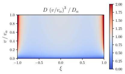
Figure 4: Velocity dependence of the diffusion coefficient, Eq. (21), as compared to the isotropic form, Eq. (6). Here, $v_{c}=0.3v_{\alpha}$ and $v_{ti}=0.15k_{\mathrm{max}}\rho_{i}v_{\alpha}$.

Consider the low-collisionality transport equation with pitch angle scattering included as well as the $\xi$ dependence of transport given by Eq. (21):

$$b\frac{v_{c}^{3}}{v^{3}} \left[\left(1+\xi^{2}\right)\left(\sqrt{1-\xi^{2}}+\frac{v_{ti}}{2v\sqrt{\pi}k_{\mathrm{max}}\rho_{i}}\right)\right]^{-1}f_{\alpha}$$ (22)

$$=\frac{1}{2}\frac{v_{ti}^{3}}{v^{3}}\frac{\partial}{\partial\xi}\left(1-\xi^{2}\right)\frac{\partial f_{\alpha}}{\partial\xi}+\frac{1}{v^{2}}\frac{\partial}{\partial v}\left[\left(v_{c}^{3}+v^{3}\right)f_{\alpha}\right]+\frac{S_{0}\tau_{s}}{4\pi v_{\alpha}^{2}}\delta\left(v-v_{\alpha}\right),$$

where the $v\gg v_{ti}$ limit was used for the deflection collision frequency on the Lorentz operator. Note that, unless $\partial\ln f_{\alpha}/\partial\xi\gtrsim\mathcal{O}\left(v_{c}^{3}/v_{ti}^{3}\right)$, the pitch-angle scattering term is small. In this case, a complicated, but analytic $f_{\alpha}$ can be found with the help of the integrating factor $\left(v_{c}^{3}+v^{3}\right)\exp\left(g\right)$, where

$$g\left(v,\xi\right)= \frac{-b}{\left(1+\xi^{2}\right)}\frac{\pi}{24\pi^{2}v_{c}^{3}\left(1-\xi\right)^{3/2}-3\sqrt{\pi}v_{ti}^{3}}\times$$ (23)

$$\left\{2\sqrt{3}v_{c}v_{ti}\left(2\sqrt{\pi}v_{c}\sqrt{1-\xi^{2}}-v_{ti}\right)\tan^{-1}\left(\frac{2v-v_{c}}{\sqrt{3}v_{c}}\right)\right.$$

$$+v_{c}v_{ti}\left(2\sqrt{\pi}v_{c}\sqrt{1-\xi^{2}}+v_{ti}\right)\ln\left[\frac{v^{2}-vv_{c}+v_{c}^{2}}{\left(v_{c}+v\right)^{2}}\right]$$

$$\left.-8\pi v_{c}^{3}\left(1-\xi^{2}\right)\ln\left[\frac{v_{c}^{3}+v^{3}}{\left(2\sqrt{\pi}v\sqrt{1-\xi^{2}}+v_{ti}\right)^{3}}\right]\right\}.$$

The approximate distribution function with the full pitch-angle dependence of Eq. (21) is therefore:

$$F_{SD,\mathrm{mod}}\left(v,\xi\right)=\frac{S_{0}\tau_{s}}{4\pi}\frac{1}{v_{c}^{3}+v^{3}}\exp\left[g\left(v_{\alpha},\xi\right)-g\left(v,\xi\right)\right]H\left(v_{\alpha}-v\right).$$ (24)

This distribution is shown for select parameters in Fig. 5, and the pitch angle dependence is shown in Fig. 6. With this form, the assumption of negligible pitch angle scattering breaks down in the region $|\xi|\gtrsim 0.99$, where pitch angle derivatives become sufficiently large compared to the distribution. Also in this region, the turbulent spectrum used to derive Eq. (24) becomes unreliable because the transport will depend on the details of the turbulence, which can only be found from direct simulation.

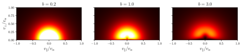
Figure 5: Pitch angle dependence of the generalized slowing-down distribution, Eq. (24), for several values of turbulent intensity (parametrized by $b$). Here, $v_{c}=0.3v_{\alpha}$ and $v_{ti}=0.15k_{\mathrm{max}}\rho_{i}v_{\alpha}$.

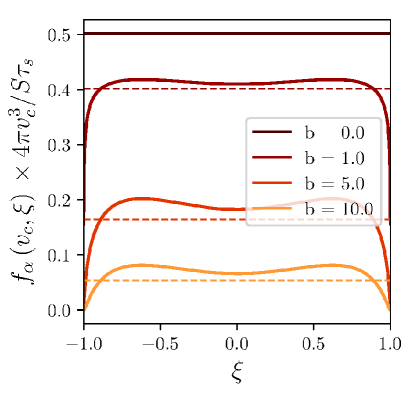
Figure 6: Pitch angle dependence of the generalized slowing-down distribution, Eq. (24), at $v=v_{c}=0.3v_{\alpha}$ and $v_{ti}=0.15k_{\mathrm{max}}\rho_{i}v_{\alpha}$. Dotted lines represent the value of the isotropic distribution, Eq. (10) using the diffusion coefficient at $\xi=0$.

Appendix C Global model

In this section, an analytic distribution with radial dependence is derived similarly, but more generally, than Anderson et al. (1991), which will aid in interpreting the length scale $L_{\alpha}$ more rigorously. This is possible for a fictitious radial profile in the large aspect ratio limit where $D_{rr}$, $\tau_{s}$, and $v_{c}$ are independent of radius, while the energetic particle source (which is typically more strongly peaked than the other parameters) retains full radial dependence. This establishes that the velocity dependence of the model maintains its general form even when consistently accounting for radial transport. Equation (32) provides a turbulence-modified analytic distribution with radial, energy, and pitch-angle dependence.

Expand the radial dependence of the source in a Fourier-Bessel series:

$$S_{\alpha}\left(r,v\right)=\sum\limits_{j=1}^{\infty}\frac{\sigma_{j}}{4\pi v_{\alpha}^{2}}J_{0}\left(a_{0,j}\frac{r}{a}\right)$$ (25)

where $\sigma_{1}$ is the velocity-integrated source at the magnetic axis and $a_{0,j}$ is the $j$th positive root of the zero-order Bessel function $J_{0}$. This diagonalizes the radial diffusion operator in the large-aspect ratio limit where $V^{\prime}\left(r\right)\propto r$. Expand $f_{\alpha}\left(r,v\right)=\sum f_{\alpha,j}\left(v\right)J_{0}\left(a_{0,j}r/a\right)$ and use the same approximations of Section 2 for radial diffusion, the collision operator, and source to obtain:

$$-\sum\limits_{j=1}^{\infty} f_{\alpha,j}\frac{1}{r}\frac{\partial}{\partial r}D_{\alpha}\frac{v_{\alpha}^{3}}{v^{3}}\frac{\partial}{\partial r}J_{0}\left(a_{0,j}\frac{r}{a}\right)+\frac{1}{\tau_{s}v^{2}}\frac{\partial}{\partial v}\left[\left(v_{c}^{3}+v^{3}\right)f_{\alpha,j}\right]J_{0}\left(a_{0,j}\frac{r}{a}\right)$$ (26)

$$=\sum\limits_{j=1}^{\infty}\frac{\sigma_{j}}{4\pi v_{\alpha}^{2}}\delta\left(v-v_{\alpha}\right)J_{0}\left(a_{0,j}\frac{r}{a}\right)=0.$$ (27)

After multiplying by $rJ_{0}\left(a_{0,k}r/a\right)$ and integrating from $r=0$ to $a$, the approximate equation for each Bessel mode $k$ is:

$$D_{\alpha}\frac{a_{0,k}^{2}}{a^{2}}\frac{v_{\alpha}^{3}}{v^{3}}f_{\alpha,k}-\frac{1}{\tau_{s}v^{2}}\frac{\partial}{\partial v}\left[\left(v_{c}^{3}+v^{3}\right)f_{\alpha,k}\right]+\frac{\sigma_{k}}{4\pi v_{\alpha}^{2}}\delta\left(v-v_{\alpha}\right).$$ (28)

This can be solved the same way as Eq. (8) to obtain:

$$f_{SD,r}\left(r,v\right)=\sum\limits_{j}\frac{\sigma_{j}\tau_{s}}{4\pi}\frac{1}{v_{c}^{3}+v^{3}}\left(\frac{v^{3}}{v_{\alpha}^{3}}\frac{v_{\alpha}^{3}+v_{c}^{3}}{v^{3}+v_{c}^{3}}\right)^{b_{j}/3}H\left(v_{\alpha}-v\right)J_{0}\left(a_{0,j}\frac{r}{a}\right)$$ (29)

where:

$$b_{j}\equiv\frac{D_{\alpha}\tau_{s}}{a^{2}}\frac{v_{\alpha}^{3}}{v_{c}^{3}}a_{0,j}^{2},$$ (30)

and

$$\sigma_{j}\equiv\frac{2\int_{0}^{a}S_{0}(r)J_{0}\left(a_{0,j}r/a\right)r\,\mathrm{d}r}{a^{2}J_{1}^{2}\left(a_{0,j}\right)}.$$ (31)

This is a radially global distribution approximately valid where the plasma profile (particularly, $D_{rr}$, $\tau_{s}$, and $v_{c}$) is uniform, but the energetic particle source is not. It has a similar velocity dependence to the local distribution, Eq. (10). If only the first term is used to approximate the source, then $S_{\alpha}\propto J_{0}\left(a_{0,1}r/a\right)$, and the correspondence is direct with a more rigorous definition of $L_{\alpha}=a/a_{0,1}$. Otherwise, the global distribution will be a sum of distributions like $F_{SD,\mathrm{mod}}$, with each term having its own value of $b$.

If the pitch-angle and radial dependence are retained simultaneously and one further assumes that $v_{ti}$ is uniform in $r$, an analytic distribution is obtainable in 3D phase space:

$$f_{SD,3D}\left(r,v,\xi\right)=\sum\limits_{j}\frac{\sigma_{j}\tau_{s}}{4\pi}\frac{1}{v_{c}^{3}+v^{3}}\exp\left[g_{j}\left(v_{\alpha},\xi\right)-g_{j}\left(v,\xi\right)\right]H\left(v_{\alpha}-v\right)J_{0}\left(a_{j,0}\frac{r}{a}\right),$$ (32)

where $g_{j}$ is given by Eq. (23), except $b$ replaced by $b_{j}$ from Eq. (30).

References

- Abel et al. (2013) Abel, I G, Plunk, G G, Wang, E, Barnes, M, Cowley, S C, Dorland, W & Schekochihin, A A 2013 Multiscale gyrokinetics for rotating tokamak plasmas: fluctuations, transport and energy flows. Reports on Progress in Physics 76 (11), 116201.
- Abel et al. (2018) Abel, I. G., Wilkie, G. J. & Schekochihin, A. A. 2018 Multiscale gyrokinetics for rotating tokamak plasmas III: Energetic particles. (In preparation).
- Anderson et al. (1991) Anderson, D., Batistoni, P. & Anderson, M. Lisak 1991 Influence of radial diffusion on triton burnup. Nuclear fusion 31 (11), 2147.
- Antonsen & Lane (1980) Antonsen, Thomas M. & Lane, Barton 1980 Kinetic equations for low frequency instabilities in inhomogeneous plasmas. Physics of Fluids 23 (6), 1205.
- Brysk (1973) Brysk, H. 1973 Fusion neutron energies and spectra. Plasma Physics 15 (7), 611.
- Catto (1987) Catto, P J 1987 Evaluation of the slowing down tail enhanced, neoclassical alpha particle energy flux. Physics of Fluids 30 (9), 2740–2744.
- Frieman & Chen (1982) Frieman, E. A. & Chen, Liu 1982 Nonlinear gyrokinetic equations for low-frequency electromagnetic waves in general plasma equilibria. Physics of Fluids 25 (3), 502.
- Gaffey (1976) Gaffey, John D. 1976 Energetic ion distribution resulting from neutral beam injection in tokamaks. Journal of Plasma Physics 16, 149–169.
- Hauff et al. (2009) Hauff, T., Pueschel, M. J., Dannert, T. & Jenko, F. 2009 Electrostatic and magnetic transport of energetic ions in turbulent plasmas. Physical Review Letters 102 (7).
- Helander & Sigmar (2002) Helander, P. & Sigmar, D. 2002 Collisional Transport in Magnetized Plasmas. Cambridge: Cambridge University Press.
- Kim et al. (1993) Kim, J. Y., Horton, W. & Dong, J. Q. 1993 Electromagnetic effect on the toroidal ion temperature gradient mode. Physics of Fluids B: Plasma Physics 5 (11), 4030.
- Kurki-Suonio et al. (2011) Kurki-Suonio, T., Asunta, O., Hirvijoki, E., Koskela, T., Snicker, A., Hauff, T., Jenko, F., Poli, E. & Sipilä, S. 2011 Fast ion power loads on ITER first wall structures in the presence of NTMs and microturbulence. Nuclear Fusion 51 (8), 083041.
- Pueschel et al. (2012) Pueschel, M.J., Jenko, F., Schneller, M., Hauff, T., Günter, S. & Tardini, G. 2012 Anomalous diffusion of energetic particles: connecting experiment and simulations. Nuclear Fusion 52 (10), 103018.
- Pusztai et al. (2016) Pusztai, I, Wilkie, G J, Kazakov, Y O & Fülöp, T 2016 Turbulent transport of MeV range cyclotron heated minorities as compared to alpha particles. Plasma Physics and Controlled Fusion 58 (10), 105001.
- Roach et al. (2008) Roach, C.M., Walters, M., Budny, R.V., Imbeaux, F., Fredian, T.W., Greenwald, M., Stillerman, J.A., Alexander, D.A., Carlsson, J., Cary, J.R., Ryter, F., Stober, J., Gohil, P., Greenfield, C., Murakami, M., Bracco, G., Esposito, B., Romanelli, M., Parail, V., Stubberfield, P., Voitsekhovitch, I., Brickley, C., Field, A.R., Sakamoto, Y., Fujita, T., Fukuda, T., Hayashi, N., Hogeweij, G.M.D, Chudnovskiy, A., Kinerva, N.A., Kessel, C.E., Aniel, T., Hoang, G.T., Ongena, J., Doyle, E.J., Houlberg, W.A., Polevoi, A.R., ITPA Confinement Database and Modelling Topical Group & ITPA Transport Physics Topical Group 2008 The 2008 Public Release of the International Multi-tokamak Confinement Profile Database. Nuclear Fusion 48 (12), 125001.
- Sigmar et al. (1993) Sigmar, D., Gormley, R. & Kamelander, G. 1993 Effects of anomalous alpha particle diffusion on fusion power coupling into tokamak plasma. Nuclear fusion 33 (5), 677.
- Wilkie (2015) Wilkie, G. J. 2015 Microturbulent transport of non-Maxwellian alpha particles. PhD thesis, University of Maryland.
- Wilkie et al. (2015) Wilkie, G. J., Abel, I. G., Highcock, E. G. & Dorland, W. 2015 Validating modeling assumptions of alpha particles in electrostatic turbulence. Journal of Plasma Physics 81 (03), 905810306.
- Wilkie et al. (2016) Wilkie, G. J., Abel, I. G., Landreman, M. & Dorland, W. 2016 Transport and deceleration of fusion products in microturbulence. Physics of Plasmas 23 (6), 060703.
- Wilkie et al. (2018) Wilkie, G. J., Iantchenko, A., Abel, I. G., Highcock, E., Pusztai, I. & JET Contributors 2018 First principles of modelling the stabilization of microturbulence by fast ions. Nuclear Fusion (In press).
- Wilkie et al. (2017) Wilkie, G J, Pusztai, I, Abel, I, Dorland, W & Fülöp, T 2017 Global anomalous transport of ICRH- and NBI-heated fast ions. Plasma Physics and Controlled Fusion 59 (4), 044007.
- Zhang et al. (2010) Zhang, Wenlu, Decyk, Viktor, Holod, Ihor, Xiao, Yong, Lin, Zhihong & Chen, Liu 2010 Scalings of energetic particle transport by ion temperature gradient microturbulence. Physics of Plasmas 17 (5), 055902.