Blockchain Queue Theory

Abstract

Blockchain has many benefits including decentralization, availability, persistency, consistency, anonymity, auditability and accountability, and it also covers a wide spectrum of applications ranging from cryptocurrency, financial services, reputation system, Internet of Things, sharing economy to public and social services. Not only may blockchain be regarded as a by-product of Bitcoin cryptocurrency systems, but also it is a type of distributed ledger technologies through using a trustworthy, decentralized log of totally ordered transactions. By summarizing the literature of blockchain, it is found that more and more important research is to develop basic theory, for example, mathematical models (Markov processes, queueing theory and game models) for mining management and consensus mechanism, performance analysis and optimization of blockchain systems. In this paper, we develop queueing theory of blockchain systems and provide system performance evaluation. To do this, we design a Markovian batch-service queueing system with two different service stages, which are suitable to well express the mining process in the miners pool and the building of a new blockchain. By using the matrix-geometric solution, we obtain a system stable condition and express three key performance measures: (a) The average number of transactions in the queue, (b) the average number of transactions in a block, and (c) the average transaction-confirmation time. Finally, we use numerical examples to verify computability of our theoretical results. Although our queueing model here is simple only under exponential or Poisson assumptions, our analytic method will open a series of potentially promising research in queueing theory of blockchain systems.

1 Introduction

In this paper, we develop queueing theory of blockchain systems under a dynamic behavior setting. Such a blockchain queue in general is very necessary and useful in performance analysis and optimization of blockchain systems, and it will also be helpful in optimal design of blockchain technologies. To this end, we propose and analyze a Markovian batch-service queueing system with two different service stages, which are suitable to well express the mining process in the miners pool and the building of a new blockchain. By using the matrix-geometric solution, we obtain a system stable condition and express three key measures: The average number of transactions in the queue, the average number of transactions in a block, and the average transaction-confirmation time. At the same time, we use some numerical examples to verify effective computability of our theoretical results. Different from the previous works in the literature, this paper is the first one to give a complete solution with respect to analysis of blockchain queues. We hope that our approach opens a new avenue to queueing analysis of more general blockchain systems in practice, and can motivate a series of promising future research on development of blockchain technologies.

Blockchain is one of the most popular issues discussed extensively in recent years, and it has already changed people’s lifestyle in some real areas due to its great impact on finance, business, industry, transportation, heathcare and so forth. Since the introduction of Bitcoin by Nakamoto [23], blockchain technologies have become widely adopted in many real applications, for example, survey work of applications by NRI [25] and Foroglou and Tsilidou [10]; finance by Tsai et al. [30]; business and information systems by Beck et al. [1]; applications to companies by Montemayor et al. [22]; Internet of Things and shared economy by Huckle et al. [12]; healthcare by Mettler [21]; and the others.

So far blockchain research has obtained many important advances, readers may refer to a book by Swan [29]; survey papers by Tschorsch and Scheuermann [31], Zheng et al. [36] and [35], Lin and Liao [19] and Constantinides et al. [6]; a key research framework by Yli-Huumo et al. [34], Lindman et al. [20] and Risius and Spohrer [28]; consensus mechanisms by Wang et al. [33] and Debus [8]; blockchain economics by Catalini and Gans [5] and Davidson et al. [7]; and the others by Vranken [32] and Dinh et al. [9].

However, little work has been done on basic theory of blockchain systems so far, for example, developing mathematical models (e.g., Markov processes, queueing theory, game models, optimal methods, and decision making), providing performance analysis and optimization, and setting up useful relations among key factors or basic parameters (e.g., block size, transaction fee, mining reward, solving difficulty, throughput, and efficiency).

Our blockchain queueing model focuses on analysis of the block-generation and blockchain-building processes in the mining management, in which the sum of the block-generation and blockchain-building times is regarded as the transaction-confirmation time of a block. For convenience of reader’s understanding, it is necessary to simple recall some papers which discussed the miner pools and the mining processes. A blockchain is maintained and updated by the mining processes in which many nodes, called miners, compete for finding answers of a very difficult puzzle-like problem. While the transactions are grouped into a block, and then the block is pegged to the blockchain once the key nonce is provided by means of a mining competition that an algorithmic puzzle specialized for this block is solved. For such a mining process, readers may refer to, for example, Bitcoin by Nakamoto [23], Bhaskar and Chuen [2] and Böhme et al. [4]; and blockchain by Section 2 in Zheng et al. [35] and Section 2 in Dinh et al. [9]. At the same time, the mining processes are well supported by mining reward methods and consensus mechanism whose detailed analysis was given in Debus [8] as well as an excellent overview by Wang et al. [33]. In addition, it may be useful to see transaction graph and transaction network by Ober et al. [26] and Kondor et al. [16]. Finally, the mining processes were also dicussed by game theory, e.g., see Houy [11], Lewenberg et al. [17], Kiayias et al. [15] and Biais et al. [3].

Kasahara and Kawahara provided an early research (in fact, so far there have been only their two papers in the literature) on applying queueing theory to deal with the transaction-confirmation time for Bitcoin, in which they gave some interesting idea and useful simulations to heuristically motivate future promising research. See Kasahara and Kawahara [13] and Kawahara and Kasahara [14] for more details. In those two papers, Kasahara and Kawahara assumed that the transaction-confirmation times follow a continuous probability distribution function. Then they used the supplementary variable method to set up a system of differential-difference equations (see Section 3 of Kawahara and Kasahara [14]) by using the elapsed service time. However, they have not correctly given the unique solution of the system of differential-difference equations yet, although they used the generating function technique to provide some formalized computation. For example, the average number $E[N]$ of transactions in the system and the average transaction-confirmation time: $E[T]=E[N]/\lambda$ given in (17) of Kawahara and Kasahara [14], it is worth noting that they still directly depend on the infinitely-many unknown numbers: $\alpha_{n}$ for $n=0,1,2,\ldots$. However, those unknown numbers $\alpha_{n}$ defined in their paper are impossible to be obtained by such an ordinary technique. In fact, we also believe that analysis of the Bitcoin queueing system with general transaction-confirmation times, given in Kawahara and Kasahara [14], is still an interesting open problem in the future queueing research.

To overcome the difficulties involved in Kawahara and Kasahara [14], this paper introduce two different exponential service stages corresponding to the block-generation and blockchain-building times. As seen in Section 2, such two service stages are very reasonable in description of the block-generation and blockchain-building processes. Although our blockchain queueing model is simple only under exponential or Poisson assumptions, it is easy to see that this model is still very interesting due to its two stages of batch services: a block of transactions is generated and then a new blockchain is built. At the same time, we obtain several new useful results as follows:

(a) Stability: This system is positive recurrent if and only if

$$\frac{b\mu_{1}\mu_{2}}{\mu_{1}+\mu_{2}}>\lambda.$$

Note that this stable condition is not intuitive, and it can not be obtained by means of some simple observation. In addition, since our transaction-confirmation time $S$ is the sum of of the block-generation time $S_{1}$ and the blockchain-building time $S_{2}$, it is clear that our transaction-confirmation time obeys a generalized Erlang distribution of order $2$ with the mean $E[S]=E[S_{1}]+E[S_{2}]=1/\mu_{1}+1/\mu_{2}$. Thus our stable condition is the same as that condition: $\lambda E[S]<b$ given in Page 77 of Kawahara and Kasahara [14].

(b) Expressions: By using the matrix-geometric solution, we use the rate matrix to provide simple expressions for the average number of transactions in the queue, the average number of transactions in a block, and the average transaction-confirmation time. At the same time, we use numerical examples to verify computability of our theoretical results.

The structure of this paper is organized as follows. Section 2 describes an interesting blockchain queue. Section 3 establishes a continuous-time Markov process of GI/M/1 type, and derive a system stable condition and the stationary probability vector by means of the matrix-geometric solution. Section 4 provides simple expressions for three key performance measures, and uses some numerical examples to verify computability of our theoretical results. Finally, some concluding remarks are given in Section 5.

2 Model Description for a Blockchain Queue

In this section, based on the real background of blockchain, we design an interesting blockchain queue, in which the block-generation and blockchain-building processes are expressed as a two stages of batch services.

When using a queueing system to model the blockchain, it is a key to set up the service process by means of analysis of the mining management which is related to the consensus mechanism. Here, we take a service time as the transaction-confirmation time which is the sum of the block-generation and blockchain-building times, that is, our service time is two stages: the first one is generated from the mining processes, while another comes from the network latency. In the block-generation stage, a newly generated block is confirmed by solving a computational intensive problem by means of a cryptographic Hash algorithm, called mining; while a number of nodes who compete for finding the answer is called miners. The winner will be awarded reward, which consists of some fixed values and fees of transactions included in the block, and he still has the right to peg a new block to the blockchain. In addition, a block is a list of transactions, together with metadata including the timestamp of the current block, the timestamp of the most previous block, and a field called a nonce which is given by the mining winner. Therefore, it is seen that the block-generation and blockchain-building processes, the two stages of services, can be easily understand from the real background of blockchain, e.g., see Bitcoin networks by Nakamoto [23] and Bhaskar and Chuen [2]; and blockchain by Section 2 in Zheng et al. [35] and Section 2 in Dinh et al. [9]. Based on this, we can abstract the mining processes to set up the two stages of services: the block-generation and blockchain-building processes, so that the blockchain system is described as a Markovian batch service queue with two different service stages, which is depicted in Figure 1.

Figure 1: A blockchain queueing system

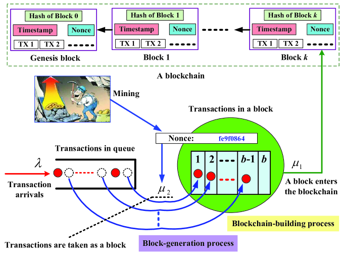
Now, from Figure 1 we provide some model descriptions as follows:

Arrival process: Transactions arrive at the blockchain system according to a Poisson process with arrival rate $\lambda$. Each transaction must first enter and queue up in an waiting room of infinite size. Note that the arrival process of transactions is denoted in the lower left corner of Figure 1.

Service process: Each arrival transaction first queues up in the waiting room. Then it waits for being successfully mined into a block, this is regarded as the first stage of service, called block generation. Until the block-generation time, a group of transactions are chosen as a block and simultaneously, a nonce is appended to the block by the mining winner. See the lower middle part of Figure 1 for more details. Finally, the block with the group of transactions will be pegged to a blockchain, this is regarded as the second stage of service due to the network latency, called blockchain building, see the right and lower part of Figure 1. In addition, the upper part of Figure 1 also outlines the blockchain and the internal structure of every block.

In the blockchain system, for the two stages of services, we assume that the block-generation times in the first stage are i.i.d and exponential with service rate $\mu_{2}$; the blockchain-building times in the second stage are i.i.d and exponential with the service rate $\mu_{1}$.

The block-generation discipline: A block can consist of several transactions but at most $b$ transactions. The transactions mined into a block are not completely based on the First Come First Service (FCFS) with respect to the transaction arrivals. Thus some transactions in the back of this queue may be preferentially first chosen into the block, seen in the lower middle part of Figure 1.

For simplification of description, our later computation will be based on the FCFS discipline. This may be a better approximation in analysis of the blockchain queueing system if the transactions are regarded as the indistinctive ones under a dynamic behavior setting.

The maximum block size: To avoid the spam attack, the maximum block size is limited. We assume that there are at most $b$ transactions in each block. If the resulting block size is smaller than the maximum block size $b$, then the transactions newly arriving during the mining process of a block can be accepted in the block again. If there are more than $b$ transactions in the waiting room, then a new block will include $b$ transactions through the full blocks to maximize the batch service ability in the blockchain system.

Independence: We assume that all the random variables defined above are independent of each other.

Remark 1: The arrival process of transactions at the blockchain system may be non-Poisson (for example, Markov arrival process, renewal process and nonhomogeneous Poisson process). On the other hand, the two stages of batch service times may be non-exponential (for example, phase-type distribution and general distribution). However, so far analysis of the blockchain queues with renewal arrival process or with general service time distribution has still been an interesting open problem in queueing research of blockchain systems.

Remark 2: In the blockchain system, there are key factors, such as the maximum block size, mining reward, transaction fee, mining strategy, security of blockchain and so on. Based on some of them, we may develop reward queueing models, decision queueing models, and game queueing models in the study of blockchain systems. Analysis for these key factors will be very necessary and useful in improving blockchain technologies in many future applications.

3 A Markov Process of GI/M/1 Type

In this section, for the blockchain queueing system, we establish a continuous-time Markov process of GI/M/1 type. Based on this, we derive a system stable condition and the stationary probability vector of this system by means of the matrix-geometric solution.

Let $I\left(t\right)$ and$\ J\left(t\right)$ be the numbers of transactions in the block and in the queue at time $t$, respectively. Then, $\left(I\left(t\right),J\left(t\right)\right)$ may be regarded as a state of the blockchain queueing system at time $t$. Note that $i=0,1,\ldots,b$ and $j=0,1,2,\ldots$, for various cases of $\left(I\left(t\right),J\left(t\right)\right)$ we write

$$\mathbf{\Omega}= \left\{\left(i,j\right):i=0,1,\ldots,b,\ \ \ j=0,1,2,\ldots\right\}$$

$$= \left\{\left(0,0\right),\left(1,0\right),\ldots,\left(b,0\right);\left(0,1\right),\left(1,1\right),\ldots,\left(b,1\right);\ldots;\right.$$

$$\left.\left(0,b\right),\left(1,b\right),\ldots,\left(b,b\right);\left(0,b+1\right),\left(1,b+1\right),\ldots,\left(b,b+1\right);\ldots\right\}.$$ (1)

Figure 2: State transition relation of a Markov process

Let $X\left(t\right)=\left(I\left(t\right),J\left(t\right)\right)$. Then $\left\{X\left(t\right):t\geq 0\right\}$ is a continuous-time Markov process of GI/M/1 type on the state space $\mathbf{\Omega}$. Figure 2 denotes the state transition relation of the Markov process $\left\{X\left(t\right):t\geq 0\right\}$, thus its infinitesimal generator is given by

$$\bm{Q}=\left(\begin{array}[]{ccccccccc}B_{0}&A_{0}&&&&&&&\\ B_{1}&A_{1}&A_{0}&&&&&&\\ B_{2}&&A_{1}&A_{0}&&&&&\\ \vdots&&&\ddots&\ddots&&&&\\ B_{b}&&&&A_{1}&A_{0}&&&\\ &A_{b}&&&&A_{1}&A_{0}&&\\ &&A_{b}&&&&A_{1}&A_{0}&\\ &&&\ddots&&&&\ddots&\ddots\end{array}\right),$$ (2)

where

$$A_{0}=\lambda I,\ \ A_{1}=\left(\begin{array}[]{cccc}-\left(\lambda+\mu_{2}\right)&&&\\ \mu_{1}&-\left(\lambda+\mu_{1}\right)&&\\ \vdots&&\ddots&\\ \mu_{1}&&&-\left(\lambda+\mu_{1}\right)\end{array}\right),A_{b}=\left(\begin{array}[]{cccc}0&\cdots&0&\mu_{2}\\ &&&\\ &&&\\ &&&\end{array}\right),$$

and

$$B_{0}=\left(\begin{array}[]{cccc}-\lambda&&&\\ \mu_{1}&-\left(\lambda+\mu_{1}\right)&&\\ \vdots&&\ddots&\\ \mu_{1}&&&-\left(\lambda+\mu_{1}\right)\end{array}\right),$$

$$B_{1}=\left(\begin{array}[]{ccccc}0&\mu_{2}&0&\cdots&0\\ &&&&\\ &&&&\\ &&&&\end{array}\right),\ \ B_{2}=\left(\begin{array}[]{ccccc}0&0&\mu_{2}&\cdots&0\\ &&&&\\ &&&&\\ &&&&\end{array}\right),\ \ \ldots,\ \ B_{b}=\left(\begin{array}[]{cccc}0&\cdots&0&\mu_{2}\\ &&&\\ &&&\\ &&&\end{array}\right).$$

For the continuous-time Markov process of GI/M/1 type, now we use the mean drift method to discuss its system stable condition. Note that the mean drift method for checking system stability is given a detailed introduction in Chapter 3 of Li [18] (e.g., Theorem 3.19 and the continuous-time case in Page 172).

From Chapter 1 of Neuts [24] or Chapter 3 of Li [18], for the Markov process of GI/M/1 type, we write

$$A=A_{0}+A_{1}+A_{b}=\left(\begin{array}[]{ccccc}-\mu_{2}&&&&\mu_{2}\\ \mu_{1}&-\mu_{1}&&&\\ \vdots&&\ddots&&\\ \mu_{1}&&&-\mu_{1}&\\ \mu_{1}&&&&-\mu_{1}\end{array}\right).$$

Clearly, the Markov process $A$ with finite states is irreducible, aperiodic and positive recurrent. In this case, we write its stationary probability vector as $\bm{\theta}=\left(\theta_{0},\theta_{1},\ldots,\theta_{b}\right)$. Also, $\bm{\theta}$ is the unique solution to the system of linear equations: $\bm{\theta}A=\bm{0}$ and $\bm{\theta}\bm{e}=1$, where $\bm{e}$ is a column vector of ones with proper dimension. It is easy to check that

$$\bm{\theta}=\left(\frac{\mu_{1}}{\mu_{1}+\mu_{2}},0,\ldots,0,\frac{\mu_{2}}{\mu_{1}+\mu_{2}}\right).$$

The following theorem provides a necessary and sufficient condition under which the Markov process $\bm{Q}$ is positive recurrent.

Theorem 1

The Markov process $\bm{Q}$ of GI/M/1 type is positive recurrent if and only if

$$\frac{b\mu_{1}\mu_{2}}{\mu_{1}+\mu_{2}}>\lambda.$$

Proof

By using the mean drift method given in Chapter 3 of Li [18] (e.g., Theorem 3.19 and the continuous-time case in Page 172), it is easy to see that the Markov process $\bm{Q}$ of GI/M/1 type is positive recurrent if and only if

$$\bm{\theta}A_{0}\bm{e}<b\bm{\theta}A_{b}\bm{e}.$$ (3)

Note that

$$\bm{\theta}A_{0}\bm{e}=\lambda,$$ (4)

and

$$b\bm{\theta}A_{b}\bm{e}=b\theta_{0}\mu_{2}=\frac{b\mu_{1}\mu_{2}}{\mu_{1}+\mu_{2}},$$ (5)

thus we obtain

$$\frac{b\mu_{1}\mu_{2}}{\mu_{1}+\mu_{2}}>\lambda.$$

This completes the proof.  

When the Markov process $\bm{Q}$ of GI/M/1 type is positive recurrent, we write its stationary probability vector as

$$\bm{\pi}=\left(\bm{\pi}_{0},\bm{\pi}_{1},\bm{\pi}_{2},\ldots\right),$$

where

$$\bm{\pi}_{0} =\left(\pi_{0,0},\pi_{1,0},\ldots,\pi_{b,0}\right),$$

$$\bm{\pi}_{1} =\left(\pi_{0,1},\pi_{1,1},\ldots,\pi_{b,1}\right),$$

$$\bm{\pi}_{k} =\left(\pi_{0,k},\pi_{1,k},\ldots,\pi_{b,k}\right),\ \ \ k\geq 2.$$

For the Markov process $\bm{Q}$ of GI/M/1 type, to compute its stationary probability vector, we need to first obtain the rate matrix $R$, which is the minimal nonnegative solution to the following nonlinear matrix equation

$$R^{b}A_{b}+RA_{1}+A_{0}=\mathbf{0}.$$ (6)

In general, it is very complicated to provide expression for the unique solution to this nonlinear matrix equation due to the term $R^{b}A_{b}$ of size $b+1$. In fact, for the blockchain queueing system, here we can not also provide an explicit expression for the rate matrix $R$. For example, we consider a special case with $b=2$. For this simple case, we have

$$A_{0}=\lambda I,A_{1}=\left(\begin{array}[]{ccc}-\left(\lambda+\mu_{2}\right)&&\\ \mu_{1}&-\left(\lambda+\mu_{1}\right)&\\ \mu_{1}&&-\left(\lambda+\mu_{1}\right)\end{array}\right),A_{2}=\left(\begin{array}[]{ccc}0&0&\mu_{2}\\ &&\\ &&\end{array}\right).$$

From computing $R^{2}A_{2}+RA_{1}+A_{0}=\mathbf{0}$, it is easy to see that for the simple case with the maximal block size $b=2$, we can not provide an explicit expression for the rate matrix $R$ of size $3$ yet.

Although the rate matrix $R$ has not an explicit expression, we can use some iterative algorithms, given in Chapters 1 and 2 of Neuts [24], to give its numerical solution. Here, an effective iterative algorithm is described as

$$R_{0} =\mathbf{0,}$$

$$R_{N+1} =\left(R_{N}^{b}A_{b}+A_{0}\right)\left(-A_{1}\right)^{-1}.$$

Note that this algorithm is fast convergent, that is, after a finite number of iterative steps, we can numerically given a solution of higher precision for the rate matrix $R$.

The following theorem directly comes from Theorem 1.2.1 of Chapter 1 in Neuts [24]. Here, we restate it without a proof.

Theorem 2

If the Markov process $\bm{Q}$ of GI/M/1 type is positive recurrent, then the stationary probability vector $\bm{\pi}=\left(\bm{\pi}_{0},\bm{\pi}_{1},\bm{\pi}_{2},\ldots\right)$ is given by

$$\bm{\pi}_{k}=\bm{\pi}_{0}R^{k},\ \ \ k\geq 1,$$ (7)

where the vector $\bm{\pi}_{0}$ is positive, and it is the unique solution to the following system of linear equations:

$$\left.\bm{\pi}_{0}B\left[R\right]=\bm{\pi}_{0},\right.$$ (8)

$$\left.\bm{\pi}_{0}\left(I-R\right)^{-1}\bm{e}=1,\right.$$

and the matrix $B\left[R\right]=\sum\nolimits_{k=0}^{b}R^{k}B_{k}$ is irreducible and stochastic.

4 Performance Analysis

In this section, we provide performance analysis of the blockchain queueing system. To this end, we provide three key performance measures and give their simple expressions by means of the vector $\bm{\pi}_{0}$ and the rate matrix $R$. Finally, we use numerical examples to verify computability of our theoretical results, and show how the performance measures depend on some key parameters of this system.

When the blockchain queueing system is stable, we write

$$I=lim_{t\rightarrow+\infty}I\left(t\right),\ \ \ J=lim_{t\rightarrow+\infty}J\left(t\right).$$

(a) The average number of transactions in the queue

It follows from (8) and (7) that

$$E\left[J\right]=\overset{\infty}{\underset{j=0}{\sum}}j\overset{b}{\underset{i=0}{\sum}}\pi_{i,j}=\overset{\infty}{\underset{j=0}{\sum}}j\bm{\pi}_{j}\bm{e}=\bm{\pi}_{0}R\left(I-R\right)^{-2}\bm{e}.$$

(b) The average number of transactions in the block

Let $\bm{h}=\left(0,1,2,\ldots,b\right)^{T}$. Then

$$E\left[I\right]=\overset{\infty}{\underset{j=0}{\sum}}\underset{i=0}{\overset{b}{\sum}}i\pi_{i,j}=\underset{j=0}{\overset{\infty}{\sum}}\bm{\pi}_{j}\bm{h}=\bm{\pi}_{0}\left(I-R\right)^{-1}\bm{h}.$$

(c) The average transaction-confirmation time

In the blockchain system, the transaction-confirmation time is the time interval from the time epoch that a transaction arrives at the waiting room to the point that the blockchain pegs a block with this transaction. In fact, the transaction-confirmation time is the sojourn time of the transaction in the blockchain system, and it is also the sum of the block-generation and blockchain-building times of a block with this transaction.

Let $T$ denote the transaction-confirmation time of any transaction when the blockchain system is stable.

The following theorem provides expression for the average transaction-confirmation time by means of the stationary probability vector.

Theorem 3

If the blockchain queueing system is stable, then the average transaction-confirmation time $E[T]$ is given by

$$E[T]=\overset{\infty}{\underset{k=0}{\sum}}\overset{b-1}{\underset{l=0}{\sum}}\pi_{0,kb+l}\left(k+1\right)\left(\frac{1}{\mu_{1}}+\frac{1}{\mu_{2}}\right)+\overset{b}{\underset{i=1}{\sum}}\overset{\infty}{\underset{k=0}{\sum}}\overset{b-1}{\underset{l=0}{\sum}}\pi_{i,kb+l}\left[\frac{1}{\mu_{1}}+\left(k+1\right)\left(\frac{1}{\mu_{1}}+\frac{1}{\mu_{2}}\right)\right].$$

Proof

It is clear that $\left(i,kb+l\right)$ is a state of the blockchain system for $i=0,1,\ldots,b,k=0,1,\ldots,$ and $l=0,1,\ldots,b-1.$

When a transaction arrives at the blockchain system at time $t$, it observes and finds that there are $i$ transactions in the block and $kb+l$ transactions in the queue. Based on the two stages of exponential service times and by using the stationary probability vector $\bm{\pi}$, we apply the law of total probability to be able to compute the average transaction-confirmation time. For this, our computation will have two different cases as follows:

Case one: $i=0$. In this case, the transaction finds that there is no transaction in the block at the beginning moment, thus its transaction-confirmation time includes $k+1$ block-generation times $(k+1)/\mu_{2}$ and $k+1$ blockchain-building times $(k+1)/\mu_{1}$. Thus we obtain

$$E[T_{|i=0}]=\overset{\infty}{\underset{k=0}{\sum}}\overset{b-1}{\underset{l=0}{\sum}}\pi_{0,kb+l}\left(k+1\right)\left(\frac{1}{\mu_{1}}+\frac{1}{\mu_{2}}\right).$$

Case two: $i=1,2,\ldots,b$. In this case, the transaction finds that there are $i$ transactions in the block, thus its transaction-confirmation time includes $k+1$ block-generation times $(k+1)/\mu_{2}$ and $k+2$ blockchain-building times $(k+2)/\mu_{1}$. We obtain

$$E[T_{|i\neq 0}]=\overset{b}{\underset{i=1}{\sum}}\overset{\infty}{\underset{k=0}{\sum}}\overset{b-1}{\underset{l=0}{\sum}}\pi_{i,kb+l}\left[\frac{1}{\mu_{1}}+\left(k+1\right)\left(\frac{1}{\mu_{1}}+\frac{1}{\mu_{2}}\right)\right].$$

Therefore, by means of considering all the different cases, the average transaction-confirmation time $E[T]$ is given by

$$E[T]=\overset{\infty}{\underset{k=0}{\sum}}\overset{b-1}{\underset{l=0}{\sum}}\pi_{0,kb+l}\left(k+1\right)\left(\frac{1}{\mu_{1}}+\frac{1}{\mu_{2}}\right)+\overset{b}{\underset{i=1}{\sum}}\overset{\infty}{\underset{k=0}{\sum}}\overset{b-1}{\underset{l=0}{\sum}}\pi_{i,kb+l}\left[\frac{1}{\mu_{1}}+\left(k+1\right)\left(\frac{1}{\mu_{1}}+\frac{1}{\mu_{2}}\right)\right].$$

This completes the proof.  

Let $\langle\mathbf{x}\rangle_{|_{i=0}}$ be the 1st element of the vector $\mathbf{x}$. The following theorem provides a simple expression for the average transaction-confirmation time $E[T]$ by means of the vector $\bm{\pi}_{0}$ and the rate matrix $R$.

Theorem 4

If the blockchain queueing system is stable, then the average transaction-confirmation time $E[T]$ is given by

$$E\left[T\right] = \frac{1}{\mu_{1}}\left[\bm{\pi}_{0}\left(I-R\right)^{-1}\bm{e}-\left\langle\bm{\pi}_{0}\left(I-R\right)^{-1}\right\rangle_{|_{i=0}}\right]$$

$$+\left(\frac{1}{\mu_{1}}+\frac{1}{\mu_{2}}\right)\bm{\pi}_{0}\left(I-R^{b}\right)^{-1}\left(I-R\right)^{-1}\bm{e}.$$

Proof

By using Theorem 3, we give some corresponding computation. Note that

$$\frac{1}{\mu_{1}}\overset{b}{\underset{i=1}{\sum}}\overset{\infty}{\underset{k=0}{\sum}}\overset{b-1}{\underset{l=0}{\sum}}\pi_{i,kb+l}=\frac{1}{\mu_{1}}\left[\overset{\infty}{\underset{k=0}{\sum}}\overset{b-1}{\underset{l=0}{\sum}}\bm{\pi}_{kb+l}\bm{e}-\overset{\infty}{\underset{k=0}{\sum}}\overset{b-1}{\underset{l=0}{\sum}}\pi_{0,kb+l}\right],$$

$$\overset{\infty}{\underset{k=0}{\sum}}\overset{b-1}{\underset{l=0}{\sum}}\bm{\pi}_{kb+l}\bm{e}=\overset{\infty}{\underset{k=0}{\sum}}\overset{b-1}{\underset{l=0}{\sum}}\bm{\pi}_{0}R^{kb+l}\bm{e}=\bm{\pi}_{0}\left(I-R\right)^{-1}\bm{e},$$

$$\overset{\infty}{\underset{k=0}{\sum}}\overset{b-1}{\underset{l=0}{\sum}}\pi_{0,kb+l}=\left\langle\overset{\infty}{\underset{k=0}{\sum}}\overset{b-1}{\underset{l=0}{\sum}}\bm{\pi}_{kb+l}\right\rangle_{|_{i=0}}=\left\langle\bm{\pi}_{0}\left(I-R\right)^{-1}\right\rangle_{|_{i=0}},$$

we obtain

$$\frac{1}{\mu_{1}}\overset{b}{\underset{i=1}{\sum}}\overset{\infty}{\underset{k=0}{\sum}}\overset{b-1}{\underset{l=0}{\sum}}\pi_{i,kb+l}=\frac{1}{\mu_{1}}\left[\bm{\pi}_{0}\left(I-R\right)^{-1}\bm{e}-\left\langle\bm{\pi}_{0}\left(I-R\right)^{-1}\right\rangle_{|_{i=0}}\right].$$

On the other hand, since

$$\overset{b}{\underset{i=0}{\sum}}\overset{\infty}{\underset{k=0}{\sum}}\overset{b-1}{\underset{l=0}{\sum}}\pi_{i,kb+l}\left(k+1\right)\left(\frac{1}{\mu_{1}}+\frac{1}{\mu_{2}}\right)=\left(\frac{1}{\mu_{1}}+\frac{1}{\mu_{2}}\right)\overset{\infty}{\underset{k=0}{\sum}}\overset{b-1}{\underset{l=0}{\sum}}\left(k+1\right)\bm{\pi}_{kb+l}\bm{e},$$

we get

$$\overset{\infty}{\underset{k=0}{\sum}}\overset{b-1}{\underset{l=0}{\sum}}\left(k+1\right)\bm{\pi}_{kb+l}=\overset{\infty}{\underset{k=0}{\sum}}\overset{b-1}{\underset{l=0}{\sum}}\left(k+1\right)\bm{\pi}_{0}R^{kb+l}$$

$$= \bm{\pi}_{0}\overset{\infty}{\underset{k=0}{\sum}}\left(k+1\right)R^{kb}\left(I-R^{b}\right)\left(I-R\right)^{-1}$$

$$= \bm{\pi}_{0}\left(I-R^{b}\right)^{-1}\left(I-R\right)^{-1}.$$

This leads our desired result. The proof is completed.  

In the remainder of this section, we provide some numerical examples to verify computability of our theoretical results and to analyze how the three performance measures $E\left[J\right]$, $E\left[I\right]$ and $E\left[T\right]$ depend on some crucial parameters of the blockchain queueing system.

In the numerical examples, we take some common parameters: Block-generation service rate $\mu_{1}\in\left[0.05,1.5\right]$, blockchain-building service rate $\mu_{2}=2$, arrival rate $\lambda=0.3$, maximum block size $b_{1}=40,b_{2}=80,b_{3}=320$.

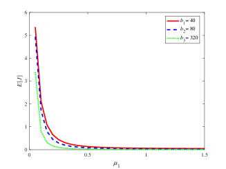
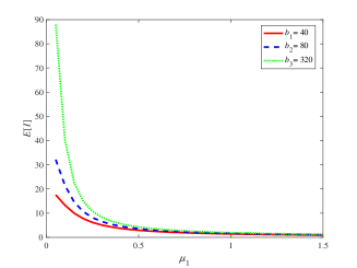
From the left part of Figure 3, it is seen that $E\left[J\right]$ and $E\left[I\right]$ decrease, as $\mu_{1}$ increases. At the same time, from the right part of Figure 3, $E\left[J\right]$ decreases as $b$ increases, but $E\left[I\right]$ increases as $b$ increases.

Figure 3: $E\left[J\right]$, $E\left[I\right]$ vs. $\mu_{1}$ for three different $b_{1},b_{2},b_{3}$.

From Figure 4, it is seen that $E\left[T\right]$ decreases, as $\mu_{1}$ increases; while it decreases, as $b$ increases.

Figure 4: $E\left[T\right]$ vs. $\mu_{1}$ for three different $b_{1},b_{2},b_{3}$.

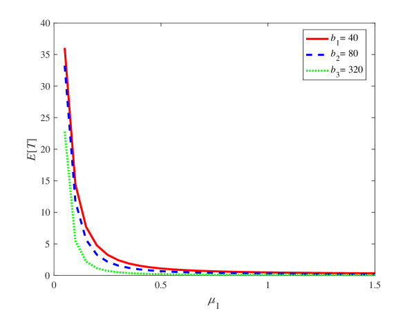
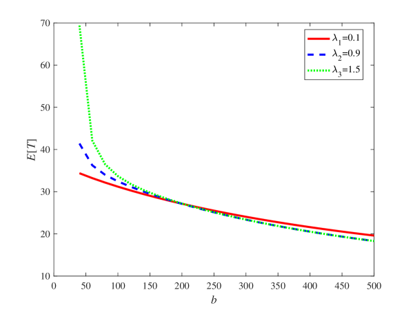
Finally, we specifically observe the impact of the maximal block size $b$ on the $E\left[T\right]$. Comparing with the parameters given in Figures 3 and 4, we only change the two parameters $b$ and $\lambda$: $b=40,41,42,\ldots,500$, $\lambda_{1}=0.1,\lambda_{2}=0.9,\lambda_{3}=1.5$. From Figure 5, it is seen that $E\left[T\right]$ decreases, as $b$ increases. In addition, it is observed that there exists a critical value $\eta$ such that when $b\leq\eta$, $E\left[T\right]$ increases, as $\lambda$ increases. On the contrary, when $b>\eta$, $E\left[T\right]$ increases, as $\lambda$ decreases. In fact, such a difference is also intuitive that the block generation time becomes bigger as $\lambda$ decreases.

Figure 5: $E\left[T\right]$ vs. $b$ for three different $\lambda_{1},\lambda_{2},\lambda_{3}$.

5 Concluding Remarks

In this paper, our aim is to focus on how to develop queueing theory of blockchain systems. To do this, we design an interesting Markovian batch-service queueing system with two different service stages, while the two stages can well express the mining process in the miners pool and the building of a new blockchain. By using the matrix-geometric solution, we not only obtain a system stable condition but also simply express three key performance measures: The average number of transactions in the queue, the average number of transactions in a block, and the average transaction-confirmation time. Finally, we use numerical examples to verify computability of our theoretical results. Along these lines, we will continue our future research on the following directions:

– Considering more general blockchain queueing systems, for example, the Markov arrival process of transactions, and two stages of phase-type batch services.

– Analyzing multiple classes of transactions in the blockchain systems. Also, the transactions are dealt with in the block-generation and blockchain-building processes according to a priority service discipline.

– When the arrivals of transactions are a renewal process, and the block-generation times or the blockchain-building times follow general probability distributions, an interesting research work is to focus on fluid and diffusion approximations of the blockchain systems.

– Setting up reward function with respect to cost structures, transaction fees, mining reward, consensus mechanism, security and so forth. Our aim is to find optimal policies in the blockchain systems.

– Further developing stochastic optimization and control, Markov decision processes and stochastic game theory in the blockchain systems.

References

- [1] Beck, R., Avital, M., Rossi, M., Thatcher, J.B.: Blockchain technology in business and information systems research. Business & Information Systems Engineering 59(6), 381–384 (2017)
- [2] Bhaskar, N.D., Chuen, D.L.K.: Bitcoin mining technology. In: Handbook of Digital Currency, pp. 45–65 (2015)
- [3] Biais, B., Bisiere, C., Bouvard, M., Casamatta, C.: The blockchain folk theorem. Working paper, Toulouse School of Economics, Université Toulouse Capitole, pp. 1–71 (2018)
- [4] Böhme, R., Christin, N., Edelman, B., Moore, T.: Bitcoin: Economics, technology, and governance. Journal of Economic Perspectives 29(2), 213–38 (2015)
- [5] Catalini, C., Gans, J.S.: Some simple economics of the blockchain. National Bureau of Economic Research, No. w22952, pp. 1–29 (2016)
- [6] Constantinides, P., Henfridsson, O., Parker, G.G.: Introduction – Platforms and infrastructures in the digital age. Information Systems Research 29(2), 381–400 (2018)
- [7] Davidson, S., De Filippi, P., Potts, J.: Economics of blockchain. Online Available: HAL Id: hal-01382002, pp. 1–23 (2016)
- [8] Debus, J.: Consensus methods in blockchain systems. Frankfurt School of Finance & Management, Blockchain Center, Technical Report, pp. 1–58 (2017)
- [9] Dinh, T.T.A., Liu, R., Zhang, M., Chen, G., Ooi, B.C., Wang, J.: Untangling blockchain: A data processing view of blockchain systems. IEEE Transactions on Knowledge and Data Engineering 30(7), 1366–1385 (2018)
- [10] Foroglou, G., Tsilidou, A.L.: Further applications of the blockchain. Abgerufen Am 3, 1–9 (2015)
- [11] Houy, N.: The bitcoin mining game. Online Available: HAL Id: halshs-00958224, pp. 1–17 (2014)
- [12] Huckle, S., Bhattacharya, R., White, M., Beloff, N.: Internet of Things, blockchain and shared economy applications. Procedia Computer Science 98, 461-466 (2016)
- [13] Kasahara, S., Kawahara, J.: Effect of Bitcoin fee on transaction-confirmation process. arXiv preprint arXiv:1604.00103, pp. 1–24 (2016)
- [14] Kawase, Y., Kasahara, S.: Transaction-confirmation time for Bitcoin: A queueing analytical approach to blockchain mechanism. In: International Conference on Queueing Theory and Network Applications, pp. 75–88. Springer (2017)
- [15] Kiayias, A., Koutsoupias, E., Kyropoulou, M., Tselekounis, Y.; Blockchain mining games. In: Proceedings of the 2016 ACM Conference on Economics and Computation, pp. 365–382. ACM (2016)
- [16] Kondor, D., Pósfai, M., Csabai, I., Vattay, G.: Do the rich get richer? An empirical analysis of the Bitcoin transaction network. PloS one 9(2), 1–10 (2014)
- [17] Lewenberg, Y., Bachrach, Y., Sompolinsky, Y., Zohar, A., Rosenschein, J.S.: Bitcoin mining pools: A cooperative game theoretic analysis. In: Proceedings of the 2015 International Conference on Autonomous Agents and Multiagent Systems, pp. 919–927 (2015)
- [18] Li, Q.L.: Constructive Computation in Stochastic Models with Applications: The RG-Factorizations. Springer (2010)
- [19] Lin, I.C., Liao, T.C.: A survey of blockchain security issues and challenges. International Journal of Network Security 19(5), 653–659 (2017).
- [20] Lindman, J., Tuunainen, V.K., Rossi, M.: Opportunities and risks of blockchain technologies – a research agenda. In: Proceedings of the 50th Hawaii International Conference on System Sciences, pp. 1533–1542 (2017)
- [21] Mettler, M.: Blockchain technology in healthcare: The revolution starts here. In: The 18th International IEEE Conference on e-Health Networking, Applications and Services, pp. 1–3. IEEE (2016)
- [22] Montemayor, L., Boersma, T., van Dorp, T.: Comprehensive guide to companies involved in blockchain and energy. Blockchain Business. (2018)
- [23] Nakamoto, S.: Bitcoin: A peer-to-peer electronic cash system. pp. 1–9 (2008). [Online]. Available: https://bitcoin.org/bitcoin.pdf
- [24] Neuts, M.F.: Matrix-Geometric Solutions in Stochastic Models. Johns Hopkins University Press (1981)
- [25] NRI, Survey on blockchain technologies and related services. FY2015 Report, Nomura Research Institute, pp. 1–78 (2015). [Online]. Available: http://www.meti.go.jp/english/press/2016/pdf/0531 01f.pdf
- [26] Ober, M., Katzenbeisser, S., Hamacher, K.: Structure and anonymity of the Bitcoin transaction graph. Future Internet 5(2), 237–250 (2013)
- [27] Plansky, J., O’Donnell, T., Richards, K.: A strategist’s guide to blockchain. Strategy + Business Magazine 82, 1–12 (2016)
- [28] Risius, M., Spohrer, K.: A blockchain research framework. Business & Information Systems Engineering 59(6), 385–409 (2017)
- [29] Swan, M.: Blockchain: Blueprint for a new economy. O’Reilly Media, Inc. (2015)
- [30] Tsai, W.T., Blower, R., Zhu, Y., Yu, L.: A system view of financial blockchains. In: The IEEE Symposium on Service-Oriented System Engineering, pp. 450–457. IEEE (2016)
- [31] Tschorsch, F., Scheuermann, B.: Bitcoin and beyond: A technical survey on decentralized digital currencies. IEEE Communications Surveys & Tutorials 18(3), 2084–2123 (2016)
- [32] Vranken, H.: Sustainability of Bitcoin and blockchains. Current Opinion in Environmental Sustainability 28, 1–9 (2017)
- [33] Wang, W., Hoang, D.T., Xiong, Z., Niyato, D., Wang, P., Hu, P., Wen, Y.: A survey on consensus mechanisms and mining management in blockchain networks. arXiv preprint arXiv:1805.02707, pp. 1–33 (2018)
- [34] Yli-Huumo, J., Ko, D., Choi, S., Park, S., Smolander, K.: Where is current research on blockchain technology? — A systematic review. PloS one 11(10), 1–27 (2016)
- [35] Zheng, Z., Xie, S., Dai, H.N., Chen, X., Wang, H.: An overview of blockchain technology: Architecture, consensus, and future trends. In: The IEEE International Congress on Big Data, pp. 557–564. IEEE (2017)
- [36] Zheng, Z., Xie, S., Dai, H.N., Wang, H.: Blockchain challenges and opportunities: A survey. International Journal of Web and Grid Services 13(2), 1–25 (2017)