Quantifying Deployability & Evolvability of Future Internet Architectures via Economic Models

Abstract

Emerging new applications demand the current Internet to provide new functionalities. Although many future Internet architectures and protocols have been proposed to fulfill such needs, ISPs have been reluctant to deploy many of these architectures. We believe technical issues are not the main reasons as many of these new proposals are technically sound. In this paper, we take an economic perspective and seek to answer: Why do most new Internet architectures fail to be deployed? How can the deployability of a new architecture be enhanced? We develop a game-theoretic model to characterize the outcome of an architecture’s deployment through the equilibrium of ISPs’ decisions. This model enables us to: (1) analyze several key factors of the deployability of a new architecture such as the number of critical ISPs and the change of routing path; (2) explain the deploying outcomes of some previously proposed architectures/protocols such as IPv6, DiffServ, CDN, etc., and shed light on the “Internet flattening phenomenon”; (3) predict the deployability of a new architecture such as NDN, and compare its deployability with competing architectures. Our study suggests that the difficulty to deploy a new Internet architecture comes from the “coordination” of distributed ISPs. Finally, we design a mechanism to enhance the deployability of new architectures.

I Introduction

Emerging applications create a constant push for the Internet to be “evolvable” to provide new functionalities. For example, streaming video traffic from Netflix and other services requires highly efficient content delivery across the Internet. Also, users of online social network services like Facebook want their private chats to be securely protected. The increasing number of mobile phones and IoT devices require better mobility and security support, and so on. However, many of these needs are not being supported by the IPv4 network. To meet these emerging needs, researchers have been developing new architectures and protocols, and more importantly, exploring how to make the Internet “evolvable” so as to incorporate new functionalities. Unfortunately, many of these research efforts ultimately fail to result in wide scale deployment.

Different Internet architectures/protocols experience different degrees of deployment difficulties. In the 1990s, the protocol IP version 6 (IPv6) was introduced to overcome certain shortcomings of IP version 4. In particular, IPv6 provides a larger address space and additional features such as security. However, after more than 20 years of effort, only a minority of current Internet traffic is based on IPv6 [ipv6_stat]. Differentiated service (DiffServ)[diff_serv] was designed to provide Quality of Service (QoS) guarantees. Although it is supported by many commercial routers [diff_serv], only a few Internet service providers (ISPs) are willing to turn on the DiffServ function. In contrast, content delivery network (CDN) technology has enjoyed rapid growth and wide deployment; at the time of this writing, over 50% of the Internet traffic is delivered by CDNs [cdn_stat]. In the past decade, a number of novel Internet architectures were proposed to address challenges in the the current IP network, through substantial changes to the network protocols. For example, Named-Data Networking (NDN) [ndn] natively facilitates content distribution, while the eXpressive Internet Architecture (XIA) [xia] enables incremental deployment of future protocols and features intrinsic security. MobilityFirst[mobilityfirst] provides first-class support for mobile devices. Although NDN, XIA and MobilityFirst all have functional prototype systems, as of this moment they do not have the wide-scale deployment.

All of the above architecture/protocol proposals claimed to improve the current Internet if they are successfully deployed. However, only the CDN technology is smoothly deployed in the Internet, while most of the others are not. This motivates us to explore: Why do many new Internet architectures fail to be deployed? How can the deployability of a new architecture/protocol be enhanced? The failure of many proposed architectures/protocols to reach wide deployment is probably not due to technical issues. In fact, many of these proposed architectures feature technically superior designs, compared to the present IPv4 network. Instead, economic factors are crucial in determining the deployability of a new Internet architecture/protocol.

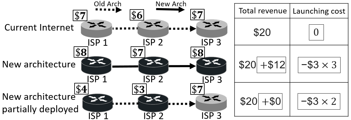
Figure 1: Economic difficulty to deploy a new Internet architecture

To illustrate, let us consider the following example. Fig. 1 depicts a simple network with three ISPs, and a traffic flow from ISP 1 to ISP 3. Suppose that under the current Internet architecture, the whole network can gain a total revenue of $20. Assume that a new Internet architecture, if it is fully deployed, will increase the total revenue of the whole network to $32 (i.e., improve the revenue by $12). Each ISP has a launching cost of $3 to deploy this new architecture. Suppose the revenue improvement is evenly distributed among ISPs, i.e., each ISP gains $12/3=$4, or each ISP will earn $4 more by investing $3 to upgrade the architecture, which yields a net gain of $4-$3=$1. However, the deployment requires a “full-path” participation, i.e. ISP 1, ISP 2 and ISP 3 all need to deploy the new architecture in order to achieve the improved functionality. Fig. 1 shows that when only ISP 1 and ISP 2 deploy (ISP 3 does not), the total revenue will not be improved, because the new functionality is not enabled.

Although the above example illustrates the potential profit gain for each ISP, unfortunately, the new architecture will not necessarily be deployed in the network. The reason is no ISP can be certain of gaining the benefit by deploying the new architecture unilaterally. In fact, if an ISP deploys, it will gain $1 only if the other two ISPs also deploy; otherwise the ISP will lose $3. The main difficulty is that each ISP is uncertain about other ISPs’ deployment decisions. Given this uncertainty, ISPs tend to be conservative, and this leads to the failure of deployment. The above example highlights that a new Internet architecture can be difficult to deploy even if it can bring higher profits.

This paper studies the economic issues for the deployment of new Internet architecture/protocol, and we aim to answer:

• Why have many Internet architectures/protocols (e.g., IPv6, NDN, XIA) failed to achieve large scale acceptance and wide deployment by ISPs?

• What are the key factors that influence the deployability of a new architecture/protocol? How to enhance the deployability of a new architecture/protocol?

In addition, we analyze the economic impact of some engineering mechanisms, e.g., tunneling, that have been proposed to support incremental deployment of new Internet architectures. We also study the “Internet flattening phenomenon”, where content providers are bypassing transit ISPs and instead placing their servers in data centers close to the end users.

Our contributions are:

• We present a game-theoretic model of ISPs’ economic interactions regarding the deployment decisions of a new Internet architecture (Sec. II). Our model captures realistic factors, e.g., the routing paths can change during the deployment. We later extend the model to compare the deployability of competing architectures and study which will eventually get deployed (Sec. V).

• We analyze ISPs’ deployment decisions via the notion of “equilibrium” when ISPs have uncertainties on the benefits of the new architecture and are risk-neutral.

• We identify factors that make an architecture difficult to deploy. Our analysis suggests that the requirement for many ISPs to coordinate is an important hurdle for deployability. It explains why architectures like IPv6 or DiffServ are difficult to deploy, while deploying CDN and NAT is easy. Furthermore, the change of routing path and the competition between the old and the new architectures are not major factors hindering deployment.

• We study several alternatives to enhance the deployability of a new architecture. We quantify how incremental deployment mechanisms such as IPv6 tunneling improve the deployability of an architecture (Sec. IV-C). Our model confirms that by relying on data centers, content providers can more easily deploy new architectures in the flattened Internet. Lastly, we design a coordination mechanism to improve the deployability of new architectures (Sec. VI).

The organization of this paper is as follows. In Section II, we model the ISP-network and the cost/benefits for ISPs to deploy a new architecture, and formulate a strategic game. In Section III, we reason about ISPs’ behaviors on deployment. In Section IV, we analyze the impact of different factors on the deployability of an architecture. Section V presents an extension of the model to consider partial deployment and competitions of multiple architectures. In Section VI, we propose a centralized economic mechanism to help the deployment. Section VII presents numerical experiments. Section VIII describes related works, and Section IX concludes.

II System Model

We will present models for the old and the new architectures. Then we formulate a game of architecture deployment.

II-A The Baseline Model of The Old Architecture

Consider $I{\in}\mathbb{N}_{+}$ ISPs denoted by $\mathcal{I}{\triangleq}\{1,\ldots,I\}$ and an undirected graph $(\mathcal{I},\mathcal{E})$, where $\mathcal{E}{\subseteq}\{(i,j)|i,j{\in}\mathcal{I},i{<}j\}$ indicates the connectivity among ISPs and we impose $i{<}j$ to eliminate the redundancy, since edges are undirected. Fig. 2(a) illustrates a set $\mathcal{I}=\{1,2,3,4,5,6\}$ of six ISPs with $\mathcal{E}{=}\{(1,2),(2,3),(1,4),(3,5),(4,5),(5,6)\}$.

Consider the baseline case where all ISPs use the old architecture. We define a flow to be aggregation of all packets sent along a particular routing path (sequence of edges). Thus, we partition the traffic over the network $(\mathcal{I},\mathcal{E})$ into a finite set $\mathcal{F}$ of flows. Let $w_{f}\in(0,1]$ be the fraction of all traffic due to flow $f\in\mathcal{F}$, so that $\sum_{f\in\mathcal{F}}w_{f}=1$. For simplicity, we assume $w_{f}$ is static for the old architecture. Let $\vec{p}_{f}$=(source,$\ldots$, destination) denote the routing path of $f$. Fig. 2(a) shows two flows $\mathcal{F}{=}\{1,2\}$ under the old architecture. Flow $1$ goes through ISPs 1, 2 and 3, accordingly $\vec{p}_{1}{=}(1{,}2{,}3)$. Let $r_{i,f}\in\mathbb{R}_{\geq 0}$ denote ISP $i$’s revenue share from flow $f$, where $r_{i,f}=0$ whenever ISP $i$ is not on the routing path of $f$, i.e., $i\notin\vec{p}_{f}$. Then ISP $i$’s revenue share from all the flows is $\sum_{f\in\mathcal{F}}r_{i,f}$ and the total revenue generated from $f$ is $\sum_{i\in\mathcal{I}}r_{i,f}$. Fig. 2(a) shows that $r_{1,1}{=}\$7$, $r_{2,1}{=}\$6$ and $r_{3,1}{=}\$7$.

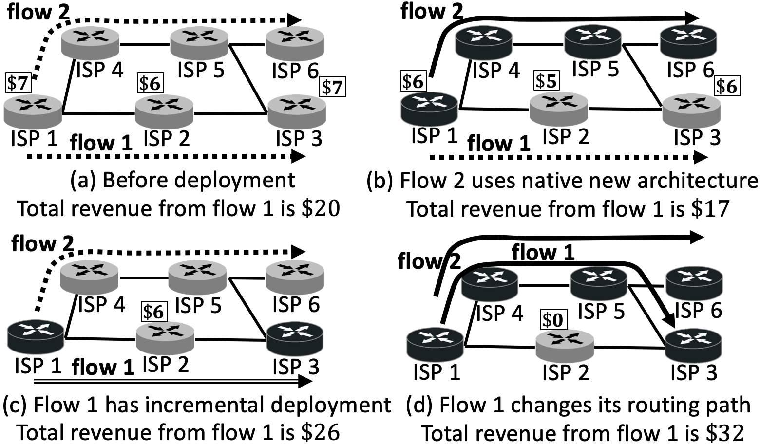
Figure 2: Example to deploy IPv6 (different deployment status)

II-B Model for The New Architecture

Given a set of $\mathcal{S}\subseteq\mathcal{I}$ ISPs that deploy a new architecture, we model how this deployment influences the routing of flows and the revenues of ISPs.

$\bullet$ The deployment of the new architecture. Let $c_{i}\in\mathbb{R}_{+}$ denote ISP $i$’s launching cost to deploy a new architecture. This cost captures the expense of procuring new hardware, upgrading software, and payment for engineers to manage the new infrastructure, etc. We model two types of deployment: (1) native new architecture; (2) incrementally deployed new architecture. First, however, we must define critical ISPs.

Definition 1 (Critical ISP).

Define $\mathcal{C}(\vec{p})$ to be the set of ISPs such that the native new architecture can be enabled on routing path $\vec{p}$ if and only if all ISPs in $\mathcal{C}(\vec{p})$ deploy the new architecture. We call an ISP $i\in\mathcal{C}(\vec{p})$ a critical ISP of $\vec{p}$.

Note that the critical ISP set $\mathcal{C}(\vec{p})$ depends on the new protocol or architecture. For example, consider the routing path $\vec{p}_{1}$ in Fig. 2. To enable native IPv6 on $\vec{p}_{1}$, the critical ISPs are $\mathcal{C}(\vec{p}_{1})=\{1,2,3\}$. On the other hand, to enable native TCP on $\vec{p}_{1}$, none of the ISPs are critical, i.e., $\mathcal{C}(\vec{p}_{1})=\emptyset$. The reason is that IPv6 requires “all” ISPs along a path to deploy, while TCP requires only the end devices (not the ISPs) to deploy it. For the ease of presentation, we consider one protocol/architecture at any time, unless otherwise stated explicitly. We next define the “full path participation”.

Definition 2 (Full path participation).

A new architecture requires full-path participation, if for any routing path $\vec{p}$, $\mathcal{C}(\vec{p})$ contains all ISPs in $\vec{p}$.

Thus, IPv6 needs full path participation while TCP does not.

Some architectures can be incrementally deployed, where a routing path $\vec{p}$ can (partially) enable the functionality of the new architecture even when only a proper subset of critical ISPs in $\mathcal{C}(\vec{p})$ participate. A real-world example is “IPv6 tunneling”, where encapsulation is used to carry IPv6 packets through islands of IPv4-only ISPs between ISPs that have deployed IPv6. Incremental deployment may introduce additional overhead to the network protocols and thus degrade the performance of the new architecture. With incremental deployment, performance of the new architecture may improve as more critical ISPs along a routing path deploy it.

$\bullet$ Change of routing path. Let $\mathcal{P}_{f}$ denote the ordered set of all alternative routing paths of flow $f$. The routing protocol determines $\mathcal{P}_{f}$ (independent of the new architecture), ordering the paths in $\mathcal{P}_{f}$ according to their priority. Note that $p_{f}\in\mathcal{P}_{f}$ and $p_{f}$ has the highest priority in $\mathcal{P}_{f}$. In practice, a Border Gateway Protocol (BGP) router typically records multiple paths to the same destination[cisco_bgp], and then chooses one with the highest priority according to ISPs’ routing policy configuration and the path length. In our model, if multiple routing paths in $\mathcal{P}_{f}$ can use the native new architecture, flow $f$ switches to the one among them with the highest priority. If none of the routing paths in $\mathcal{P}_{f}$ can use the new architecture, the routing path $\vec{p}_{f}$ is not changed. Here, we assume a flow changes its routing path only when the native architecture is available (or otherwise there is no incentive to change the routing path). E.g. in Fig. 2(d), flow $1$ can use the new architecture via the route $(1,4,5,3)$, thus flow $1$ switches to this route.

Given the set of deployed ISPs $\mathcal{S}$ and flow $f$’s alternative routing paths $\mathcal{P}_{f}$, we have a unique routing path for each flow $f$. Let $\vec{P}_{f}(\mathcal{S})$ denote the routing path of $f$ when ISPs in $\mathcal{S}$ deploy the new architecture. It satisfies $\vec{P}_{f}(\emptyset)=\vec{p}_{f}$. Let $\mathcal{F}^{old}(\mathcal{S})$ and $\mathcal{F}^{new}(\mathcal{S})$ denote the set of flows who use the old and new architecture respectively. Here, $\mathcal{F}^{new}(\mathcal{S})\cap\mathcal{F}^{old}(\mathcal{S})=\emptyset$, $\mathcal{F}^{new}(\mathcal{S})\cup\mathcal{F}^{old}(\mathcal{S})=\mathcal{F}$, and $\mathcal{F}^{old}(\emptyset)=\mathcal{F}$. The set of flows $\mathcal{F}^{new}(\mathcal{S})$ includes flows that use the native new architecture or incremental deployment mechanisms. We use $b_{i,f}(\mathcal{S})\in\{0,1\}$ to indicate whether ISP $i$ is bypassed in flow $f$, formally

$$b_{i,f}(\mathcal{S})=\left\{\begin{aligned} &1,&&\text{if $i\in\vec{p}_{f}$ and $i\notin\vec{P}_{f}(\mathcal{S})$},\\ &0,&&\text{otherwise}.\end{aligned}\right.$$

We use the example in Fig. 2 to illustrate our model. In Fig. 2(a), the routing path of flow $1$ is $\vec{P}_{1}(\emptyset){=}(1,2,3)$. In Fig. 2(b), only flow $1$ uses the old architecture and $\mathcal{F}^{old}(\{1,4,5,6\}){=}\{1\}$. Meanwhile, only flow $2$ uses the new architecture and $\mathcal{F}^{new}(\{1,4,5,6\}){=}\{2\}$. The possible routing paths for flow $1$ are $\mathcal{P}_{1}=\{(1,2,3),(1,4,5,3)\}$. In Fig. 2(d), flow $1$ has routing path $\vec{P}_{1}(\{1,3,4,5,6\})=(1,4,5,3)$. In flow $1$, ISP 2 is bypassed, so $b_{2,1}(\{1,3,4,5,6\})=1$.

$\bullet$ Change in revenue. We first model the revenue change at the flow-level. Let $\Delta_{f}(\mathcal{S})\in\mathbb{R}$ denote the revenue change on flow $f$ when ISPs in $\mathcal{S}$ deploy the new architecture, i.e., the revenue of flow $f$ changes from $\sum_{i\in\mathcal{I}}r_{i,f}$ to $\sum_{i\in\mathcal{I}}r_{i,f}+\Delta_{f}(\mathcal{S})$. We assume the revenue change satisfies $\Delta_{f}(\mathcal{S})\geq 0$ for all $f\in\mathcal{F}^{new}(\mathcal{S})$ and $\Delta_{f}(\mathcal{S})\leq 0$ for all $f\in\mathcal{F}^{old}(\mathcal{S})$. This captures the assumption that the new architecture is superior to the old architecture in terms of the revenue, and the revenue of flows that use the old architecture may drop due to competition from the new architecture. Consider the single (call it $f$) in Fig. 1. Before deployment, $r_{1,f}=r_{3,f}=7$, $r_{2,f}=6$. After deployment, $\Delta_{f}(\{1,2,3\})=\$12$. The following assumption further characterizes the revenue from a flow $f\in\mathcal{F}^{new}(\mathcal{S})$.

Assumption 1.

For each $f\in\mathcal{F}^{new}(\mathcal{S})$, $\Delta_{f}(\mathcal{S})$ satisfies:

1. $\Delta_{f}(\mathcal{S})\leq\Delta_{f}(\mathcal{T})$ if $\mathcal{S}\subset\mathcal{T}$,

2. $\Delta_{f}(\mathcal{S}){=}\Delta_{f}(\mathcal{T})$ if $n_{f}(\mathcal{S}){=}n_{f}(\mathcal{T})$ and $\vec{P}_{f}(\mathcal{S}){=}\vec{P}_{f}(\mathcal{T})$,

where $n_{f}(\mathcal{S}){\triangleq}|\mathcal{C}(\vec{P}_{f}(\mathcal{S}))\cap\mathcal{S}|$ denotes the number of critical ISPs in the routing path of $f$ that deploy the new architecture.

(This quantity will play an important role in later results.) Assumption 1 captures that: 1) The revenue from a flow is non-decreasing as more ISPs deploy the new architecture; and 2) The revenue generated from a flow is determined by the number of critical ISPs who deploy the new architecture.

Now we model the revenue change at the level of individual ISPs. Here we only focus on the ISPs who do not deploy the architecture, as they share the revenue according to the existing contracts (or peering agreement) on the old architecture. We will address ISPs that deploy the new architecture in Sec. II-C. Let $\delta_{i,f}(\mathcal{S})\in\mathbb{R}$ denote the revenue change of ISP $i\not\in\mathcal{S}$ on flow $f$. Namely, the revenue share of ISP $i\not\in\mathcal{S}$ from flow $f$ changes from $r_{i,f}$ to $r_{i,f}+\delta_{i,f}(\mathcal{S})$ when some other ISPs deploy the new architecture. The following proposition characterizes desirable properties of $\delta_{i,f}(\mathcal{S})$.

Proposition 1.

The revenue change $\delta_{i,f}(\mathcal{S})$ of $i{\not\in}\mathcal{S}$ satisfies:

1. For each $f\in\mathcal{F}^{old}(\mathcal{S})$:

   $$\textstyle i\in\vec{p}_{f}\Rightarrow\delta_{i,f}(\mathcal{S})\leq 0\text{ and }i\not\in\vec{p}_{f}\Rightarrow\delta_{i,f}(\mathcal{S})=0.$$

2. For each $f\in\mathcal{F}^{new}(\mathcal{S})$:

   $$\textstyle b_{i,f}(\mathcal{S}){=}1{\Rightarrow}\delta_{i,f}(\mathcal{S}){=}-r_{i,f}\text{ and }b_{i,f}(\mathcal{S}){=}0{\Rightarrow}\delta_{i,f}(\mathcal{S}){=}0.$$

Proposition 1 captures that ISPs that are in the routing path of a flow that uses the old architecture may have revenue losses (e.g. ISPs of flow 1 in Fig. 2(b)), while those not in the path do not have revenue loss from the flow. Furthermore, for a flow that uses the new architecture: when an ISP $i\not\in\mathcal{S}$ is bypassed by a flow, the ISP’s revenue share from that flow becomes 0 (e.g. ISP 2 in Fig. 2(d)); otherwise the ISP’s revenue is unchanged (e.g. ISP 2 in Fig. 2(c)).

II-C The ISP’s Decision Model

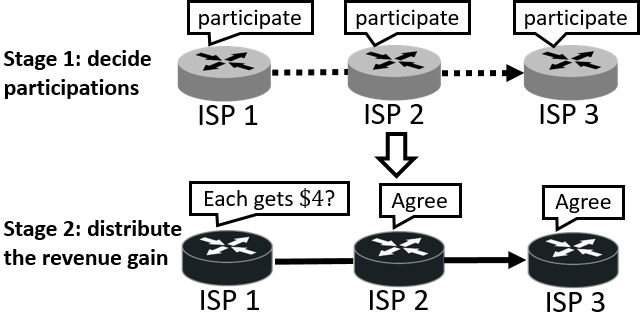
Figure 3: Two stages of ISPs’ game

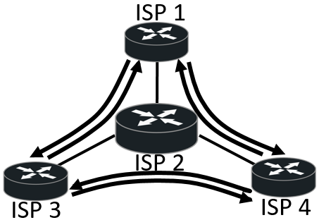
Figure 4: Example of flows, which imply multiple equilibria

We formulate a two-stage game as depicted in Fig. 4, where in the first stage, ISPs decide whether to deploy the new architecture and in the second stage, ISPs decide how to distribute the revenue. We will reason about the game via backward-induction, i.e. firstly analyze how ISPs distribute the revenue, and then analyze how ISPs decide whether to deploy.

$\bullet$ The second stage: distributing net revenue gain. We first focus on how the net revenue gain among ISPs in $\mathcal{S}$ will be distributed. We will describe a “proposal-agreement” process, for negotiating a distribution among the deploying ISPs, and we state an assumption (supermodularity) that ensures that a stable equilibrium exists, and can be computed a priori.

Let $v(\mathcal{S})$ denote the net revenue gain to ISPs $\mathcal{S}$. This is the total revenue increment of all ISPs, minus the revenue increment of all the non-deploying ISPs:

$$v(\mathcal{S})= \sum\nolimits_{f\in\mathcal{F}}\Delta_{f}(\mathcal{S})-\sum\nolimits_{i\not\in\mathcal{S}}\sum\nolimits_{f\in\mathcal{F}}\delta_{i,f}(\mathcal{S}).$$

As a simple consequence, if $v(\mathcal{I})<0$, it is impossible for all ISPs to deploy, as they will suffer revenue loss as a whole; thus we assume that $v(\mathcal{S}){\geq}0$. Moreover, we assume as follows:

Assumption 2 (supermodular).

For all $\mathcal{S}{\subseteq}\mathcal{T}$, $i{\in}\mathcal{I}$ and $i{\not\in}\mathcal{T}$:

$$v(\mathcal{S}\cup\{i\}){-}v(\mathcal{S})\leq v(\mathcal{T}\cup\{i\}){-}v(\mathcal{T}).$$

Assumption 2 states that the net revenue gain from one new ISP deploying the architecture cannot be smaller if a larger set of ISPs have deployed beforehand. That is, different ISPs are complementary in their effect on net revenue gain through deployment of the new architecture. Let $\phi(\mathcal{S},v){=}(\phi_{1},{\ldots},\phi_{|\mathcal{S}|}){\in}\mathbb{R}^{|\mathcal{S}|}$ denote a distribution mechanism for ISPs in $\mathcal{S}$, where $\phi_{i}(\mathcal{S}{,}v)$ is the net revenue gain distributed to ISP $i{\in}\mathcal{S}$ and $\sum_{i\in\mathcal{S}}\phi_{i}(\mathcal{S}{,}v){=}v(\mathcal{S})$.

We consider a “proposal-agreement” process described by Hart and Mas-Colell [hart1996bargaining] for ISPs to reach a fair distribution mechanism. It works in the following multi-round process. In each round there is a set of “active” players $\mathcal{T}{\subseteq}\mathcal{S}$, and a “proposer” $i\in\mathcal{T}$. In the first round, $\mathcal{T}{=}\mathcal{S}$. The proposer is chosen uniformly at random from $\mathcal{T}$. The proposer proposes a distribution mechanism $\phi^{\prime}$ that satisfies $\sum_{i\in\mathcal{T}}\phi_{i}^{\prime}(\mathcal{T},v)=v(\mathcal{S})$. If all members of $\mathcal{T}$ accept it, then each ISP in $\mathcal{T}$ will be distributed the revenue gain defined by $\phi_{i}^{\prime}(\mathcal{T},v)$. If the proposal is rejected by at least one member of $\mathcal{T}$, then we move to the next round, where with probability $\rho\geq 0$, the proposer $i$ drops out, and the set of active players becomes $\mathcal{T}\backslash\{i\}$. The dropped-out proposer $i$ gets a final distribution of $0$. This process models how ISPs bargain to get an acceptable (“fair”) distribution of revenue after the deployment. The bargaining power of an ISP comes from the ability to reject proposals it considers “unfair” and propose an alternative, and the risk of dropping out if the ISP proposes an unfair distribution.

Note that other processes, such as bargaining [gul1989bargaining] or bidding [perez2001bidding] can result in ISPs reaching the equilibrium whose existence is established in the next section.

$\bullet$ The first stage: the architecture deployment game. Given the mechanism $\phi$, how much revenue increment an ISP will share is determined by its own action (i.e., whether to deploy the architecture or not) and other ISPs’ actions. Thus, we formulate a strategic-form game to characterize ISPs’ strategic behavior in deciding whether to deploy the new architecture. We denote by $\tilde{\mathcal{C}}{\triangleq}\bigcup\nolimits_{{f}\in\mathcal{F}}\mathcal{C}(\vec{p}_{f})$ the set of all critical ISPs. If an ISP is not critical to any flow, it is irrelevant and will not get involved in the deployment. Hence the players of our interest are all the critical ISPs $\tilde{\mathcal{C}}$. Each ISP has two possible actions denoted by $\mathcal{A}{\triangleq}\{0,1\}$, where $1$ indicates that an ISP deploys the new architecture and $0$ indicates not. Let $a_{i}{\in}\mathcal{A}$ be the action of ISP $i{\in}\tilde{\mathcal{C}}$ and let $\bm{a}{\triangleq}(a_{i})_{i\in\tilde{\mathcal{C}}}$ denote the action profile of all critical ISPs. Given an action profile $\bm{a}$, the corresponding set of ISPs who deploy the new architecture is denoted by $\mathcal{S}_{\bm{a}}{\triangleq}\{i|a_{i}{=}1,i{\in}\tilde{\mathcal{C}}\}.$ The utility (or profit) $u_{i}(\bm{a})$ of ISP $i$ is the distributed revenue increment minus its launching cost, plus the change of revenue from the old architecture, i.e.

$$u_{i}(\bm{a})\triangleq\begin{cases}\phi_{i}(\mathcal{S}_{\bm{a}}{,}v){-}c_{i}&\text{if }a_{i}{=}1,\\ \sum_{f\in\mathcal{F}}\delta_{i,f}(\mathcal{S}_{\bm{a}})&\text{if }a_{i}{=}0,\end{cases}$$ (1)

where $c_{i}$ is ISP $i$’s cost in deploying the new architecture. We denote this “architecture deployment game” by a tuple $G{\triangleq}\langle{\tilde{\mathcal{C}},\mathcal{A},\bm{u}}\rangle$, where $\bm{u}{\triangleq}(u_{1},{\dots},u_{|\tilde{\mathcal{C}}|})$ is a vector of functions.

III Analyzing ISPs’ Decisions via Equilibrium

We first consider ISPs’ deployment decisions under a general setting, and show that multiple equilibria are possible in the architecture deployment game. We also derive a potential function to characterize the equilibria and show that when ISPs face uncertainty, the equilibrium that maximizes the potential function will be reached. Lastly, we study a special case to derive more closed-form results revealing more insights.

III-A Equilibrium of the Architecture Deployment Game

$\bullet$ Stable distribution mechanism in the second stage. In the following lemma, we apply the technique of Hart and Mas-Colell [hart1996bargaining] to prove the existence and uniqueness of a stable distribution mechanism for the proposal-agreement process defined in Sec. II-C, and derive a closed-form expression for the net revenue share for each ISP.

Lemma 1.

Under Assumption 2, the proposal-agreement process in Sec. II-C leads to a unique stationary subgame-perfect equilibrium, in which ISPs divide the net revenue gain as

$$\phi_{i}(\mathcal{S},v)=\varphi_{i}(\mathcal{S},\tilde{v})+\sum\nolimits_{f\in\mathcal{F}}\delta_{i,f}(\mathcal{S}\backslash\{i\}), \forall i\in\mathcal{S},$$ (2)

where $\varphi_{i}(\mathcal{S},\tilde{v})$ and $\tilde{v}(\mathcal{S})$ are defined as

$$\varphi_{i}(\mathcal{S},\tilde{v}){\triangleq}\!\sum_{\mathcal{T}\subseteq\mathcal{S}\setminus\{i\}}\!\!\!\!\frac{|\mathcal{T}|!(|\mathcal{S}|{-}|\mathcal{T}|{-}1)!}{|\mathcal{S}|!}[\tilde{v}(\mathcal{T}{\cup}\{i\}){-}\tilde{v}(\mathcal{T})],$$ (3)

$$\tilde{v}(\mathcal{S})\triangleq v(\mathcal{S})-\sum\nolimits_{i\in\mathcal{S}}\sum\nolimits_{f\in\mathcal{F}}\delta_{i,f}(\mathcal{S}\backslash\{i\}).$$ (4)

Definition 3.

The stable distribution mechanism is a distribution mechanism in the unique stationary subgame-perfect equilibrium of the game with the proposal-agreement process.

The physical meaning of this stationary subgame-perfect equilibrium is that no ISP in $\mathcal{S}$ can increase its net revenue gain share by proposing other distribution mechanisms or rejecting the stable distribution mechanism. For a mathematically rigorous definition of the stationary subgame-perfect equilibrium, we refer the reader to [hart1996bargaining]. ISPs may have other mechanisms to do non-cooperative bargaining, one can also apply other techniques [gul1989bargaining, Ma:2010:IEU] to show that they will reach the same stable distribution mechanism as in Lemma 1. In Lemma 1, the $\varphi_{i}(\mathcal{S},\tilde{v})$ derived in Eq. (3) is a Shapley value with a value function $\tilde{v}(\mathcal{S})$ defined in Eq. (4) instead of the net revenue $v(\mathcal{S})$. This is because $\tilde{v}(\mathcal{S})$ considers ISPs’ potential revenue loss from not participating in the proposal-agreement process.

$\bullet$ Deployment equilibria in the first stage. Based on the stable distribution mechanism in Lemma 1, we analyze ISPs’ deployment decisions via the notion of Nash equilibrium.

Definition 4.

An action profile $\bm{a}^{*}{\in}\mathcal{A}^{|\tilde{\mathcal{C}}|}$ is a strict pure Nash equilibrium of the game $G$, if for $\forall$ $i{\in}\tilde{\mathcal{C}}$, and $\forall a_{i}{\in}\mathcal{A}$, $a{\neq}\bm{a}^{*}_{i}$,

$$u_{i}(\bm{a}^{*})>u_{i}(\bm{a}^{*}_{[i:=a]}),$$

where the notation $\bm{a}_{[i:=x]}$ denotes the action profile $\bm{a}$ with $i$’s action $a_{i}$ replaced by $x$, i.e. $(a_{1},\ldots,a_{i-1},x,a_{i+1},\ldots,a_{|\tilde{\mathcal{C}}|})$.

In other words, at such equilibrium, no ISP can increase its utility by unilaterally deviating from its current action.

The game $G$ may have multiple equilibria. To illustrate, consider Fig. 4. Suppose that the launching cost of each ISP is $3. There are two equilibria. The first one is all ISPs do not deploy the new architecture. This is because an ISP’s unilateral deviation to deploy the new architecture will result in a loss of $\$3$. The second one is all ISPs deploy the new architecture. This is because all ISPs can have positive revenue gain when the new architecture is successfully deployed in the network.

We apply Topkis’s results[topkis2011supermodularity] to show that the game $G$ has a smallest (or largest) equilibrium with the smallest (or largest) set of deployed ISPs in our game in Lemma 2.

Lemma 2.

The set of equilibria of $G$ has a smallest element $\underline{\bm{a}}^{*}$, and a largest element $\overline{\bm{a}}^{*}$, such that $\underline{\bm{a}}^{\ast}\leq\bm{a}^{*}\leq\overline{\bm{a}}^{\ast}$ for any other equilibrium $\bm{a}^{*}$, where ordering is component-wise, or equivalently $\mathcal{S}_{\underline{\bm{a}}^{\ast}}{\subseteq}\mathcal{S}_{\bm{a}^{*}}{\subseteq}\mathcal{S}_{\overline{\bm{a}}^{\ast}}$.

Corollary 1.

(1) If $\forall iv(\{i\}){\leq}c_{i}$, then $(0,{\ldots},0)$ is an equilibrium. (2) If $\forall i$, $\varphi_{i}(\tilde{\mathcal{C}},\tilde{v}){\geq}c_{i}$, then $(1,\ldots,1)$ is an equilibrium.

Corollary 1 states that “all critical ISPs decide not to deploy” is an equilibrium, if no ISP’s revenue gain exceeds its launching cost when only that ISP deploys. Many architectures such as DiffServ and IPv6 satisfy this condition since their functionality can not be used under the deployment of a single ISP. Also, full deployment is an equilibrium if every critical ISP’s revenue gain is greater than its cost of deployment.

$\bullet$ Which equilibrium will be reached in the first stage? We apply two approaches to show that a unique equilibrium will be reached. The first one lets ISPs dynamically change their decisions in response to others’ actions. The second one lets ISPs reason about other ISPs’ actions. These two approaches reflect ISPs’ uncertainties on the benefits from deployment. In particular, before the deployment, ISP $i$ perceives a utility $u_{i}(\bm{a}){+}\varepsilon_{i}(\bm{a})$, where $\varepsilon_{i}(\bm{a})$ denotes the error or noise in the perception. When ISPs choose not to deploy the architecture (i.e. $a_{i}{=}0$), they are certain that there will be no revenue improvement, that is, $\varepsilon_{i}(\bm{a})=0$ when $a_{i}=0$. To facilitate analysis, we need the following lemma.

Lemma 3 ([monderer1996potential]).

If Eq. (3) holds, then $G$ is a potential game, i.e., $\exists$ a function $\Phi:\mathcal{A}^{|\mathcal{I}|}\mapsto\mathbb{R}$ such that for all $\bm{a}$ and $i$,

$$u_{i}(\bm{a}_{[i:=1]})-u_{i}(\bm{a}_{[i:=0]})=\Phi(\bm{a}_{[i:=1]})-\Phi(\bm{a}_{[i:=0]})$$ (5)

The above lemma states that the change of an ISP’s utility is equal to the change of a potential function. Therefore an ISP will have a positive profit to deploy an architecture if and only if her deployment increases the potential function. Therefore, there exists a one-to-one mapping between the equilibria of game $G$ and the local maxima of the potential function $\Phi$.

(1) Logit response dynamics. In this part, the error $\varepsilon_{i}(\bm{a})\in\mathbb{R}$ follows a logistic distribution with c.d.f. $\mathbb{P}[\varepsilon_{i}(\bm{a}){<}x]={1}/({1+e^{-x/\beta_{i}}})$ when $a_{i}{=}1$. When $a_{i}{=}0$, the error $\varepsilon_{i}(\bm{a})=0$ with probability 1. Here, the parameter $\beta_{i}{\geq}0$ represents ISP $i$’s degree of uncertainty. For example, when $\beta_{i}{\rightarrow}0$, $\varepsilon_{i}(\bm{a})$ is always close to $0$ which means that ISP $i$ has little uncertainty about its utility. We assume that an ISP will choose to deploy when its perceived utility of deploying is greater than the perceived utility of not deploying.

ISPs’ sequential dynamics are summarized in Algorithm 1. We divide time into slots, i.e., $t{\in}\{1,\ldots,T\}$. Let $\bm{a}^{(t)}$ denote the action profile at time slot $t$, and ISPs start with some initial action profile $\bm{a}^{(0)}$. At time slot $t$, we randomly pick one ISP, let’s say $i\in\tilde{\mathcal{C}}$, to make a decision based on ISPs’ actions in the last time slot $\bm{a}^{(t-1)}$. This setting captures that ISPs sequentially make decisions. More specifically, ISP $i$ chooses each action $a_{i}^{(t)}{\in}\{0,1\}$ with a probability that is logit-weighted by utility as shown in Line 4 of the Algorithm. The setting that ISPs can switch their decisions between “to deploy” and “not to deploy” captures that ISPs can buy (or rent) and sell (or stop renting) devices for the new architecture. Note that in the Logit Response Dynamics, we ignore the cost for an ISP to switch from one architecture to another.

1 ISPs have some initial action profile $\bm{a}^{(0)}$

2 for $t=1,\ldots,T$ do

3       Pick an ISP $i$ uniform randomly from all ISPs

4       choose ISP $i$’s action $a\in\{0,1\}$ with probability

$$\mathbb{P}[a_{i}^{(t)}=a|\bm{a}^{(t-1)}]=\frac{e^{u_{i}(\bm{a}_{[i:=a]}^{(t-1)})/\beta_{i}}}{e^{u_{i}(\bm{a}_{[i:=0]}^{(t-1)})/\beta_{i}}+e^{u_{i}(\bm{a}_{[i:=1]}^{(t-1)})/\beta_{i}}}.$$

Algorithm 1 Logit Response Dynamics

Lemma 4 ([alos2010logit][alos2017convergence]).

Following Algorithm 1, ISPs’ strategy profile converges to a unique (strict) equilibrium as the time $T{\rightarrow}\infty,\beta_{i}{\rightarrow}0,\forall i{\in}\mathcal{N}$. Given $\beta_{i}{=}\beta,\forall i{\in}\mathcal{N}$, as $T{\rightarrow}\infty$ the limiting distribution of ISPs’ action profiles is (if the limit exists)

$$\lim_{T\rightarrow\infty}\mathbb{P}(\bm{a}^{(T)}=\bm{a})\stackrel{{\scriptstyle\text{if exists}}}{{=}}e^{\Phi(\bm{a})/\beta}/\sum\nolimits_{\bm{a}\in\mathcal{A}^{|\tilde{\mathcal{C}}|}}e^{\Phi(\bm{a})/\beta}.$$ (6)

where $\Phi$ is the potential function of game $G$ defined in (5).

In the potential game $G$, ISPs are more likely to stay in the deployment status $\bm{a}$ with a higher potential value $\Phi(\bm{a})$. When ISPs’ uncertainties about the benefits of deployment vanishes, i.e. $\beta_{i}{\rightarrow}0$, ISPs’ dynamics lead to a unique equilibrium that maximizes the potential function, i.e. $\arg\max_{\bm{a}\in\mathcal{A}^{|\tilde{\mathcal{C}}|}}\Phi(\bm{a})$.

Algorithm 1 provides a dynamic model for a static game. We also introduce the following process for ISPs to reason about their decisions, which do not require ISPs’ dynamic plays.
(2) Iterative elimination of dominated strategies. Another perspective is that an ISP infers other ISPs’ behaviors. Before deployment, ISP $i$ perceives a revenue change $(1{+}\theta_{i})\Delta_{f}(\mathcal{S}_{\bm{a}})$ for the flow ${f}$. Then, we have $\varepsilon_{i}(\bm{a})\triangleq\theta_{i}\phi_{i}(v,\mathcal{S}_{\bm{a}}),$ where $\theta_{i}\in\mathbb{R}$ is a random variable that represents ISP $i$’s uncertainty towards the new architecture, and different $\theta_{i}^{\prime}s$ are independent. A negative (or positive) perception error $\varepsilon_{i}$ means ISP $i$ is pessimistic (or optimistic) about the new architecture. The perceived revenue change $(1+\theta_{i})\Delta_{f}(\mathcal{S}_{\bm{a}})$ is only known to ISP $i$, while the distribution of $\theta_{i}$ is known to all the ISPs. We denote the strategy of an ISP $i$ as a function from the uncertainty parameter $\theta_{i}$ to its action: $s_{i}(\theta_{i}):\mathbb{R}{\mapsto}\{0,1\}$. Since $\theta_{i}$ fully describes ISP $i$’s perceived utility, the strategy functions $s_{i}(\cdot)$ specify each ISP’s action facing different perceived utilities.

To investigate in ISPs’ strategies, we use the concept called iterative strict dominance [frankel2003complementarity]. The basic idea is that ISPs will not choose those actions which are known to have worse profit in expectation. For example, an ISP will not deploy IPv6 if it will lose money by deploying it. Due to page limits, we omit the detailed procedure of the iterative strict dominance [arXiv_version].

Lemma 5 ([frankel2003complementarity]).

Under Assumption 2, as $\theta_{i}$’s distribution concentrates around zero for each $i\in\mathcal{S}$, ISPs have a unique strategy profile after the iterative elimination of dominated strategies. Moreover, when the perception error $\theta_{i}\rightarrow 0$, ISPs have the unique actions $(s^{\ast}_{i}(0))_{i\in\tilde{\mathcal{C}}}{\in}\arg\max_{\bm{a}\in\mathcal{A}}\Phi(\bm{a})$.

This lemma states that under the iterative elimination of dominated strategies, the equilibrium that maximizes the potential function will be reached as the perception error diminishes.

Definition 5.

The “robust equilibrium” in our potential game $G$ is the equilibrium that maximizes the potential function.

Some economic experiments were carried out [heinemann2004experiments] that coincide with the prediction of “robust equilibrium”.

III-B A Case Study

We study a special case, under which we derive more closed-form results revealing more insights. In this particular case, the routing path is not allowed to change:

$$\mathcal{P}_{f}=\{\vec{p}_{f}\}, \forall f{\in}\mathcal{F},$$ (7)

and no revenue loss is caused by the competition between the old architecture and new architecture, i.e.,

$$\Delta_{f}(\mathcal{S})=0, \forall f{\in}\mathcal{F}^{old}(\mathcal{S}).$$ (8)

Note that Eq. (2) is NP-hard to solve, because the Shapley value is NP-hard to compute in general [deng1994complexity]. Using Eq. (7) and (8), we derive a simpler expression of Eq. (2) with computational complexity significantly reduced.

Theorem 1.

Suppose Eq. (7), Eq. (8) and Assumption 1 hold. Then, Eq. (2) can be simplified to

$$\phi_{i}(\mathcal{S},v){=}\sum\nolimits_{{f}\in\mathcal{F}}\mathbbm{1}_{\{i\in\mathcal{C}(\vec{p}_{f})\}}\frac{\Delta_{f}(\mathcal{S})}{n_{f}(\mathcal{S})},~{}\forall i{\in}\mathcal{S}.$$ (9)

where $\mathbbm{1}_{A}\in\{0,1\}$ is an indicator function for the event $A$.

Due to page limit, proofs are in the supplement. Recall that $n_{f}(\mathcal{S})$ is the number of critical ISPs of flow $f$ that deploy the new architecture. Eq. (9) in Theorem 1 states that the revenue gain of a flow ${f}$ is evenly distributed to all the $n_{f}(\mathcal{S})$ critical ISPs that deploy the new architecture, and the Shapley value of an ISP is the sum of such distributions from different flows.

To illustrate, let us consider Fig. 4, which depicts a network consisting of 4 ISPs and 6 flows where each flow passes through three ISPs. Suppose the new architecture requires a full-path participation and all four ISPs $\mathcal{S}{=}\{1,2,3,4\}$ upgrade to the new architecture. Each flow has a revenue gain of $3, i.e. ${\Delta_{f}(\mathcal{S}){=}\$3},\forall{f}{\in}\mathcal{F}$. According to (9), each ISP shares $3/3=$1 in each flow. In total, ISP 1, 3 and 4 gain $4 because they participate in 4 flows. One can see that ISP 2 shares a higher Shapley value of $6, because all 6 flows must go through it. In other words, ISP 2 has a higher contribution to the revenue gain of the new architecture. Based on Theorem 1 , we next derive a closed-form potential function for the game $G$.

Theorem 2.

Given the same conditions in Theorem 1, the potential function that satisfies Eq. (5) can be

$$\Phi(\bm{a})\triangleq\sum\nolimits_{{f}\in\mathcal{F}}\sum\nolimits_{m=1}^{n_{f}(\mathcal{S}_{\bm{a}})}\frac{{\tilde{\Delta}_{f}}(m)}{m}-\sum\nolimits_{i\in\tilde{\mathcal{C}}}a_{i}c_{i},$$ (10)

where $\tilde{\Delta}_{f}(m)$ is the value of $\Delta_{f}(\mathcal{S})$ when $n_{f}(\mathcal{S}){=}m$. We call $B(\mathcal{S}_{\bm{a}}){\triangleq}\sum\nolimits_{{f}{\in}\mathcal{F}}\sum\nolimits_{m=1}^{n_{f}(\mathcal{S}_{\bm{a}})}{\frac{\tilde{\Delta}_{f}(m)}{m}}$ the total immediate benefits.

This potential function $\Phi(\bm{a})$ has insightful physical meanings. The term $\tilde{\Delta}_{f}(m)/m$ is the revenue gain distributed to the $m^{th}$ deployer in flow ${f}$ immediately after the $m^{th}$ deployer’s deployment. The term $\sum_{m=1}^{n_{f}(\mathcal{S}_{\bm{a}})}{\tilde{\Delta}_{f}(m)}/{m}$ is all such immediate benefits that have been distributed to the past deployers in flow ${f}$. Summing over all flows, $B(\mathcal{S}_{\bm{a}})$ is the total immediate benefits that ISPs $\mathcal{S}_{\bm{a}}$ receive immediately when they deploy. Also, $\sum_{i\in\tilde{\mathcal{C}}}a_{i}c_{i}$ is the total launching costs of ISPs $\mathcal{S}_{\bm{a}}$. Therefore, the potential function $\Phi(\bm{a})$ is the total immediate benefits minus the total launching costs.

IV Deployability & Evolvability: Theoretical Analysis

Based on the equilibrium analysis in the last section, we first present general conditions on the deployability of a new architecture. We analyze the following four factors to reveal their impacts on the deployability: (1) the number of critical ISPs, (2) incremental deployment, (3) change of routing path, and (4) revenue loss from old functionalities.

IV-A General Conditions on Deployability

Definition 6.

An architecture is “deployable” (or “successfully deployed”) if all ISPs in $\tilde{\mathcal{C}}$ deploy in the robust equilibrium.

We next define a “profitable” architecture, whose benefit can cover the total launching cost of all critical ISPs $\tilde{\mathcal{C}}$.

Definition 7.

An architecture is profitable if

$$v(\tilde{\mathcal{C}})\geq\sum\nolimits_{i\in\tilde{\mathcal{C}}}c_{i}.$$ (11)

An architecture needs to be “profitable” to be successfully deployed. However, as we will derive in a more refined condition, some profitable architectures may not be deployed.

Corollary 2 (Necessary Condition for Deployment).

An architecture is successfully deployed only if the potential function satisfies $\Phi(\bm{1})\geq\Phi(\bm{0})$. Under conditions (7) and (8), this necessary condition has a closed-form expression:

$$B(\tilde{\mathcal{C}})\geq\sum\nolimits_{i\in\tilde{\mathcal{C}}}c_{i}$$ (12)

Condition (12) implies (11), but (11) does not imply (12).

Remark. This corollary comes from the requirement that $\Phi(\bm{1})$ should be the maximum value of the potential function, for “all critical ISPs to deploy” to be a robust equilibrium. It shows why a “profitable” architecture may not be successfully deployed. To illustrate, consider a network of three ISPs connected in a line topology. There is only one flow and all three ISPs are critical. Consider an architecture with a total benefit that is twice the total launching cost: $v(\tilde{\mathcal{C}}){=}2\sum_{i\in\tilde{\mathcal{C}}}c_{i}$. Then $B(\tilde{\mathcal{C}}){=}\frac{1}{3}v(\tilde{\mathcal{C}}){<}\sum_{i\in\mathcal{C}}c_{i}$, which violates condition (12) for successful deployment. Interestingly, even when the total benefit is twice the total launching cost, the new architecture still cannot be successfully deployed, because the total immediate benefits is less than the total launching cost.

Corollary 3 (Sufficient Condition for Deployment).

If condition $\Phi(\bm{1})\geq\Phi(\bm{0})$ holds, then in the robust equilibrium, a non-empty set of ISPs will deploy the new architecture.

This corollary states that condition $\Phi(\bm{1})\geq\Phi(\bm{0})$ is sufficient to guarantee that at least some of the ISPs (if not all) will deploy the new architecture. Together with Corollary 2, we could see that the condition (12) is both necessary and sufficient to determine whether an architecture is deployable.

IV-B Impact of The Number of Critical ISPs

We start our analysis with the simple setting of no incremental deployment mechanisms, i.e.,

$$\forall\mathcal{S}{\subseteq}\mathcal{I},f{\in}\mathcal{F}:\mathcal{C}(\vec{P}_{f}(\mathcal{S})){\setminus}\mathcal{S}{\neq}\emptyset\Rightarrow f{\in}\mathcal{F}^{old}(\mathcal{S}).$$ (13)

We also suppose conditions (7), (8) to hold (i.e., no change of routing path and no revenue loss by competitions between old and new architectures). Now, condition (12) is equivalent to

$${v(\tilde{\mathcal{C}})}/{\left(\sum\nolimits_{i\in\tilde{\mathcal{C}}}c_{i}\right)}\geq\gamma,$$ (14)

where $\gamma{\triangleq}v(\tilde{\mathcal{C}})/B(\tilde{\mathcal{C}})$ denotes the ratio between the total benefits $v(\tilde{\mathcal{C}})$ and the “total immediate benefits” $B(\tilde{\mathcal{C}})$. Condition (14) states that the ratio between the total benefit and total launching cost ${v(\tilde{\mathcal{C}})}/{\sum_{i\in\tilde{\mathcal{C}}}c_{i}}$ (“benefit-cost ratio” in short) should be higher than a “threshold” $\gamma$, for a new architecture to be deployable. As there is no incremental deployment mechanism (i.e. $\Delta_{f}(\mathcal{S}){=}0$ if $n_{f}(\mathcal{S}){<}|\mathcal{C}(\vec{p}_{f})|$), we have

$$\gamma=\frac{v(\tilde{\mathcal{C}})}{B(\tilde{\mathcal{C}})}=\frac{\sum_{{f}\in\mathcal{F}}{\Delta_{f}(\mathcal{C}(\vec{p}_{f}))}}{\sum_{f\in\mathcal{F}}\left({\Delta_{f}(\mathcal{C}(\vec{p}_{f}))}/{|\mathcal{C}(\vec{p}_{f})|}\right)}.$$ (15)

Eq. (15) comes from the facts that $v(\tilde{\mathcal{C}})=\sum_{{f}\in\mathcal{F}}{\Delta_{f}(\mathcal{C}(\vec{p}_{f}))}$ and $B(\tilde{\mathcal{C}}){=}\sum_{{f}\in\mathcal{F}}{\Delta_{f}(\mathcal{C}({\vec{p}_{f}}))}/{|\mathcal{C}(\vec{p}_{f})|}$. Eq. (15) states that $\gamma$ is the harmonic mean of the number of critical ISPs $|\mathcal{C}(\vec{p}_{f})|$ of the flows $f{\in}\mathcal{F}$, weighted by each flow’s maximum benefit $\Delta_{f}(\mathcal{C}(\vec{p}_{f}))$. Here, $|\mathcal{C}(\vec{p}_{f})|$ is the “degree of coordination” required by the new architecture for flow ${f}$. Then, the physical meaning of $\gamma$ is the “average degree of coordination” over the whole network. If an architecture requires a small number of critical ISPs to deploy for each flow, then $\gamma$ is small, and its deployability is high. Let us see some real-world cases.

Case 1: Deployment difficulty of DiffServ. To have QoS guarantees offered by DiffServ, all ISPs along the path are critical. Consider the network topology of a European education network GÉANT [uhlig2006providing]. If the revenue change is proportional to the weight, i.e., $\Delta_{f}(\mathcal{C}(\vec{p}_{f}))\propto w_{f}$ for each flow $f{\in}\mathcal{F}$, then the ratio $\gamma{=}3.3$ (more details are in Section VII). Hence, Eq. (14) states that only if the total benefits of DiffServ is higher than 3.3 times of its total launching cost, ISPs will deploy DiffServ in the GÉANT network. This high benefit-cost ratio make DiffServ difficult to be deployed. It provides an explanation why we see little adoption of DiffServ even if QoS guarantee is urgently needed in the current Internet.

Case 2: The Internet flattening phenomenon. We are witnessing a flattening Internet [Gill:2008:FIT, chiu2015we]. This happens as large content providers such as Google and Facebook place their data centers near end-users. Hence, the routing paths become shorter and many intermediate ISPs are bypassed. For many new architectures that require full-path participation (e.g. IPv6, DiffServ), the flattening Internet reduces the number of critical ISPs and makes these architectures more deployable. In fact, with co-located data centers, many Internet flows may traverse data centers within a single ISP (or the content provider). For those intra-data-center flows, one provider owns the entire topology, so there is only one critical node. Then $\gamma{=}1$ regardless of the revenue change; thus architectures like DiffServ can be deployed as soon as its total benefit exceeds its total launching cost. This explains why many proposed innovations for data centers are deployed.

IV-C Impact of Incremental Deployment Mechanism

Let us relax the settings of Sec. IV-B to allow incremental deployment mechanisms. Then, we can quantify the impact of incremental deployment mechanisms on $\gamma$ as follows:

$$\gamma{=}\frac{v(\tilde{\mathcal{C}})}{B(\tilde{\mathcal{C}})}{=}\frac{\sum_{{f}\in\mathcal{F}}{\Delta_{f}(\mathcal{C}(\vec{p}_{f}))}}{\sum_{{f}\in\mathcal{F}}\left(\frac{\Delta_{f}(\mathcal{C}(\vec{p}_{f}))}{|\mathcal{C}(\vec{p}_{f})|}+\sum_{m=1}^{|\mathcal{C}(\vec{p}_{f})|-1}\frac{\tilde{\Delta}_{f}(m)}{m}\right)}.$$ (16)

                                $\underbrace{\hskip 65.04034pt}_{\textbf{\small the term for incremental deployment}}$ The benefit from incremental deployment is reflected by $\tilde{\Delta}_{f}(m)$ in (16) where $m{\leq}|\mathcal{C}(\vec{p}_{f})|{-}1$. In contrast to (15), the incremental benefits brought by the mechanisms reduces the ratio $\gamma$, as the denominator in (16) becomes larger than that in (15). According to (14), we know incremental deployment mechanisms improve the deployability of an architecture, as illustrated in the following cases.

Case 3: Incremental deployment mechanisms of IPv6. Different incremental deployment mechanisms [mukerjee2013tradeoffs] enable IPv6 in the current Internet by selecting ingress/egress points to bypass the non-IPv6 areas. Despite many of these mechanisms, almost all the IPv6 traffic are using the native IPv6[ipv6_stat], which means these mechanisms are mostly not used. Based on this fact, we speculate that ISPs do not have significant revenue gain from these incremental mechanisms, i.e., $\tilde{\Delta}_{f}(m)$ is neglegible when $m{<}|\mathcal{C}(\vec{p}_{f})|$. Otherwise many ISPs would use these mechanisms to improve their revenue. Comparing (15) and (16), we see that incremental deployment mechanisms for IPv6 do not significantly reduce the value of $\gamma$, and thus do not increase the deployability of IPv6. In a word, these mechanisms for IPv6 failed because they did not provide significant incremental benefits to ISPs.

Case 4: XIA. XIA [han2012xia] is a future Internet architecture proposed recently that aims for an evolvable Internet. XIA has an intent-fallback system. If routers cannot operate on the primary “intent”, “fallbacks” will allow communicating parties to specify alternative actions. However, incremental benefits may be limited due to the characteristics of the intended functionality. For example, it is almost impossible to have QoS guaranteed without the participation of every ISP along the path. This means that $\tilde{\Delta}_{f}(m){=}0$ when $m{<}|\mathcal{C}(\vec{p}_{f})|$. Our model predicts that XIA has low deployability, because it is a network layer protocol and thus has a large number of critical ISPs. For example, XIA can be deployed in GÉANT network only if its total benefit is 3.3 times higher than its total launching cost, in the settings of Case 1. The problem is that the benefit for ISPs from deploying XIA is not clear.

IV-D Impact of Change of Routing Path

We relax the setting of Sec. IV-B to allow a flow to change its routing path during the deployment. First, we decompose ISPs’ net revenue gain $\tilde{v}(\mathcal{S})$ (defined in Lemma 1) into two components, $v_{g}$ and $v_{l}$, as follows:

$$\tilde{v}(\mathcal{S}){=}\overbrace{\sum_{f\in\mathcal{F}}\Delta_{f}(\mathcal{S})}^{v_{g}(\mathcal{S})}\overbrace{{-}\sum_{i\not\in\mathcal{S}}\sum_{f\in\mathcal{F}}\delta_{i,f}(\mathcal{S}){-}\sum_{i\in\mathcal{S}}\sum_{f\in\mathcal{F}}\delta_{i,f}(\mathcal{S}\backslash\{i\})}^{v_{l}(\mathcal{S})}.$$

Then, we can characterize the impact of change of routing path on the net revenue distribution in the following lemma.

Lemma 6.

The Shapley value $\varphi_{i}(\mathcal{S},\tilde{v})$ defined in Eq. (3) can be expressed as $\varphi_{i}(\mathcal{S},\tilde{v}){=}\varphi_{i}(\mathcal{S},v_{l}){+}\varphi_{i}(\mathcal{S},v_{g})$. If (8) and (13) hold, then $\varphi_{i}(\mathcal{S},v_{l})\geq 0$ and $\varphi_{i}(\mathcal{S},v_{g})$ satisfies

$$\varphi_{i}(\mathcal{S},v_{g}){=}\sum_{f\in\mathcal{F}}\sum_{\mathcal{P}\subseteq\mathcal{P}_{f}}\frac{(-1)^{|\mathcal{P}|-1}\Delta_{f}(\tilde{\mathcal{C}})}{|\bigcup_{\vec{p}\in\mathcal{P}}\mathcal{C}(\vec{p})|}\mathbbm{1}_{\left\{\begin{subarray}{c}i\in\bigcup_{\vec{p}\in\mathcal{P}}\mathcal{C}(\vec{p}),\\ \bigcup_{\vec{p}\in\mathcal{P}}\mathcal{C}(\vec{p})\subseteq\mathcal{S}\end{subarray}\right\}}.$$

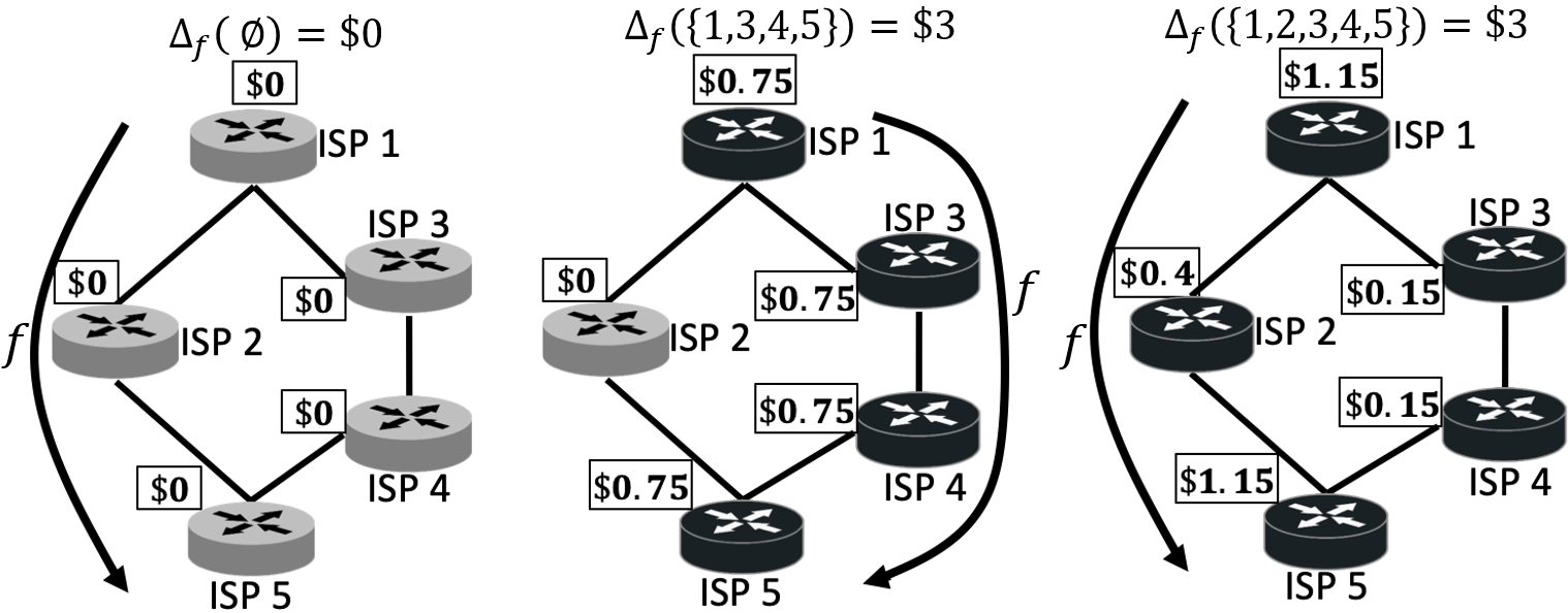
Figure 5: The routing path and ISPs’ $\varphi_{i}(\mathcal{S},v_{g})$ - before deployment (left), partial deployment (middle) and after deployment (right)

We use the Shapley value $\varphi(\mathcal{S},v_{g})$ in Lemma 6 to illustrate the impact of change of routing path. Consider Fig. 5 which depicts one flow $f$ and its two alternative routing paths $\mathcal{P}_{f}{=}\{(1,2,5),(1,3,4,5)\}$. All the ISPs along a path are critical to the new architecture. Before the deployment (left figure of Fig. 5), $\Delta_{f}(\emptyset){=}0$, so $\varphi_{i}(\mathcal{S},{v}_{g}){=}\$0$ for $1{\leq}i{\leq}5$. When ISPs $\mathcal{S}{=}\{1,3,4,5\}$ deploy the new architecture (middle figure of Fig. 5), the total revenue increment from the new architecture is $v_{g}(\mathcal{S}){=}\Delta_{f}(\mathcal{S}){=}\$3$. Then, each of these four ISPs has a net revenue share $\varphi_{i}(\mathcal{S},{v}_{g}){=}\$0.75$ for $i{=}1,3,4,5$. When all ISPs $\mathcal{I}{=}\{1,2,3,4,5\}$ deploy the new architecture (right figure of Fig. 5), the routing path of $f$ is (1,2,5). Then, ISP 1 has a Shapley value $\varphi_{1}(\mathcal{I},{v}_{g}){=}3{\times}(1{/}3{+}1{/}4{-}1{/}5){=}\$1.15$ according to Lemma 6. This is because ISP 1 is a critical ISP for both routing paths $(1,2,5)$ and $(1,3,4,5)$. Similarly, ISP 3 has a Shapley value $\varphi_{3}(\mathcal{I},v_{g}){=}3{\times}(1/4{-}1/5){=}\$0.15$. We observe that ISP 1 has a higher Shapley value than ISP 3. This is because ISP 1 is critical in more routing paths, thus it has a larger bargaining power to share the revenue gain.

Based on the Shapley value in Lemma 6, we have the following Theorem for the impact of change of routing paths.

Theorem 3.

If all conditions in Lemma 6 hold, then $\Phi(\bm{1})\geq\Phi(\bm{0})$ under $|\mathcal{P}_{f}|{=}1$ implies $\Phi(\bm{1})\geq\Phi(\bm{0})$ under $|\mathcal{P}_{f}|{\geq}1$.

Theorem 3 shows that the change of routing paths increases the deployability of a new architecture. This is because the change of routing paths will let the non-deploying ISPs be bypassed and lose revenue, thus, give them incentives to deploy.

IV-E Impact of Revenue Loss from Old Architecture

Let us relax the setting of Sec. IV-B to study the impact of revenue loss caused by the competition between the old and the new architectures. Recall that $w_{f}$ is the proportional traffic volume of flow $f$. We model the revenue change of a flow $f{\in}\mathcal{F}^{old}(\mathcal{S})$ that uses the old architecture as

$$\textstyle\Delta_{f}(\mathcal{S}){=}-\sigma|\vec{p}_{f}|w_{f}\sum_{h\in\mathcal{F}^{new}(\mathcal{S})}w_{h}, \forall f{\in}\mathcal{F}^{old}(\mathcal{S}).$$ (17)

Eq. (17) captures that the revenue loss of the old architecture is proportional to the total volume of flows that can use the new architecture, i.e., $\sum_{h{\in}\mathcal{F}^{new}}w_{h}$. Here, the parameter $\sigma{\geq}0$ captures the scale of revenue losses. An ISP $i{\not\in}\mathcal{S}$ that does not deploy the new architecture has the following revenue loss:

$$\delta_{i,f}(\mathcal{S}){=}\begin{cases}-\sigma w_{f}\sum_{h{\in}\mathcal{F}^{new}(\mathcal{S})}w_{h},&i{\in}\vec{p}_{f}\text{ and }f{\in}\mathcal{F}^{old}(\mathcal{S}),\\ 0,&\text{otherwise}.\end{cases}$$ (18)

Let $\bar{N}_{c}{\triangleq}({\sum_{f\in\mathcal{F}}w_{f}|\mathcal{C}(\vec{p}_{f})|^{2}})/({\sum_{h\in\mathcal{F}}w_{h}|\mathcal{C}(\vec{p}_{h})|})$ denote the weighted average number of critical ISPs over all flows in the network, where the weight for a flow $f$ is $w_{f}|\mathcal{C}(\vec{p}_{f})|$.

Theorem 4.

Suppose we have no change of routing path, i.e. (7), and no incremental deployment mechanisms, i.e. (13). Suppose the revenue loss of flows and ISPs satisfies (17) and (18). If $\sum_{f{\in}\mathcal{F}}w_{f}\mathbbm{1}_{\{i{\in}\vec{p}_{f}\}}\leq\sum_{f{\in}\mathcal{F}}{w_{f}|\mathcal{C}(\vec{p}_{f})|}/(|\mathcal{C}(\vec{p}_{f})|+\bar{N}_{c}+1)$ holds for all $i\in\tilde{\mathcal{C}}$, then $\Phi(\bm{1})\geq\Phi(\bm{0})$ under $\sigma=0$ implies $\Phi(\bm{1})\geq\Phi(\bm{0})$ under $\sigma>0$.

Theorem 4 states that when no ISP participates in more than a threshold volume of flows, ISPs’ revenue loss from old architecture will make the new architecture easier to deploy, rather than the other way around. Recall that $\bar{N}_{c}$ is the weighted average number of critical nodes in the flows, and $w_{f}$ is the weight of flow $f$. When all the flows have the same number of critical nodes $N_{c}$, the threshold fraction $\sum_{w\in\mathcal{F}}w_{f}{|\mathcal{C}(\vec{p}_{f})|}/(|\mathcal{C}(\vec{p}_{f})|{+}\bar{N}_{c}{+}1)=N_{c}/(2N_{c}{+}1)<0.5$.

Let us apply Theorem 4 to examine a real-world case. For GÉANT network, suppose the new architecture requires a “full-path participation”, then the threshold $\sum_{f{\in}\mathcal{F}}{w_{f}|\mathcal{C}(\vec{p}_{f})|}/(|\mathcal{C}(\vec{p}_{f})|{+}\bar{N}_{c}{+}1)$ is 0.407. Moreover, The condition that “no ISP participates to more than 40.7% of all flow volumes” holds for every ISP in GÉANT network. From Theorem 4, we know that for the GÉANT network, a new architecture is more deployable if we consider ISPs’ revenue loss from the old architecture.

V Extensions

Our results thus far consider binary actions, i.e., each ISP deploys the new architecture either in all of its networks, or in none of them. Moreover, we focus on one new architecture. Now, we extend our model to allow more than two actions and multiple competing new architectures respectively.

V-A Partial Deployment in Sub-networks

We first extend our previous binary action model, where $a_{i}{\in}\{0,1\}$, to allow more actions. We model that ISP $i$ has a finite set of devices denoted by $\mathcal{D}_{i}$, where an device could be a switch, router, etc. Each ISP can deploy the new architecture in a subset $\mathcal{A}_{i}\subseteq\mathcal{D}_{i}$ of its devices, and we use $\mathcal{A}_{i}$ to represent ISP $i$’s action. Namely, ISP $i$ has $2^{|\mathcal{D}_{i}|}$ possible actions. Fig. 7 illustrates this new action model. Note that no device belongs to multiple ISPs, so $\mathcal{D}_{i}{\cap}\mathcal{D}_{j}{=}\emptyset$ for any $i{\neq}j$. Let $\tilde{c}_{d}$ denote the cost to deploy the new architecture in device $d{\in}\bigcup_{i\in\mathcal{I}}\mathcal{D}_{i}$.

To simplify presentation, we assume that changes of routing path are not allowed and there is no competition among the old architecture and new architecture, i.e, conditions (7) and (8) hold. Note that dropping this assumption only involves a more complicated notation system. Let $\mathcal{D}_{i,f}\subseteq\mathcal{D}_{i}$ denote ISP $i$’s devices that support the routing path of flow $f$, i.e., $\vec{p}_{f}$. Without loss of generality, we assume that there are no dummy devices, i.e., $\bigcup_{f\in\mathcal{F}}\mathcal{D}_{i,f}=\mathcal{D}_{i}$. We say that an ISP $i$ deploys the new architecture for flow $f$ if it deploys this architecture in all of $\mathcal{D}_{i,f}$, i.e., $\mathcal{D}_{i,f}\subseteq\mathcal{A}_{i}$. Then, we define the set of critical ISPs that deploy the new architecture for flow $f$ as $\mathcal{S}_{f}(\bm{\mathcal{A}})\triangleq\{i|\mathcal{D}_{i,f}\subseteq\mathcal{A}_{i},i\in\tilde{\mathcal{C}}\},$ where $\bm{\mathcal{A}}\triangleq(\mathcal{A}_{i}:i\in\tilde{\mathcal{C}})$ denotes the action profile for all critical ISPs. To be consistent with Assumption 1, the revenue from a flow is determined by the number of critical ISPs that deploy the new architecture for this flow, i.e. $n_{f}(\mathcal{S}_{f}(\bm{\mathcal{A}}))$. We still use $\tilde{\Delta}_{f}(m)$ to denote the revenue increment of flow $f$ when $n_{f}(\mathcal{S}_{f}(\bm{\mathcal{A}}))=m$. Given action profile $\bm{\mathcal{A}}$, the revenue gain distributed to ISP $i\in\tilde{\mathcal{C}}$ is

$$\phi_{i}(\bm{\mathcal{A}},v){=}\sum_{{f}\in\mathcal{F}}\mathbbm{1}_{\{i\in\mathcal{C}(\vec{p}_{f}),\mathcal{D}_{i,f}\subseteq\mathcal{A}_{i}\}}\frac{\Delta_{f}(\mathcal{S}_{f}(\bm{\mathcal{A}}))}{n_{f}(\mathcal{S}_{f}(\bm{\mathcal{A}}))}.$$

Then, under action profile $\bm{\mathcal{A}}$, the utility of ISP $i$ is

$$u_{i}(\bm{\mathcal{A}})\triangleq\begin{cases}0,&\text{if }\mathcal{A}_{i}=\emptyset,\\ \phi_{i}(\bm{\mathcal{A}},v)-\sum_{d\in\mathcal{A}_{i}}\tilde{c}_{d},&\text{otherwise}.\end{cases}$$

Theorem 5.

Suppose (7) and (8) hold and ISPs’ total launching cost is a constant, i.e. $\sum_{i\in\tilde{\mathcal{C}}}c_{i}{=}\sum\nolimits_{i\in\tilde{\mathcal{C}}}\sum\nolimits_{d\in\mathcal{D}_{i}}\tilde{c}_{d}$. Then an architecture is “deployable” under the partial deployment action model, if and only if this architecture is “deployable” under the binary action model.

Theorem 5 states that whether ISPs can partially deploy a new architecture in sub-networks does not affect the architecture’s deployability. The reason is that the “degree of coordination” depends on the number of decision makers (i.e. the number of ISPs) in a flow, rather than the number of devices.

V-B Competing Architectures

We extend our model to study multiple competing architectures with similar functionalities. We will show that a more “deployable” architecture will have a competitive advantage.

$\bullet$ Deployment price of an architecture. ISPs charge customers for using the new functionality (e.g. CDN [azure_cdn], DDos protection [amazon_shield]). We consider a usage-based charging scheme. When all critical ISPs deploy the architecture, the unit price for the new functionality is $p{\in}\mathbb{R}_{+}$. Then, the revenue gain of a flow $f$ is $\Delta_{f}(\tilde{\mathcal{C}}){=}p{\times}w_{f},$ where we recall that $w_{f}$ is the proportional traffic volume of flow $f$. In comformance with our previous model, the unit price for flow $f$ when a subset $\mathcal{S}{\subset}\tilde{\mathcal{C}}$ of ISPs deploy is $p\Delta_{f}(\mathcal{S})/\Delta_{f}(\tilde{\mathcal{C}})$. We define the deployment price of an architecture (denoted by $p_{d}$) as the minimum unit price such that the condition (12) is satisfied. Namely, ISPs will deploy the architecture when the unit price is above $p_{d}$.

We illustrate the “deployment price” by considering the case in Sec. III-B where $\mathcal{P}_{f}=\{\vec{p}_{f}\}$ for each $f\in\mathcal{F}$ and $\Delta_{f}(\mathcal{S})=0$ for each $f\in\mathcal{F}^{old}(\mathcal{S})$. Then, according to Corollary 2, $p_{d}{\triangleq}\gamma\sum_{i\in\tilde{\mathcal{C}}}c_{i}/\sum_{f\in\mathcal{F}}w_{f}.$ Notice that the deployment price of an architecture depends on “degree of coordination” $\gamma$ (which depends on the number of critical ISPs) and the total launching cost $\sum_{i\in\tilde{\mathcal{C}}}c_{i}$.

$\bullet$ Multiple architectures under competition. Fig. 7 is an extension of the example in Fig. 2, where two architectures provide the same new functionality. Remember that architecture B requires all the ISPs 1,2,3 to deploy, and the launching cost for each ISP is $3. Architecture A, on the other hand, requires only ISP 4, the ISP closest to the end user, to deploy and has a launching cost $9 for that ISP. Note that the total launching costs for the two architectures are both $9. For simplicity, we again assume no incremental deployment mechanism and we have one unit usage volume. What will be a reasonable price for the new functionality? As we can see, only if the price of the new functionality is higher than the “deployment price” $27 will any ISP deploy B. Meanwhile, architecture A will be deployed as long as a price higher than $9 can be charged. Clearly a customer will not $27 if the same functionality is available for $9. Then, ISPs will choose architecture A, and architecture B will not be deployed because of the lower price reached by the more evolvable and competitive architecture A.

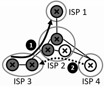
Figure 6: Partial Deployment in routers

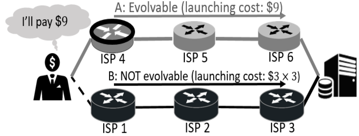
Figure 7: Competing architectures

Suppose we have $K$ new architectures providing the same functionality, with deployment prices $p_{d}^{(1)}{,}{\cdots},p_{d}^{(K)}$ respectively. We consider a market where ISPs are highly competitive so the customers can dictate the price. Here, we claim without rigorous proof that the customers will set the price to the lowest deployment price of these architectures, i.e. $\min_{k}\{p_{d}^{(k)}\}$. This is reasonable because the customers will not pay a higher price for a functionality if they could enjoy the same functionality with a lower price. Consequently, other architectures with higher deployment prices will not be successfully deployed. When competitive architectures have similar deployment price and total launching costs, the architecture with the lowest “degree of coordination” $\gamma$ will win. Let us apply these observations to study the following cases.

Case 5: IPv6 vs. NAT. IPv6 and NAT (Network Address Translation) both provide similar functionality of “addressing hosts”. In fact, NAT is now deployed in a great many ISPs, while IPv6 is still not deployed in many countries. In short, NAT wins and this observation could be explained by our model. IPv6 is a network-layer protocol which requires full-path participation. Although there are incremental deployment mechanisms, as we discussed before, they are rarely enabled by many ISPs. NAT is an application-layer solution that can be deployed transparently for most end users who need more addresses. The average AS path length is around 4 [path_lengths]. Therefore, IPv6 requires a much higher “degree of coordination” (around four times) compared to NAT.

Case 6: NDN vs. CDN. Content Delivery Network (CDN) caches data spatially close to end-users to provide high availability and better performance. Meanwhile, Named Data Networking (NDN) [ndn] is a future Internet architecture that names data instead of their locations. Their main functionalities are both to provide scalable content delivery. CDNs operate at the application-layer, so only the CDN owners need to deploy the CDN infrastructures. NDN is designed to operate as the network layer [ndn]; thus its deployment requires full-path participation, implying a degree of coordination around four (based on average AS path length). Suppose NDN has a comparable total launching cost as CDN. Then according to our model, NDN would have around four times higher deployment price than CDN. In order for NDN to overcome competition from CDN, it it would need to provide additional benefits and/or have incremental deployment mechanisms. Guided by our analysis, one possible incremental deployment mechanism would be to run NDN on top of IP as an overlay [jiang2014ncdn] to provide incremental benefits. This is possible since NDN is designed as a “universal overlay”, and could make NDN evolvable and competitive with CDN. Indeed, Cisco’s hybrid-ICN [hICN] pursues a related incremental deployment approach.

Case 7: Multipath TCP vs. Multipath QUIC. Multipath-TCP (MPTCP)[mptcp] is an extension of TCP, which enables inverse multiplexing of resources, and thus increases TCP throughput. MPTCP requires middleboxes (e.g., firewalls) in the Internet to upgrade so they do not drop its packets [mptcp_middlebox] because they do not recognize them. Therefore, the critical nodes for MPTCP include the senders, receivers, and the ISPs with middleboxes. In contrast, Multipath-QUIC (MPQUIC)[de2017multipath] is an extension of QUIC[langley2017quic] that achieves the multipath functionality of MPTCP. Because QUIC encrypts its packets and headers, MPQUIC avoids interference from middleboxes. Then the critical nodes of MPQUIC only include the senders and receivers. We argue that the total launching cost of MPQUIC is not more than that of MPTCP. This is because MPTCP and MPQUIC both require the senders and receivers to upgrade their software, but MPTCP additionally requires the middleboxes to be upgraded. Also, MPQUIC has lower degree of coordination. Comparing the total launching cost and the degree of coordination, our models predict that MPQUIC will be deployed more rapidly than (or instead of) MPTCP.

VI Mechanism Design to Enhance Deployability

Based on the observations thus far, we first design a coordination mechanism to enhance the deployability of a new architecture. Then, we improve the practicability of our mechanism via the idea of tipping set [heal2006supermodularity]. Here, we consider one new architecture, and do not allow partial deployment.

VI-A Coordination Mechanism Design

Recall that the difficulty of deployment comes from the requirement of coordination among decentralized ISPs. To mitigate this difficulty, we design a coordination mechanism. Before presenting our mechanism, we review some real-world examples to illustrate the power of coordination. From the historical data [ipv6_stat, ipv6_stat_ISOC] for the transition from IPv4 to IPv6, we observe that coordinating actions of are highly correlated with IPv6’s deployment. Before the first World IPv6 Launch Day organized by Internet Society in 2012 [world_ipv6_launch], less than 1% of users accessed their services over IPv6 [ipv6_stat]. In 2018, this number goes to nearly 25% [ISOC_dominant]. As another example, the Indian government produced a roadmap of IPv6’s deployment in July 2010 [india_gov] when the adoption rate was less than 0.5%. Now, over 30% of the traffic in India uses IPv6 [ipv6_stat]. In contrast, the government of China did not announce a plan to put IPv6 into large-scale use until Nov. 2017 [cn_government]. Now, less than 3% of traffics in China use IPv6 [ipv6_stat].

Formally, our coordination mechanism contains two steps:

1. Quoting: Each ISP $i\in\tilde{\mathcal{C}}$ submits a quote $q_{i}{\in}\mathbb{R}_{+}$ to the coordinator. An ISP’s quote is a contract under which the ISP would deploy the architecture once someone pays more than the quote. Quoting itself does not cost anything.

2. ISP selection: In this step, the coordinator selects a set of ISPs to deploy the architecture, and announces a reward for each of them. For each selected ISP, the announced reward is at least as high as that ISP’s quote. Then the selected ISPs deploy the new architecture, and the coordinator gives ISPs the announced reward.

The coordinator might be an international organization, group of governments, etc. In the second step of the mechanism, the coordinator selects the ISPs via the following optimization:

$$\text{maximize}_{\mathcal{S}\subseteq\tilde{\mathcal{C}}} |\mathcal{S}|,$$

subject to $$\varphi_{i}(\mathcal{S},\tilde{v})\geq q_{i},\forall i\in\mathcal{S},$$ (19)

where $\tilde{v}(\mathcal{S})$ is defined in Eq. (4). Let $\mathcal{S}^{*}(\bm{q})$ denote one optimal solution of the above optimization problem, where $\bm{q}\triangleq(q_{i}:i\in\tilde{\mathcal{C}})$. Finally, each selected ISP $i{\in}\mathcal{S}^{*}(\bm{q})$ gets a reward $\varphi_{i}(\mathcal{S}^{*}(\bm{q}),\tilde{v})$, which is at least as high as its quote.

ISPs may intentionally quote lower to increase the chance to be selected, or quote higher to ask for more reward. Our mechanism enforces ISPs to quote exactly their launching cost.

Theorem 6.

Suppose there is only one new architecture, ISPs have binary actions $\{0,1\}$ and Assumption 2 holds. Quoting $q_{i}{=}c_{i}$ is a weakly dominant strategy for each ISP $i{\in}\tilde{\mathcal{C}}$.

We further quantify the efficiency of our mechanism.

Theorem 7.

Under the same conditions as Theorem 6, if $\mathcal{S}\subset\mathcal{T}\implies v(\mathcal{S}){<}v(\mathcal{T})$ for any $\mathcal{S},\mathcal{T}$, the unique selection $\mathcal{S}^{*}(\bm{c})$ yields a maximal total revenue gain $v(\mathcal{S}^{*}(\bm{c}))$ for all ISPs.

Note that Theorem 6 and 7 still hold when we consider the change of routing path or the revenue loss from the old architecture, etc. The proof only requires that ISPs distribute the revenue gain via the “stable” distribution mechanism.

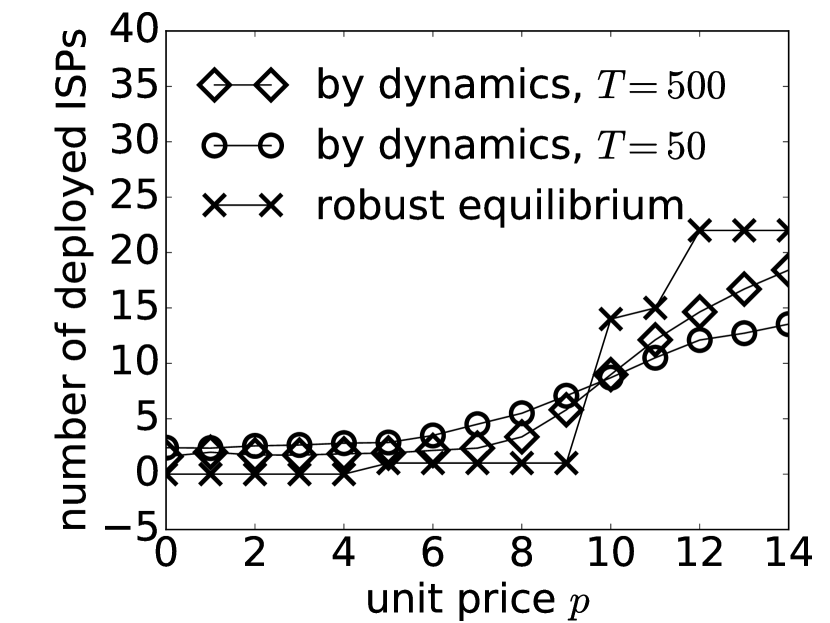
Figure 8: Logit-response dynamics (GÉANT)

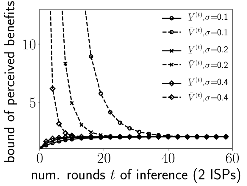
Figure 9: Two ISPs’ dynamics to infer their strategies

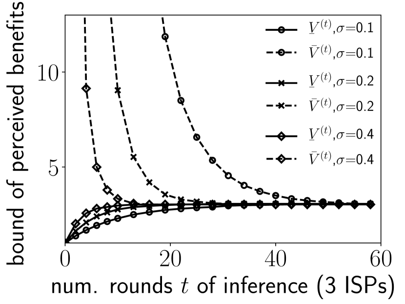
Figure 10: Three ISPs’ dynamics to infer their strategies

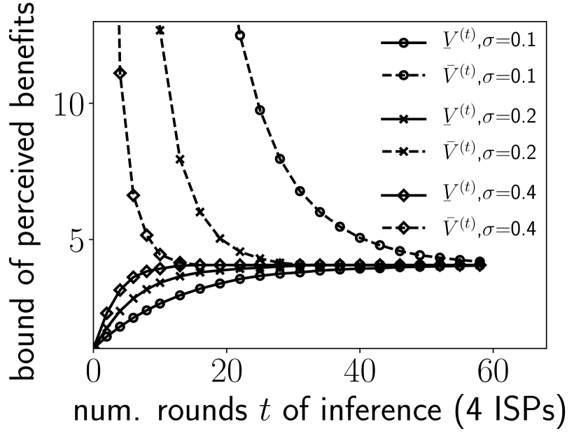
Figure 11: Four ISPs’ dynamics to infer their strategies

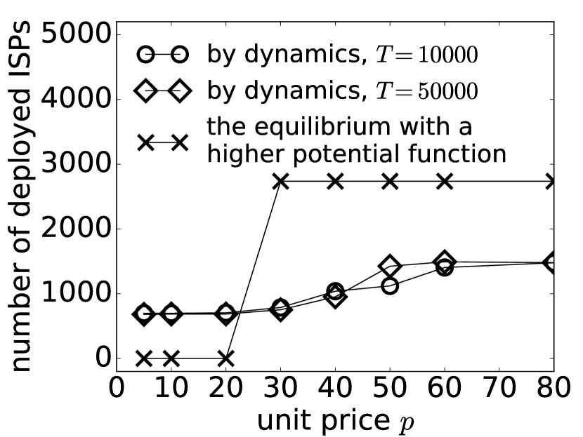
Figure 12: Logit-response dynamics (IPv4-net)

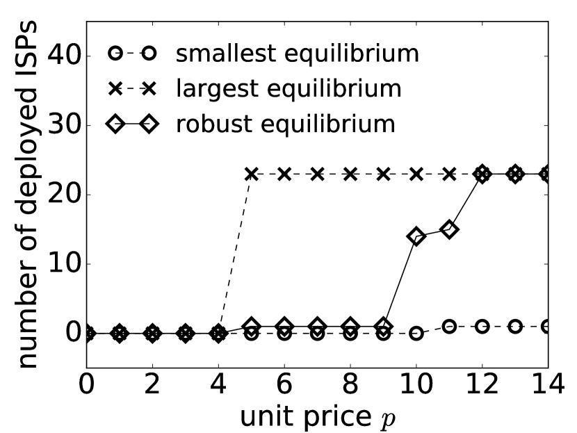
Figure 13: Unit price $p$ and the scale of equilibria (GÉANT)

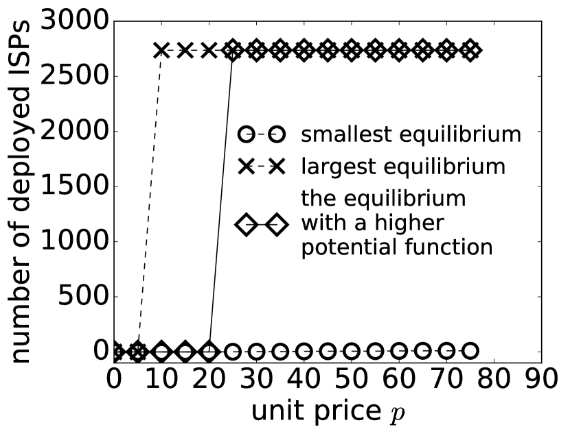
Figure 14: Unit price $p$ and the scale of equilibria (IPv4-net)

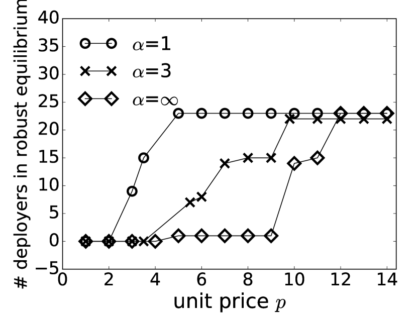
Figure 15: Incremental deployment mechanisms (GÉANT)

VII Numerical Experiments

VII-A Experiment Settings

Datasets. The first dataset [uhlig2006providing] was collected from a European education network GÉANT with 23 ASes (Autonomous System). The data contains a network topology $G{=}(\mathcal{I}{,}\mathcal{E})$ and a traffic matrix $\mathbf{T}{\in}\mathbb{R}^{I\times I}_{{\geq}0}$, where $T_{ij}$ records the traffic volume from the source node $i$ to the destination node $j$. There are $477$ flows of non-zero traffic volume in this dataset. The second dataset is the AS-level IPv4 topology collected by CAIDA in Dec. 2017 [caidatopology]. The dataset contains a weighted graph of 28,499 ASes $G{=}(\mathcal{I}{,}\mathcal{E})$, where each edge $(i{,}j){\in}\mathcal{E}$ can be either a direct or an indirect link from $i$ to $j$. This dataset does not contain the traffic matrix data. Thus, we synthesize a traffic matrix based on the Gravity method [roughan2005simplifying]. The idea is that the traffic volume from node $i$ to $j$ is proportional to the repulsive factor of the source node $i$ denoted by $T^{out}(i)$, and the attractive factor of the destination node $j$, denoted by $T^{in}(j)$, i.e. $T_{ij}{\propto}T^{out}(i){\times}T^{in}(j).$ We apply the Clauset-Newman-Moore method [clauset2004finding] to extract the largest cluster in the network. This cluster contains 2,774 nodes, and we take $T^{in}(i)$ and $T^{out}(j)$ to be i.i.d. exponential random variables with mean 1. From 2774$\times$2774 possible flows, we randomly select 74,424 (2%) as the flows with a positive demand of traffic for the new architecture.

Parameter settings. An ISP corresponds to an AS that has its own network policies, so we regard the ASes in the datasets as the ISPs in our model. It is known that GÉANT network uses IS-IS protocol [uhlig2006providing] that implements the Dijkstra shortest path algorithm. For flows with a positive traffic, let $\mathcal{F}{=}\{\text{traffics from $i$ to $j$}|i,j\!\in\!\mathcal{I},T_{i,j}\!>\!0\}$ be the set of flows, and $\vec{p}_{f}$ be the shortest path from the source to the destination for all flows $f\in\mathcal{F}$. As discussed in Section V-B, a new functionality such as CDN typically charges customers based on usage volume. Thus we assume that the revenue gain from a flow is proportional to the usage volume, i.e., $\Delta_{f}(\tilde{\mathcal{C}}){=}p{\times}w_{f}$, where $p$ is the unit price. Given a traffic matrix $\mathbf{T}$, the proportional traffic volume of a flow ${f}$ from source $s$ to destination $t$ is $w_{f}{\propto}T_{i,j}.$ Note that the launching cost of an ISP depends on the workload of the ISP. Therefore we assume that the launching cost of an ISP $i$ is proportional to the total amount of traffic through this ISP, i.e. $c_{i}{=}C{\times}\sum_{{f}\in\mathcal{F}}\bm{1}_{\{i\in\vec{p}_{f}\}}w_{f},$ where $C$ is the launching cost for a unit amount of traffic. For an architecture deployment game ${\langle}{{\tilde{\mathcal{C}}}{,}\mathcal{A}{,}\bm{u}}{\rangle}$, as we scale $p$ and $C$ linearly at the same rate, the utility function $\bm{u}$ scales linearly as well. Hence the Nash equilibria and the robust equilibrium will not be changed. Without loss of generality, we set $C{=}1$, and see the impact of $p$ (more generally, $p{/}C$).

Model settings. In our numerical experiments we consider fixed routing paths, no partial deployment and no revenue loss caused by the competition between the old and new architectures. This is because we focus on the reasons why a new architecture is difficult to deploy, and previously we have seen that other factors (change of routing path, partial deployment, and the competition between the old and new architectures) are generally not the major barriers to deployment.

VII-B Equilibrium of the Deployment Game

Logit-response dynamics of ISPs. We simulate ISPs’ behaviors by the logit-response dynamics defined in Sec. III, where we randomly initiate an ISP to deploy with probability 0.5. For the GÉANT network, we set $\beta_{t}{=}8{\times}10^{-5}{/}t$, and take the average of 200 runs. As shown in Fig. 11, the number of deployed ISPs is close to the predictions of the robust equilibrium. When $T{=}50$, each ISP on the average makes two decisions, and the outcome of dynamics is very close to the robust equilibrium. As we increase $T{=}500$, the outcome becomes closer to the robust equilibrium. Similar results are observed for the IPv4 network in Fig. 15. The logit-response dynamics lead to the “robust” equilibrium, as if ISPs are maximizing some potential function in the deployment.

ISPs’ inferring process to eliminate dominated strategies. Recall that ISPs eliminate the dominated strategies according to the process in our Sec. III. After the $t^{th}$ round of inference, it requires the perceived benefit to be at least $\underaccent{\bar}{V}^{(t)}{\triangleq}(1{+}\underaccent{\bar}{\theta}^{(t)})\Delta_{f}(\mathcal{I})$ for an ISP to decide to adopt, where $\underaccent{\bar}{\theta}^{(t)}$ is the lower bound of the estimated parameter $\theta$ after the $t^{th}$ round. Similarly, the upper bound of perceived benefit is $\bar{V}^{(t)}{\triangleq}(1{-}\bar{\theta}^{(t)})\Delta_{f}(\mathcal{I})$ for an ISP to decide not to adopt, where $\bar{\theta}^{(t)}$ is the upper bound of the estimation of $\theta$. It means that an ISP will definitely not adopt when the perceived benefit is below $(1+\underaccent{\bar}{\theta}^{(t)})\Delta_{f}(\mathcal{I})$, and an ISP will definitely adopt when the perceived benefit is above $(1+\bar{\theta}^{(t)})\Delta_{f}(\mathcal{I})$. When the perceived benefit is between $(1+\underaccent{\bar}{\theta}^{(t)})\Delta_{f}(\mathcal{I})$ and $(1+\bar{\theta}^{(t)})\Delta_{f}(\mathcal{I})$, an ISP is uncertain about its decision.

Consider a line-graph of $I$ ISPs ($I=2,3,4$) and one flow $f$. Each ISP has a launching cost of $c=1/I$, and there is no incremental deployment for this new architecture. Note that in this setting, all the ISPs are symmetric and have symmetric strategies. Fig. 11, Fig. 11 and 11 show the induction dynamics of firms. One can observe that ISPs become more certain about their decisions as the number of rounds $t$ increases. When the number of induction rounds exceeds 60, there is a threshold of perceived benefits for an ISP to decide whether to deploy the new architecture. When the number of ISPs increases, the threshold of perceived benefits increases. This complements our theoretical results for $\sigma\rightarrow 0$. One can see that an architecture is less deployable when there are more critical ISPs along the paths. Moreover, when the uncertainty $\sigma$ is larger, it requires fewer inference rounds to converge. This is because ISPs’ inferring process eliminates what they will not do, and with more uncertainty, ISPs will more quickly find what they will not do. We need to point out that realistic ISPs may not do inferences for a large number of rounds.

Lessons learned. The numerical results further validates our theoretical characterizations on the equilibrium of ISPs.

VII-C Quantifying the Deployability

Benefit-cost ratio. The unit price $p$ determines the benefit-cost ratio of the new architecture. For GÉANT network, the total benefit will be more than the total launching cost when $p{>}3.3$. Fig. 15 shows the impact of $p$ on the deployability without any incremental deployment mechanism. When $p{\leq}4$, there is only one equilibrium, namely “no ISP will deploy”, because the benefit of the new architecture is not enough to cover ISPs’ launching cost. When $p{\geq}5$, the largest equilibrium (with the largest set of deployers) is “all 23 ISPs deploy”. However, in the robust equilibrium, no more than one ISP will deploy until $p{\geq}10$. This is because the largest equilibrium will not have a positive potential function unless $p{\geq}9.54$. For the IPv4 network with 2,774 ISPs, computing the robust equilibrium is intractable, so in Fig. 15, Fig. 17, we choose one of the smallest/largest equilibria with a higher potential function which is the one that is possible to be the robust equilibrium. For the IPv4 network, a new architecture will be profitable when $p{\geq}4.78$. But only when $p{\geq}21.88$, the condition (9) for successful deployment can be satisfied. Hence, as seen from Fig. 15, only when $p{\geq}25$, “all ISPs to deploy” is the one that is possible to be a robust equilibrium. Similar phenomena are observed in both networks.

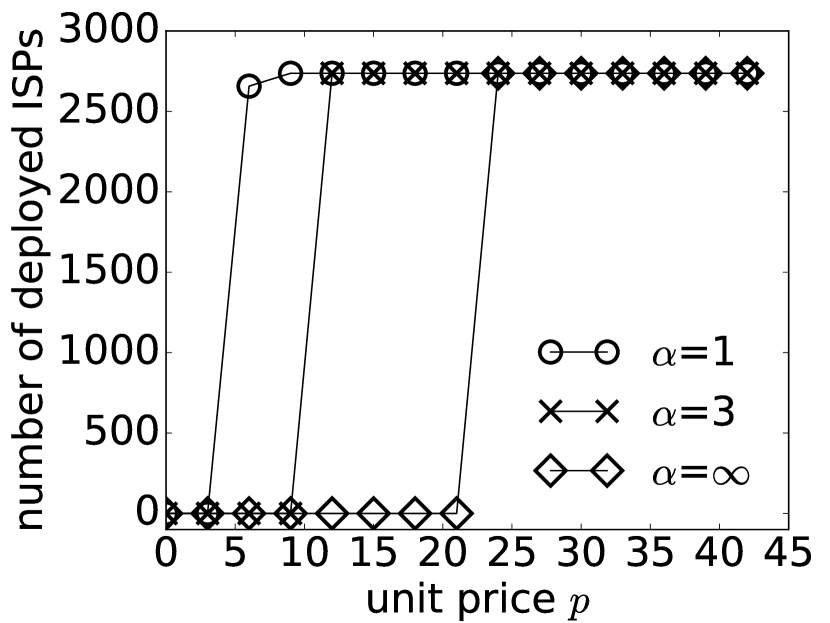
Figure 16: Incremental deployment mechanisms (IPv4-net)

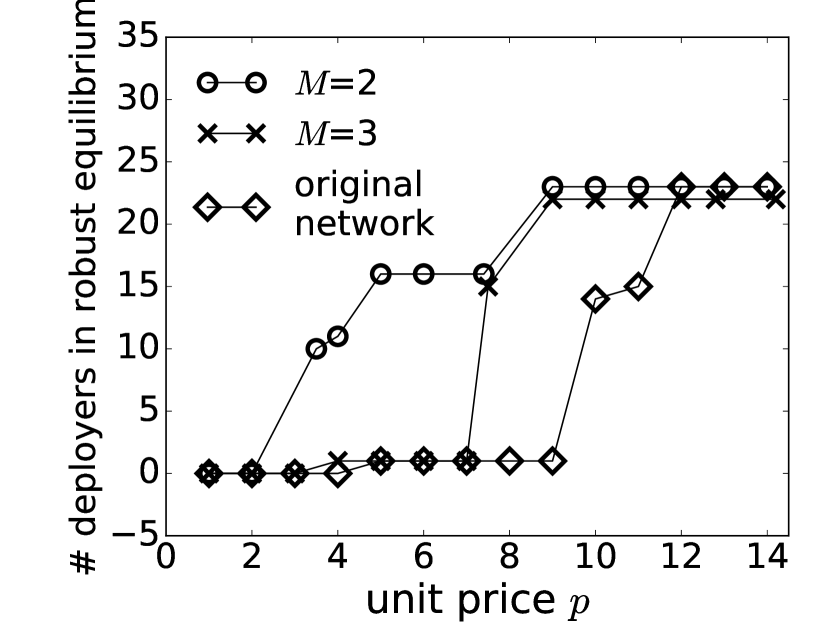
Figure 17: Impact of the flattening of network (GÉANT)

Incremental deployment mechanisms. We set the incremental benefit for flow ${f}$ as $\Delta_{f}(\mathcal{S}){=}\left({n_{f}(\mathcal{S})}/{|\mathcal{C}(\vec{p}_{f})|}\right)^{\alpha}pw_{f}$, when a set $\mathcal{S}{\subseteq}\tilde{\mathcal{C}}$ of ISPs deploy. The parameter $\alpha{\geq}1$ represents performances of incremental deployment mechanisms, where a smaller $\alpha$ indicates better performances. When $\alpha{=}{+}\infty$, there is no incremental benefit. In this case, as depicted in Fig. 15, the new architecture will not be deployed in the GÉANT network until $p{\geq}10$. In contrast, when $\alpha{=}1$, the architecture will be immediately deployed by 7 ISPs when $p{=}3$ and will be fully deployed by all ISPs when $p{\geq}5$. As $\alpha$ decreases, the new architecture gets deployed by more ISPs for a fixed $p$, in help of better incremental mechanisms. As seen in Fig. 17, better incremental mechanisms also improve the deployability of new architectures in the IPv4 network.

Internet flattening phenomenon. To see the impact of a flattening Internet, we shrink the paths of the original flows to have a maximum length of $M$. For a original flow $(i{,}v_{1}{,}{\ldots}{,}v_{L}{,}j)$ with a path length $L{+}2{>}M$, the flattened flow will be $(i{,}v_{L{-}M{+}3}{,}{\ldots}{,}v_{L}{,}j)$ that contains $i,j$ and $M{-}2$ ISPs which are nearest the destination $j$. This setting emulates that the sender uses data centers near the receiver. For GÉANT, Fig. 17 shows that when the maximum path length is shortened to $M{=}2$ (i.e. only the sender & receiver are in the flow), more than 10 ISPs will deploy when $p{\geq}3.5$. Meanwhile, in the original network, ISPs will deploy the new architecture only when $p{\geq}10$. Generally, the new architecture will be deployed by more ISPs in a more flattened network for a fixed $p$. One may observe that when content providers use data centers which are close to end users, they can pay a lower unit price $p$ to the ISPs so to enjoy the deployed new architectures/technologies.

Lessons learned. A profitable new architecture may not be deployed. Also (and unsurprisingly), higher benefit-cost ratio means higher deployability. The enhancement of incremental deployment mechanisms and the flattening Internet both improve the deployability of the new architectures.

We also conduct experiments to show the benefits of our coordination mechanism in Section VI. Please refer to the supplementary material or our technical report[arXiv_version] for details.

VIII Related Works

Designing future Internet architecture has been on the agenda since the early ages of the Internet [shenker1995fundamental]. A variety of future architectures were proposed [diff_serv, ndn, mobilityfirst, xia] to improve IPv4. Unfortunately, most of these proposals fail to deploy at scale. To make the Internet architectures evolvable, incremental deployment mechanisms are developed to enable universal access of IPv6 [gilligan2005basic, despres2010ipv6, mukerjee2013tradeoffs]. While an evolvable new architecture should be compatible with old architectures, our work shows via economic models that an evolvable architecture should also provide incremental “benefits” to ISPs. Internet flattening phenomenon was studied in paper [Gill:2008:FIT, chiu2015we], and our work formalizes their observations. A recent work [kirilin2018protocol] studied the incremental deployment of routing protocols, and suggested a coordinated adoption of a large number of ISPs.

Economics issues with the future Internet architectures have also been noticed. Wolf et al. developed ChoiceNet [Wolf:2014:CTE] to provide an economics plane to the Internet and a clear economics incentive for ISPs. Our work also points out that a new architecture may not be deployed even if it could be profitable for all ISPs. Along this direction, Ratnasamy et al. [Ratnasamy:2005:TEI] has a similar “chicken-and-egg” argument. Our economics analysis strengthens these arguments and quantitatively analyze the difficulty of coordination among decentralized ISPs. Some works studied the adoptability of BGP security protocols [Chan:2006:MAS, Gill:2011:LMD]. They conduct simulations, while we provide game-theoretic analysis to reveal key factors for the deployability, e.g. the coordination of ISPs. How to select some seeding ISPs to stimulate the deployment was studied [Goldberg:2013:DNT], but the incentives for the seeding ISPs remain a problem. Our economic mechanism considers the launching cost of the ISPs and requires the coordinator to invest nothing.

The “coordination failure” phenomenon was also studied in economics [cooper1988coordinating]. Monderer et al. [monderer1996potential] found that the equilibrium that maximizes a potential function accurately predicts Huyck’s experiments [van1990tacit]. Then Morris et al. [morris2001global] give reasons via the “global game”, which is used in our analysis.

IX Conclusion

This paper studies the deployability & evolvability of new architectures/protocols from an economic perspective. Our economic model shows that: (1) Due to coordination difficulty, being profitable is not sufficient to guarantee a new architecture to be widely deployed; (2) A superior architecture may lose to another competing architecture which requires less coordination. Our model explains why IPv4 is hard to be replaced, why IPv6, DiffServ, CDN have different deployment difficulties, and why we observe the “Internet flattening phenomenon”. Our model suggests that by changing the routing path, a new architecture becomes easier to deploy. In addition, the new architecture will be more deployable when the competition from the new architecture cause the revenue from the old functionality to decline, provided that each ISP participates in a small fraction of traffic volumes in the network. Our model also quantifies the importance of incremental deployment mechanisms for the deployment of new Internet architectures. For architectures like DiffServ with which incremental deployment mechanisms are not available, people may consider a centralized mechanism to help the deployment. The designers of new architectures like NDN and XIA can also use our model to evaluate and improve the deployability of their design. Our model predicts that the current design of NDN and XIA are difficult to deploy, and MPQUIC will win over MPTCP.

Li Ye received the B.Eng. degree from the School of Computer Science and Technology, University of Science and Technology of China, in 2016. He is currently a Ph.D student in the Department of Computer Science and Engineering, The Chinese University of Hong Kong, under the supervision of Prof. John. C.S. Lui. His research interests include network economics, data driven decision, and stochastic modeling. He is a member of the IEEE.

Hong Xie received the B.Eng. degree from the School of Computer Science and Technology, University of Science and Technology of China, in 2010, and the Ph.D degree from the Department of Computer Science and Engineering, The Chinese University of Hong Kong, in 2015, under the supervision of Prof. John. C.S. Lui. He is currently a Professor in the College of Computer Science, Chongqing University. His research interests include online learning algorithm and applications. He is a member of the IEEE.

John C.S. Lui received the Ph.D degree in computer science from the University of California at Los Angeles. He is currently the Choh-Ming Li Chair Professor with the Department of Computer Science and Engineering, The Chinese University of Hong Kong. His current research interests include Machine learning, online learning (e.g., multi-armed bandit, reinforcement learning), Network Science, Future Internet Architectures and Protocols, Network Economics, Network/System Security, Large Scale Storage Systems. He is an elected member of the IFIP WG 7.3, Fellow of ACM, Fellow of IEEE, Senior Research Fellow of the Croucher Foundation and was the past chair of the ACM SIGMETRICS (2011-2015). He received various departmental teaching awards and the CUHK Vice-Chancellor’s Exemplary Teaching Award. John is a co-recipient of the best paper award in the IFIP WG 7.3 Performance 2005, IEEE/IFIP NOMS 2006, SIMPLEX 2013, and ACM RecSys 2017.

Kenneth L. Calvert is Gartner Group Professor in Network Engineering at the University of Kentucky. His research deals with the design and implementation of advanced network protocols and services. He has been an associate editor of IEEE/ACM Transactions on Networking, a faculty member at Georgia Tech, and a Member of Technical Staff at Bell Telephone Laboratories in Holmdel, NJ. During 2016-2019 he served as Division Director for Computer and Network Systems in the Computer and Information Science and Engineering Directorate at the National Science Foundation of the US. He holds degrees from MIT, Stanford, and the University of Texas at Austin.

See pages - of supplement.pdf

References

- [1] Google, “Ipv6 stat.” www.google.com/intl/en/ipv6/statistics.html, 2018.
- [2] “Diffserv–the scalable end-to-end qos model,” Cisco, Tech. Rep., 2005.
- [3] Cisco, “Cisco report of cdn,” www.cisco.com/c/en/us/solutions/collateral/service-provider/visual-networking-index-vni/complete-white-paper-c11-481360.html, 2017.
- [4] NDN, “Named data networking project.” named-data.net.
- [5] XIA, “expressive internet architecture project,” www.cs.cmu.edu/~xia.
- [6] MobilityFirst, “Mobilityfirst future internet architecture project.” mobilityfirst.winlab.rutgers.edu.
- [7] CISCO, “Bgp best path selection algorithm,” www.cisco.com/c/en/us/support/docs/ip/border-gateway-protocol-bgp/13753-25.html.
- [8] S. Hart and A. Mas-Colell, “Bargaining and value,” Econometrica: Journal of the Econometric Society, pp. 357–380, 1996.
- [9] F. Gul, “Bargaining foundations of shapley value,” Econometrica: Journal of the Econometric Society, pp. 81–95, 1989.
- [10] D. Pérez-Castrillo and D. Wettstein, “Bidding for the surplus: a non-cooperative approach to the shapley value,” Journal of Economic Theory, vol. 100, no. 2, pp. 274–294, 2001.
- [11] R. T. B. Ma, D. M. Chiu, J. C. S. Lui, V. Misra, and D. Rubenstein, “Internet economics: The use of shapley value for isp settlement,” IEEE/ACM TON, vol. 18, no. 3, pp. 775–787, 2010.
- [12] D. M. Topkis, Supermodularity and complementarity. Princeton university press, 2011.
- [13] D. Monderer and L. S. Shapley, “Potential games,” Games and economic behavior, vol. 14, no. 1, pp. 124–143, 1996.
- [14] C. Alós-Ferrer and N. Netzer, “The logit-response dynamics,” Games and Economic Behavior, vol. 68, no. 2, pp. 413–427, 2010.
- [15] ——, “On the convergence of logit-response to (strict) nash equilibria,” Economic Theory Bulletin, vol. 5, no. 1, pp. 1–8, 2017.
- [16] D. M. Frankel, S. Morris, and A. Pauzner, “Equilibrium selection in global games with strategic complementarities,” Journal of Economic Theory, vol. 108, no. 1, pp. 1–44, 2003.
- [17] F. Heinemann, R. Nagel, and P. Ockenfels, “The theory of global games on test: experimental analysis of coordination games with public and private information,” Econometrica, vol. 72, no. 5, pp. 1583–1599, 2004.
- [18] X. Deng and C. H. Papadimitriou, “On the complexity of cooperative solution concepts,” Mathematics of Operations Research, vol. 19, no. 2, pp. 257–266, 1994.
- [19] S. Uhlig, B. Quoitin, J. Lepropre, and S. Balon, “Providing public intradomain traffic matrices to the research community (https://totem.info.ucl.ac.be/dataset.html),” ACM SIGCOMM Computer Communication Review, vol. 36, no. 1, pp. 83–86, 2006.
- [20] P. Gill, M. Arlitt, Z. Li, and A. Mahanti, “The flattening internet topology: Natural evolution, unsightly barnacles or contrived collapse?” in PAM ’08. Springer-Verlag, 2008.
- [21] Y.-C. Chiu, B. Schlinker, A. B. Radhakrishnan, E. Katz-Bassett, and R. Govindan, “Are we one hop away from a better internet?” in IMC ’15. ACM, 2015.
- [22] M. K. Mukerjee, D. Han, S. Seshan, and P. Steenkiste, “Understanding tradeoffs in incremental deployment of new network architectures,” in CoNEXT ’13. ACM, 2013.
- [23] D. Han, A. Anand, F. Dogar, B. Li, H. Lim, M. Machado, A. Mukundan, W. Wu, A. Akella, D. G. Andersen, J. W. Byers, S. Seshan, and P. Steenkiste, “XIA: Efficient support for evolvable internetworking,” in NSDI ’12. USENIX, 2012.
- [24] Microsoft, “Price of azure cdn,” azure.microsoft.com/en-us/pricing/details/cdn/, 2018.
- [25] Amazon, “Price of amazon shield,” aws.amazon.com/shield/pricing/.
- [26] M. Kühne, “Update on as path lengths over time,” labs.ripe.net/Members/mirjam/update-on-as-path-lengths-over-time, 2012.
- [27] X. Jiang and J. Bi, “ncdn: Cdn enhanced with ndn,” in Computer Communications Workshops (INFOCOM WKSHPS). IEEE, 2014.
- [28] G. Carofiglio, L. Muscariello, J. Augé, M. Papalini, M. Sardara, and A. Compagno, “Enabling icn in the internet protocol: Analysis and evaluation of the hybrid-icn architecture,” in Proceedings of the 6th ACM Conference on Information-Centric Networking, September 2019, pp. 55–66. [Online]. Available: https://doi.org/10.1145/3357150.3357394
- [29] IETF, “Tcp extensions for multipath operation with multiple addresses,” tools.ietf.org/html/rfc6824.
- [30] O. Bonaventure, “Measuring the adoption of mptcp is not so simple,” blog.multipath-tcp.org/blog/html/2015/10/27/adoption.html, 2015.
- [31] Q. De Coninck and O. Bonaventure, “Multipath quic: Design and evaluation,” in CoNEXT ’17. ACM, 2017.
- [32] A. Langley, A. Riddoch, A. Wilk, A. Vicente, C. Krasic, D. Zhang, F. Yang, F. Kouranov, I. Swett, J. Iyengar, J. Bailey, J. Dorfman, J. Roskind, J. Kulik, P. Westin, R. Tenneti, R. Shade, R. Hamilton, V. Vasiliev, W.-T. Chang, and Z. Shi, “The quic transport protocol: Design and internet-scale deployment,” in SIGCOMM ’17. ACM, 2017.
- [33] G. Heal and H. Kunreuther, “Supermodularity and tipping,” National Bureau of Economic Research, Tech. Rep., 2006.
- [34] ISOC, “Ipv6 stat.” www.internetsociety.org/deploy360/ipv6/statistics/.
- [35] ——, “World ipv6 launch,” www.worldipv6launch.org/.
- [36] ——, “Six years since world launch, ipv6 now dominant internet protocol for many,” www.internetsociety.org/news/press-releases/2018/six-years-since-world-launch-ipv6-now-dominant-internet-protocol-for-many.
- [37] A. Bollapragada, “Ipv6 adoption in india,” www.nephos6.com/wp-content/uploads/2015/07/Study-of-IPv6-Adoption-in-India.pdf.
- [38] Xinhua, “China to speed up ipv6-based internet development,” english.gov.cn/policies/latest_releases/2017/11/26/content_281475955112300.htm, 2017.
- [39] L. Ye, H. Xie, and John C.S. Lui, “Quantifying deployability & evolvability of future internet architectures via economic models.” https://arxiv.org/abs/1808.01787, Tech. Rep., 2020.
- [40] Caida, “The ipv4 routed /24 topology dataset.” www.caida.org/data/active/ipv4_routed_24_topology_dataset.xml.
- [41] M. Roughan, “Simplifying the synthesis of internet traffic matrices,” SIGCOMM Comput. Commun. Rev., vol. 35, no. 5, pp. 93–96, 2005.
- [42] A. Clauset, M. E. Newman, and C. Moore, “Finding community structure in very large networks,” Physical review E, vol. 70, no. 6, 2004.
- [43] S. Shenker, “Fundamental design issues for the future internet,” IEEE JSAC, vol. 13, no. 7, pp. 1176–1188, 1995.
- [44] R. E. Gilligan and E. Nordmark, “Basic transition mechanisms for ipv6 hosts and routers,” 2005.
- [45] R. Despres, “Ipv6 rapid deployment on ipv4 infrastructures (6rd),” 2010.
- [46] V. Kirilin and S. Gorinsky, “A protocol-ignorance perspective on incremental deployability of routing protocols,” in IFIP Networking, 2018.
- [47] T. Wolf, J. Griffioen, K. L. Calvert, R. Dutta, G. N. Rouskas, I. Baldin, and A. Nagurney, “Choicenet: Toward an economy plane for the internet,” SIGCOMM Comput. Commun. Rev., vol. 44, no. 3, 2014.
- [48] S. Ratnasamy, S. Shenker, and S. McCanne, “Towards an evolvable internet architecture,” in SIGCOMM ’05. ACM, 2005.
- [49] H. Chan, D. Dash, A. Perrig, and H. Zhang, “Modeling adoptability of secure bgp protocol,” in SIGCOMM ’06. ACM, 2006.
- [50] P. Gill, M. Schapira, and S. Goldberg, “Let the market drive deployment: A strategy for transitioning to bgp security,” in SIGCOMM. ACM, 2011.
- [51] S. Goldberg and Z. Liu, “The diffusion of networking technologies,” in SODA ’13. SIAM, 2013.
- [52] R. Cooper and A. John, “Coordinating coordination failures in keynesian models,” The Quarterly Journal of Economics, vol. 103, no. 3, 1988.
- [53] J. B. Van Huyck, R. C. Battalio, and R. O. Beil, “Tacit coordination games, strategic uncertainty, and coordination failure,” The American Economic Review, vol. 80, no. 1, pp. 234–248, 1990.
- [54] S. Morris and H. S. Shin, “Global games: Theory and applications,” Advanced in Economics and Econometrics, vol. 1, no. 67, 2001.