Defense Against Adversarial Attacks with Saak Transform

Abstract

Deep neural networks (DNNs) are known to be vulnerable to adversarial perturbations, which imposes a serious threat to DNN-based decision systems. In this paper, we propose to apply the lossy Saak transform to adversarially perturbed images as a preprocessing tool to defend against adversarial attacks. Saak transform is a recently-proposed state-of-the-art for computing the spatial-spectral representations of input images. Empirically, we observe that outputs of the Saak transform are very discriminative in differentiating adversarial examples from clean ones. Therefore, we propose a Saak transform based preprocessing method with three steps: 1) transforming an input image to a joint spatial-spectral representation via the forward Saak transform, 2) apply filtering to its high-frequency components, and, 3) reconstructing the image via the inverse Saak transform. The processed image is found to be robust against adversarial perturbations. We conduct extensive experiments to investigate various settings of the Saak transform and filtering functions. Without harming the decision performance on clean images, our method outperforms state-of-the-art adversarial defense methods by a substantial margin on both the CIFAR-10 and ImageNet datasets. Importantly, our results suggest that adversarial perturbations can be effectively and efficiently defended using state-of-the-art frequency analysis.

I Introduction

Recent advances in deep learning have made unprecedented success in many real-world computer vision problems such as face recognition, autonomous driving, person re-identification, etc. [1, 2, 3]. However, it was first pointed by Szegedy et al. [4] that deep neural networks (DNN) can be easily fooled by adding carefully-crafted adversarial perturbations to input images. These adversarial examples can trick deep learning systems into erroneous predictions with high confidence. It was further shown in [5] that these examples exist in the physical world. Even worse, adversarial attacks are often transferable [6, 7]; namely, one can generate adversarial attacks without knowing the parameters of a target model.

These observations have triggered broad interests in adversarial defense research to improve the robustness of DNN-based decision systems. Currently, defenses against adversarial attacks can be categorized into two major types. One is to mask the gradients of the target neural networks by modifying them through adding layers or changing loss/activation functions, e.g., [8, 9, 10]. The other is to remove adversarial perturbations by applying transformations to input data [11, 12, 13, 14]. Since these transformations are non-differentiable, it is difficult for adversaries to attack through gradient-based methods.

In this work, we focus on adverserial attacks to the convolutional neural network (CNN) and propose a defense method that maps input images into a joint spatial-spectral representation with the forward Saak Transform [15], purifies their spatial-spectral representations by filtering out high-frequency components and, then, reconstructs the images. As illustrated in Fig. 1, the proposed mechanism is applied to images as a preprocessing tool before they goes through the CNN. We explore three filtering strategies and apply them to transformed representations to effectively remove adversarial perturbations. The rationale is that, as adversarial perturbations are usually undetectable by the human vision system (HVS), reducing high-frequency components should contribute to adversarial noise removal without hurting the decision accuracy of clean data much since it preserves components that are important to the HVS in restored images. We propose to use the Saak Transform [15] to perform the frequency analysis. As the state-of-the-art for computing spatial-spectral representation, our empirical results demonstrate that Saak coefficients of high spectral dimensions are discriminative for adversarial and clean examples. Our algorithm is efficient since it demands neither adversarial training with any label information nor modification of neural networks.

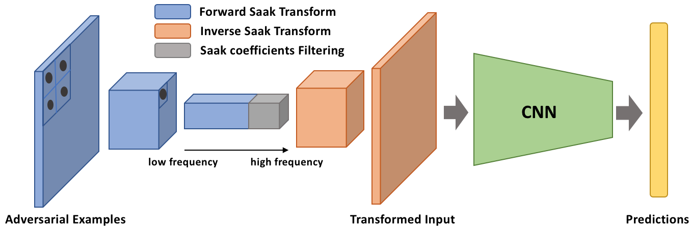
Figure 1: Demonstration of our proposed method to filter out the adversarial perturbations with the multi-stage Saak transform.

II Related Work

Adversarial attacks have been extensively studied since the very earliest attempt [4], which generated L-BFGS adversarial examples by solving a box-constrained optimization problem to fool the neural networks. Goodfellow et al. [16] developed an efficient fast gradient sign method (FGSM) to add adversarial perturbations by computing the gradients of the cost function w.r.t the input. Along this direction, Kurakin et al. [5] proposed a basic iterative method (BIM) that iteratively computes the gradients and takes a small step in the direction (instead of a large one like the FGSM). Later, Dong et al. [17] integrated a momentum term to the BIM to stabilize update directions. Papernot et al. [18] generated an adversarial attack by restricting the $L_{0}$-norm of perturbations. DeepFool (DF) [19] iteratively calculates perturbations to take adversarial images to the decision boundary which is linearized in the high-dimensional space. It was further extended to fool a network with a single universal perturbation [20]. Carlini and Wagner [21] proposed three variants of $CW$ adversarial attacks under $L_{0}$, $L_{2}$ and $L_{\inf}$ distance constraints. Chen et al. [22] generated a strong $L_{1}$ attack by adding elastic-net regularization to combine $L_{1}$ and $L_{2}$ penalty functions. Unlike above-mentioned methods, Xiao et al. [23] proposed a novel method that crafts adversarial examples by applying spatial and locally-smooth transformation instead of focusing on pixel-level change. Su et al. [24] presented a way to attack neural networks by changing only one pixel from each image through a differential evolution algorithm.

Recently, a few defense techniques have been proposed in detecting and defending against adversarial attacks. Papernot et al. [8] proposed a defensive distillation method that uses soft labels from a teacher network to train a student model. Gu and Rigazio [25] applied stacked denoising auto-encoders to reduce adversarial perturbations. Li and Li [26] used cascaded SVM classifiers to classify adversarial examples. They also showed that $3\times 3$ average filters can mitigate adversarial effect. Recently, Tramer et al. [27] achieved good results by training networks with adversarial images generated from different models. Guo et al. [11] applies input transformations such as cropping, bit-depth reduction, JPEG compression and total variance minimization to remove adversarial perturbations. Similarly, Xu et al. [12] proposed several strategies, including median smoothing and bit-depth reduction, to destruct adversarial perturbations spatially. Dziugaite et al. [28] investigated the effect of JPEG compression on adversarial images. Based on that, Akhtar et al. [29] built a perturbation detector using the Discrete Cosine Transform (DCT). Very recently, Liu et al. [13] designed an adversarial-example-oriented table to replace the default quantization table in JPEG compression to remove adversarial noise.

The Saak transform [15] provides an efficient, scalable and robust tool for image representation. It is a representation not derived by differentiation. This makes gradient-based or optimization-based attack difficult to apply. The Saak transform has several advantages over the DCT in removing adversarial perturbations. First, Saak transform kernels are derived from the input data while the ones used in DCT are data independent. Saak kernels trained with clean data from a specific dataset are more effective in removing perturbation noise. Furthermore, the PCA is used in the Saak transform to remove statistical dependency among pixels, which is optimal in theory. The DCT is known to be a low-complexity approximation to the PCA in achieving the desired whitening effect. Finally, the multi-stage Saak transform can preserve the prominent spatial-spectral information of the input data, which contributes to robust classification of attacked images. In this work, we investigate Saak coefficients of each spectral component, and observe that high frequency channels contribute more to adversarial perturbations. We conduct experiments on the CIFAR-10 and the ImageNet datasets and show that our approach outperforms all state-of-the-art approaches.

III Proposed Method

III-A Problem Formulation

Before introducing the proposed method, we formulate the problem of adversarial attacks and defenses with respect to a given neural network. A neural network is denoted by a mapping $\mathbf{y}=f(\mathbf{x})$, where $\mathbf{x}\in\mathbb{R}^{W\times H\times D}$ is and input image of size $W\times H\times D$ and $\mathbf{y}\in\mathbb{N}$ is the predicted output vector. Given neural network model $f$, clean image $\mathbf{x}$ and its ground-truth label $\hat{\mathbf{y}}$, crafting an adversarial example denoted by $\mathbf{x^{\prime}}$ can be described as a box-constraint optimization problem:

$$\min_{\mathbf{x}^{\prime}}{\left\|\mathbf{x}^{\prime}-\mathbf{x}\right\|}_{p},\quad\text{s.t.}\quad\mathbf{y}=\hat{\mathbf{y}},\quad f(\mathbf{x}^{\prime})\neq\hat{\mathbf{y}},$$ (1)

where $\left\|\cdot\right\|$ is the $L_{p}$ norm. Our goal is to find a transformation function $\Psi(\cdot)$ to mitigate the adversarial effect of $\mathbf{x}^{\prime}$. In other words, we aim at obtaining a transformation such that predictions of the transformed adversarial examples are as close to ground-truth labels as possible. Ideally, $f(\Psi(\mathbf{x}^{\prime}))=f(\Psi(\mathbf{x}))=f(\mathbf{x})=\hat{\mathbf{y}}$. In most settings of recent attacks, an adversary can have direct access to the model $f(\mathbf{x})$and attack the model by taking advantage of the gradients of the network w.r.t the input. For this reason, a desired transformation, $\Psi(\cdot)$, should be non-differentiable. This will make attacks on the target model $f(\Psi(\cdot))$ more challenging even if an attacker can access all parameters in $f(\cdot)$ and $\Psi(\cdot)$.

III-B Image Transformation via Saak Coefficients Filtering

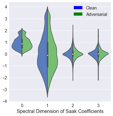
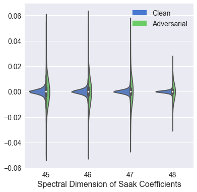
Figure 2: From left to right: The distributions (histograms) of Saak coefficients of clean images and FGSM adversarial examples in four representative low and high spectral components are shown in (a) and (b), respectively. In (a), distributions of Saak coefficients belonging to low spectral dimension 0 to 3 are shown. In (b), distributions of Saak coefficients belonging to high spectral dimension 45 to 48 are shown. The y-axis represents the values of Saak coefficients. As shown in (b), for high spectral components, the Saak coefficients distributions are different between clean and adversarial examples. In (c) and (d), the normalized and the original RMSE (root-mean-squared-error) values between clean and FGSM adversarial examples in different spectral components are shown. The y-axis in both figures represents the spectral dimension of Saak coefficients. In (c), we can observe that clean and adversarial examples have different coefficient values in high spectral dimensions. (These results are obtained from two-stage Saak transform with $2\times 2$ local cuboids.)

Saak Transformation of an image. As shown in the left part of Fig. 1, an image is decomposed into blocks of $2\times 2$ pixels (or local cuboids (LCs) of shape $2\times 2\times k$, where $k$ is the spectral dimension). Then, the KLT transform is conducted on the block (or cuboid) by merging four spatial nodes into one parent node. This process is recursively conducted stage by stage in the forward multi-stage Saak transform. Note that, $2\times 2$ is a typical size of LCs for illustration purpose, we can use arbitrary size in practice. The signed KLT coefficients in each stage are called Saak coefficients. The Saak coefficients are discriminative features of the input image. One can define a multi-stage inverse Saak transform that converts cuboids of lower spatial resolutions and high spectral resolutions to cuboids of higher spatial resolutions and lower spectral resolutions and, eventually, reconstructs the approximate (or original) image depending on whether the lossy (or lossy) Saak transform is adopted.

Saak coefficients as discriminative features. We compare the histogram of Saak coefficient values of clean (in blue) and adversarial images (in green) in four representative low and high spectral components in Figs. 2 (a) and (b), respectively. Following the experiment setup in [13], the adversarial examples are generated using FGSM algorithms on the first 100 correctly classified samples in the CIFAR-10 test set. We remark that similar observations can be found in other adversarial attacks. We see that clean and adversarial images share similar distributions in lower spectral components. However, for high spectral components, adversarial examples have much larger variances than clean examples. These results indicate that high-frequency Saak coefficients have discriminative power in distinguishing adversarial and clean examples. In addition, we show the normalized and the original root-mean-square error of Saak coefficients between clean images and adversarial examples in Figs. 2 (c) and (d), respectively. After normalization by the range of clean Saak coefficients, we see clearly that the difference between clean and adversarially perturbed images primarily lies in high-frequency Saak coefficients. Based on the above observation, we propose to use the multi-stage Saak transform [15] as the transformation function $\Psi(\cdot)$. As mentioned earlier, the Saak transform can offer a joint spatial-spectral representation. It maps a local 3D cuboid into a 1D rectified spectral vector via a one-stage Saak transform. Multiple local 3D cuboids can be transformed in parallel, and the union of them form a global 3D cuboid. The global cuboid consists of two spatial dimensions and one spectral dimension. The one-stage Saak transform consists of two cascaded operations: 1) signal transform via PCA and 2) sign-to-position format conversion. It allows both lossless and lossy transforms. The distance between any two input vectors and that of their corresponding output vectors is preserved at a certain degree. Furthermore, the one-stage Saak transform can be extended to multi-stage Saak transforms by cascading multiple one-stage Saak transforms so as to provide a wide range of spatial-spectral representations and higher order of statistics.

III-C Mathematical Formalization

Mathematically, the Saak-based preprocessing technique can be written as

$$\Psi(\mathbf{x^{\prime}})=S^{-1}(\omega(S(\mathbf{x^{\prime}}))),$$ (2)

where $\mathbf{x}^{\prime}$ is an adversarial example, $S(\cdot)$ and $S^{-1}(\cdot)$ are the forward and inverse multi-stage Saak transforms, respectively, and $\omega(\cdot)$ denote a filtering function to be discussed later. Given Saak coefficients $\theta=S(\mathbf{x^{\prime}})$ in an intermediate stage, one can reconstruct an image using the inverse Saak transform on filtered Saak coefficients denoted by $\omega(S(\mathbf{x^{\prime}}))$. In other words, we convert an adversarial perturbation removal problem into a Saak coefficients filtering problem. We attempt to formalize the idea in Sec. III-B below.

First, we have

$$\begin{split}\left\|\Psi(\textbf{x}^{\prime})-\Psi(\textbf{x})\right\|_{2}&=\left\|S^{-1}(\omega(\theta^{\prime}))-S^{-1}(\omega(\theta))\right\|_{2}\\ &\approx\left\|\omega(\theta^{\prime})-\omega(\theta)\right\|_{2}\\ &=\left\|\omega(\theta_{l}^{\prime})-\omega(\theta_{l})\right\|_{2}+\left\|\omega(\theta_{h}^{\prime})-\omega(\theta_{h})\right\|_{2},\end{split}$$ (3)

where $\theta_{h}$ and $\theta_{l}$ denote the orthogonal subsets of high- and low-frequency Saak coefficients. The approximation is based on the semi-distance preserving property of the inverse Saak transform. Under the assumption that adversarial noise lies in high-frequency regions, which is supported by the discussion in Sec. III-B, we have

$$\begin{split}\left\|\Psi({\textbf{x}}^{\prime})-\Psi({\textbf{x}})\right\|_{2}&=\left\|\theta_{l}^{\prime}-\theta_{l}\right\|_{2}+\left\|\omega(\theta_{h}^{\prime})-\omega(\theta_{h})]\right\|_{2}\\ &\approx\left\|\omega(\theta_{h}^{\prime})-\omega(\theta_{h})\right\|_{2}.\end{split}$$ (4)

Then, if we can design a filter $\omega$ operating on high-frequency components so that the difference of purified Saak coefficients between clean images $\mathbf{x}$ and adversarial images $\mathbf{x^{\prime}}$ is minimized, the difference between clean images and adversarial images can be minimized as well. In other words, the adversarial perturbations are removed. This will be investigated in the next subsection.

III-D Saak Coefficients Filtering

To reduce adversarial perturbations, we propose three high-frequency Saak coefficients filtering strategies to minimize $\omega(\theta_{h}^{\prime})-\omega(\theta_{h})$ in this subsection. They are dynamic-range scaling, truncation, and clipping. Each of them will be detailed below.

As shown in Fig. 2 (b), high-frequency Saak coefficients of clean images tend to have a smaller dynamic range while those of adversarial examples have a larger dynamic range. Thus, the first adversarial perturbation filtering strategy is to re-scale high-frequency Saak coefficients to match the statistics of those of clean images. We expect adversarial perturbations to be mitigated by enforcing the variances of high-frequency Saak coefficients of clean images and adversarial examples to be the same. This is an empirical way to to minimize $\left\|\omega(\theta_{h}^{\prime})-\omega(\theta_{h})\right\|_{2}$.

The second strategy is to truncate high-frequency Saak coefficients. Specifically, we set the least important Saak coefficients to zeros. Since HVS is less sensitive to high-frequency components, image compression algorithms exploit this psycho-visual property by quantizing them with a larger quantization step size. In addition, high-frequency Saak coefficients are very small for clean images, i.e. $\theta_{h}\approx 0$ yet those of adversarial examples may become larger. Based on this observation, we can truncate high-frequency Saak coefficients as a simple way to minimize $\left\|\omega(\theta_{h}^{\prime})-\omega(\theta_{h})\right\|_{2}$.

Setting	(2-2)			(2-4)			(2-5)			(4-2)
Filtered coeff.	40	42	44	640	660	680	2700	2710	2720	580	600	620
clean	84%	84%	68%	96%	96%	91%	96%	95%	95%	96%	95%	91%
FGSM	53%	57%	55%	30%	38%	37%	35%	35%	34%	33%	38%	40%
BIM	65%	69%	62%	49%	61%	61%	63%	63%	65%	54%	58%	64%
DF	77%	77%	65%	83%	83%	82%	86%	86%	86%	84%	83%	81%
$CW_{0}$	63%	61%	45%	56%	64%	66%	65%	62%	62%	58%	65%	64%
$CW_{2}$	84%	81%	66%	94%	92%	89%	93%	91%	90%	89%	93%	85%
$CW_{i}$	82%	80%	67%	90%	90%	85%	92%	92%	92%	87%	89%	85%
All attacks	70.67%	70.83%	60.00%	67.00%	71.33%	70.00%	72.33%	71.50%	71.50%	67.50%	71.00%	69.83%

TABLE I: Comparison of the classification accuracy on the selected CIFAR-10 test set with four Saak transform settings under various attacks, where the filtering strategy is scaling the high-frequency Saak coefficients with a factor $0.25$. The obtained best result is shown in the bold font.

Truncating all high-frequency components might hurt the classification performance on clean data. The third strategy to combat adversarial perturbations is to clip the high-frequency Saak coefficients to a constant small value (instead of zero).

IV Experiments

IV-A Experimental Setup

We conducted experiments on the CIFAR-10 and the ImageNet datasets. The CIFAR-10 dataset [30] consists of colored images drawn from 10 categories with a size of $32\times 32$. The train and test sets contain 50,000 and 10,000 images, respectively. The ImageNet dataset [31] has 1000 classes of various objects. It contains 1.2 million images in the training set, and 50,000 in the validation set. We apply the $224\times 224$ central crop to images from the ImageNet validation set as the input to craft adversarial examples.

To make a fair comparison with recent work [12, 13], we follow the same experiment setup of them and use the DenseNet [32] and the MobileNets [33] as the target models in generating adversarial examples and evaluating all defense methods on CIFAR-10 and ImageNet dataset respectively. We chose six popular and effective attack algorithms: FGSM [16], BIM [5], DF [19], $CW_{0}$, $CW_{2}$ and $CW_{i}$ [21], which generate adversarial examples at different distortion constraints. The least-likely class is chosen to generate targeted CW attacks. Following the setup of [12, 13], we construct a selected set by taking the first 100 correctly classified samples in the test set as seed images to craft adversarial examples, since $CW_{0}$ and $CW_{i}$ attack algorithms are too expensive to run on the whole test set.

We compare our method with recent adversarial defense methods on mitigating adversarial effect that applied input transformations or denoising methods as reported in [12, 13, 11, 34]. Our method is very efficient since it requires no adversarial training, no change on the target model and no back-propagation to train. It can be easily implemented in Python and we will release the code.

IV-B Ablation Studies

As mentioned in [15], the multi-stage Saak transform provides a family of spatial-spectral representations. The intermediate stages in the Saak transform offer different spatial-spectral trade-offs. We first study the effect of different hyper-parameters of the multi-stage Saak transform. We seek to answer two questions: 1) the spatial dimension of 3D local cuboids (LCs) in the Saak transform, and (2) the number of stages used in the Saak transform. We focus on four settings of forward and inverse Saak transforms: 1) spatial dimension $2\times 2$ in 2 stages, 2) spatial dimension $2\times 2$ in 4 stages, 3) spatial dimension $2\times 2$ in 5 stages, and 4) spatial dimension $4\times 4$ in 2 stages. For simplicity, we denote the settings as ({spatial dimension}-{stage}). For example, (2-5) represents the setting of using local cuboid of spatial dimension $2\times 2$ in 5-stage Saak transform. We choose the high-frequency coefficients scaling strategy of a factor $0.25$ in all experiments and report the CIFAR-10 classification results in Table I. For each setting, we consider 3 scenarios in terms of filtered high-frequency Saak coefficeints.

Filtering	Truncation				Clipping by 0.02
Filtered coeff.	2700	2710	2720	2730	2700	2710	2720	2730
clean	92%	92%	92%	91%	95%	94%	92%	91%
FGSM	60%	63%	63%	62%	44%	47%	47%	44%
BIM	72%	69%	73%	71%	67%	66%	69%	67%
DF	86%	87%	88%	86%	86%	85%	84%	84%
$CW_{0}$	71%	70%	68%	69%	69%	68%	68%	68%
$CW_{2}$	91%	90%	90%	90%	91%	91%	91%	91%
$CW_{i}$	89%	90%	90%	90%	91%	91%	92%	91%
All attacks	78.17%	78.17%	78.67%	78.00%	74.67%	74.67%	75.17%	74.17%

TABLE II: Comparison of classification results using the high-frequency Saak coefficient truncation and clipping strategies under various attacks for the selected CIFAR-10 test set (with Saak setting of (2-5)). The obtained best result is shown in the bold font.

Since input images of CIFAR-10 is of spatial dimension $32\times 32$, the spatial dimensions of the output of these settings are $8\times 8$, $2\times 2$, $1\times 1$, and $2\times 2$, respectively. The corresponding spectral dimensions are 53, 853, 3413 and 785. As shown in Table I, we see better defense performance as we increase the filter size or the stage number. The performance are comparable when the output spatial dimensions are the same. We believe that this is related to the receptive field size of the last stage of Saak coefficients used for image reconstruction. The multi-stage Saak transform can incorporate longer-distance pixel correlations to mitigate adversarial perturbations more. For this reason, we choose the 5-stage Saak transform with local cuboids of spatial dimension $2\times 2$ (denoted by (2-5)) in the following experiments as our evaluation baseline.

Defense Methods	FGSM	BIM	DF	$CW_{0}$	$CW_{2}$	$CW_{i}$	All attacks	clean
JPEG [14, 34] (Q=90)	38%	29%	67%	2%	80%	71%	47.83%	94%
Feature Distillation [13]	41%	51%	79%	18%	86%	76%	58.50%	94%
Bit Depth Reduction (5-bit) [12]	17%	13%	40%	0%	47%	19%	22.66%	93%
Bit Depth Reduction (4-bit) [12]	21%	29%	72%	10%	84%	74%	48.33%	93%
Median Smoothing (2x2) [12]	38%	56%	83%	85%	83%	86%	71.83%	89%
Non-local Mean (11-3-4) [12]	27%	46%	76%	11%	88%	84%	55.33%	91%
Cropping [11]	46%	43%	51%	15%	79%	76%	51.66%	86%
TVM [11]	41%	40%	44%	34%	75%	71%	50.83%	92%
Quilting [11]	37%	42%	36%	25%	67%	70%	46.17%	90%
Ours (4-2)	58%	70%	84%	69%	88%	88%	76.17%	90%
Ours (2-5)	63%	73%	88%	68%	90%	90%	78.67%	92%

TABLE III: Comparison of classification results of different defense methods on the selected CIFAR-10 test set.

Defense Methods	FGSM	BIM	DF	$CW_{0}$	$CW_{2}$	$CW_{i}$	All attacks	clean
JPEG [14, 34] (Q=90)	1%	0%	8%	4%	68%	32%	18.83%	70%
Feature Distillation [13]	8%	17%	55%	57%	82%	72%	48.50%	66%
Bit Depth Reduction (5-bit) [12]	2%	0%	21%	18%	66%	60%	27.83%	69%
Bit Depth Reduction (4-bit) [12]	5%	4%	44%	67%	82%	79%	46.83%	68%
Median Smoothing (2x2) [12]	22%	28%	72%	85%	84%	81%	62.00%	65%
Median Smoothing (3x3) [12]	33%	41%	66%	79%	79%	76%	62.33%	62%
Non-local Mean (11-3-4) [12]	10%	25%	57%	47%	86%	82%	51.17%	65%
Ours (4-2)	47%	58%	65%	66%	71%	69%	62.67%	69%
Ours (4-2) + Mean ($2\times 2$)	31%	46%	64%	68%	81%	81%	61.83%	81%
Ours (4-2) + Median ($2\times 2$)	33%	45%	70%	84%	83%	83%	66.33%	86%

TABLE IV: Comparison of classification results of different defense methods on the selected ImageNet test set.

We show the classification accuracy using the other two coefficient filtering strategies; namely, truncation and clipping, under the same baseline setting (2-5) in Table II. By comparing Tables I and II, we see that the coefficient truncation strategy performs the best with a substantial gain over the coefficient scaling and clipping strategies. Thus, we choose truncation strategy as the evaluation method on CIFAR-10 and ImageNet datasets.

IV-C Comparison with State-of-the-Art Methods

We compare our method with other state-of-the-art methods in combating adversarial perturbations for the CIFAR-10 dataset in Table III. We see that our Saak-transform-based method outperforms state-of-the-art methods on all attack types except for the $CW_{0}$ attack by a significant margin. This may be attributed to the fact that the $CW_{0}$ adversarial noise is more prominent as shown in Fig. 3. It is evident that some colored patches in Saak-transform-filtered image are caused by $CW_{0}$ attack which shows that our filtering strategy fails to remove the $CW_{0}$ adversarial noise well since it is already diffused into low-frequency channels. Yet, it is worthwhile to point out our proposed method achieves 90% accuracy on $CW_{2}$ and $CW_{i}$ adversarial examples of CIFAR-10 dataset, which is close to the accuracy on clean data. Moreover, our method is powerful in removing FGSM-based perturbations. Furthermore, we compare different defense methods on the ImageNet dataset in Table IV. Our method outperforms other defense methods when applied alone with the setting of (4-2). In addition, to verify the above conjecture on the $CW_{0}$ attack, we cascade the proposed method with two spatial denoising methods, median and mean smoothing, to further improve the performance. As shown in Table IV, the median smoothing method does boost the performance on the $CW_{0}$ attack significantly. Meanwhile, it improves the classification accuracy on clean data to 86%. These results demonstrate that our solution is complementary to spatial smoothing techniques and, more importantly, can greatly mitigate the adversarial effect without severely hurting the classification performance on clean images unlike other methods. This is highly desirable as a computer vision system is usually unaware whether an input image is maliciously polluted or not.

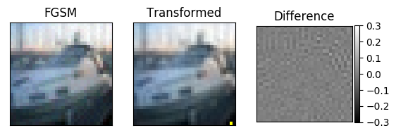
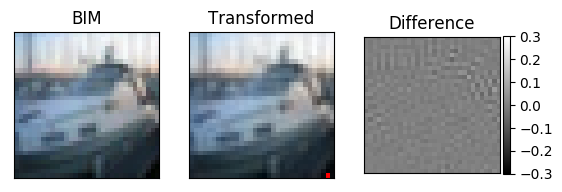
Figure 3: Comparison of adversarial examples and Saak-transform-filtered images on six adversarial attacks with Saak transform setting (4-2) using truncation strategy. Difference image is converted into gray scale.

V Conclusion

We presented a method to filter out adversarial perturbations based on the Saak transform, a state-of-the-art spectral analysis algorithm. It can be used as a light-weight add-on to existing neural networks. The method was comprehensively evaluated in different settings and filtering strategies. It is effective and efficient in defending against adversarial attacks as a result of the following three special characteristics. It is non-differentiable. It does not modify the target model. It requires no adversarial training and no label information. It was shown by experiments that the proposed method outperforms state-of-the-art defense methods by a large margin on both the CIFAR-10 and the ImageNet datasets while maintaining good performance on clean images.

References

- [1] F. Schroff, D. Kalenichenko, and J. Philbin, “Facenet: A unified embedding for face recognition and clustering,” in Proceedings of the IEEE conference on computer vision and pattern recognition, 2015, pp. 815–823.
- [2] H. Xu, Y. Gao, F. Yu, and T. Darrell, “End-to-end learning of driving models from large-scale video datasets,” arXiv preprint, 2016.
- [3] W. Li, R. Zhao, T. Xiao, and X. Wang, “Deepreid: Deep filter pairing neural network for person re-identification,” in Proceedings of the IEEE Conference on Computer Vision and Pattern Recognition, 2014, pp. 152–159.
- [4] C. Szegedy, W. Zaremba, I. Sutskever, J. Bruna, D. Erhan, I. Goodfellow, and R. Fergus, “Intriguing properties of neural networks,” arXiv preprint arXiv:1312.6199, 2013.
- [5] A. Kurakin, I. Goodfellow, and S. Bengio, “Adversarial examples in the physical world,” arXiv preprint arXiv:1607.02533, 2016.
- [6] ——, “Adversarial machine learning at scale,” arXiv preprint arXiv:1611.01236, 2016.
- [7] Y. Liu, X. Chen, C. Liu, and D. Song, “Delving into transferable adversarial examples and black-box attacks,” arXiv preprint arXiv:1611.02770, 2016.
- [8] N. Papernot, P. McDaniel, X. Wu, S. Jha, and A. Swami, “Distillation as a defense to adversarial perturbations against deep neural networks,” in Security and Privacy (SP), 2016 IEEE Symposium on. IEEE, 2016, pp. 582–597.
- [9] A. S. Ross and F. Doshi-Velez, “Improving the adversarial robustness and interpretability of deep neural networks by regularizing their input gradients,” arXiv preprint arXiv:1711.09404, 2017.
- [10] C. Lyu, K. Huang, and H.-N. Liang, “A unified gradient regularization family for adversarial examples,” in Data Mining (ICDM), 2015 IEEE International Conference on. IEEE, 2015, pp. 301–309.
- [11] C. Guo, M. Rana, M. Cissé, and L. van der Maaten, “Countering adversarial images using input transformations,” Proceedings of the International Conference on Learning Representations (ICLR), 2017.
- [12] W. Xu, D. Evans, and Y. Qi, “Feature squeezing: Detecting adversarial examples in deep neural networks,” The Network and Distributed System Security Symposium, 2017.
- [13] Z. Liu, Q. Liu, T. Liu, Y. Wang, and W. Wen, “Feature distillation: Dnn-oriented jpeg compression against adversarial examples,” Proceedings of the 27th International Joint Conference on Artificial Intelligence (IJCAI), 2018.
- [14] N. Das, M. Shanbhogue, S.-T. Chen, F. Hohman, L. Chen, M. E. Kounavis, and D. H. Chau, “Keeping the bad guys out: Protecting and vaccinating deep learning with jpeg compression,” arXiv preprint arXiv:1705.02900, 2017.
- [15] C.-C. J. Kuo and Y. Chen, “On data-driven saak transform,” Journal of Visual Communication and Image Representation, vol. 50, pp. 237–246, 2018.
- [16] I. J. Goodfellow, J. Shlens, and C. Szegedy, “Explaining and harnessing adversarial examples,” Proceedings of the International Conference on Learning Representations (ICLR), 2015.
- [17] Y. Dong, F. Liao, T. Pang, H. Su, X. Hu, J. Li, and J. Zhu, “Boosting adversarial attacks with momentum,” Proceedings of 2018 IEEE Conference on Computer Vision and Pattern Recognition (CVPR), 2018.
- [18] N. Papernot, P. McDaniel, S. Jha, M. Fredrikson, Z. B. Celik, and A. Swami, “The limitations of deep learning in adversarial settings,” in Security and Privacy (EuroS&P), 2016 IEEE European Symposium on. IEEE, 2016, pp. 372–387.
- [19] S. M. Moosavi Dezfooli, A. Fawzi, and P. Frossard, “Deepfool: a simple and accurate method to fool deep neural networks,” in Proceedings of 2016 IEEE Conference on Computer Vision and Pattern Recognition (CVPR), no. EPFL-CONF-218057, 2016.
- [20] S.-M. Moosavi-Dezfooli, A. Fawzi, O. Fawzi, and P. Frossard, “Universal adversarial perturbations,” in Computer Vision and Pattern Recognition (CVPR), 2017 IEEE Conference on. IEEE, 2017, pp. 86–94.
- [21] N. Carlini and D. Wagner, “Towards evaluating the robustness of neural networks,” in Security and Privacy (SP), 2017 IEEE Symposium on. IEEE, 2017, pp. 39–57.
- [22] P.-Y. Chen, Y. Sharma, H. Zhang, J. Yi, and C.-J. Hsieh, “Ead: elastic-net attacks to deep neural networks via adversarial examples,” arXiv preprint arXiv:1709.04114, 2017.
- [23] C. Xiao, J.-Y. Zhu, B. Li, W. He, M. Liu, and D. Song, “Spatially transformed adversarial examples,” Proceedings of the International Conference on Learning Representations (ICLR), 2018.
- [24] J. Su, D. V. Vargas, and S. Kouichi, “One pixel attack for fooling deep neural networks,” arXiv preprint arXiv:1710.08864, 2017.
- [25] S. Gu and L. Rigazio, “Towards deep neural network architectures robust to adversarial examples,” arXiv preprint arXiv:1412.5068, 2014.
- [26] X. Li and F. Li, “Adversarial examples detection in deep networks with convolutional filter statistics,” CoRR, abs/1612.07767, vol. 7, 2016.
- [27] F. Tramèr, A. Kurakin, N. Papernot, D. Boneh, and P. McDaniel, “Ensemble adversarial training: Attacks and defenses,” arXiv preprint arXiv:1705.07204, 2017.
- [28] G. K. Dziugaite, Z. Ghahramani, and D. M. Roy, “A study of the effect of jpg compression on adversarial images,” arXiv preprint arXiv:1608.00853, 2016.
- [29] N. Akhtar, J. Liu, and A. Mian, “Defense against universal adversarial perturbations,” Proceedings of 2018 IEEE Conference on Computer Vision and Pattern Recognition (CVPR), 2018.
- [30] A. Krizhevsky and G. Hinton, “Learning multiple layers of features from tiny images,” 2009.
- [31] J. Deng, W. Dong, R. Socher, L.-J. Li, K. Li, and L. Fei-Fei, “Imagenet: A large-scale hierarchical image database,” in Computer Vision and Pattern Recognition, 2009. CVPR 2009. IEEE Conference on. IEEE, 2009, pp. 248–255.
- [32] G. Huang, Z. Liu, K. Q. Weinberger, and L. van der Maaten, “Densely connected convolutional networks,” in Proceedings of the IEEE conference on computer vision and pattern recognition, vol. 1, no. 2, 2017, p. 3.
- [33] A. G. Howard, M. Zhu, B. Chen, D. Kalenichenko, W. Wang, T. Weyand, M. Andreetto, and H. Adam, “Mobilenets: Efficient convolutional neural networks for mobile vision applications,” arXiv preprint arXiv:1704.04861, 2017.
- [34] G. Karolina Dziugaite, Z. Ghahramani, and D. M. Roy, “A study of the effect of jpg compression on adversarial images,” arXiv preprint arXiv:1608.00853, 2016.