Magnetic field distribution in magnetars

Abstract

Using an axisymmetric numerical code, we perform an extensive study of the magnetic field configurations in non-rotating neutron stars, varying the mass, magnetic field strength and the equation of state. We find that the monopolar (spherically symmetric) part of the norm of the magnetic field can be described by a single profile, that we fit by a simple eighth-order polynomial, as a function of the star’s radius. This new generic profile applies remarkably well to all magnetized neutron star configurations built on hadronic equations of state. We then apply this profile to build magnetized neutron stars in spherical symmetry, using a modified Tolman-Oppenheimer-Volkov (TOV) system of equations. This new formalism produces slightly better results in terms of mass-radius diagrams than previous attempts to add magnetic terms to these equations. However, we show that such approaches are less accurate than usual, non-magnetized TOV models, and that consistent models must depart from spherical symmetry. Thus, our “universal” magnetic field profile is intended to serve as a tool for nuclear physicists to obtain estimates of magnetic field inside neutron stars, as a function of radial depth, in order to deduce its influence on composition and related properties. It possesses the advantage of being based on magnetic field distributions from realistic self-consistent computations, which are solutions of Maxwell’s equations.

I Introduction

The macroscopic structure and observable astrophysical properties of neutron stars depend crucially on its internal composition and thus the properties of dense matter. The Equation of State (EoS) determines global quantities such as observed mass and radius. Transport properties such as thermal conductivity and bulk viscosity have an effect on cooling observations as well as emission of gravitational waves. As we enter an era of multi-messenger astronomy, it is crucial to construct consistent microscopic and macroscopic models in order to correctly interpret astrophysical observations.

There are a large number of astrophysical observations, e.g. soft-gamma repeaters (SGR) or anomalous X-ray pulsars (AXP), that indicate the existence of ultra-magnetized neutron stars or magnetars Kaspi and Beloborodov (2017). While such observations only probe the surface magnetic field, there is no way to measure directly the maximum magnetic field in the interior. Using the simple virial theorem, one may estimate the maximum interior magnetic field to be as high as $10^{18}$ G. If such large fields exist in the interior, they may strongly affect the energy of the charged particles by confining their motion to quantized Landau levels and consequently modify the particle population, transport properties as well as the global structure Avancini et al. (2018); Tolos et al. (2017); Franzon et al. (2016a, b); Gomes et al. (2018, 2017a, 2017b, 2014, 2013); Dexheimer et al. (2012, 2014); Wu et al. (2017); Wei et al. (2017). However, it is necessary to know the magnetic field amplitude at a given location in the star, i.e. a magnetic field distribution, in order to determine its effect on the internal composition and EoS.

The ideal way to tackle that problem would of course be to self-consistently solve the neutron star structure equations endowed with a magnetic field, i.e. combined Einstein, Maxwell and equilibrium equations, together with a magnetic field dependent EoS, as done by Chatterjee et al. Chatterjee et al. (2015). This solution is complicated by the fact that in presence of a magnetic field, the neutron star structure strongly deviates from spherical symmetry and the spherically symmetric Tolman-Oppenheimer-Volkov (TOV) equations are no longer applicable for obtaining the macroscopic structure of a the neutron star Bocquet et al. (1995); Chatterjee et al. (2015); Dexheimer et al. (2017a). For small magnetic fields, perturbative solutions have been developed Konno et al. (1999), but can no longer be applied for field strengths which might influence matter properties.

There have been several attempts to determine neutron star structure assuming an ad hoc profile of the magnetic field, without solving Maxwell’s equations, within the TOV system (see e.g. Casali et al. (2014); Sotani and Tatsumi (2017); Chu et al. (2018)). To that end, many authors employ the parameterization introduced twenty years ago by Bandyopadhyay et al. Bandyopadhyay et al. (1997), where the variation of the magnetic field norm $B$ with baryon number density $n_{B}$ from the centre $B_{c}$ to the surface $B_{s}$ of the star is given by the form

$$B(n_{B}/n_{0})=B_{s}+B_{c}[1-\exp(-\beta(n_{B}/n_{0})^{\gamma})]~{},$$ (1)

with two parameters $\beta$ and $\gamma$, chosen to obtain the desired values of the maximum field at the centre and at the surface. This is an arbitrary profile, which possesses the same symmetries as the baryon density distribution in the star. Parameters $\left(\beta,\gamma\right)$ are chosen such that the surface field is consistent with observations and the maximum field prevailing at the center conforms to the virial theorem.

Lopes and Menezes Lopes and Menezes (2015) later introduced a variable magnetic field, which depends on the energy density rather than on the baryon number density:

$$B=B_{c}\left(\frac{\epsilon_{M}}{\epsilon_{0}}\right)^{\gamma}+B_{s}~{},$$ (2)

where $\epsilon_{M}$ is the energy-density of the matter alone, $\epsilon_{0}$ is the central energy density of the maximum mass non-magnetic neutron star and a parameter $\gamma>0$, arguing that this formalism reduces the number of free parameters from two to one. The authors put forward as additional motivation the fact that it is the energy density and not the number density that is relevant in TOV equations for structure calculations. To account for anisotropy in the shear stress tensor, they applied the above field profile in a formalism Bednarek et al. (2003), where the different elements containing the pressure are “averaged”, leading to shear stress tensor of the form diag($B^{2}/24\pi,B^{2}/24\pi,B^{2}/24\pi$) Dexheimer et al. (2012); Menezes and Lopes (2016). Nevertheless, this approach within the TOV system is still spherically symmetric and the parameter $\gamma$ not related to any experimental or observational constraint. There have also been suggestions of the magnetic field profile being a function of the baryon chemical potential Dexheimer et al. (2012) as:

$$B(\mu_{B})=B_{s}+B_{c}\left[1-\exp(b\frac{(\mu_{B}-938)^{a}}{938})\right]~{},$$ (3)

with $a=2.5$, $b=-4.08\times 10^{-4}$ and $\mu_{B}$ given in MeV. In contrast to the profiles in Eqs. (1,2), such a formula avoids that a phase transition induces a discontinuity in the effective magnetic field.

However, it was subsequently pointed out by Menezes and Alloy Menezes and Alloy (2016) that any of the above ad hoc formulations for magnetic field profiles are physically incorrect since they do not satisfy Maxwell’s equations. In particular, it is obvious that assuming such a magnetic field profile in a spherically symmetric star implies a purely monopolar magnetic vector field distribution, which is incorrect. The inconsistency of this type of approach can be seen, too, by inspecting the most general solution of the equations of hydrostatic equilibrium in general relativity for a spherically symmetric star. In Schwarzschild coordinates, $\left(\bar{t},\bar{r},\bar{\theta},\bar{\varphi}\right)$, the line element reads:

$${\rm d}s^{2}=-e^{-2\Phi}\,{\rm d}\bar{t}^{2}+\left(1-\frac{2Gm}{\bar{r}}\right)^{-1}{\rm d}\bar{r}^{2}+\bar{r}^{2}\left({\rm d}\bar{\theta}^{2}+\sin^{2}\bar{\theta}{\rm d}\bar{\varphi}^{2}\right),$$ (4)

where $m(\bar{r})$ and $\Phi(\bar{r})$ are the two relativistic gravitational potentials defining the metric (at the Newtonian limit, $m$ represents the total mass enclosed in the sphere of radius $\bar{r}$, and $\Phi/c^{2}$ becomes the Newtonian gravitational potential). The resulting coupled system of equations for the star’s structure has been derived by Bowers and Liang Bowers and Liang (1974) and reads

$$\frac{dm}{d\bar{r}} = 4\pi\bar{r}^{2}\varepsilon$$

$$\frac{d\Phi}{d\bar{r}} = \left(1-\frac{2Gm}{\bar{r}c^{2}}\right)^{-1}\left(\frac{Gm}{\bar{r}^{2}}+4\pi G\frac{p_{r}}{c^{2}}\bar{r}\right)$$

$$\frac{dp_{r}}{d\bar{r}} = -\left(\varepsilon+\frac{p_{r}}{c^{2}}\right)\frac{d\Phi}{d\bar{r}}+\frac{2}{\bar{r}}(p_{\perp}-p_{r})~{},$$ (5)

with an energy-momentum tensor of the form $T^{\mu\nu}=\mathrm{diag}(\varepsilon,p_{r},p_{\perp},p_{\perp})$, where $p_{r}$ and $p_{\perp}$ are the radial and tangential pressure components. This is the most general energy-momentum tensor one can use assuming spherical symmetry and it goes beyond the perfect-fluid model, for which $p_{r}=p_{\perp}$. One may be tempted to cast a general electromagnetic energy-momentum tensor assuming a perfect conductor and isotropic matter, and for a magnetic field pointing in $z$-direction (see e.g. Chatterjee et al. (2015)) into this form. However, in the case of the electromagnetic energy-momentum tensor $T^{\theta\theta}\neq T^{\phi\phi}$ (look at Eqs. (23d)-(23e) of Chatterjee et al. (2015)), in clear contradiction with the assumption of Bowers and Liang (5) in spherical symmetry. Another problem arises from the fact that $\lim_{r\to 0}(T^{rr}-T^{\theta\theta})\not=0$ and thus, the last term in Eq. (5) diverges at the origin (from the first line in this equation, one sees that the quantity $m(\bar{r})\sim\bar{r}^{3}$ and therefore $m/\bar{r}^{2}$ does not diverge). This discussion shows that there cannot be any correct description of the magnetic field in spherical symmetry.

Starting from two-dimensional numerical models, Dexheimer et al. Dexheimer et al. (2017b, 2017) performed a fit to the shapes of the magnetic field profiles following the stellar polar direction as a function of the chemical potentials (as in Dexheimer et al. (2012)) by quadratic polynomials instead of exponential ones as

$$B(\mu_{B})=\frac{(a+b\mu_{B}+c\mu_{B}^{2})}{B_{c}^{2}}\mu~{},$$ (6)

where $a,b,c$ are coefficients determined from the numerical fit. Unfortunately, no check of the validity of this fit has been shown in these works for other directions. In Ref. Mallick and Schramm (2014), a density dependent profile is applied within a perturbative axisymmetric approach à la Hartle and Thorne Hartle and Thorne (1968), but without solving Maxwell’s equations. It remains, however, that the star’s deformation due to the magnetic field implies that such a density (or equivalent) dependent profile depends on the direction, thus will be different looking e.g. in the polar or the equatorial direction.

In view of all these intrinsic difficulties, we will not propose here a simple scheme for solving structure equations of magnetized stars – to that end we refer to the publicly available numerical codes assuming axial symmetry Chatterjee et al. (2015); Bucciantini et al. (2014). Instead, since in many cases it might be sufficient to have an idea of the order of the value of the magnetic field strength to test its potential effect on matter properties, our aim is to provide a “universal” magnetic field strength profile from the surface to the interior obtained from the field distribution in a fully self-consistent numerical calculation from one of these codes. Further, we probe the applicability of this profile for determining the structure of magnetized neutron stars in an approximate way in spherical symmetry compared with full numerical structure calculations. As we will show, qualitatively the correct tendency can be reproduced for some NS properties, but to reproduce quantitatively correct results, the full solution has to be applied.

The paper is organized as follows. Sec. II describes our physical models, including the EoSs we use in this manuscript, together with the numerical techniques applied to solve the models. Sec. III provides the magnetic field profiles derived numerically by varying certain physical parameters, to achieve a generic profile for the monopolar part of the norm of the magnetic field. This profile is then applied in Sec. IV to a modified TOV system, to see its effect on NS masses and radii. Finally, Sec. V gives a summary of our work, together with some concluding remarks.

II Formalism and models

In this section, we summarize the numerical approach for self-consistently modelling magnetized neutron stars. More details can be found in in Chatterjee et al. (2015); Bocquet et al. (1995); Chatterjee et al. (2017).

Model	$n_{\rm sat}$	$E_{B}$	$K$	$E_{\rm sym}$	$L$	$M_{\mathit{max}}$	$R_{1.4}$	$\tilde{\Lambda}(q=.8)$
	$(\mathrm{fm}^{-3})$	(MeV)	(MeV)	(MeV)	(MeV)	($M_{\odot}$)	(km)
HS(DD2)	0.149	16.0	243	31.7	55	2.42	13.2	810
SFHoY	0.158	16.2	245	31.6	47	1.99	11.9	399
STOS	0.145	16.3	281	36.9	111	2.23	14.5	1420
BL_EOS	0.17	15.2	190	35.3	76	2.08	12.3	466
SLy9	0.15	15.8	230	32.0	55	2.16	12.5	533
SLy230a	0.16	16.0	230	32.0	44	2.11	11.8	401

Table 1: Saturation density , $n_{\rm sat}$, the binding energy at saturation $E_{B}$, the compression modulus $K$, the symmetry energy, $E_{\rm sym}$ and its slope, $L$, of symmetric nuclear matter are listed for the different EoS models employed. The neutron star maximum gravitational mass and radius at a fiducial mass of $M_{G}=1.4M_{\odot}$ are given for cold spherical stars. $\tilde{\Lambda}$ is the tidal deformability during inspiral of a binary neutron star merger, calculated with the chirp mass as measured for GW170817 Abbott et al. (2017, 2018). $\tilde{\Lambda}$ is only very weakly dependent on the mass ratio of the two stars, $q=M_{1}/M_{2}$ and is given here for a reference value of $q=0.8$ (the same EoS is assumed for both stars). Note that the STOS EoS is as well excluded by the constraints on $\tilde{\Lambda}$ obtained by GW170817 Abbott et al. (2018) as by nuclear physics experiments indicating much lower values for the slope of the symmetry energy Oertel et al. (2017). We will nevertheless keep this EoS model as representative of an extreme case with large neutron star radius and symmetry energy slope.

II.1 Non-rotating magnetized neutron stars in general relativity

Due to the high compactness of neutron stars, we consider models within the theory of general relativity and solve coupled Einstein-Maxwell partial differential equations. We follow the scheme described in Bonazzola et al. (1993), who considered the general case of rotating neutron stars, with the assumptions of stationarity, axial and equatorial symmetry, and circular spacetime, where the metric is given in the quasi-isotropic gauge, different from that used in TOV systems (4), by:

$${\rm d}s^{2} = -N^{2}\,{\rm d}t^{2}+C^{2}r^{2}\sin^{2}\theta\left({\rm d}\varphi-N^{\varphi}\,{\rm d}t\right)^{2}$$ (7)

$$+A^{2}\left({\rm d}r^{2}+r^{2}\,{\rm d}\theta^{2}\right),$$

where $N,N^{\varphi},A$ and $C$ are the relativistic gravitational potentials which are, as all other fields in Secs. II-III, functions of the coordinates $(r,\theta)$ only (independent from the $\varphi$-coordinate).

In this work, we shall restrict ourselves to the case without rotation, which in particular implies that there is no electric field in the models (perfect conductor). Nevertheless, as said in the introduction, the presence of a magnetic field induces a distortion of the stellar structure, which cannot remain spherically symmetric. Due to spacetime symmetries and circularity condition, only two magnetic field geometries can be described within this framework: a purely poloidal magnetic field (see Bocquet et al. (1995)) or a purely toroidal one (see Kiuchi and Yoshida (2008) and later Frieben and Rezzolla (2012)). In this work, we consider only purely poloidal magnetic fields, meaning that the only non-trivial components are $B^{r}(r,\theta)$ and $B^{\theta}(r,\theta)$. This choice results in an asymptotically dipolar magnetic field distribution.

Matter is supposed to be composed of a perfect fluid coupled to the magnetic field. In Chatterjee et al. (2015), it has been shown that the use of a magnetic field dependent EoS and inclusion of magnetization in the equations have negligible effects on neutron star structure, at least up to a polar magnetic field $B_{\rm pole}\sim 5\times 10^{17}$ G (roughly corresponding to to a central magnetic field value $b_{c}\sim 2\times 10^{18}$ G) with a simple quark model EoS. We therefore neglect magnetic field dependency of the EoS and magnetization here, but they could be included in a straightforward way Chatterjee et al. (2015). Matter is also assumed to be perfectly conducting and the magnetic field originates from free currents, moving independently from the perfect fluid. Equilibrium equations are obtained from the divergence-free condition of the energy-momentum tensor, and can be written as a first integral of motion,  Bonazzola et al. (1993); Chatterjee et al. (2015). It is mostly the Lorentz force term in this equilibrium equation which distorts the stellar structure and makes it deviate from spherical symmetry. To summarize, given an equation of state (EoS) for nuclear matter (see Sec. II.3 hereafter), we thus solve the system of coupled Einstein-Maxwell equations, together with magnetostatic equilibrium. These models are then characterized by their gravitational mass ($M_{G}$, see Bonazzola et al. (1993) for a definition), their EoS (see Sec. II.3) and the central magnetic field, $b_{c}$.

II.2 Numerical methods

The equations to be solved to get axisymmetric solutions form a set of six non-linear elliptic (Poisson-like) partial differential equations, coupled together with non-compact support (sources for gravitational field extend up to spatial infinity). These equations are solved using the same procedure as described in Bocquet et al. (1995), employing the numerical library lorene Gourgoulhon et al. (2016) based on spectral methods for the representation of fields and the resolution of partial differential equations (see Grandclément and Novak (2009)).

Numerical accuracy of the axisymmetric solutions is checked through an independent test, the so-called relativistic virial theorem (Bonazzola and Gourgoulhon (1994); Gourgoulhon and Bonazzola (1994)). This gives an upper bound on the relative accuracy of the obtained numerical solution, and we checked that it always remained lower than $10^{-4}$ for the axisymmetric models presented in Sec. III.

II.3 Equations of state

The system of equations described above is closed by the EoS for nuclear matter relating the pressure $p$ to the baryon density $n_{B}$. Our selection of EoSs for the present work has been guided by the idea to represent a large variety of different neutron star compositions and nuclear properties, derived from completely different nuclear physics formalisms. This was done in order to achieve an unbiased universal parameterization applicable to any realistic nuclear EoS. We consider one EoS model resulting from a microscopic calculation (“BL_EOS”) Bombaci and Logoteta (2018). It uses the Brueckner-Hartree-Fock formalism to tackle the many-body-problem and employs chiral interactions for the basic two- and three-body nuclear interactions. In addition, we consider several phenomenological mean field models. These models are unified models in the sense that the crust EoS has been obtained with the same nuclear interaction than the one for the core guaranteeing consistency at the crust-core transition. They include two non-relativistic Skyrme parameterizations (“SLy9”and “SLy230a”)Chabanat (1995); Chabanat et al. (1997) with the crust model from Gulminelli and Raduta (2015), two relativistic mean field models (“STOS” and “HS(DD2)”) Shen et al. (1998); Typel et al. (2010) with the crust obtained from the model in Hempel and Schaffner-Bielich (2010), supposing a temperature of 0.1 keV. The former one contains non-linear interactions whereas the latter one is constructed with density-dependent couplings. One model with hyperons (“SFhoY”) Fortin et al. (2017) completes our list of EoS models. It is a nonlinear model where the crust is again obtained from Ref. Hempel and Schaffner-Bielich (2010). Hyperonic interactions have been chosen to correctly reproduce hypernuclear data and a neutron star maximum mass above current observational limits. Some nuclear and neutron star properties of the different EoS models are listed in Table 1. All EoS data are available from the on-line database CompOSE Typel et al. (2015).

Figure 1: Magnetic field lines in the $(x,z)$-plane for a $M_{G}=2\ M_{\odot}$ neutron star model endowed with a magnetic field which central value is $b_{c}=5\times 10^{17}\ {\rm G}$ and using the SLy203a EoS of Tab. 1. Thick line denotes the surface of the star and the magnetic moment is along the $z$-axis.

III Generic magnetic field profile

The numerical models of neutron stars endowed with a magnetic field described in Sec. II.1 consider two components ($B^{r}$ and $B^{\theta}$) of the magnetic field vector, as measured by the Eulerian observer (see Bocquet et al. (1995) for details). In the case of non-rotating stars considered here, this magnetic field is the same as that measured in the fluid rest-frame, denoted as $b^{r}$ and $b^{\theta}$ in Chatterjee et al. (2015). As an example, the magnetic field distribution of a full neutron star model is displayed in Fig. 1, for a central value of the magnetic field $b_{c}=5\times 10^{17}$ G. The surface of the star (thick line) does not exhibit any significant deviation from spherical shape, but it is clear that the magnetic field distribution is dominated by the dipolar structure and cannot be accurately described by any spherically-symmetric model.

When trying to parameterize the magnetic field profile, the simplest approach is to consider the norm of the magnetic field, namely

$$b=\sqrt{g_{rr}\left(b^{r}\right)^{2}+g_{\theta\theta}\left(b^{\theta}\right)^{2}}=A\sqrt{\left(b^{r}\right)^{2}+\left(b^{\theta}\right)^{2}},$$ (8)

where the relativistic gravitational potential $A(r,\theta)$ has been defined in Eq. (7). Note that $b$ is the quantity that enters the EoSs which take into account magnetization, as explained e.g. in Chatterjee et al. (2015). The central value of this magnetic field norm is denoted as $b_{c}=b(r=0)$ (independent of $\theta$). In the rest of this work, we will consider this field as the main object of our study.

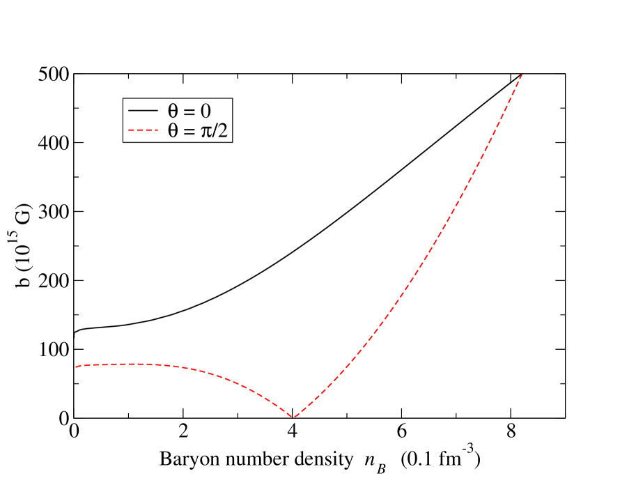
Figure 2: Magnetic field norm $b$ (8) as a function of the baryon density for two angular directions for the same stellar model as in Fig. 1.

As stated in the introduction, several authors have considered a parameterization of the magnetic field norm by the baryon density $n_{B}$. In Fig. 2 we have plotted, for the same neutron star model of $M_{G}=2\ M_{\odot}$ and $b_{c}=5\times 10^{17}$ G as in Fig. 1, the norm of the magnetic field as a function of baryon number density $n_{B}$, along two radial directions: for $\theta=0$ (passing through the pole) and for $\theta=\pi/2$ (passing through the equator). As these two curves show noticeable differences, including close to the center of the star ($n_{B}\sim 0.8\ {\rm fm}^{-3}$), it seems that this type of parameterization can induce some inconsistency when describing magnetic field in a neutron star. We therefore try to improve it and adopt a different approach, taking a multipolar expansion of the magnetic field norm ($Y_{\ell}^{m}(\theta,\varphi)$ being the spherical harmonic functions):

$$b(r,\theta)\simeq\sum_{\ell=0}^{L_{\rm max}}b_{\ell}(r)\times Y_{\ell}^{0}(\theta).$$ (9)

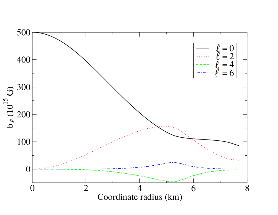
Figure 3: Radial profiles of the first four even multipoles, $b_{\ell},\ell=0,2,4$ and $\ell=6$, see definition (9), of the magnetic field norm $b(r,\theta)$ computed for the stellar model described in Fig. 1. From symmetry arguments odd multipoles are all zero.

In Fig. 3 we have plotted the first four non-zero terms of this multipolar decomposition as functions of the coordinate radius $r$. Note that, because of the symmetry with respect to the equatorial plane, odd-$\ell$ terms in the decomposition (9) are all zero. It appears that, at least in the high-density central regions of the star, the monopolar term $b_{0}(r)$, which is spherically symmetric, is dominant over the others. It is important to stress here that, contrary to the magnetic (vector) field, which has no monopolar part in terms of vector spherical harmonics, the norm of the vector field considered here is a scalar field which can possess a monopolar component.

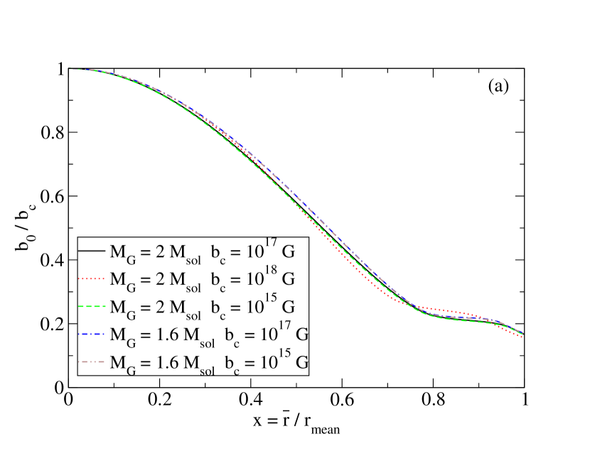
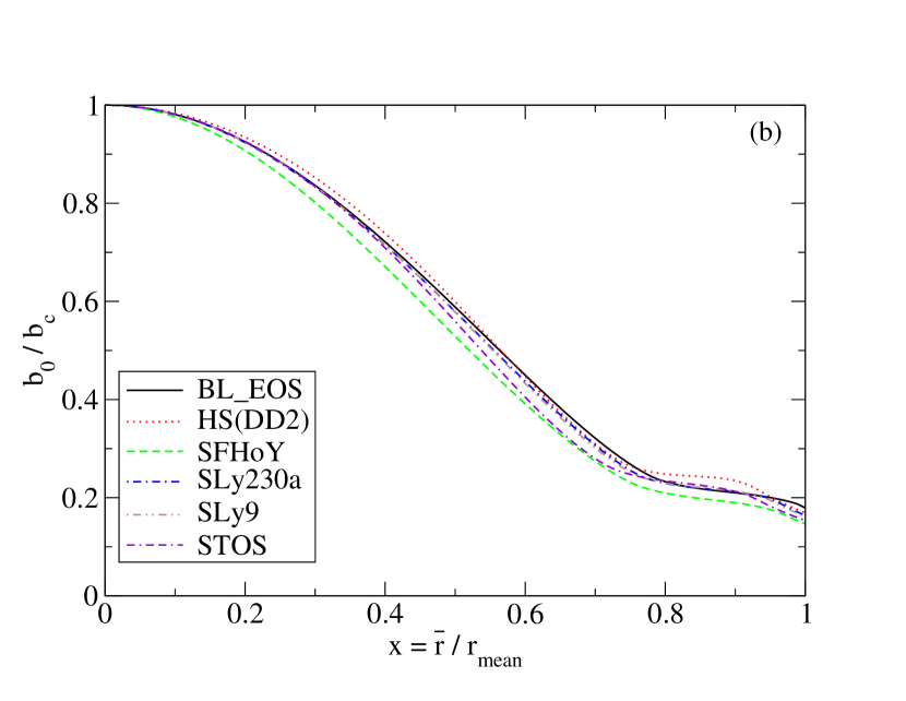
Figure 4: Monopolar part of the magnetic field profile $b_{0}(r)$, normalized to its central value for different magnetized neutron star models, as functions of the radius expressed in Schwarzschild coordinates $\bar{r}$ (see expression (4)) divided by the star’s mean radius (see text). Left panel (a): all models are using SLy230a EoS (see Tab. 1) but have different masses ($1.6\ M_{\odot}$ or $2\ M_{\odot}$) and different central magnetic fields $b_{c}$ ($10^{15}\ \rm{G},10^{17}$ G or $10^{18}$ G). Right panel (b): all are $2\ M_{\odot}$ models, with a central magnetic field $b_{c}=5\times 10^{17}$ G, but with different EoSs, see Tab. 1 for details.

We then look at the behavior of the radial profile of $b_{0}$ when varying the neutron star model in Fig. 4. On the left panel, we vary the gravitational mass of the star (either $1.6\ M_{\odot}$ or $2\ M_{\odot}$), as well as the amplitude of the magnetic field central value $b_{c}$ ($10^{15}$ G, $10^{17}$ G and $10^{18}$ G). On the right panel of Fig. 4, we vary the EoS used in the stellar model, keeping the gravitational mass to be $2\ M_{\odot}$ and the central magnetic field $b_{c}=5\times 10^{17}$ G. These profiles are no longer displayed as functions of the quasi-isotropic coordinate radius $r$, defined by the line element (7), but in view of the application to TOV-systems in Sec. IV, we consider here the Schwarzschild coordinate radius $\bar{r}$, defined by the line element (4). The gauge transformation is obtained numerically and profiles are displayed as functions of this radius divided by the star’s mean radius $r_{\rm mean}$ which is such that the integrated (coordinate-independent) surface of the star reads $\mathcal{A}=4\pi r_{\rm mean}^{2}$. Indeed, when the star gets distorted because of the magnetic field, it is difficult to define uniquely a relevant radius. In that sense, $r_{\rm mean}$ is directly connected to the star’s surface and some of its emission properties.

It is remarkable that, although all possible parameters defining a magnetized stellar model (mass, central magnetic field, EoS) have been varied, all profiles are quite similar and deviate one from another only by a few percent. The only case where a noticeable difference appears is when using quark matter EoS. Therefore, we make the following conjecture: the monopolar part of the norm of the magnetic field follows a universal profile, up to minor variations, when considering different neutron star models with realistic hadronic EoSs. This “universal” profile has been fitted using a simple polynomial:

$$b_{0}(x)=b_{c}\times\left(1-1.6x^{2}-x^{4}+4.2x^{6}-2.4x^{8}\right),$$ (10)

where $x=\bar{r}/r_{\rm mean}$ is the ratio between the radius $\bar{r}$ in Schwarzschild coordinates (4) and the star’s mean (or areal) radius. Let us stress that the aim of the present investigation is to obtain a universal profile for realistic EoSs and that we have therefore excluded polytropic EoSs. A preliminary calculation showed that the general parameterization applicable to the family of realistic EoSs is not applicable directly to the case of polytropes without specific fine tuning.

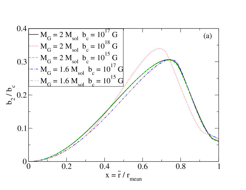
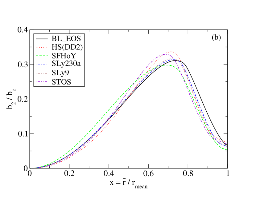
Figure 5: Same as Fig. 4 but for the dipole term $b_{2}(r)$ of the multipolar expansion (9) of the magnetic field norm.

Going further, we display in Fig. 5 profiles for the dipolar part $b_{2}(r)$, defined in Eq. (9). A larger dispersion is visible in these plots, in particular in terms of EoSs (right panel of Fig. 5) and for the largest value of magnetic field ($b_{c}=10^{18}$ G, left panel of Fig. 5). This last point can be understood from the large deformation undergone by the star at this value of central magnetic field, when the contribution from higher-order multipoles starts to become important. Together with Fig. 3, these curves show that spherical symmetry is not a good approximation for strongly magnetized neutron stars, where higher multipoles can have a non-negligible effect. However, the relative robustness of the profiles shown in Fig. 5 indicates that, for not too large magnetic fields, the dipolar correction may be included in an EoS-independent way and some perturbative approach to spherical symmetry may be devised, in a way similar to Konno et al. (1999). We leave these investigations to further studies.

IV Application to a TOV-like system

As discussed in the introduction, it is fundamentally inconsistent to solve spherically symmetric equations for magnetized neutron star models since it completely neglects the star’s deformation due to the electromagnetic field. It is, however, tempting, to have a simple approach at hand which allows at least to qualitatively reproduce the effects of the magnetic field on (some) neutron star properties performing calculations only slightly more complicated than solving TOV equations. To that end, we modify the TOV system by adding the contribution from the magnetic field to the energy density and a Lorentz force term to the equilibrium equation:

$$\frac{dm}{d\bar{r}} = 4\pi\bar{r}^{2}(\varepsilon+\frac{b^{2}}{\mu_{0}})$$

$$\frac{d\Phi}{d\bar{r}} = \left(1-\frac{2Gm}{\bar{r}c^{2}}\right)^{-1}\left(\frac{Gm}{\bar{r}^{2}}+4\pi G\frac{p}{c^{2}}\bar{r}\right)$$

$$\frac{dp}{d\bar{r}} = -\left(\varepsilon+\frac{b^{2}}{\mu_{0}}+\frac{p}{c^{2}}\right)\left(\frac{d\Phi}{d\bar{r}}-L(\bar{r})\right)~{}.$$ (11)

$L(\bar{r})$ denotes here the Lorentz force contribution, which is noted $dM/dr$ in Bonazzola et al. (1993) (see this reference for more details). Note that these equations (11) are not derived from any first principle, but only motivated by Eq.(5), in which we have replaced the diverging term by some phenomenological term, supposed to better take into account the magnetic pressure and the Lorentz force acting on the fluid.

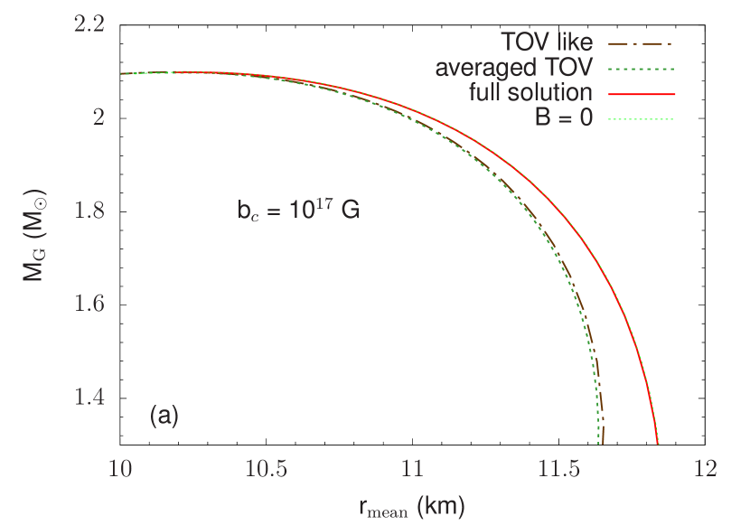
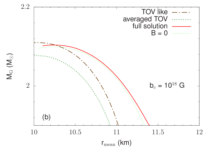
Figure 6: (color online) Gravitational mass vs. mean radius stellar sequences for the TOV-like solution, TOV solution using a directionally-averaged energy momentum tensor (see text) and the exact (axisymmetric) calculation for a central magnetic field of $b_{c}=10^{17}$G (left) and $b_{c}=10^{18}$G (right) employing the SLy230a EoS. Note that, in both figures, the thin-dotted lines ($B=0$) correspond to solutions of the TOV system with no magnetic field at all.

Similar to the magnetic field norm $b$, we found from the full numerical calculations the following parametric form

$$L(\bar{r})=10^{-41}\times b_{c}^{2}\left(-3.8\,x+8.1\,x^{3}-1.6\,x^{5}-2.3\,x^{7}\right)~{},$$ (12)

where $x=\bar{r}/r_{\mathit{mean}}$ and the central magnetic field, $b_{c}$, is given in units of G. For the magnetic field $b$ in Eqs. (11), the profile (10) is applied.

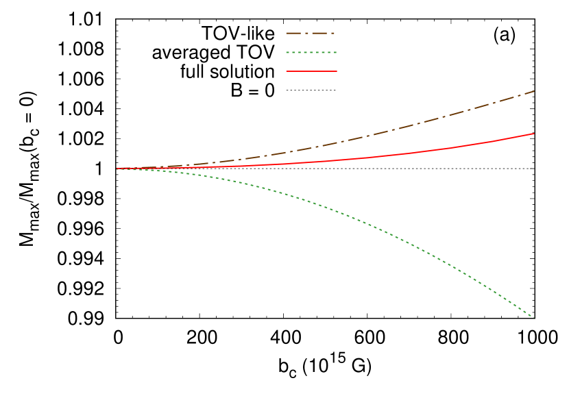
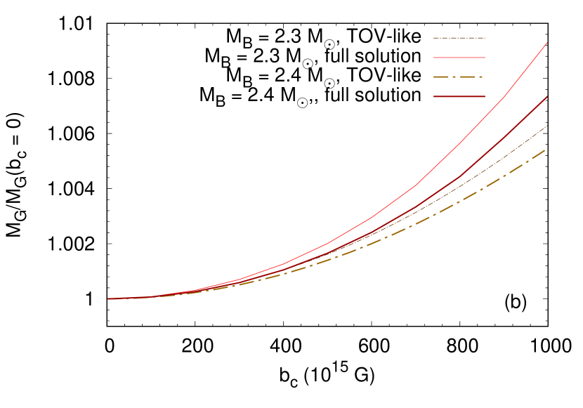
Figure 7: (color online) Left: Comparing the values of the maximum gravitational mass as function of the central magnetic field between our TOV-like approach, the averaged TOV and the full solution. Right: Gravitational mass as function of the central magnetic field for two different values of the baryonic mass.

In order to get an idea of the quality of this “TOV-like” approach, we show in Figs. (6,7) a comparison between stellar sequences (described in mass vs. radius diagrams) obtained with the TOV-like approach in spherical symmetry and the full numerical solution in axial symmetry. In Fig. (6) the gravitational mass vs. the mean radius is displayed for a central magnetic field of $b_{c}=10^{17}$ G (l.h.s.) and $b_{c}=10^{18}$ G (r.h.s). As expected, deviations become larger at smaller masses since the ratio of magnetic to matter pressure increases and thus the stars are more strongly deformed and the relation between the mean radius and the radius of a spherically symmetric configuration is no longer obvious. The same is true if the central magnetic field is increased. For further comparisons, we show in addition the solutions obtained with TOV applying the “averaged” shear stress tensor Bednarek et al. (2003), mentioned in Sec. I, and those obtained without any magnetic field ($B=0$), too. We display here results from the former approach since it has been used several times in the literature Bednarek et al. (2003); Dexheimer et al. (2012); Menezes and Lopes (2016) for studying properties of magnetized stars. Let us emphasize, however, that the procedure to obtain the “averaged” stress-energy tensor is mathematically ill-defined, as it is not possible to directionally “average” elements of a tensor. Moreover, looking at Fig. 6 results with this approach for the mass-radius relation most strongly differ from the full solution. Surprisingly, the usual TOV solution with no magnetic field ($B=0$), on the contrary, very well reproduces the full solution. Thus, although the star becomes strongly deformed, the mean radius is only marginally influenced by the magnetic field.

Masses should be less sensitive to the deformation. As can be seen in Fig. (7), indeed the TOV-like solution for the maximum gravitational mass as well as the gravitational mass for fixed baryon mass as function of the central magnetic field show the correct qualitative behavior. Both increase with $b_{c}$ and the TOV-like approach overestimates the masses up to a factor two in the correction (with respect to the non-magnetized case) at central fields of $b_{c}=10^{18}$G. This difference shows the difficulty of “spherically-symmetric” approaches to model magnetized neutron stars. The limits of the TOV-like approach can be clearly seen in the determination of effects due to the magnetic field. Finally, note that the “averaged” TOV approach gives a wrong qualitative behavior for the dependence of the maximum mass on the central magnetic field value.

Thus, although our investigations can serve as a guideline and reproduce at least for gravitational mass as function of magnetic field the correct qualitative tendency, it should be stressed that it is strongly recommended to use some consistent axisymmetric or three-dimensional approach (e.g. employing publicly available software), to determine properties of magnetized neutron stars or to draw any quantitative conclusion.

V Conclusions

Many attempts can be found in the literature trying to study strongly magnetized neutron stars and to include magnetic field effects on the matter properties. As mentioned in the introduction, most of these investigations suffer from different assumptions and approximations motivated by the complexity of the full system of equations. First, in order to avoid solving Maxwell’s equations in addition to equilibrium and Einstein equations, often an ad hoc profile for the magnetic field is assumed, which has no physical motivation. Second, spherical symmetry is assumed for modelling the star.

In this work, we tackle the first point: we proposed a “universal” parameterization of the magnetic field profile (Eq. 10) as a function of dimensionless stellar radius, obtained from a full numerical calculation of the magnetic field distribution. We tested this profile against several realistic hadronic EoSs, based on completely different approaches, and with different magnetic field strengths in order to confirm its universality. For the case of quark matter EoSs, preliminary investigations showed that although MIT bag models conform to the universality, other quark matter EoSs may not necessarily do so. The profile is intended to serve as a tool for nuclear physicists for practical purposes, namely to obtain an estimate of the maximum field strength as a function of radial depth, within the error bars observed in our study, e.g. in Fig. (4), in order to deduce the composition and related properties.

We applied the proposed magnetic field profile in a modified TOV-like system of equations, that include the contribution of magnetic field to the energy density and pressure, and account for the anisotropy by introducing a Lorentz force term. Compared with full numerical structure calculations, we find that qualitatively the correct tendency is reproduced and quantitatively the agreement is acceptable for large masses and small magnetic fields ($b_{c}\lesssim 10^{17}$ G). However, we find that the standard TOV system with no magnetic field reproduces much better mass-radius relations, even for strong magnetic fields, than any modified TOV system, with poorly defined magnetic corrections. This is mostly due to the fact that the mean radius is only marginally changed by the magnetic field. We thus think that future studies should employ the profile proposed here to conclude about the importance of magnetic field effects on matter properties, and use TOV system at $B=0$ for calculating mass-radius diagrams. For any other property of magnetized stars, we can only recommend the use of a full axisymmetric numerical solution for modelling magnetized neutron stars.