GAMA/G10-COSMOS/3D-HST: Evolution of the galaxy stellar mass function over 12.5Gyrs

Abstract

Using a combined and consistently analysed GAMA, G10-COSMOS, and 3D-HST dataset we explore the evolution of the galaxy stellar-mass function over lookback times $t_{\rm L}\in\left[0.2,12.5\right]{\rm h^{-1}_{70}Gyr}$. We use a series of volume limited samples to fit Schechter functions in bins of $\sim\!$constant lookback time and explore the evolution of the best-fit parameters in both single and two-component cases. In all cases, we employ a fitting procedure that is robust to the effects of Eddington bias and sample variance. Surprisingly, when fitting a two-component Schechter function, we find essentially no evidence of temporal evolution in $M^{\star}$, the two $\alpha$ slope parameters, or the normalisation of the low-mass component. Instead, our fits suggest that the various shape parameters have been exceptionally stable over cosmic time, as has the normalisation of the low-mass component, and that the evolution of the stellar-mass function is well described by a simple build up of the high-mass component over time. When fitting a single component Schechter function, there is an observed evolution in both $M^{\star}$ and $\alpha$, however this is interpreted as being an artefact. Finally, we find that the evolution of the stellar-mass function, and the observed stellar mass density, can be well described by a simple model of constant growth in the high-mass source density over the last $11{\rm h^{-1}_{70}Gyr}$.

1 Introduction

Understanding the redshift evolution of galactic properties is a fundamental method for understanding the growth and evolution of structure over cosmic times. These studies typically explore integrated galaxy parameters such as stellar mass density ($\rho_{\star}$, e.g. Madau & Dickinson, 2014), galaxy population morphological parameters such as the early-type fraction (e.g. Davidzon et al., 2017), individual galaxy evolution parameters such as star formation rates (Driver et al., 2017), environmental parameters such as the galaxy two-point correlation function (e.g. Croom et al., 2005; Zheng et al., 2007) and merger rate (e.g. Bridge et al., 2010), and formation parameters such as the galaxy halo mass function (e.g. Moster et al., 2010). All of these parameters encode complex physics about the formation and growth of galaxies over time.

The integrated galaxy stellar mass density is of particular interest as it can be directly compared to the integrated cosmic star formation history (see Madau & Dickinson, 2014, for an extensive review of such studies). Over the last decade deep near-IR surveys such as the Great Observatories Origins Deep Survey (GOODS; Giavalisco et al., 2004), the MUlti-wavelength Survey by Yale-Chile (MUSYC; Gawiser et al., 2006), the Cosmic Assembly Near-infrared Deep Extragalactic Legacy Survey (CANDELS; Grogin et al., 2011; Koekemoer et al., 2011), the Cosmic Evolution Survey (COSMOS; Scoville et al., 2007) and the FourStar Galaxy Evolution Survey (ZFOURGE; Tomczak et al., 2014), have made studying the properties of high redshift galaxies increasingly accessible to the astronomical community. Meanwhile, large multi-wavelength surveys of the low-redshift universe such as the Galaxy And Mass Assembly (Driver et al., 2011, 2016b), the 2dF Galaxy Redshift Survey (Cole et al., 2001), and Sloan Digital Sky Survey (Bell et al., 2003) have allowed us to explore galaxy properties with high statistical accuracy out to redshifts of $\sim\!0.5$. By combining datasets from these two classes of surveys, we are able to create combined samples that allow us to explore, with high number statistics throughout, the evolution of galactic parameters over a vast redshift range.

In this work, we explore the evolution of the shape of the galaxy stellar mass function (GSMF) using a combination of surveys. In Section 2 we describe the dataset used here. In Section 3 we describe the parameterisation of the GSMF and the fitting methods employed. In Section 4 we present the results of our analysis, with a discussion of the implications of our fits in Section 5, and in Section 6 we provide some concluding remarks.

Throughout this work we use a concordance cosmological model of $\Omega_{\rm M}=0.3$, $\Omega_{\Gamma}=0.7$, ${\rm H_{0}}=70\,{\rm kms^{-1}Mpc^{-1}}$ and ${\rm h_{70}}={\rm H_{0}}/70\,{\rm kms^{-1}Mpc^{-1}}$. All masses are derived/quoted using a time-invariant Chabrier (2003) IMF, Bruzual & Charlot (2003) population synthesis models, and a Charlot & Fall (2000) dust model. All magnitudes are presented in the AB system.

2 Data

In this paper we use the combined GAMA (Driver et al., 2009, 2011, 2017), G10-COSMOS (Davies et al., 2015; Andrews et al., 2017), and 3D-HST (Brammer et al., 2012; Momcheva et al., 2016; Skelton et al., 2014) dataset described in Driver et al. (2017). The dataset combines these three highly complementary surveys which comprehensively sample the low-, mid-, and high-redshift universe respectively. Importantly, each dataset has been analysed in a consistent way, making this dataset somewhat distinct from other large compilations of data presented and analysed in the literature (e.g. Rodríguez-Puebla et al., 2017). The dataset primarily comprises of spectral energy distributions (SEDs) for all galaxies in each of these surveys, and with this dataset Driver et al. (2017) were able to compile a statistically representative sample of galaxies for 19 consecutive bins of redshift spanning the range $z\in\left[0.02,5.00\right]$, which equates to lookback times of $t_{\rm trav}\in\left[0.28,12.31\right]\,{\rm h_{70}^{-1}\,Gyr}$.

A full description of the dataset, including a discussion of systematic effects such as redshift and magnitude completeness, is available in Driver et al. (2017). Nonetheless here we provide a brief overview of the dataset, including summarising the methods of our photometric and SED analyses, before describing the methods of analysis used in this work.

The GAMA and G10-COSMOS data described in Driver et al. (2017) both utilise photometry measured using the lambdar software (Wright et al., 2016) in 21 and 22 filters respectively. lambdar is a bespoke photometric program which was developed specifically to address the challenge of measuring consistent matched aperture photometry on images that are neither seeing nor pixel matched, while performing robust deblending, sky removal, and uncertainty estimation. This is achieved within lambdar by deblending seeing convolved input apertures, generated independently for each input-image pixel grid, with neighbouring galaxies and/or contaminants in an iterative manner. Uncertainties are calculated incorporating shot noise, robust sky estimation using per-galaxy local annuli, and estimation of correlated noise using per-galaxy local blanks. Full description of the processes employed by lambdar can be found in Wright et al. (2016), and the program’s application to GAMA and G10-COSMOS can be found in Wright et al. (2016) and Andrews et al. (2017) respectively. Photometry in the 3D-HST fields are downloaded from the 3D-HST website (http://3dhst.research.yale.edu), rather than being calculated directly from the imaging using lambdar. This represents the only part of our analysis from photometry to final mass function estimation that involves possibly inconsistent measurement methods. Our three datasets are generated from each survey using simple optical flux-limits, prior to the application of mass limits to generate volume-complete samples. For GAMA, G10-COSMOS and 3D-HST these optical selection limits are: $r<19.8$mag, $i\leq 25$mag and F$814$W$\leq 26.0$mag.

Prior to mass estimation we perform an additional cleaning of AGN contaminated sources within the G10-COSMOS and 3D-HST datasets using the formalism described by Donley et al. (2012), as these sources can lead to biases in our mass estimates. We also reject radio loud sources using the prescription of Seymour et al. (2008) in the G10-COSMOS sample. Finally, completeness of the variable-depth 3D-HST dataset is verified by comparison to deep HST number counts from the literature, and is found to be highly complete (within expected cosmic variance) to our adopted magnitude limit of F$160$W$=26.0$mag. Each of these selections is described in detail in Driver et al. (2017).

Each of these photometric datasets is then fit using the SED modeling program magphys (da Cunha et al., 2008) using spectroscopic redshifts (for: all GAMA, some G10-COSMOS, some 3D-HST), GRISM redshifts (for some 3D-HST), and/or photometric redshifts (for: most G10-COSMOS, most 3D-HST). magphys performs an energy balance of observed stellar-origin light with that emitted from warm- and cold-dust, in order to recover the unobscured galaxy stellar mass from observed fluxes. For our fits, we implement the standard magphys template library for each dataset, and then perform an additional run of our 3D-HST dataset using the high-redshift magphys template set. The best fitting template, as determined by the template with the minimum $\chi_{\rm r}^{2}$, for each 3D-HST source is then selected. In practice, 97 percent of the 3D-HST sources are optimally fit by a standard magphys template.

magphys outputs per-galaxy posterior probability distributions for each model parameter, which we then use for parameter inference. Specifically, we use the median of the magphys posterior samples for all parameter inferences, and use the $16^{\rm th}$ to $84^{\rm th}$ percentile range of the posterior samples to define each parameter’s uncertainty. Full description of the application of magphys to this combined dataset is given in Driver et al. (2017).

SED measurements of the galaxies in each dataset provide us with per-galaxy estimates of the stellar mass, star formation history, and dust mass, although in this work we focus solely on the estimated stellar masses. Given the different survey areas and depths, we can utilise these data to generate the stellar mass function over a range of redshifts: the wide area of the GAMA survey provides good sampling of, in particular, the high mass end of the mass function at low redshift, and the deep but narrow G10-COSMOS and 3D-HST surveys provide significant information of the low mass end of the GSMF at low redshift. These deep studies then transition to providing information about the higher mass end of the mass function at high redshift. In this work, as in Driver et al. (2017), we use only volume-complete samples of the full dataset at each redshift interval, thus significantly reducing the possible number of systematic biases that may affect our analysis. Mass completeness limits in each of the datasets have been calculated assuming that the galaxy stellar mass functions exhibit no considerable down-turn over the masses probed in this work. Using this assumption-driven approach, per-dataset per-bin completeness limits used in this work were estimated by Driver et al. (2017) by truncating each dataset to masses exclusively above where a downturn in the mass function is observed.This assumption-driven approach is less rigorous than other methods of mass completeness estimation in the literature (see, e.g., Marchesini et al., 2009; Muzzin et al., 2013; Ilbert et al., 2013; Tomczak et al., 2014; Skelton et al., 2014), however is unlikely to bias our analysis over the mass ranges we explore. This method of estimating mass completeness limits is likely to cause us to over-estimate the mass down to which our samples are complete, as, if a down-turn does exist, this will be interpreted as incompleteness and our analysis truncated prior to this downturn. Additionally, this method is vindicated in the first 13 bins of our analysis by the overlap between the various datasets, and is further bolstered at low-redshift where our GAMA mass limits are in reasonable agreement with more rigorously determined limits for the same sample (Baldry et al., 2018; Wright et al., 2017). Nonetheless, the assumption is most susceptible to error in the highest redshift and lowest mass sections of our analysis; precisely the parts where we have no additional corroborating data. As such, we must recognise the possibility that the analysis in these areas is susceptible to error.

Figure 1 shows our combined dataset for each of the redshift bins, with shot and sample-variance uncertainties indicated as the per-bin error bars. Each panel shows the observed number density for each of the surveys, binned in stellar mass, along with the individual monte-carlo+bootstrap fits coloured by reduced $\chi^{2}$ (more details on this are given in Section 3). These panels highlight the value of this combined dataset: even in regions where one or two of our datasets are lacking in completeness (due to, for example, poor sampling due to a limited survey area; see the 3D-HST data in redshift bin 4), we have sufficient complementarity between the three surveys that there is no difficulty in estimating the completely free two-component Schechter (1976) function.

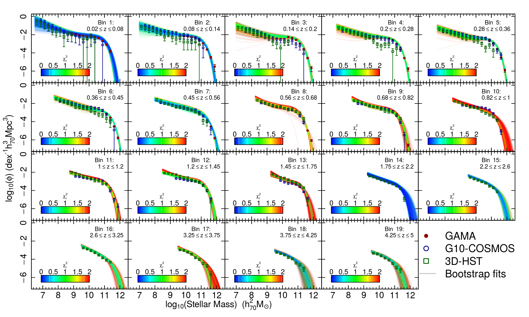
Figure 1: The two-component Schechter function fits to our combined GAMA (red), G10-COSMOS (blue), and 3D-HST (green) dataset. Each panel shows a redshift bin (limits are annotated) with the fitted data, per survey, and the results from the bootstrapped fitting procedure (lines; coloured by fit reduced $\chi^{2}$). Uncertainties on the datasets are determined by the cosmic variance uncertainty of each survey within the relevant redshift interval, and the shot noise per mass bin. Redshift bins 3 and 4 show considerable drops in number density at high masses in G10-COSMOS and 3D-HST. However, even in these cases, the optimisation is able to borrow strength from the complementary GAMA dataset and converge on appropriate fits.

3 Fitting the galaxy stellar mass function

Fitting the Schechter (1976) function to our combined dataset requires careful consideration of each individual dataset’s sample variance uncertainty and selection bias. To account for these, we invoke a fitting method that allows each sample to be fit with its own mass limit and independent perturbation of the normalisation (according to the expected sample variance).

We also wish to incorporate our ignorance of precise stellar masses, and the expected Eddington bias of our samples, into the fitting procedure as well. To do this we invoke a combined monte-carlo+bootstrap simulation method, applied in bins of redshift, using the following steps at each realisation. Starting from the raw data, we select those data within the redshift bin, and perturb every source’s stellar mass according to our magphys fit uncertainty. We then make a bootstrap realisation of this perturbed sample, which results in our fit data for this realisation. Next we bin the three surveys by stellar mass individually, discarding bins below each survey’s mass limit, and divide the number counts by the volume probed, per survey, over this redshift interval. We then perturb each set of binned data by the expected sample variance uncertainty as reported by Driver et al. (2017). These binned data points are then fit with a Schechter function using the quasi-Newton optimisation algorithm of Byrd et al. (1995), which allows box-constraint of optimisation parameters. We select these box constraints using previous results from the literature. For all fits we provide box constraints of $M^{\star}\in\left[10,11.5\right]$ and $\phi^{\star}\in\left[0,1\right]$. For our single-component fits we also constrain $\alpha\in\left[-2,1.5\right]$, and in the two-component case the individual $\alpha$’s are required to be $\alpha_{1}\in\left[-1.1,1.5\right]$ and $\alpha_{2}\in\left[-2,-0.9\right]$, thereby ensuring that the two components do not flip places during optimisation, and discouraging fits with degenerate components. The resulting fit parameters are stored, with uncertainties derived from the optimisation hessian matrix, and the next realisation is begun. We perform $1001$ of these combined monte-carlo+bootstrap realisations per redshift bin. For our final fit parameters and uncertainties we take the 1/$\chi^{2}$-weighted median of all converged fit parameters, and use the similarly weighted $16^{\rm th}$ to $84^{\rm th}$ percentile range for our parameter uncertainties. By using an optimisation procedure such as this, we are able to simultaneously fit all of our three surveys’ data. This allows for better optimisation than would be possible by fitting each sample independently, as the three highly complementary surveys provide constraints of different parts of the Schechter function.

We explore the observed evolution of Schechter function parameters for both a single and two-component Schechter function, and in both cases have all parameters free (within the box-limits specified above). In each of our optimisations, we maximise the likelihood of the data with respect to a convolved version of the Schechter function (with $\sigma_{\rm conv}=0.1$dex) to account for Eddington bias in our samples (Driver et al., 2017).

The two-component Schechter function is visually a much better description of the data at low-redshift, as can be seen by the clear plateau in the mass functions, and has been adopted almost unanimously as the appropriate descriptor of the GSMF there (see, e.g., Baldry et al., 2008, 2012; Davidzon et al., 2017; Wright et al., 2017). Conversely, at high-redshift the GSMF is frequently argued to be well described by a single component Schechter function, which is often used for fitting mass functions there (see, e.g., Song et al., 2016; Grazian et al., 2015; Davidzon et al., 2017). In our analysis, rather than assume a particular Schechter function formalism for different redshift bins, we opt to fit both single and two-component functions to each of our redshift bins, and provide fit parameters and goodness of fit statistics for each. By presenting both datasets in this way, we aim to explore how the mass function evolves under both assumptions without possibly uncertain restrictions.

At low redshift, the combination of highly-complete GAMA data and the deep G10-COSMOS and 3D-HST data allows us to simultaneously constrain the exponential cutoff of the GSMF (principally parameterised by the $M^{\star}$ parameter), and the slope parameter(s) $\alpha_{i}$. However at high redshift our constraint on the slope parameter is less robust, as the data only extend to $\sim\!1$dex below $M^{\star}$. In these higher-redshift bins, one might expect that the two-component fits would become extremely noisy, as the optimisation has far too much freedom given the data; another reason to perform optimisations using both functional forms. We note, however, that our choice of limiting values on the normalisation parameter allows the optimiser to explore single component solutions even in the two-component optimisation. All individual fit parameters and reduced $\chi^{2}$ values are presented in Appendix A.

In addition to fitting our two different Schechter forms, we also make some further assumptions that allow us to better constrain the Schechter function form at each redshift interval. If we assume that redshift evolution of each parameter should a-priori be a smooth function, then we can fit the redshift evolution of each parameter with a simple function and use this to generate a less-noisy estimate of how the Schechter function evolves over cosmic time. Therefore, after establishing our best-fit Schechter parameters in each redshift bin, we also fit a quadratic function to the redshift evolution of each parameter, and show the Schechter function evolution using these best-fit functions. This regression fit to the individual parameters is not largely different to other (iterative) regression procedures invoked in the literature (see, e.g., Drory & Alvarez, 2008; Leja et al., 2015). We shown our regressed fits (and uncertainties) alongside our individual optimisations, and the fit parameters are also presented in Appendix A.

4 Results

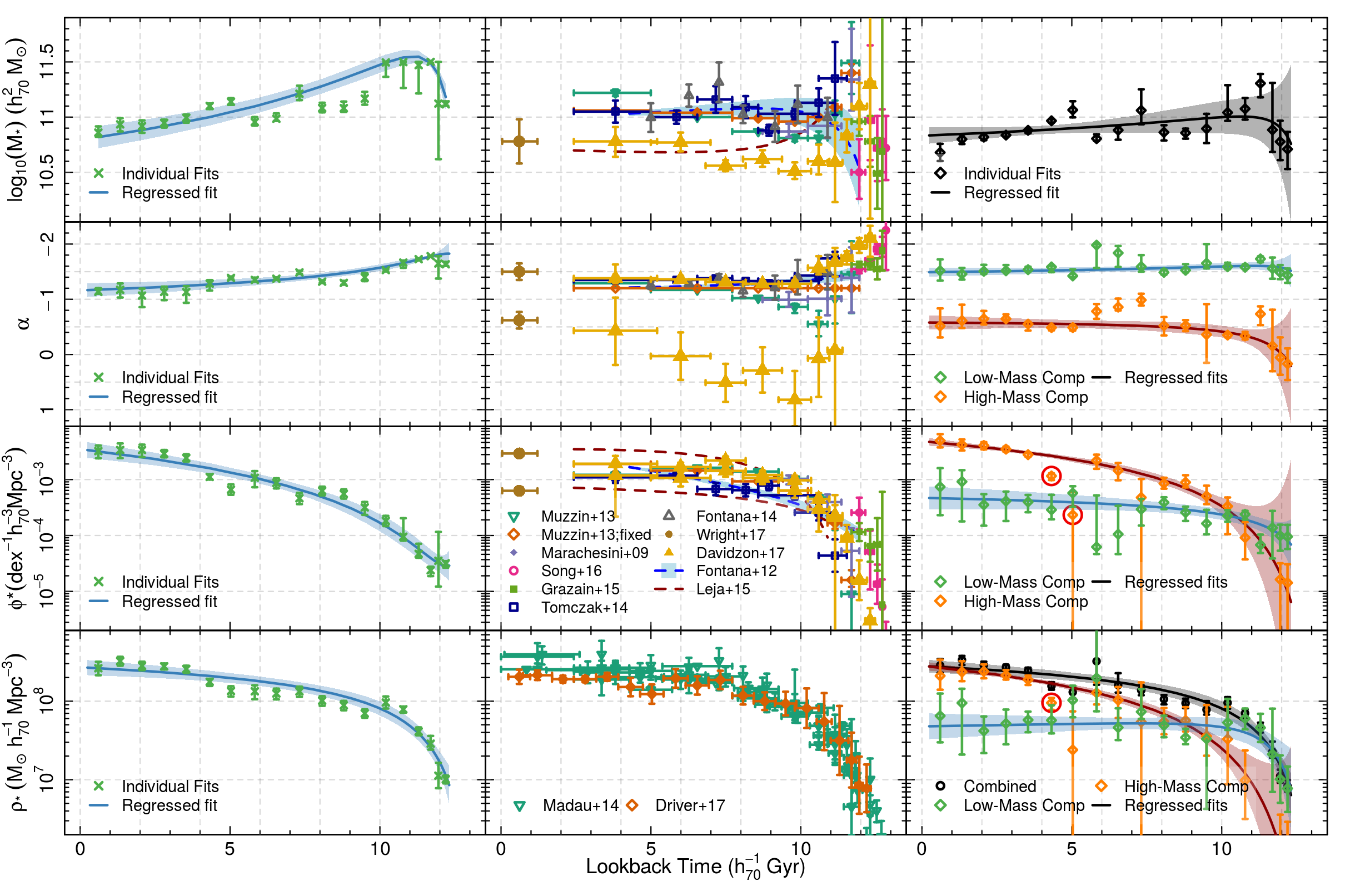
Figure 2: Evolution of the Schechter function parameters, and of the integrated stellar mass density, as a function of lookback time. Center column: Literature compendium of the evolution of each parameter over time. Relevant sources to the Schechter parameter evolution panels are annotated in the $\phi^{\star}$ panel. In $\rho_{\star}$, we show only the compendium of Madau & Dickinson (2014) and the previous results using this dataset from Driver et al. (2017). Left column: Results from our single component Schechter function fits to the dataset. Individual optimisations per bin are shown as points, with uncertainties showing the $\pm 1\sigma$ confidence region determined from the individual bootstrap fits weighted by their $\chi_{\rm r}^{2}$. Our regressions are shown as lines with a shaded uncertainty region. Right column: Results from our two-component Schechter function fits to the dataset. Points and lines here are the same as in the center column, except now there are multiple components being shown in the $\phi^{\star}$ and $\alpha$ panels. Points circled in red are clipped prior to the estimation of the regression fit, as they are in high-tension with the other data. All data points here are provided as supplementary data with this paper. Regression fits are given in Appendix A.

Figure 2 shows the evolution of our Schechter function parameters $M^{\star}$, $\phi^{\star}$, and $\alpha_{i}$, as well as the evolution of the integrated stellar mass density ( which is derived using the analytical integration of the Schechter function fits over all masses). In the figure, we show a compilation of literature values for each parameter (center), as well as our single (left) and two-component (right) fits, separated to aid clarity. The individual data are shown with uncertainties, as described in Section 3. The regression fits are shown with the uncertainty regions also shown as shaded regions around the best fit line. We can see that, in all cases, the fits are best constrained in the low-to-mid redshift bins, and that the fit uncertainties increase significantly beyond lookback times of $\sim\!11\,h_{70}^{-1}\,{\rm Gyr}$.

Looking first at our two-component fits, we see a surprising lack of evolution in all the shape parameters within our fits. Our regressed fit in $M^{\star}$ is consistent with being flat, although a pragmatic interpretation would likely be that there has been a very slight decrease in the value of $M^{\star}$ over the last $\sim\!11.5\,h_{70}^{-1}\,{\rm Gyr}$. Our fit also exhibits a downturn at higher redshifts, however the constraint here is sufficiently weak that interpreting this as a real feature is difficult.

The single component fit shows a somewhat higher $M^{\star}$ than the two-component fit at essentially all times, indicating a bias that can be induced when fitting single component Schechter functions (even high redshift) to data that should likely be fit with more components. The fits also move to significantly higher values of $M^{\star}$ at early times, causing the regression to behave somewhat poorly. We note that this trend is also evident in the literature; studies that have invoked a two-component Schechter function ( e.g.  Leja et al., 2015; Wright et al., 2017; Davidzon et al., 2017) show systematically lower values of $M^{\star}$ than those that fit only a single component ( e.g.  Fontana et al., 2006; Tomczak et al., 2014). This trend is exacerbated by the degeneracy between $M^{\star}$ and $\alpha$, which gets stronger as $\alpha$ approaches a value of -2 (as it does in the high-redshift single component fits). For these reasons alone, we believe that there is a clear motivation to describe the shape of the Schechter function with two components (at least; see Moffett et al., 2016; Kelvin et al., 2014), even out to high redshifts.

The two-component slope parameters $\alpha_{i}$ also shows little evidence of evolution. The low-mass component in particular is impressively stable over cosmic time, showing only a minor flattening over the last $11\,h_{70}^{-1}\,{\rm Gyr}$. Conversely, our single component fits (and the single component regressed model) show an appreciable evolution, and one that shows appreciable steepening of the mass function slope (particularly at high-redshift). We argue that this observed evolution is an artefact. At low-redshift the mass function is poorly described by a single component fit, and the slope parameter is flattened by the plateau of the mass function. Interestingly, at high-redshift, our single-component fits prefer the same increase in slope and $M^{\star}$ as is often seen in the literature, while our two-component fits show no such effect. This result is seen particularly well in the recent work of Davidzon et al. (2017), who see their Schechter function slope and $M^{\star}$ grow significantly steeper and more massive, respectively, in their highest 3 redshift bins where they transition from a two- to single-component fit. Meanwhile our observed fits are in agreement with other studies that push to the estimation of the GSMF to high redshift (Song et al., 2016; Grazian et al., 2015). Finally, our high-mass component shows a slight evolution to a steeper slope over the last $11\,h_{70}^{-1}\,{\rm Gyr}$, however is also reasonably consistent with no evolution.

The value of $\phi^{\star}$ shows the strongest evolution of any of our fitted parameters. In the case of our two-component fits, we observe a marginal decrease in the observed number density of the low-mass component over the last $12\,h_{70}^{-1}\,{\rm Gyr}$, followed by a downturn in the evolution at the highest redshifts. In contrast to this observed stability, the high mass component evolves significantly and with more rapidity. The result of this is that the high mass component begins with little contribution to the mass density, and then builds up to become the dominant component (in mass) at $\sim\!8.5\,h_{70}^{-1}\,{\rm Gyr}$ lookback time. This evolution is seen strongly both in our regressed fits and the individual parameter estimates, with the exception of two outlier bins at $\sim\!4.5$ and $5.0\,h_{70}^{-1}\,{\rm Gyr}$, which are circled red in Figure 2. These bins are both clipped prior to fitting the regression fit to the high-mass component evolution of $\phi^{\star}$, and the former bin is also clipped prior to fitting the regression fit to the high-mass component evolution of the stellar mass density. We note also that this evolution is particularly well matched to the model presented in Leja et al. (2015), although our estimates of other parameters differ somewhat and therefore our resulting mass density evolution is somewhat different to that which is presented there.

Further, comparing the goodness-of-fit of both our single and two-component fits, we see that all bins have reduced-$\chi^{2}$ values that overlap. While one may be inclined to argue that this indicates that our fits are agnostic to the choice of single- or two-component fits in all bins (and, indeed, this is likely true in most of our higher-redshift bins), it is important to note the considerable covariance between the two sets of $\chi_{\rm r}^{2}$ values. In most bins where we have at least two complementary datasets, the dominating source of scatter in our presented $\chi_{\rm r}^{2}$ values is the tension between each of the individual datasets, induced by our cosmic variance perturbation. This can be seen in Figure 1 and in Tables 1 and 2, whereby we see jointly higher absolute values and scatter of $\chi_{\rm r}^{2}$ in bins which are initially in tension; compare, for example, the scatter on our $\chi_{\rm r}^{2}$ values in bins $2$ and $3$, or $6$ and $7$, for both sets of fits. This coherent scatter induces covariance between the $\chi_{\rm r}^{2}$ values in each model, making simple inference regarding model superiority difficult. As such, rather than propose a particular model as being better fitting than another, we instead focus on what we can learn from the evolution of the two models independently.

Finally, we calculate the value of the stellar mass density parameter $\rho_{\star}$ for each of our fits, again using the analytic integral of the fits over all masses. The density parameter proves extremely robust to our different models and fits; all of our fits show a similar evolution and reasonable agreement with previous work from the literature. This is not surprising as the main contribution to mass density at each epoch tends to be from $M\eqsim M^{\star}$ galaxies (and this region is typically well modelled in all the fits). Nonetheless, the stochasticity is removed in our regressed models, and we can see that these values follow the literature well. Interestingly we note that our fits find a surplus of mass density at low redshift with respect to that reported in Driver et al. (2017), and in doing so our fits remove any disparity seen between their low redshift bins and the literature.

All fit results and regression functions are provided in Appendix A.

5 Discussion

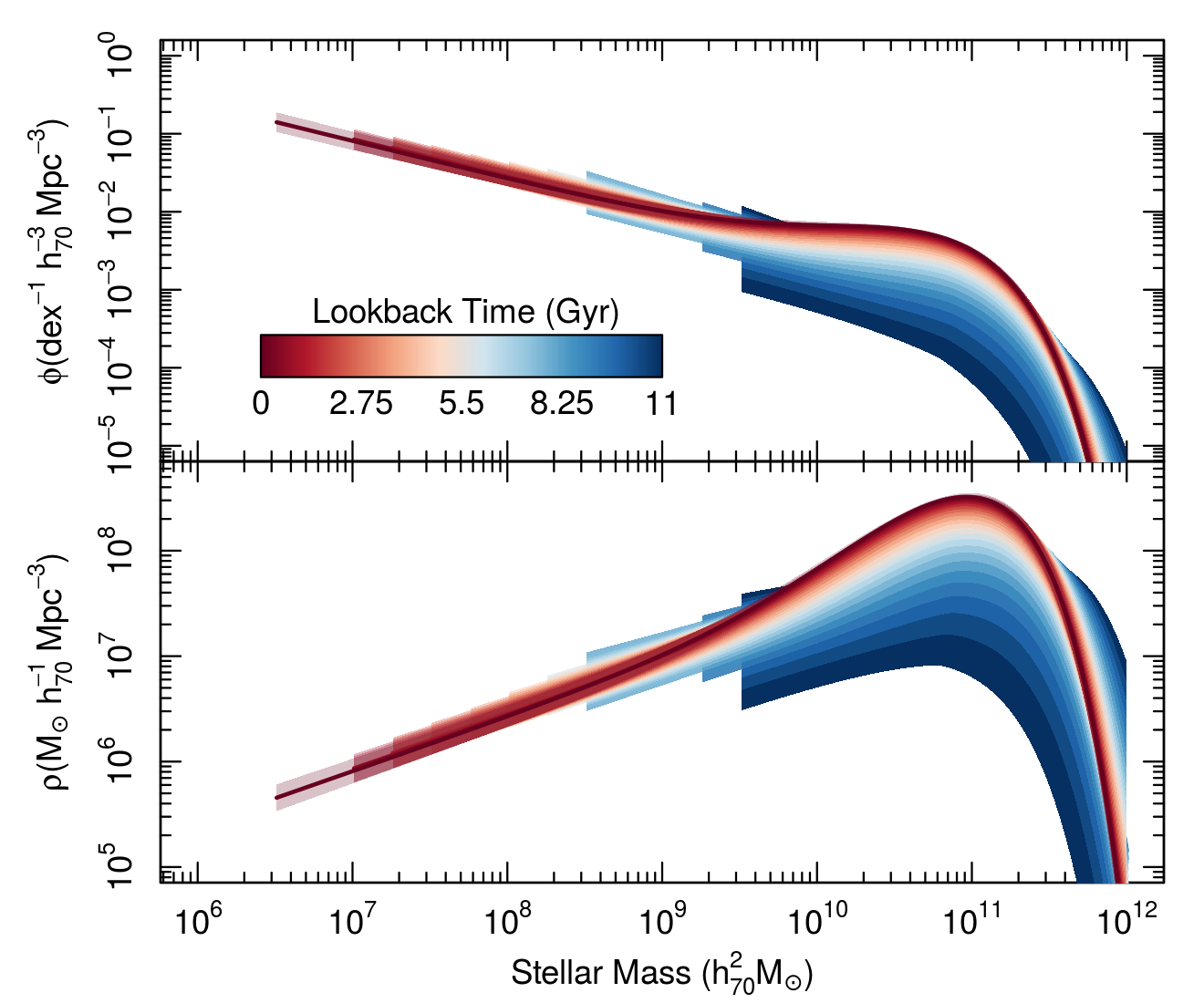
Figure 3: Evolution of the Schechter function over $\sim\!11\,h_{70}^{-1}\,{\rm Gyr}$ (an animated version is provided as supplementary data) Moving forward through time, as determined using the regressed Schechter parameters from Figure 2. At each redshift bin we show the model over only the region where we have data. The upper panel shows the evolution of galaxy number density $\phi$, while the lower panel shows the evolution of the galaxy mass density $\rho$. Uncertainty regions (shaded) show the full allowed region of the fit parameters assuming no covariance, and so are particularly conservative. The figure demonstrates clearly the stability of the Schechter function faint-end slope over time, with only a modest flatting of the number density slope at late times. The evolution is well described by a simple build up of mass in the high-mass component over cosmic time. Similarly, the evolution of mass density is seen to be almost entirely driven by the build-up of the high-mass component, around $M^{\star}$.

In Figure 3 we show graphically the evolution of our fitted Schechter functions, in both number and mass density, over the last 11 Gyr (i.e. in the regime where the evolutional regression fits from Figure 2 are well constrained). In the figure, we can see the striking stability of the mass function over this lookback baseline, with only the high-mass component showing a gradual growth over time. To show this clearer, we provide an animation of this mass function evolution figure in the supplementary material.

The stability of the two-component shape parameters, and the observed evolution of the normalisation parameters, suggests that these two components loosely track two separate growth mechanisms for galaxies. The low mass component is dominant at early times after rapidly building up mass in the first few Gyr, but then quickly slows to a somewhat constant mass density at later epochs. This can be considered to trace secular evolution of galaxies in the field. The high-mass component, on the other hand, demonstrates a lack of mass density at early times but rapidly builds up to become the dominant component around $t_{\rm trav}\approx 9\,h_{70}^{-1}\,{\rm Gyr}$. This mode of mass evolution can be considered to trace growth via mergers. This evolutionary sequence matches well with the mode of mass growth posited in Robotham et al. (2014), where the low mass (disk dominated) end of the GSMF is populated primarily via secular evolution, and then high mass (bulge dominated) components grow more significant over time through the galaxy mergers (see their Figure 17). We are able to test whether such a growth mechanism matches well with our observations here by generating a distribution of average growth over the last $\sim\!11\,h_{70}^{-1}\,{\rm Gyr}$. Using such a distribution, we will be able to qualitatively assess, from the shape alone, whether this mechanism is able to explain the majority of the evolution that we observe. Additionally, we can use the same distribution to assess whether the mass function evolution that we observe can be well modelled by a simple steady-state growth, or whether the observed evolution exhibits periods of faster/slower/stochastic growth. A constant rate of growth, for example, may suggest that there exists some regulatory process that generates a quasi-steady-state relationship between mass growth, destruction, and redistribution methods (despite observations of higher fractions of disturbed galaxies at high redshift; see, e.g., Bridge et al., 2010).

To test whether the growth we see is consistent with a constant growth model, we estimate the average fractional growth of the GSMF per Gyr as:

$$\Gamma=\widetilde{\frac{\phi_{2}-\phi_{1}}{\phi_{1}}}\left(t_{1}-t_{2}\right)^{-1},$$ (1)

where $\phi_{i}$ is the GSMF at lookback time $t_{i}$, $t_{1}$ and $t_{2}$ are chosen as being the lookback times in two of our GSMF evolution bins, and $\widetilde{x}$ denotes the median of all bootstrap realisations of $x$ (i.e. this function is defined using the actual fits in these bins, rather than the regressions). This definition has range:

$$\Gamma\in\left[-(t_{1}-t_{2})^{-1},\infty\right)\>\forall\,\phi_{i}\geq 0,$$ (2)

which correspond to the limits where $\phi_{1}\gg\phi_{2}$ and $\phi_{2}\gg\phi_{1}$ respectively. This range makes intuitive sense, given the domain $\phi_{i}\in\left[0,\infty\right)$; $\phi_{2}$ can grow to be infinitely larger than $\phi_{1}$, but can only lose as much as $\Delta\phi_{2}=\phi_{1}$.

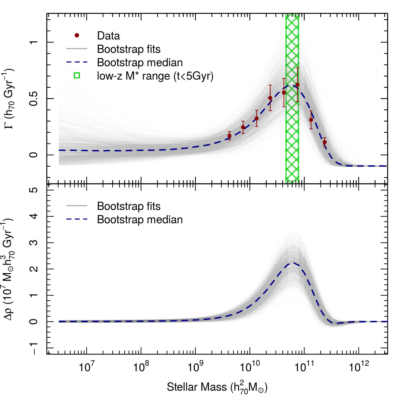
Figure 4: The GSMF average growth function across lookback times $t\in\left[0.2,11.0\right]$, shown in fractional growth ($\Gamma$; top) and in mass density ($\rho$; bottom). The distribution, which is calculated as in Equation 1, demonstrates the average expected growth of the Schechter function number density assuming a uniform growth rate over the entire lookback window. The grey lines show the distribution as calculated from the ratio of each of the 1001 bootstrap realisations shown in bins $1$ and $15$ of Figure 1, with significant transparency. The red points show the ratio of the data in these bins, for the mutually spanned mass range. The blue dashed line is the median of all the bootstrap realisations. The distribution shows that, across this range of lookback times, the average growth per Gyr as been restricted almost entirely to the high-mass end of the Schechter function; around $M^{\star}$. The low-mass end of the Schechter function shows no significant growth (or loss). At the high-mass end the function converges to the limiting value of $-(t_{1}-t_{2})^{-1}\approx-0.1$.

We opt to use bins $1$ ($t_{2}\approx 0.61h_{70}^{-1}{\rm Gyr}$) and $15$ ($t_{1}\approx 10.8h_{70}^{-1}{\rm Gyr}$) to define the growth function, as they span the widest range of lookback time where the low-mass component is not rapidly evolving in normalisation (see Figure 2). Importantly, however, we note that this definition therefore requires significant extrapolation of the bin $15$ Schechter fits, well below the lower mass limit of the data in this bin.

Our average growth function, returned from the individual bootstrap fits to the data, is shown in the upper panel of Figure 4, and the average growth of $\rho_{\star}$ is shown in the lower panel. In both panels we can see a summary of our main conclusion about the evolution of the GSMF; it shows that there is essentially no change in either the mass or number density of the low-mass end of the GSMF over the last $11\,h^{-1}_{70}{\rm Gyr}$ while the high-mass end the GSMF exhibits strong growth which peaks at $\Gamma\approx 0.65\,h_{70}^{-1}{\rm Gyr}$, and $\Delta\rho_{\star}\approx 2\times 10^{7}M_{\odot}h^{3}_{70}{\rm Gyr}^{-1}$, and is centered on $M^{\star}$. At the highest masses the growth function $\Gamma$ converges on its asymptote value, as the exponential tail of the low-z mass function beats its compatriot to 0.

The observed stellar mass growth function essentially describes the integrated effect of all galaxy stellar mass growth/loss/redistribution mechanisms over the $11\,h^{-1}_{70}{\rm Gyr}$s spanned by the growth function definition. This would include, but is of course not limited too:

• growth due to star-formation from all sources (e.g. secular, merger-driven, etc), and how the star-formation rate varies over time;

• mass lost due to stellar evolution, and how this stellar evolution changes with stellar population evolution; and

• mass lost to the intragroup/intracluster/intergalactic medium due to stripping/merger events.

Modelling this complex evolution of mass in the universe is a significant task, and would require comprehensive modelling of (at least) each of the items listed above. Rather than attempt to undertake this task, we instead opt to present our observed mass redistribution function as an additional observable that may be of interest to the community, and leave this comprehensive modelling for the future.

As an observable, our growth function suggests that the assembly of stellar mass over the last $\sim 11h_{70}^{-1}{\rm Gyr}$ has involved an interplay between the various stellar mass growth/destruction/redistribution mechanisms, such that no net loss in mass density occurs at any point in the mass function. As such, this growth function may be verifiable/falsifiable using future simulations and surveys that endeavour to explore the integrated properties of mass evolution. To this end, ongoing and upcoming surveys which will allow the construction of high-fidelity catalogues of group-scale environments will be invaluable. Surveys such as the Deep Extragalactic VIsible Legacy Survey (DEVILS; Davies et. al., 2018) and the Wide Area VISTA Extragalactic Survey (WAVES; Driver et al., 2016a) will be able to estimate the integrated redistribution of mass in a wide range of environments, and will be ideal for this purpose.

This assumes, however, that the true stellar mass growth in the universe varies smoothly. Fortunately, we can simply test whether our observed average growth function is indeed a reasonable representation of the observed mass function, and mass density, at each epoch. We do this simply by using the average growth model to define a simple model GSMF at time $t_{i}$ as:

$$\phi_{{\rm m},i}=\phi_{1}\left[1+\Gamma\left(t_{1}-t_{i}\right)\right].$$ (3)

To demonstrate the surprising amount of similarity that this simple model demonstrates to both the data and our best-fit regressed Schechter functions, we reproduce Figure 1 in Figure 5, except now showing lines for the median bootstrap model, the best-fit regressed model, and the simple constant-growth model alongside one-another. The figure demonstrates that the three models are indeed consistent with each-other, differing most significantly in the overall Schechter normalisation (where the red bootstrap model lines at each epoch trace variations in large scale structure).

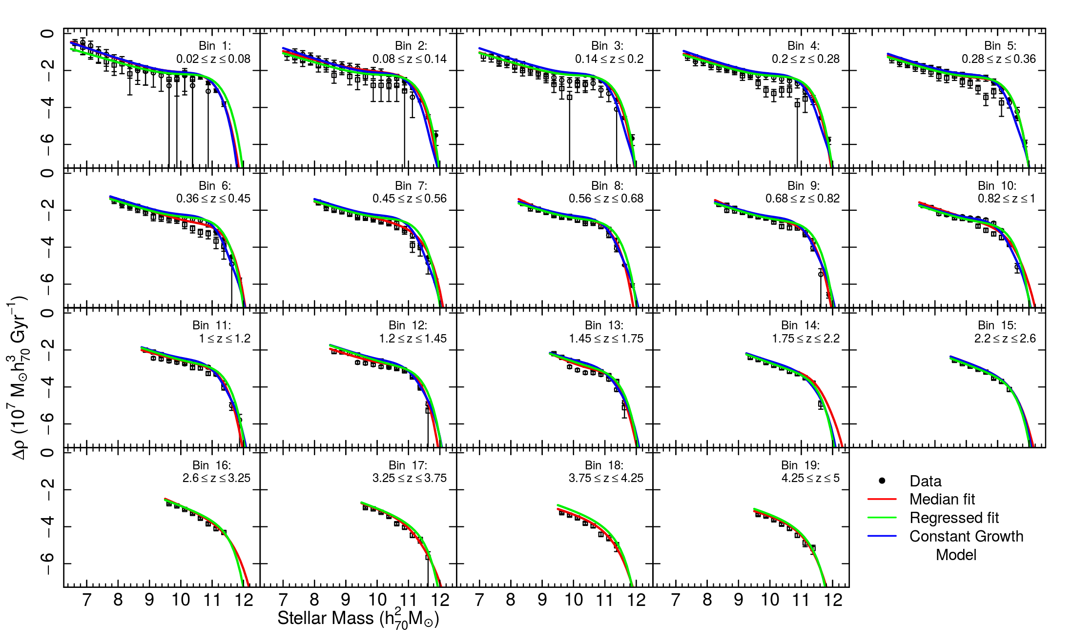
Figure 5: Difference between the three main model types discussed in this work. In each bin, the data are shown in black (reproduced from Figure 1), the weighted median of all bootstrap realisations is shown in red, the model returned from our best fit regressions (see Figure 2) is shown in green, and the model returned by our constant growth model is shown in blue (not shown in bins beyond where the model was defined). At all epochs these fits are essentially consistent.

We then use these simply modelled GSMFs to calculate a model stellar mass density at every epoch, $\rho^{m}_{\star}$, and compare these values to our observed evolution of the stellar mass density parameter $\rho_{\star}$. These results are shown in Figure 6, where we reproduce the bottom left panel of Figure 2, except in this instance we show the mass density curves derived by our regressed Schechter function parameters, rather than the observations themselves (as we did in Figure 2). We then overlay the mass density growth returned by our simple constant growth model, defined in the same way as above, except that in the figure we use the regression values at bins $1$ and $15$ to define a growth function $\Gamma$, rather than the bootstrap fits. This allows us to directly compare how the constant growth model compares to our regression fits, which make-up our best-fitting GSMFs at each epoch.

In the figure, we can see that our regressed parameters are entirely consistent with the literature, even though the uncertainties balloon at the highest redshifts Moreover, we see that the model mass functions $\phi^{\rm r}_{\rm m}$ follow the evolution of the observed data and of the best-fit regression models essentially perfectly over the last $\sim\!11\,h_{70}^{-1}\,{\rm Gyr}$. At the highest redshifts, again, our model does not follow the rapid evolution of the low-mass component and so over-predicts the mass density somewhat. Nonetheless, this result demonstrates that with this strikingly simple model of constant growth of the high-mass component of the GSMF, we are able to reproduce the evolution of the stellar mass density over the vast majority of the evolution history of the universe and that there has been a surprising lack of stocasticity in the overall rate of evolution of the stellar mass density.

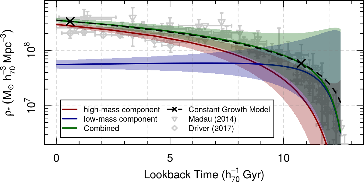
Figure 6: The evolution of the stellar mass density as estimated using our regressed fits and with our simple model of constant high-mass growth in the GSMF. The regressed fits (coloured lines) demonstrate the agreement between our data and the evolution in the literature (grey points), despite the uncertainties on our fits becoming significant at the highest redshifts. Moreover, the simple model of constant mass function growth (black dashed line) is also in excellent agreement with the literature over the last $\sim\!11\,h_{70}^{-1}\,{\rm Gyr}$. At higher-redshift, the simple model is unable to capture the rapid growth of the low-mass component, and so the model over-predicts the stellar mass density, as expected. Here the growth model $\Gamma^{\rm r}$ has been defined using the regressed fits in our bins $1$ and $15$ (shown by the black crosses) so that the green and black lines are directly comparable.

6 Conclusions

In this work we have demonstrated the evolution of Schechter (1976) function parameters over $12.5\,h_{70}^{-1}\,{\rm Gyr}$ using the combined sample of GAMA, G10-COSMOS, and 3D-HST. Using multiple Schechter function fits, we demonstrate that the single component Schechter function is unlikely to produce reliable fits, even out to a redshift of 5. Conversely, the two-component Schechter shows impressive stability of its fitted parameters over the entire redshift range, providing well constrained parameters at essentially all epochs. We explore the evolution of the mass function further by regressing the various parameters such that we achieve a smooth evolution. Our regressed parameters, in our two-component Schechter fits, show little to no evolution of the $M^{\star}$, $\alpha_{i}$, or low-mass $\phi^{\star}$ parameters over time, and are especially stable over the last $\sim\!11.0\,h_{70}^{-1}\,{\rm Gyr}$. Conversely, the high-mass $\phi^{\star}$ parameter shows strong evolution over the same period. The stability of most parameters, coupled with the evolution of the high-mass component’s normalisation parameter, suggests a picture of galaxy evolution where these two components broadly track different mass-evolution mechanisms; the low-mass systems broadly following secular evolution of galaxies, while high-mass systems are constantly being built up through merger processes. At the highest redshifts, the low mass component exhibits somewhat rapid evolution in its normalisation, starting out as the mass-dominant component of the GSMF until it is overtaken at $\sim\!9\,h_{70}^{-1}\,{\rm Gyr}$, when the growing high-mass component becomes the dominant reservoir of mass. We then test whether the build-up of mass over the last $11\,h_{70}^{-1}\,{\rm Gyr}$ is well described by a constant rate of mass growth, finding that this is indeed the case, and that a simple model of the mass function growth is able to perfectly describe the observed evolution of the stellar mass density parameter over the majority of the evolution history of the universe. Nonetheless, we recognise that this mass growth function encodes a highly complex array of mass growth/loss/redistribution mechanisms, and that alone may be only used as a guiding observable in future complex mass-assembly studies. We conclude that upcoming deep and highly complete surveys of group-scale environments, at intermediate to high redshift, will be required in order to determine the mechanisms driving the observed growth of stellar mass.

7 Acknowledgements

We thank the anonymous referee for their thorough reading of our work, and for their many helpful comments. GAMA is a joint European-Australasian project based around a spectroscopic campaign using the Anglo-Australian Telescope. The GAMA input catalogue is based on data taken from the Sloan Digital Sky Survey and the UKIRT Infrared Deep Sky Survey. Complementary imaging of the GAMA regions is being obtained by a number of independent survey programmes including GALEX MIS, VST KiDS, VISTA VIKING, WISE, Herschel-ATLAS, GMRT and ASKAP providing UV to radio coverage. GAMA is funded by the STFC (UK), the ARC (Australia), the AAO and the participating institutions. The GAMA website is http://www.gama-survey.org/. Based on observations made with ESO Telescopes at the La Silla Paranal Observatory under programme ID 179.A-2004. This work uses photometric data measured using lambdar (Wright, 2016), and higher order data products from SEDs measured using magphys (da Cunha & Charlot, 2011). Figures were made with the help of the magicaxis and celestial packages (Robotham, 2016a, b) packages in r (R Core Team, 2015).

Appendix A Fit results & regression functions

Table 1: Best fit single-component Schechter function parameters, and $\chi_{\rm r}^{2}$ values, in each redshift bin. Uncertainties show the asymmetric 1$\sigma$ quantiles on each parameter.

Bin	$M^{\star}$	$\alpha_{1}$	$\phi^{\star}_{1}$	$\rho_{\star}$	$\chi_{\rm r}^{2}$
1	$10.86^{+0.056}_{-0.039}$	$-1.134^{+0.033}_{-0.067}$	$-2.491^{+0.1}_{-0.128}$	$8.419^{+0.083}_{-0.089}$	$1.129_{-0.638}^{+0.972}$
2	$10.934^{+0.056}_{-0.063}$	$-1.172^{+0.14}_{-0.115}$	$-2.471^{+0.118}_{-0.146}$	$8.51^{+0.054}_{-0.059}$	$1.089_{-0.416}^{+0.612}$
3	$10.918^{+0.052}_{-0.06}$	$-1.066^{+0.209}_{-0.127}$	$-2.471^{+0.096}_{-0.127}$	$8.449^{+0.053}_{-0.055}$	$2.654_{-0.640}^{+1.110}$
4	$10.947^{+0.029}_{-0.042}$	$-1.133^{+0.148}_{-0.096}$	$-2.538^{+0.067}_{-0.064}$	$8.443^{+0.037}_{-0.04}$	$2.461_{-0.668}^{+0.944}$
5	$10.994^{+0.028}_{-0.044}$	$-1.131^{+0.195}_{-0.106}$	$-2.614^{+0.067}_{-0.064}$	$8.409^{+0.043}_{-0.049}$	$2.739_{-0.805}^{+1.418}$
6	$11.101^{+0.022}_{-0.028}$	$-1.282^{+0.124}_{-0.065}$	$-2.953^{+0.048}_{-0.047}$	$8.247^{+0.037}_{-0.053}$	$2.743_{-0.772}^{+1.379}$
7	$11.139^{+0.033}_{-0.028}$	$-1.387^{+0.025}_{-0.025}$	$-3.181^{+0.094}_{-0.091}$	$8.129^{+0.061}_{-0.071}$	$0.775_{-0.319}^{+0.790}$
8	$10.956^{+0.044}_{-0.033}$	$-1.35^{+0.03}_{-0.042}$	$-2.967^{+0.119}_{-0.169}$	$8.125^{+0.076}_{-0.101}$	$2.185_{-0.664}^{+0.823}$
9	$10.985^{+0.048}_{-0.019}$	$-1.372^{+0.018}_{-0.023}$	$-3.059^{+0.082}_{-0.098}$	$8.097^{+0.062}_{-0.075}$	$2.008_{-0.649}^{+0.837}$
10	$11.212^{+0.073}_{-0.058}$	$-1.486^{+0.024}_{-0.029}$	$-3.334^{+0.097}_{-0.105}$	$8.124^{+0.061}_{-0.069}$	$3.523_{-1.135}^{+1.653}$
11	$11.082^{+0.048}_{-0.039}$	$-1.319^{+0.024}_{-0.023}$	$-3.203^{+0.075}_{-0.081}$	$8.006^{+0.057}_{-0.065}$	$2.630_{-0.763}^{+1.078}$
12	$11.081^{+0.06}_{-0.035}$	$-1.297^{+0.031}_{-0.035}$	$-3.256^{+0.08}_{-0.083}$	$7.947^{+0.056}_{-0.063}$	$2.987_{-1.209}^{+2.338}$
13	$11.167^{+0.062}_{-0.055}$	$-1.398^{+0.069}_{-0.077}$	$-3.498^{+0.097}_{-0.134}$	$7.844^{+0.052}_{-0.055}$	$6.571_{-2.919}^{+3.913}$
14	$11.495^{+0.005}_{-0.131}$	$-1.528^{+0.023}_{-0.018}$	$-3.74^{+0.091}_{-0.092}$	$7.983^{+0.077}_{-0.077}$	$0.271_{-0.150}^{+0.286}$
15	$11.498^{+0.002}_{-0.234}$	$-1.664^{+0.094}_{-0.037}$	$-4.022^{+0.331}_{-0.07}$	$7.896^{+0.035}_{-0.044}$	$1.235_{-0.646}^{+0.969}$
16	$11.471^{+0.029}_{-0.256}$	$-1.726^{+0.022}_{-0.012}$	$-4.329^{+0.181}_{-0.069}$	$7.613^{+0.053}_{-0.048}$	$4.006_{-1.867}^{+2.749}$
17	$11.5^{+0.00}_{-0.011}$	$-1.78^{+0.00}_{-0.009}$	$-4.623^{+0.064}_{-0.104}$	$7.459^{+0.099}_{-0.075}$	$5.835_{-2.561}^{+2.818}$
18	$11.122^{+0.378}_{-0.503}$	$-1.648^{+0.272}_{-0.133}$	$-4.453^{+0.517}_{-0.46}$	$7.051^{+0.164}_{-0.159}$	$2.547_{-1.331}^{+1.692}$
19	$11.116^{+0.027}_{-0.012}$	$-1.634^{+0.029}_{-0.042}$	$-4.496^{+0.036}_{-0.08}$	$7.006^{+0.047}_{-0.052}$	$1.861_{-0.888}^{+1.555}$

Table 2: Best fit 2-component Schechter function parameters, and median $\chi_{\rm r}^{2}$ values, in each redshift bin. Uncertainties show the asymmetric 1$\sigma$ quantiles on each parameter.

Bin	$M^{\star}$	$\alpha_{1}$	$\alpha_{2}$	$\phi^{\star}_{1}$	$\phi^{\star}_{2}$	$\rho_{\star}$	$\chi_{\rm r}^{2}$
1	$10.68^{+0.079}_{-0.077}$	$-0.515^{+0.206}_{-0.319}$	$-1.517^{+0.179}_{-0.204}$	$-2.304^{+0.117}_{-0.12}$	$-3.13^{+0.335}_{-0.506}$	$8.455^{+0.082}_{-0.093}$	$0.531_{-0.275}^{+0.512}$
2	$10.8^{+0.044}_{-0.043}$	$-0.612^{+0.133}_{-0.288}$	$-1.457^{+0.101}_{-0.11}$	$-2.377^{+0.093}_{-0.103}$	$-3.037^{+0.205}_{-0.711}$	$8.526^{+0.05}_{-0.065}$	$0.836_{-0.329}^{+0.728}$
3	$10.819^{+0.033}_{-0.028}$	$-0.646^{+0.103}_{-0.142}$	$-1.507^{+0.049}_{-0.117}$	$-2.39^{+0.06}_{-0.071}$	$-3.452^{+0.191}_{-0.373}$	$8.457^{+0.046}_{-0.049}$	$1.982_{-0.641}^{+0.847}$
4	$10.837^{+0.019}_{-0.014}$	$-0.645^{+0.017}_{-0.082}$	$-1.516^{+0.013}_{-0.104}$	$-2.456^{+0.047}_{-0.047}$	$-3.384^{+0.169}_{-0.357}$	$8.431^{+0.034}_{-0.038}$	$1.780_{-0.534}^{+0.754}$
5	$10.88^{+0.013}_{-0.026}$	$-0.55^{+0.117}_{-0.043}$	$-1.536^{+0.035}_{-0.054}$	$-2.555^{+0.038}_{-0.041}$	$-3.4^{+0.125}_{-0.184}$	$8.388^{+0.038}_{-0.038}$	$1.592_{-0.558}^{+1.207}$
6	$10.967^{+0.014}_{-0.017}$	$-0.487^{+0.052}_{-0.01}$	$-1.586^{+0.095}_{-0.019}$	$-2.936^{+0.048}_{-0.072}$	$-3.541^{+0.268}_{-0.17}$	$8.192^{+0.05}_{-0.047}$	$1.561_{-0.574}^{+1.294}$
7	$11.065^{+0.079}_{-0.067}$	$-0.487^{+0.055}_{-0.046}$	$-1.423^{+0.025}_{-0.118}$	$-3.632^{+0.409}_{-{\rm Inf}}$	$-3.241^{+0.122}_{-0.247}$	$8.115^{+0.078}_{-0.079}$	$0.904_{-0.385}^{+0.705}$
8	$10.805^{+0.039}_{-0.021}$	$-0.782^{+0.136}_{-0.133}$	$-1.98^{+0.413}_{-0.02}$	$-2.659^{+0.104}_{-0.148}$	$-4.205^{+0.922}_{-0.127}$	$8.508^{+4.728}_{-0.299}$	$2.561_{-0.661}^{+0.810}$
9	$10.881^{+0.04}_{-0.087}$	$-0.858^{+0.062}_{-0.154}$	$-1.838^{+0.254}_{-0.126}$	$-2.84^{+0.136}_{-0.172}$	$-3.977^{+0.507}_{-0.356}$	$8.204^{+0.152}_{-0.095}$	$2.495_{-0.792}^{+1.078}$
10	$11.06^{+0.191}_{-0.126}$	$-0.986^{+0.1}_{-0.114}$	$-1.591^{+0.091}_{-0.209}$	$-3.321^{+0.332}_{-{\rm Inf}}$	$-3.532^{+0.186}_{-0.291}$	$8.138^{+0.064}_{-0.062}$	$3.799_{-1.175}^{+1.804}$
11	$10.862^{+0.064}_{-0.074}$	$-0.522^{+0.177}_{-0.155}$	$-1.488^{+0.043}_{-0.05}$	$-3.07^{+0.102}_{-0.092}$	$-3.409^{+0.092}_{-0.121}$	$8.025^{+0.053}_{-0.066}$	$2.564_{-0.700}^{+1.184}$
12	$10.857^{+0.039}_{-0.052}$	$-0.525^{+0.102}_{-0.097}$	$-1.525^{+0.038}_{-0.111}$	$-3.049^{+0.127}_{-0.09}$	$-3.589^{+0.105}_{-0.151}$	$7.974^{+0.058}_{-0.062}$	$2.361_{-0.954}^{+1.984}$
13	$10.896^{+0.134}_{-0.131}$	$-0.36^{+0.511}_{-0.552}$	$-1.653^{+0.093}_{-0.347}$	$-3.295^{+0.185}_{-0.145}$	$-3.785^{+0.244}_{-0.194}$	$7.891^{+0.109}_{-0.063}$	$6.656_{-3.263}^{+4.003}$
14	$11.041^{+0.248}_{-0.075}$	$-0.351^{+0.041}_{-0.027}$	$-1.589^{+0.045}_{-0.073}$	$-3.478^{+0.158}_{-0.499}$	$-3.648^{+0.099}_{-0.107}$	$7.98^{+0.072}_{-0.075}$	$0.342_{-0.185}^{+0.301}$
15	$11.075^{+0.098}_{-0.098}$	$-0.336^{+0.064}_{-0.074}$	$-1.58^{+0.033}_{-0.048}$	$-4.039^{+0.277}_{-0.389}$	$-3.62^{+0.062}_{-0.094}$	$7.846^{+0.045}_{-0.058}$	$1.008_{-0.573}^{+1.014}$
16	$11.306^{+0.085}_{-0.126}$	$-0.734^{+0.202}_{-0.138}$	$-1.731^{+0.061}_{-0.048}$	$-$	$-4.169^{+0.185}_{-0.145}$	$7.667^{+0.06}_{-0.065}$	$2.033_{-1.013}^{+1.412}$
17	$10.884^{+0.426}_{-0.2}$	$-0.154^{+0.457}_{-0.656}$	$-1.557^{+0.185}_{-0.199}$	$-$	$-3.862^{+0.301}_{-0.549}$	$7.358^{+0.127}_{-0.078}$	$4.491_{-2.149}^{+2.901}$
18	$10.777^{+0.19}_{-0.167}$	$0.056^{+0.312}_{-0.365}$	$-1.484^{+0.119}_{-0.136}$	$-4.787^{+0.29}_{-{\rm Inf}}$	$-4.005^{+0.197}_{-0.268}$	$7.048^{+0.08}_{-0.087}$	$2.782_{-1.652}^{+2.735}$
19	$10.71^{+0.156}_{-0.18}$	$0.168^{+0.295}_{-0.277}$	$-1.437^{+0.14}_{-0.12}$	$-4.846^{+0.331}_{-{\rm Inf}}$	$-4.02^{+0.209}_{-0.221}$	$6.918^{+0.078}_{-0.069}$	$3.038_{-1.730}^{+3.205}$

Fit Type	Parmeter	$A_{0}$	$A_{1}$	$A_{2}$
	$M^{\star}$	$10.791\pm 0.050$	$0.558\pm 0.056$	$-0.102\pm 0.013$
Single	$\alpha$	$-1.160\pm 0.060$	$-0.274\pm 0.067$	$0.028\pm 0.015$
	$\phi^{\star}$	$-2.455\pm 0.069$	$-0.883\pm 0.103$	$0.093\pm 0.022$
	$\rho_{\star}$	$8.433\pm 0.046$	$-0.273\pm 0.063$	$-0.005\pm 0.014$
	$M^{\star}$	$10.831\pm 0.037$	$0.153\pm 0.096$	$-0.033\pm 0.028$
	$\alpha_{1}$	$-0.579\pm 0.063$	$0.048\pm 0.115$	$0.022\pm 0.039$
Two Comp.	$\alpha_{2}$	$-1.489\pm 0.038$	$-0.087\pm 0.053$	$0.016\pm 0.014$
	$\phi^{\star}_{1}$	$-2.312\pm 0.032$	$-0.658\pm 0.119$	$0.016\pm 0.066$
	$\phi^{\star}_{2}$	$-3.326\pm 0.099$	$-0.158\pm 0.103$	$-0.002\pm 0.024$
	$\rho_{\star,1}$	$8.452\pm 0.025$	$-0.554\pm 0.091$	$-0.007\pm 0.050$
	$\rho_{\star,2}$	$7.678\pm 0.079$	$0.088\pm 0.108$	$-0.050\pm 0.026$
	$\rho_{\star,c}$	$8.449\pm 0.039$	$-0.271\pm 0.062$	$-0.012\pm 0.015$

Table 3: Regression functions displayed in Figure 2 for both single and two-component fits. Fits are quadratic in redshift, where the $A_{i}$ coefficient applies to the $i^{\rm th}$ power of $z$.

References

- Andrews et al. (2017) Andrews S. K., Driver S. P., Davies L. J. M., Kafle P. R., Robotham A. S. G., Wright A. H., 2017, MNRAS, 464, 1569
- Baldry et al. (2008) Baldry I. K., Glazebrook K., Driver S. P., 2008, MNRAS, 388, 945
- Baldry et al. (2012) Baldry I. K., et al., 2012, MNRAS, 421, 621
- Baldry et al. (2018) Baldry I. K., et al., 2018, MNRAS, 474, 3875
- Bell et al. (2003) Bell E. F., McIntosh D. H., Katz N., Weinberg M. D., 2003, ApJS, 149, 289
- Brammer et al. (2012) Brammer G. B., et al., 2012, ApJS, 200, 13
- Bridge et al. (2010) Bridge C. R., Carlberg R. G., Sullivan M., 2010, ApJ, 709, 1067
- Bruzual & Charlot (2003) Bruzual G., Charlot S., 2003, MNRAS, 344, 1000
- Byrd et al. (1995) Byrd R. H., Lu P., Nocedal J., Zhu C., 1995, SIAM J. Sci. Comput., 16, 1190
- Chabrier (2003) Chabrier G., 2003, PASP, 115, 763
- Charlot & Fall (2000) Charlot S., Fall S. M., 2000, ApJ, 539, 718
- Cole et al. (2001) Cole S., et al., 2001, MNRAS, 326, 255
- Croom et al. (2005) Croom S. M., et al., 2005, MNRAS, 356, 415
- Davidzon et al. (2017) Davidzon I., et al., 2017, preprint, (arXiv:1701.02734)
- Davies et al. (2015) Davies L. J. M., et al., 2015, MNRAS, 452, 616
- Davies et. al. (2018) Davies et. al. 2018, in preparation
- Donley et al. (2012) Donley J. L., et al., 2012, ApJ, 748, 142
- Driver et al. (2009) Driver S. P., et al., 2009, Astronomy and Geophysics, 50, 050000
- Driver et al. (2011) Driver S. P., et al., 2011, MNRAS, 413, 971
- Driver et al. (2016a) Driver S. P., Davies L. J., Meyer M., Power C., Robotham A. S. G., Baldry I. K., Liske J., Norberg P., 2016a, The Universe of Digital Sky Surveys, 42, 205
- Driver et al. (2016b) Driver S. P., et al., 2016b, MNRAS, 455, 3911
- Driver et al. (2017) Driver S. P., et al., 2017, preprint, (arXiv:1710.06628)
- Drory & Alvarez (2008) Drory N., Alvarez M., 2008, ApJ, 680, 41
- Fontana et al. (2006) Fontana A., et al., 2006, A&A, 459, 745
- Gawiser et al. (2006) Gawiser E., et al., 2006, ApJS, 162, 1
- Giavalisco et al. (2004) Giavalisco M., et al., 2004, ApJ, 600, L93
- Grazian et al. (2015) Grazian A., et al., 2015, A&A, 575, A96
- Grogin et al. (2011) Grogin N. A., et al., 2011, ApJS, 197, 35
- Ilbert et al. (2013) Ilbert O., et al., 2013, A&A, 556, A55
- Kelvin et al. (2014) Kelvin L. S., et al., 2014, MNRAS, 439, 1245
- Koekemoer et al. (2011) Koekemoer A. M., et al., 2011, ApJS, 197, 36
- Leja et al. (2015) Leja J., van Dokkum P. G., Franx M., Whitaker K. E., 2015, ApJ, 798, 115
- Madau & Dickinson (2014) Madau P., Dickinson M., 2014, ARA&A, 52, 415
- Marchesini et al. (2009) Marchesini D., van Dokkum P. G., Förster Schreiber N. M., Franx M., Labbé I., Wuyts S., 2009, ApJ, 701, 1765
- Moffett et al. (2016) Moffett A. J., et al., 2016, MNRAS, 457, 1308
- Momcheva et al. (2016) Momcheva I. G., et al., 2016, ApJS, 225, 27
- Moster et al. (2010) Moster B. P., Somerville R. S., Maulbetsch C., van den Bosch F. C., Macciò A. V., Naab T., Oser L., 2010, ApJ, 710, 903
- Muzzin et al. (2013) Muzzin A., et al., 2013, ApJ, 777, 18
- Obreschkow et al. (2018) Obreschkow D., Murray S. G., Robotham A. S. G., Westmeier T., 2018, MNRAS, 474, 5500
- R Core Team (2015) R Core Team 2015, R: A Language and Environment for Statistical Computing. R Foundation for Statistical Computing, Vienna, Austria, https://www.R-project.org/
- Robotham (2016b) Robotham A. S. G., 2016b, Celestial: Common astronomical conversion routines and functions, Astrophysics Source Code Library (ascl:1602.011)
- Robotham (2016a) Robotham A. S. G., 2016a, magicaxis: Pretty scientific plotting with minor-tick and log minor-tick support, Astrophysics Source Code Library (ascl:1604.004)
- Robotham et al. (2014) Robotham A. S. G., et al., 2014, MNRAS, 444, 3986
- Rodríguez-Puebla et al. (2017) Rodríguez-Puebla A., Primack J. R., Avila-Reese V., Faber S. M., 2017, MNRAS, 470, 651
- Schechter (1976) Schechter P., 1976, ApJ, 203, 297
- Scoville et al. (2007) Scoville N., et al., 2007, ApJS, 172, 1
- Seymour et al. (2008) Seymour N., et al., 2008, MNRAS, 386, 1695
- Skelton et al. (2014) Skelton R. E., et al., 2014, ApJS, 214, 24
- Song et al. (2016) Song M., et al., 2016, ApJ, 825, 5
- Tomczak et al. (2014) Tomczak A. R., et al., 2014, ApJ, 783, 85
- Wright (2016) Wright A. H., 2016, LAMBDAR: Lambda Adaptive Multi-Band Deblending Algorithm in R, Astrophysics Source Code Library (ascl:1604.003)
- Wright et al. (2016) Wright A. H., et al., 2016, MNRAS,
- Wright et al. (2017) Wright A. H., et al., 2017, MNRAS, 470, 283
- Zheng et al. (2007) Zheng Z., Coil A. L., Zehavi I., 2007, ApJ, 667, 760
- da Cunha & Charlot (2011) da Cunha E., Charlot S., 2011, MAGPHYS: Multi-wavelength Analysis of Galaxy Physical Properties, Astrophysics Source Code Library (ascl:1106.010)
- da Cunha et al. (2008) da Cunha E., Charlot S., Elbaz D., 2008, MNRAS, 388, 1595