Beyond the Central Limit Theorem: Universal and Non-universal Simulations of Random Variables by General Mappings

Abstract

Motivated by the Central Limit Theorem, in this paper, we study both universal and non-universal simulations of random variables with an arbitrary target distribution $Q_{Y}$ by general mappings, not limited to linear ones (as in the Central Limit Theorem). We derive the fastest convergence rate of the approximation errors for such problems. Interestingly, we show that for discontinuous or absolutely continuous $P_{X}$, the approximation error for the universal simulation is almost as small as that for the non-universal one; and moreover, for both universal and non-universal simulations, the approximation errors by general mappings are strictly smaller than those by linear mappings. Furthermore, we also generalize these results to simulation from Markov processes, and simulation of random elements (or general random variables).

Index terms: Universal simulation, random number generation, absolutely continuous distribution, total variation distance, Kolmogorov-Smirnov distance, squeezing periodic functions

2000 Mathematics subject classification: Primary 65C10; Secondary 60F05;62E20;62E17

1 Introduction

The Central Limit Theorem (CLT) states that for a sequence of i.i.d. real-valued random variables $X^{n}\sim P_{X}^{n}$, the normalized sum $\frac{1}{\mathrm{Var}(X)\sqrt{n}}\sum_{i=1}^{n}\left(X_{i}-\mathbb{E}\left[X\right]\right)$ converges in distribution to a standard Gaussian random variable as $n$ goes to infinity. This implies that an $n$-dimensional i.i.d. random vector $X^{n}$ can be used to simulate a standard Gaussian random variable $Y$ by the normalized sum so that the approximation error asymptotically vanishes under the Kolmogorov–Smirnov distance. Moreover, from the Berry-Esseen theorem [1, Sec. XVI.5], the approximation error vanishes in a rate of $\frac{1}{\sqrt{n}}$. Note that here, the distribution $P_{X}$ of $X$ is arbitrary, and given the mean and variance, the linear function is independent of $P_{X}$. Hence such a linear function can be considered as a universal linear function. The corresponding simulation problem can be considered as being universal. In this paper, we consider general universal simulation problems, in which general simulation functions, not limited to linear ones, are allowed. We are interested in the following question: What is the optimal convergence rate for such universal simulation problems? To know how important the knowledge of the distribution $P_{X}$ is in a simulation, we are also interested in the optimal convergence rate for non-universal simulation problems (in which $P_{X}$ is known). Is the optimal convergence rate for universal simulation as fast as, or strictly slower than, that for non-universal simulation?

The CLT is about universal simulation of a continuous random variable (more specifically, a Gaussian random variable). In addition to simulation of continuous random variables, there are a large number of works that consider universal simulation of a sequence of discrete (or atomic) random variables from another sequence of discrete random variables. In 1951, von Neumann [2] described a procedure for exactly generating a sequence of independent and identically distributed (i.i.d.) unbiased random coins from a sequence of i.i.d. biased random coins with an unknown distribution. To obtain unbiased outputs, two pairs of bits $(0,1)$ and $(1,0)$ (which have the same empirical distribution) are mapped to $0$ and $1$, respectively, and $(0,0)$ and $(1,1)$ are discarded. Elias [3] and Blum [4] considered a more general situation in which the process of the repeated coin tosses is subject to an unknown Markov process, instead of a traditional i.i.d. process, and then studied the efficiency of such a procedure measured according to the expected number of output coins per input coin. Knuth and Yao [5], Roche [6], Abrahams [7], and Han and Hoshi [8] considered another general simulation problem in which an arbitrary target distribution is generated by using a unbiased or biased $M$-coin (i.e., an $M$-sided coin) but with a known distribution. They showed that the minimum expected number of coin tosses required to generate the target distribution can be expressed in terms of the ratio of the entropy of the target distribution to that of the seed distribution. In all of the works above [2, 3, 4, 5, 6, 7, 8], simulators are defined as functions that map a variable-length input sequence to a fixed-length output sequence. Hence, to produce an output symbol, arbitrarily long delay or waiting time may be required.

To reduce delay, a direction of generalizing the random number generation problem is to require that an output must be generated for every $k$ bits input from a unbiased or biased coin, for any fixed $k$, but at the same time, relax the requirement of exact generation to that of approximate generation. That is, we may require only that the target distribution should be generated approximately within a nonzero but arbitrarily small tolerance in terms of some suitable distance measures such as the total variation distance or divergences. Such a problem in the asymptotic context with known seed and target distributions has been formulated and studied by Han and Verdú [9]; its inverse problem has been investigated by Vembu and Verdú [10]; and a general version of these problems —– generating an i.i.d. sequence from another i.i.d. sequence with arbitrary known seed and target distributions —– has been studied in [11, 12, 13].

All of the works above only considered simulating a sequence of discrete random variables from another sequence of discrete random variables. In contrast, in this paper we consider approximately generating an arbitrary random variable (or a random element) from a sequence of random variables (or another random element) with arbitrary but unknown seed distribution.

Besides the CLT, this work is also motivated by the following questions. 1) Given a distribution $Q_{Y}$ (defined on $\left(\mathbb{R},\mathcal{B}_{\mathbb{R}}\right)$), is there a measurable function $f:\mathbb{R}\to\mathbb{R}$ such that $P_{f(X)}=Q_{Y}$ for all absolutely continuous distribution $P_{X}$? Here $P_{f(X)}$ is the distribution of the image $f(X)$ induced by $P_{X}$ and the function $f$. 2) Given $Q_{Y}$, is there a sequence of measurable functions $f_{k}:\mathbb{R}\to\mathbb{R}$ such that $P_{f_{k}(X)}\to Q_{Y}$ as $k\to\infty$ (under the total variation distance or other distance measures) for all absolutely continuous distribution $P_{X}$? By some simple derivations, it is easy to show that the answer to the first question is negative. So it is intuitive to conjecture the answer to the second one is also negative, since the second question reduces to the first question if the limit of the sequence $\left\{f_{k}\right\}$ is set to the function $f$. However, the results in this paper show that this conjecture is not right, since the limit of the optimal sequence $\left\{f_{k}\right\}$ does not exist and hence these two questions are not equivalent. Interestingly, we show that the answer to the second question is positive.

1.1 Problem Formulation

Before formulating our problem, we first introduce two statistical distances. For an arbitrary measurable space $\left(\Omega,\mathcal{B}_{\Omega}\right)$, we use $\mathcal{P}(\Omega,\mathcal{B}_{\Omega})$ to denote the set of all the probability measures (a.k.a. distributions) defined on $\left(\Omega,\mathcal{B}_{\Omega}\right)$. Given an arbitrary measurable space $\left(\Omega,\mathcal{B}_{\Omega}\right)$, the total variation (TV) distance between two probability measures $P,Q\in\mathcal{P}(\Omega,\mathcal{B}_{\Omega})$ is defined as

$$\left|P-Q\right|_{\mathrm{TV}} =\sup_{A\in\mathcal{B}_{\Omega}}\left|P(A)-Q(A)\right|.$$

The Kolmogorov–Smirnov (KS) distance between two probability measures $P,Q\in\mathcal{P}(\mathbb{R},\mathcal{B}_{\mathbb{R}})$ is defined as

$$\left|P-Q\right|_{\mathrm{KS}} =\sup_{x\in\mathbb{R}}\left|F(x)-G(x)\right|,$$

where $F$ and $G$ respectively denote the CDFs (cumulative distribution functions) of $P$ and $Q$. For $P,Q\in\mathcal{P}(\mathbb{R},\mathcal{B}_{\mathbb{R}})$, we have

$$0\leq\left|P-Q\right|_{\mathrm{KS}}\leq\left|P-Q\right|_{\mathrm{TV}},$$

since $\left|P-Q\right|_{\mathrm{KS}}=\sup_{A\in\mathcal{I}}\left|P(A)-Q(A)\right|$ with $\mathcal{I}:=\left\{(-\infty,y]:\>y\in\mathbb{R}\right\}\subseteq\mathcal{B}_{\mathbb{R}}$. Furthermore, both $\left|P-Q\right|_{\mathrm{KS}}$ and $\left|P-Q\right|_{\mathrm{TV}}$ are metrics, and hence $\left|P-Q\right|_{\mathrm{KS}}=0\;\Longleftrightarrow\;P=Q$ and $\left|P-Q\right|_{\mathrm{TV}}=0\;\Longleftrightarrow\;P=Q$.

Based on these two distances, we next formulate our problem. In this paper, we consider the following problem: When we use an $n$-dimensional real-valued random vector $X^{n}$ with distribution $P_{X^{n}}$ to generate a real-valued random variable $Y$ by a function $y=f(x^{n})$ so that its distribution is approximately $Q_{Y}$, what is the fastest convergence speed of the approximation error over all functions $f$ as $n$ tends to infinity? Here the approximation error is measured by the TV distance or the KS distance. We term the Borel space $\left(\mathbb{R}^{n},\mathcal{B}_{\mathbb{R}^{n}}\right)$ of $X^{n}$ as the seed space, and the Borel space $\left(\mathbb{R},\mathcal{B}_{\mathbb{R}}\right)$ of $Q_{Y}$ as the target space.

Definition 1.1.

Given the seed Borel space $\left(\mathbb{R}^{n},\mathcal{B}_{\mathbb{R}^{n}}\right)$ and the target Borel space $\left(\mathbb{R},\mathcal{B}_{\mathbb{R}}\right)$, a simulator is a measurable function $f:\mathbb{R}^{n}\to\mathbb{R}$.

Given a random vector $X^{n}\sim P_{X^{n}}$ and a target distribution $Q_{Y}$, we want to find an optimal simulator $Y=f(X^{n})$ that minimizes the TV distance or the KS distance between the output distribution $P_{Y}:=P_{X^{n}}\circ f^{-1}$ (the distribution of the output random variable $Y$) and the target distribution $Q_{Y}$. For such a simulation problem, we consider two different scenarios where $P_{X^{n}}$ is respectively known and unknown a priori.

As illustrated in Fig. 1 (a), if the seed distribution $P_{X^{n}}$ is unknown, but the class $\mathcal{P}_{X^{n}}\subseteq\mathcal{P}(\mathbb{R}^{n},\mathcal{B}_{\mathbb{R}^{n}})$ that $P_{X^{n}}$ belongs to is known, we term such simulation problems as (universal) $(\mathcal{P}_{X^{n}},Q_{Y})$-simulation problems. Hence, the simulator $f:\mathbb{R}^{n}\to\mathbb{R}$ in the universal simulation problem may depend on everything including $Q_{X}$ and $\mathcal{P}_{X^{n}}$, but except for $P_{X^{n}}$. That is, it is independent of $P_{X^{n}}$ given $\mathcal{P}_{X^{n}}$. Next we give a mathematical formulation for the universal simulation problem, which avoids ambiguous languages, like “$P_{X^{n}}$ is unknown”.

(a) The universal $(\mathcal{P}_{X^{n}},Q_{Y})$-simulation problem

(b) The non-universal $(P_{X^{n}},Q_{Y})$-simulation problem

Figure 1: Universal and non-universal simulation problems.

Definition 1.2.

A function $g:\mathcal{P}_{X^{n}}\to\mathbb{R}$ is called TV-achievable (resp. KS-achievable) for the universal $(\mathcal{P}_{X^{n}},Q_{Y})$-simulation, if there exists a sequence of simulators $\left\{f_{n,k}\right\}_{k=1}^{\infty}$ such that

$$\limsup_{k\to\infty}\left|P_{Y_{n,k}}-Q_{Y}\right|_{\theta}\leq g(P_{X^{n}})$$

for all $P_{X^{n}}\in\mathcal{P}_{X^{n}}$, where $P_{Y_{n,k}}:=P_{X^{n}}\circ f_{n,k}^{-1}$ and $\theta=\mathrm{TV}$ (resp. $\theta=\mathrm{KS}$).

Definition 1.3.

The set of TV-achievable (resp. KS-achievable) functions for the universal $(\mathcal{P}_{X^{n}},Q_{Y})$-simulation is defined as

$$\mathcal{E}_{\theta}(\mathcal{P}_{X^{n}},Q_{Y}):=\left\{g:\mathcal{P}_{X^{n}}\to\mathbb{R}\>:g\textrm{ is }\theta\raisebox{0.75pt}{-}\textrm{achievable}\right\}$$

where $\theta=\mathrm{TV}$ (resp. $\theta=\mathrm{KS}$).

According to Lebesgue’s decomposition theorem [14], the distributions of real-valued random variables can be partitioned into three classes: discontinuous distributions (including discrete distributions and mixtures of discrete and continuous distributions), absolutely continuous distributions, and continuous but not absolutely continuous distributions (including singular continuous distributions and mixtures of singular continuous and absolutely continuous distributions). The sets of these distributions are respectively denoted as $\mathcal{P}_{\mathrm{dc}},\mathcal{P}_{\mathrm{ac}}$, and $\mathcal{P}_{\mathrm{c}}\backslash\mathcal{P}_{\mathrm{ac}}$, where $\mathcal{P}_{\mathrm{c}}=\mathcal{P}(\mathbb{R},\mathcal{B}_{\mathbb{R}})\backslash\mathcal{P}_{\mathrm{dc}}$ denotes the set of continuous distributions on $\left(\mathbb{R},\mathcal{B}_{\mathbb{R}}\right)$.

For the i.i.d. case, we define $\mathcal{P}_{X}^{(n)}:=\left\{P_{X}^{n}:P_{X}\in\mathcal{P}_{X}\right\}$. In this paper, we want to characterize $\mathcal{E}_{\theta}(\mathcal{P}_{X}^{(n)},Q_{Y})$ with $\mathcal{P}_{X}$ respectively set to $\mathcal{P}_{\mathrm{dc}},\mathcal{P}_{\mathrm{ac}}$, or $\mathcal{P}_{\mathrm{c}}\backslash\mathcal{P}_{\mathrm{ac}}$. Note that $\mathcal{E}_{\theta}(\mathcal{P}_{X}^{(n)},Q_{Y})$ is an upper set. For brevity, for such sets and a function $g:\mathcal{P}_{X}\to\mathbb{R}$, we denote $\mathcal{E}_{\theta}(\mathcal{P}_{X}^{(n)},Q_{Y})\preceq g$ if there exists a $g^{\prime}\in\mathcal{E}_{\theta}(\mathcal{P}_{X}^{(n)},Q_{Y})$ such that $g^{\prime}(P_{X})\leq g(P_{X}),\forall P_{X}\in\mathcal{P}_{X}$; and $\mathcal{E}_{\theta}(\mathcal{P}_{X}^{(n)},Q_{Y})\succeq g$ if $g^{\prime}(P_{X})\geq g(P_{X}),\forall P_{X}\in\mathcal{P}_{X}$ for all $g^{\prime}\in\mathcal{E}_{\theta}(\mathcal{P}_{X}^{(n)},Q_{Y})$. In addition, $\mathcal{E}_{\theta}(\mathcal{P}_{X}^{(n)},Q_{Y})\asymp g$ if and only if $\mathcal{E}_{\theta}(\mathcal{P}_{X}^{(n)},Q_{Y})\preceq g$ and $\mathcal{E}_{\theta}(\mathcal{P}_{X}^{(n)},Q_{Y})\succeq g$. In general, there does not necessarily exist $g$ such that $\mathcal{E}_{\theta}(\mathcal{P}_{X}^{(n)},Q_{Y})\asymp g$. However, if it exists, then $g(P_{X})=\inf_{g^{\prime}\in\mathcal{E}_{\theta}(\mathcal{P}_{X}^{(n)},Q_{Y})}g^{\prime}(P_{X})$ for $P_{X}\in\mathcal{P}_{X}$.

Similarly, we write $\mathcal{E}_{\theta}(\mathcal{P}_{X}^{(n)},Q_{Y})\mathrel{\dot{\preceq}}g_{n}$ if there exists a $g_{n}^{\prime}\in\mathcal{E}_{\theta}(\mathcal{P}_{X}^{(n)},Q_{Y})$ such that $g_{n}^{\prime}(P_{X})\mathrel{\dot{\leq}}g_{n}(P_{X}),\forall P_{X}\in\mathcal{P}_{X}$; and $\mathcal{E}_{\theta}(\mathcal{P}_{X}^{(n)},Q_{Y})\mathrel{\dot{\succeq}}g$ if $g_{n}^{\prime}(P_{X})\mathrel{\dot{\geq}}g_{n}(P_{X}),\forall P_{X}\in\mathcal{P}_{X}$ for all $g_{n}^{\prime}\in\mathcal{E}_{\theta}(\mathcal{P}_{X}^{(n)},Q_{Y})$. In addition, $\mathcal{E}_{\theta}(\mathcal{P}_{X}^{(n)},Q_{Y})\mathrel{\dot{\asymp}}g_{n}$ if and only if $\mathcal{E}_{\theta}(\mathcal{P}_{X}^{(n)},Q_{Y})\mathrel{\dot{\preceq}}g$ and $\mathcal{E}_{\theta}(\mathcal{P}_{X}^{(n)},Q_{Y})\mathrel{\dot{\succeq}}g$. Furthermore, $\mathcal{E}_{\theta}(\mathcal{P}_{X}^{(n)},Q_{Y})\asymp e^{-\Omega(g_{n})}$ (resp. $\mathcal{E}_{\theta}(\mathcal{P}_{X}^{(n)},Q_{Y})\asymp e^{-\omega(g_{n})}$) if there exists a $g_{n}^{\prime}\in\mathcal{E}_{\theta}(\mathcal{P}_{X}^{(n)},Q_{Y})$ such that $g_{n}^{\prime}(P_{X})=e^{-\Omega(g_{n}(P_{X}))}$ (resp. $g_{n}^{\prime}(P_{X})=e^{-\omega(g_{n}(P_{X}))}$) for all $P_{X}\in\mathcal{P}_{X}$.

Conversely, as illustrated in Fig. 1 (b), if $P_{X^{n}}$ is known, we term such problems as (non-universal) $(P_{X^{n}},Q_{Y})$-simulation problems. The simulator $f:\mathbb{R}^{n}\to\mathbb{R}$ in the non-universal simulation problem may depend on all of $P_{X^{n}},Q_{X}$, etc.

Definition 1.4.

The optimal TV-achievable (resp. KS-achievable) approximation error for the non-universal $(P_{X^{n}},Q_{Y})$-simulation is defined as

$$E_{\theta}(P_{X^{n}},Q_{Y}):=\inf_{f_{n}:\mathbb{R}^{n}\to\mathbb{R}}\left|P_{Y_{n}}-Q_{Y}\right|_{\theta},$$

where $P_{Y_{n}}:=P_{X^{n}}\circ f_{n}^{-1}$ and $\theta=\mathrm{TV}$ (resp. $\theta=\mathrm{KS}$).

The non-universal $(P_{X^{n}},Q_{Y})$-simulation problem can be seen as a special universal $(\mathcal{P}_{X^{n}},Q_{Y})$-simulation problem with $\mathcal{P}_{X^{n}}$ set to $\left\{P_{X^{n}}\right\}$. Hence $\mathcal{E}_{\theta}(\left\{P_{X^{n}}\right\},Q_{Y})\asymp E_{\theta}(P_{X^{n}},Q_{Y})$. On the other hand, by definitions, the set $\mathcal{E}_{\theta}(\mathcal{P}_{X^{n}},Q_{Y})$ for the universal $(\mathcal{P}_{X^{n}},Q_{Y})$-simulation with $\theta\in\left\{\mathrm{KS},\mathrm{TV}\right\}$ must satisfy $\mathcal{E}_{\theta}(\mathcal{P}_{X^{n}},Q_{Y})\succeq E_{\theta}(P_{X^{n}},Q_{Y})$. That is, the approximation errors for non-universal simulation problems are not larger than those for universal simulation problems.

In general, simulating a continuous random variable is more difficult than simulating a discontinuous one, as stated in the following lemma. Hence in this paper, sometimes we only provide upper bounds on the approximation errors for simulating continuous random variables. It should be understood that those upper bounds are also upper bounds for simulating any other random variables (e.g., discrete random variables). Furthermore, to make our results easier to follow, we summarize them in Table 1.

Simulating a Random Variable from a Stationary Memoryless Process
$\left(\mathcal{P}_{X},\mathcal{Q}_{Y}\right)$	Non-universal Simulation
(continuous, arbitrary)	$E_{\theta}(P_{X},Q_{Y})=0$ for $\theta\in\left\{\mathrm{KS},\mathrm{TV}\right\}$ (Prop. 2.1)
(discontinuous, arbitrary)	$E_{\mathrm{KS}}(P_{X}^{n},Q_{Y})\leq\frac{1}{2}\left(\max_{x}P_{X}(x)\right)^{n}$ (Cor. 2.1 & Lem. 1.1)
Special Case 1: (discontinuous, continuous)	$E_{\mathrm{KS}}(P_{X}^{n},Q_{Y})=\frac{1}{2}\left(\max_{x}P_{X}(x)\right)^{n}$ (Cor. 2.1)
Special Case 2: (discrete with finite alphabet, discrete with finite alphabet)	$E_{\mathrm{KS}}(P_{X}^{n},Q_{Y})\mathrel{\dot{\leq}}\left(\min_{x}P_{X}(x)\right)^{n}$ (Prop. 2.3)
$\left(\mathcal{P}_{X},\mathcal{Q}_{Y}\right)$	Universal Simulation
(absolutely continuous, arbitrary)	$\mathcal{E}_{\theta}(\mathcal{P}_{X},Q_{Y})\asymp 0$ for $\theta\in\left\{\mathrm{KS},\mathrm{TV},\mathrm{Renyi}\right\}$ (Thm. 3.1 & 3.2 )
(discontinuous, arbitrary)	$\mathcal{E}_{\mathrm{KS}}(\mathcal{P}_{X}^{(n)},Q_{Y})\mathrel{\dot{\preceq}}\left(\max_{x}P_{X}(x)\right)^{n}$ (Cor. 3.1 & Lem. 1.1)
Special Case: (discontinuous, continuous)	$\mathcal{E}_{\mathrm{KS}}(\mathcal{P}_{X}^{(n)},Q_{Y})\mathrel{\dot{\asymp}}\left(\max_{x}P_{X}(x)\right)^{n}$ (Cor. 3.1)
(continuous but not absolutely continuous, arbitrary)	$\mathcal{E}_{\mathrm{KS}}(\mathcal{P}_{X}^{(n)},Q_{Y})\asymp e^{-\omega\left(n\right)}$ (Cor. 3.2)
Special Case: ($F_{X}$ is Hölder continuous with exponent $\alpha$ where $0<\alpha\leq 1$, arbitrary)	$\mathcal{E}_{\mathrm{KS}}(\mathcal{P}_{X}^{(n)},Q_{Y})\asymp e^{-\alpha\Omega\left(n\log n\right)}$ (Cor. 3.2)
Simulating a Random Variable from a Markov Process with Order $k$
$\left(P_{X^{n}},\mathcal{Q}_{Y}\right)$	Non-universal Simulation
(a Markov chain of order $k$ with finite state space $\mathcal{X}$ and initial state $x_{-k+1}^{0}$, arbitrary)	$E_{\mathrm{KS}}(P_{X^{n}},Q_{Y})\mathrel{\dot{\leq}}e^{-nH_{\text{$\infty$}}(x_{-k+1}^{0},P_{X_{k+1}|X^{k}})}$ (Cor. 4.1 & Lem. 1.1)
Special Case: (a Markov chain of order $k$ with finite state space $\mathcal{X}$ and initial state $x_{-k+1}^{0}$, continuous)	$E_{\mathrm{KS}}(P_{X^{n}},Q_{Y})\doteq e^{-nH_{\text{$\infty$}}(x_{-k+1}^{0},P_{X_{k+1}|X^{k}})}$ (Cor. 4.1)
$\left(P_{X^{n}},\mathcal{Q}_{Y}\right)$	Universal Simulation
(a Markov chain of order $k$ with finite state space $\mathcal{X}$ and initial state $x_{-k+1}^{0}$, arbitrary)	$\mathcal{E}_{\mathrm{KS}}(\mathcal{P}_{X_{k+1}|X^{k}}^{(n)},Q_{Y})\mathrel{\dot{\preceq}}e^{-nH_{\text{$\infty$}}(x_{-k+1}^{0},P_{X_{k+1}|X^{k}})}$ (Thm. 4.1 & Lem. 1.1)
Special Case: (a Markov chain of order $k$ with finite state space $\mathcal{X}$ and initial state $x_{-k+1}^{0}$, continuous)	$\mathcal{E}_{\mathrm{KS}}(\mathcal{P}_{X_{k+1}|X^{k}}^{(n)},Q_{Y})\mathrel{\dot{\asymp}}e^{-nH_{\text{$\infty$}}(x_{-k+1}^{0},P_{X_{k+1}|X^{k}})}$ (Thm. 4.1)
Simulating a Random Element from another Random Element
$\left(\mathcal{P}_{X},\mathcal{Q}_{Y}\right)$	Non-universal Simulation
(continuous, arbitrary)	$E_{\mathrm{TV}}(P_{X},Q_{Y})=0$ (Thm. 5.1)
Special Case: (continuous random variable, arbitrary random vector)	$E_{\theta}(P_{X},Q_{Y})=0$ for $\theta\in\left\{\mathrm{KS},\mathrm{TV}\right\}$ (Cor. 5.1)
$\left(\mathcal{P}_{X},\mathcal{Q}_{Y}\right)$	Universal Simulation
(absolutely continuous respect to a continuous distribution, arbitrary)	$\mathcal{E}_{\mathrm{TV}}(\mathcal{P}_{X},Q_{Y})\asymp 0$ (Thm. 5.2)
Special Case: (absolutely continuous random variable, arbitrary random vector)	$\mathcal{E}_{\theta}(\mathcal{P}_{X},Q_{Y})\asymp 0$ for $\theta\in\left\{\mathrm{KS},\mathrm{TV}\right\}$ (Cor. 5.2)

Table 1: Summary of our results. Here $\mathcal{P}_{X}$ and $\mathcal{Q}_{Y}$ respectively denote the classes that $P_{X}$ and $Q_{Y}$ belong to.

Lemma 1.1.

Assume $Q_{Y}$ and $Q_{Z}$ are two distributions defined on $\left(\mathbb{R},\mathcal{B}_{\mathbb{R}}\right)$, and moreover, $Q_{Y}$ is continuous. Then the approximation errors for non-universal and universal simulations satisfy

$$E_{\theta}(P_{X^{n}},Q_{Z}) \leq E_{\theta}(P_{X^{n}},Q_{Y}),$$ (1)

$$\mathcal{E}_{\theta}(\mathcal{P}_{X^{n}},Q_{Z}) \supseteq\mathcal{E}_{\theta}(\mathcal{P}_{X^{n}},Q_{Y}),$$ (2)

for any $P_{X^{n}}$ and $\mathcal{P}_{X^{n}}$, where $\theta\in\left\{\mathrm{KS},\mathrm{TV}\right\}$.

Proof.

Proposition 2.1 (which is given in the next section) states that there exists a non-decreasing mapping $z=g(y):\>\mathbb{R}\to\mathbb{R}$ such that $Z=g(Y)\sim Q_{Z}$, where $Y\sim Q_{Y}$. Observe that for any $P_{Z}$,

$$\left|P_{Z}-Q_{Z}\right|_{\mathrm{KS}} =\sup_{A\in\mathcal{I}}\left|P_{Z}(A)-Q_{Z}(A)\right|$$

$$=\sup_{A\in\mathcal{I}}\left|P_{Y}(g^{-1}(A))-Q_{Y}(g^{-1}(A))\right|$$

$$\leq\sup_{B\in\mathcal{I}}\left|P_{Y}(B)-Q_{Y}(B)\right|$$

$$=\left|P_{Y}-Q_{Y}\right|_{\mathrm{KS}},$$

where $\mathcal{I}:=\left\{(-\infty,y]:\>y\in\mathbb{R}\right\}$. Hence (1) and (2) hold for $\theta=\mathrm{KS}$.

By similar steps but with $\mathcal{I}$ replaced by $\mathcal{B}_{\mathbb{R}}$, we can easily obtain that (1) and (2) also hold for $\theta=\mathrm{TV}$. ∎

2 Non-universal Simulation from a Stationary Memoryless Process

In this section, we consider non-universal simulation of a real-valued random variable. If the seed distribution $P_{X}$ is continuous and the target distribution $Q_{Y}$ is arbitrary, then we can simulate a random variable $Y$ that exactly follows the distribution $Q_{Y}$. The following is a well-known result for such a case. Hence the proof is omitted.

Proposition 2.1.

For a continuous distribution $P_{X}$ and an arbitrary distribution $Q_{Y}$, using the inverse transform sampling function $y=G_{Y}^{-1}\left(F_{X}(x)\right)$, we obtain $P_{Y}=Q_{Y}$, where $G_{Y}^{-1}\left(t\right):=\min\left\{y:G_{Y}(y)\geq t\right\}$ denotes the quantile function (generalized inverse distribution function) of $G_{Y}$. That is, $E_{\theta}(P_{X},Q_{Y})=0$ for $\theta\in\left\{\mathrm{KS},\mathrm{TV}\right\}$.

Next we consider the case $P_{X}$ is discontinuous. For this case, exact simulation cannot be obtained.

Proposition 2.2.

Assume $P_{X}$ is discontinuous and $Q_{Y}$ is continuous. Then for the non-universal $(P_{X},Q_{Y})$-simulation problem, $E_{\mathrm{KS}}(P_{X},Q_{Y})=\frac{1}{2}\max_{x}P_{X}(x)$.

Proof.

Denote $A$ as the set of discontinuity points of $F_{X}$. Then for each $x\in\mathbb{R}\backslash A$, map $x$ to $G_{Y}^{-1}(F_{X}(x))$. For each $x\in A$, map $x$ to $G_{Y}^{-1}(\lim_{\tilde{x}\uparrow x}F_{X}(\tilde{x}))+\frac{1}{2}P_{X}(x))$. For such mapping, we have $\left|P_{Y}-Q_{Y}\right|_{\mathrm{KS}}=\frac{1}{2}\max_{x}P_{X}(x)$. Furthermore, the converse is obvious. ∎

Applying Proposition 2.2 to the vector case, we get the following corollary.

Corollary 2.1.

Assume $P_{X}$ is discontinuous and $Q_{Y}$ is continuous. Then for the non-universal $(P_{X}^{n},Q_{Y})$-simulation problem, $E_{\mathrm{KS}}(P_{X}^{n},Q_{Y})=\frac{1}{2}\left(\max_{x}P_{X}(x)\right)^{n}$.

The result above shows that if the seed and target distributions are respectively discontinuous and continuous, then the optimal approximation error vanishes exponentially fast. We next show that if the seed and target distributions are both discrete, the optimal approximation error vanishes faster. The proof of Proposition 2.3 is provided in Appendix A.

Proposition 2.3.

Assume both $P_{X}$ and $Q_{Y}$ are discrete with finite alphabets $\mathcal{X}$ and $\mathcal{Y}$ respectively. Then for the non-universal $(P_{X}^{n},Q_{Y})$-simulation problem, $E_{\mathrm{KS}}(P_{X}^{n},Q_{Y})\mathrel{\dot{\leq}}\left(\min_{x}P_{X}(x)\right)^{n}$.

Remark 2.1.

More specifically, we can prove that for $n\geq|\mathcal{Y}|\max_{1\leq i\leq|\mathcal{X}|-1}\frac{P_{X}(x_{i})}{P_{X}(x_{i+1})}$,

$$E_{\mathrm{KS}}(P_{X}^{n},Q_{Y}) \leq\frac{1}{2}P_{X}(x_{|\mathcal{X}|-1})\left(P_{X}(x_{|\mathcal{X}|})\right)^{n-1},$$

where $x_{1},x_{2},...,x_{|\mathcal{X}|}$ is a resulting sequence after sorting the elements in $\mathcal{X}$ such that $P_{X}(x_{1})\geq P_{X}(x_{2})\geq...\geq P_{X}(x_{|\mathcal{X}|})$.

3 Universal Simulation from a Stationary Memoryless Process

In this section, we consider universal simulation of a real-valued random variable. For universal simulation, we divide the seed distributions into three kinds: absolutely continuous, discontinuous, as well as continuous but not absolutely continuous distributions.

3.1 Absolutely continuous seed distributions

We first consider absolutely continuous seed distributions, and show an impossibility result for this case.

Proposition 3.1.

For non-degenerate distribution $Q_{Y}$, there is no simulator (measurable function) $Y=f(X):\left(\mathbb{R},\mathcal{B}_{\mathbb{R}}\right)\to\left(\mathbb{R},\mathcal{B}_{\mathbb{R}}\right)$ such that $P_{Y}=Q_{Y}$ for any absolutely continuous $P_{X}$.

Proof.

Suppose that there exists a measurable function $f:\left(\mathbb{R},\mathcal{B}_{\mathbb{R}}\right)\to\left(\mathbb{R},\mathcal{B}_{\mathbb{R}}\right)$ such that $P_{Y}=Q_{Y}$ for any absolutely continuous $P_{X}$.

Case 1: Suppose that there exists a set $A\in\mathcal{B}_{\mathbb{R}}$ such that both $f^{-1}(A)$ and $\mathbb{R}\backslash f^{-1}(A)$ have positive Lebesgue measures. Then $P_{Y}(A)=P_{X}(f^{-1}(A))$. For two absolutely continuous measures $P_{X}$ and $\widetilde{P}_{X}$ such that $P_{X}(f^{-1}(A))\neq\widetilde{P}_{X}(f^{-1}(A))$, then $P_{Y}(A)\neq\widetilde{P}_{Y}(A)$, where $\widetilde{P}_{Y}$ is the distribution induced by $\widetilde{P}_{X}$ through the mapping $f$. This implies that $P_{Y}(A)\neq Q_{Y}(A)$ or $\widetilde{P}_{Y}(A)\neq Q_{Y}(A)$. This contradicts with the assumption that $P_{Y}=Q_{Y}$ for any absolutely continuous $P_{X}$.

Case 2: Suppose that either $f^{-1}(A)$ or $\mathbb{R}\backslash f^{-1}(A)$ has zero Lebesgue measure for all $A\in\mathcal{B}_{\mathbb{R}}$. Then for any absolutely continuous $P_{X}$, we have $P_{Y}(A)=P_{X}(f^{-1}(A))=0$ or $P_{Y}(\mathbb{R}\backslash A)=1-P_{Y}(A)=1-P_{X}(f^{-1}(A))=P_{X}(f^{-1}(\mathbb{R}\backslash A))=0$ for all $A\in\mathcal{B}_{\mathbb{R}}$. That is, $P_{Y}(A)=0$ or $1$ for all $A\in\mathcal{B}_{\mathbb{R}}$. However for any non-degenerate measure $Q_{Y}$, there exists an $A\in\mathcal{B}_{\mathbb{R}}$ such that $0<Q_{Y}(A)<1$. This contradicts with the assumption that $P_{Y}=Q_{Y}$.

Combining the two cases above, we have Proposition 3.1. ∎

The theorem above implies that for any simulator $f:\mathbb{R}\to\mathbb{R}$, we always have $\left|P_{Y}-Q_{Y}\right|_{\mathrm{TV}}>0$ for some absolutely continuous $P_{X}$. However, we can prove that there exists a sequence of simulators that make the TV-approximation error $\left|P_{Y}-Q_{Y}\right|_{\mathrm{TV}}$ arbitrarily close to zero for any absolutely continuous $P_{X}$.

Theorem 3.1.

Assume $\mathcal{P}_{X}=\mathcal{P}_{\mathrm{ac}}$ and $Q_{Y}$ is arbitrary. Then for the universal $(\mathcal{P}_{X},Q_{Y})$-simulation problem, $\mathcal{E}_{\theta}(\mathcal{P}_{X},Q_{Y})\asymp 0$ for $\theta\in\left\{\mathrm{KS},\mathrm{TV}\right\}$.

Given Proposition 3.1, I think this result is rather surprising and counter-intuitive. If $f$ is a differentiable bijective function, then the input distribution is determined by $f$ and the output distribution, since $p_{X}(x)=p_{Y}(f(x))f^{\prime}(x)$, where $p_{X}$ and $p_{Y}$ are respectively the PDFs (probability density functions, i.e., Radon–Nikodym derivatives respect to the Lebesgue measure) of $P_{X}$ and $P_{Y}$. Hence given $f$ and the output distribution, the input distribution is unique. However, in our case, we consider a sequence of non-bijective mappings $f_{n}$. Hence given $f_{n}$ and the output distribution, the input distribution is not unique. The essence of our proof of this theorem is that any PDF $p_{X}$ can be approximated within any level of approximation error by a sequence of step functions, and on the other hand, such step functions can be used to generate any distribution in a universal way. Hence $P_{X}$ can be used to simulate any distribution within any level of approximation error.

Proof.

We first restrict our attention to the case that $Q_{Y}$ is absolutely continuous. Let $p_{X}$, $p_{Y}$, and $q_{Y}$ be the PDFs of $P_{X}$, $P_{Y}$, and $Q_{Y}$ respectively.

Universal Mapping: Partition the real line into intervals with the same length $\Delta$, i.e., $\bigcup_{i=-\infty}^{\infty}(i\Delta,(i+1)\Delta]$. We first simulate a uniform distribution on $[a,b]$ by mapping each interval $(i\Delta,(i+1)\Delta]$ into $[a,b]$ using the linear function $x\mapsto a+\frac{b-a}{\Delta}(x-i\Delta)$. We then transform the output distribution to the target distribution $Q_{Y}$, by using function $x\mapsto G_{Y}^{-1}\left(\frac{x-a}{b-a}\right)$, where $G_{Y}^{-1}\left(t\right):=\min\left\{y:G_{Y}(y)\geq t\right\}$. Therefore, each $x\in(i\Delta,(i+1)\Delta]$ is mapped to $G_{Y}^{-1}\left(\frac{1}{\Delta}(x-i\Delta)\right)$. Hence the final mapping is

$$f_{\Delta}(x):=\sum_{i=-\infty}^{\infty}G_{Y}^{-1}\left(\frac{1}{\Delta}(x-i\Delta)\right)1\left\{x\in(i\Delta,(i+1)\Delta]\right\},$$

which is shown in Fig. 2. Furthermore, some properties on squeezing such a periodic function are provided in Appendix D.1.

Figure 2: Illustration of the universal mapping.

The PDF of the output of this mapping (respect to the input distribution $P_{X}$) is denoted as $P_{Y}$. However, if the input distribution is $\widehat{P}_{X}$ with PDF $\widehat{p}(x):=\sum_{i=-\infty}^{\infty}\frac{1}{\Delta}\int_{i\Delta}^{(i+1)\Delta}p(x)dx\cdot 1\left\{x\in(i\Delta,(i+1)\Delta]\right\}$, then the output distribution becomes the one with CDF $\widehat{G}_{Y}(y)$ satisfying

$$\widehat{G}_{Y}(y) =\int_{\left\{x:f_{\Delta}(x)\leq y\right\}}\sum_{i=-\infty}^{\infty}\frac{1}{\Delta}\int_{i\Delta}^{(i+1)\Delta}p(x)dx\cdot 1\left\{x\in(i\Delta,(i+1)\Delta]\right\}dx$$

$$=\sum_{i=-\infty}^{\infty}\int_{i\Delta}^{i\Delta+\Delta G_{Y}(y)}dx\frac{1}{\Delta}\int_{i\Delta}^{(i+1)\Delta}p(x)dx$$ (3)

$$=\sum_{i=-\infty}^{\infty}\Delta G_{Y}(y)\frac{1}{\Delta}\int_{i\Delta}^{(i+1)\Delta}p(x)dx$$

$$=G_{Y}(y),$$

where in (3), swapping the integral and the sum follows from Fubini’s theorem. Hence the output distribution induced by inputting $\widehat{P}_{X}$ results in $Q_{Y}$ exactly.

Based on the above observations, we have

$$\left|P_{Y}-Q_{Y}\right|_{\mathrm{TV}} \leq\left|P_{X}-\widehat{P}_{X}\right|_{\mathrm{TV}}$$ (4)

$$=\int_{-\infty}^{\infty}\left|p(x)-\widehat{p}(x)\right|dx$$

$$=2\int_{-\infty}^{\infty}\left[p(x)-\widehat{p}(x)\right]^{+}dx,$$ (5)

where $\left[z\right]^{+}=\max\{z,0\}$, and (4) follows from the data processing inequality on the total variable distance, i.e., $\left|P_{Y}-Q_{Y}\right|_{\mathrm{TV}}\leq\left|P_{X}-Q_{X}\right|_{\mathrm{TV}}$ with $P_{Y}\left(\cdot\right):=\int P_{Y|X}(\cdot|x)dP_{X}(x)$ and $Q_{Y}\left(\cdot\right):=\int P_{Y|X}(\cdot|x)dQ_{X}(x)$.

Observe that $\left[p(x)-\widehat{p}(x)\right]^{+}\leq p(x)$ and $p(x)$ is integrable, and moreover,

$$\lim_{\Delta\to 0}\widehat{p}(x) =\lim_{\Delta\to 0}\sum_{i=-\infty}^{\infty}\frac{1}{\Delta}\int_{i\Delta}^{(i+1)\Delta}p(x^{\prime})dx^{\prime}1\left\{x\in(i\Delta,(i+1)\Delta]\right\}$$

$$=\lim_{\Delta\to 0}\frac{1}{\Delta}\int_{\left\lfloor\frac{x}{\Delta}\right\rfloor\Delta}^{\left(\left\lfloor\frac{x}{\Delta}\right\rfloor+1\right)\Delta}p(x^{\prime})dx^{\prime}$$

$$=p(x)\;\mathrm{a.e.},$$ (6)

where (6) follows by Lebesgue’s differentiation theorem [15, Thm. 7.7]. Hence by Lebesgue’s dominated convergence theorem [15, Thm. 1.34],

$$\lim_{\Delta\to 0}\int_{-\infty}^{\infty}\left[p(x)-\widehat{p}(x)\right]^{+}dx =\int_{-\infty}^{\infty}\lim_{\Delta\to 0}\left[p(x)-\widehat{p}(x)\right]^{+}dx$$

$$=0.$$ (7)

Therefore, combining (5) with (7) yields

$$\lim_{\Delta\to 0}\left|P_{Y}-Q_{Y}\right|_{\mathrm{TV}}=0.$$

That is, $\mathcal{E}_{\mathrm{TV}}(\mathcal{P}_{X},Q_{Y})\asymp 0.$

If $Q_{Y}$ is not absolutely continuous, we can first simulate an absolutely continuous random variable $Z$ with distribution $Q_{Z}$ and then use it to simulate $Y\sim Q_{Y}$. As stated in Lemma 1.1, this will result in a smaller TV-approximation error for $(P_{X},Q_{Y})$-simulation problem than that for $(P_{X},Q_{Z})$-simulation problem. Hence the TV-approximation error for this case also approaches to zero as $\Delta\to 0$. ∎

For the universal mapping proposed in the proof of Theorem 3.1, the induced approximation error $\left|P_{Y}-Q_{Y}\right|_{\mathrm{TV}}$ depends on the interval length $\Delta$, and converges to zero as $\Delta\to 0$. We next investigate how fast the approximation error converges to zero as $\Delta\to 0$.

Proposition 3.2 (Convergence Rate as $\Delta\to 0$).

Assume $P_{X}$ is an absolutely continuous distribution with an a.e. (almost everywhere) continuously differentiable PDF $p_{X}$ such that $\left|p_{X}^{\prime}(x)\right|$ is bounded, and $Q_{Y}$ is an arbitrary distribution. Then the TV-approximation error induced by the universal mapping $x\mapsto\sum_{i=-\infty}^{\infty}G_{Y}^{-1}\left(\frac{1}{\Delta}(x-i\Delta)\right)1\left\{x\in(i\Delta,(i+1)\Delta]\right\}$ satisfies $\limsup_{\Delta\to 0}\frac{1}{\Delta}\left|P_{Y}-Q_{Y}\right|_{\mathrm{TV}}\leq\int\left|p_{X}^{\prime}(x)\right|dx$, where $P_{\Delta}$ denotes the distribution of the output $Y$.

Proof.

The mean value theorem implies there exists $x_{i}\in(i\Delta,(i+1)\Delta]$ such that $P_{X}(x_{i})=\frac{1}{\Delta}\int_{i\Delta}^{(i+1)\Delta}p_{X}(x)dx$. By Taylor’s theorem, we have $p_{X}(x)=p_{X}(x_{i})+p_{X}^{\prime}(x_{i,\Delta})(x-x_{i})$ for some $x_{i,\Delta}\in(i\Delta,(i+1)\Delta]$. Therefore, from Remark D.3, we have

$$\frac{1}{\Delta}\left|P_{Y}-Q_{Y}\right|_{\mathrm{TV}} \leq\frac{1}{\Delta}\sum_{i=-\infty}^{\infty}\int_{i\Delta}^{(i+1)\Delta}\left|p_{X}(x)-\frac{1}{\Delta}\int_{i\Delta}^{(i+1)\Delta}p_{X}(x)dx\right|dx$$

$$=\frac{1}{\Delta}\sum_{i=-\infty}^{\infty}\int_{i\Delta}^{(i+1)\Delta}\left|p_{X}(x_{i})+p_{X}^{\prime}(x_{i,\Delta})(x-x_{i})-p_{X}(x_{i})\right|dx$$

$$\leq\sum_{i=-\infty}^{\infty}\left|p_{X}^{\prime}(x_{i,\Delta})\right|\Delta.$$

Since $\left|p_{X}^{\prime}(x)\right|$ is continuous a.e. and bounded, $\left|p_{X}^{\prime}(x)\right|$ is Riemann-integrable on every interval $[a,b]$ with $a<b$. Then

$$\limsup_{\Delta\to 0}\sum_{i=-\infty}^{\infty}\left|p_{X}^{\prime}(x_{i,\Delta})\right|\Delta =\mathsf{Riemann}\raisebox{0.75pt}{-}\int\left|p_{X}^{\prime}(x)\right|dx,$$

where $\mathsf{Riemann}\raisebox{0.75pt}{-}\int$ denotes the Riemann-integral. Furthermore, for any non-negative Riemann-integrable function, its Riemann-integral and Lebesgue-integral are the same. That is

$$\mathsf{Riemann}\raisebox{0.75pt}{-}\int\left|p_{X}^{\prime}(x)\right|dx =\int\left|p_{X}^{\prime}(x)\right|dx.$$

Therefore, $\limsup_{\Delta\to 0}\frac{1}{\Delta}\left|P_{Y}-Q_{Y}\right|_{\mathrm{TV}}\leq\int\left|p_{X}^{\prime}(x)\right|dx$. ∎

Proposition 3.2 implies that if the total variation $\int\left|p_{X}^{\prime}(x)\right|dx$ of $p_{X}$ is finite, then the approximation error $\left|P_{Y}-Q_{Y}\right|_{\mathrm{TV}}$ converges to zero at least linearly fast as $\Delta\to 0$. If $\int\left|p_{X}^{\prime}(x)\right|dx$ is infinity, then it is not easy to obtain a general bound on $\left|P_{Y}-Q_{Y}\right|_{\mathrm{TV}}$. However, for some special cases, e.g., $p_{X}=-\log x,x\in(0,1]$ or $p_{X}=\left(1-r\right)x^{-r},x\in(0,1],r\in(0,1)$, we provide upper bounds as follows.

Example 3.1 (Convergence Rate as $\Delta\to 0$ for $\int\left|p_{X}^{\prime}(x)\right|dx=\infty$).

[16] For the PDF $p_{X}(x)=-\log x,x\in(0,1]$, $\left|P_{Y}-Q_{Y}\right|_{\mathrm{TV}}\leq\frac{\Delta}{2}\ln 2\pi\frac{1}{\Delta}$. For the PDF $p_{X}(x)=\left(1-r\right)x^{-r},x\in(0,1],r\in(0,1)$, $\left|P_{Y}-Q_{Y}\right|_{\mathrm{TV}}\leq C\Delta^{1-r}$ for some constant $C$.

Universal simulations in Theorem 3.1 for the uniform distribution on $[0,1]$ for different $P_{X}$ are illustrated in Fig. 3. For Gaussian and exponential distributions, the total variations of their PDFs are finite. Hence the approximation errors for these two distributions decay linearly in $\Delta$. For logarithmic and polynomial-like distributions, the total variations of their PDFs are infinite. As stated in Proposition 3.1, the approximation errors for these two distributions decay respectively in order of $\Delta\ln\frac{1}{\Delta}$ and $\Delta^{1-r}$.

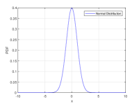
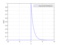
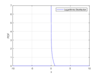
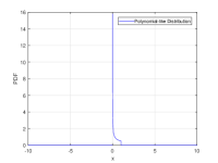
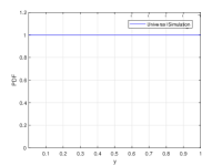
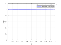
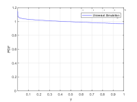
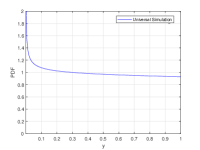
Figure 3: Universal simulations in Theorem 3.1 for the uniform distribution on $[0,1]$ by the mapping $x\mapsto\sum_{i=-\infty}^{\infty}\frac{1}{\Delta}(x-i\Delta)1\left\{x\in(i\Delta,(i+1)\Delta]\right\}$ with $\Delta=0.01$. The seed distributions $P_{X}$ are illustrated in top figures, which are respectively the standard Gaussian distribution $\mathcal{N}(0,1)$, exponential distribution $\mathrm{Exp}(1)$, logarithmic distribution $p_{X}(x)=-\log x,x\in(0,1]$, and polynomial-like distribution $p_{X}(x)=\left(1-r\right)x^{-r},x\in(0,1],r=0.5$. The generated distributions $P_{Y}$ are illustrated in bottom figures.

3.1.1 Relative Entropy and Rényi Divergence Measures

Next we extend Theorem 3.1 to the relative entropy and Rényi divergence measures. The relative entropy and Rényi divergence are two information measures that quantify the “distance” between probability measures.

Fix distributions $P_{X},Q_{X}\in\mathcal{P}(\mathbb{R},\mathcal{B}_{\mathbb{R}})$. The relative entropy and the Rényi divergence of order $\alpha\in(0,1)\cup(1,\infty)$ are respectively defined as

$$D(P_{X}\|Q_{X}) :=\int\left(\frac{dP_{X}}{dQ_{X}}\log\frac{dP_{X}}{dQ_{X}}\right)dQ_{X}$$

$$D_{\alpha}(P_{X}\|Q_{X}) :=\frac{1}{\alpha-1}\log\int\left(\frac{dP_{X}}{dQ_{X}}\right)^{\alpha}dQ_{X},$$

and the conditional versions are respectively defined as

$$D(P_{Y|X}\|Q_{Y|X}|P_{X}) :=D(P_{X}P_{Y|X}\|P_{X}Q_{Y|X})$$

$$D_{\alpha}(P_{Y|X}\|Q_{Y|X}|P_{X}) :=D_{\alpha}(P_{X}P_{Y|X}\|P_{X}Q_{Y|X}).$$

The Rényi divergence of order $\alpha\in\{0,1,\infty\}$ is defined by continuous extension. Throughout, $\log$ and $\exp$ are to the natural base $e$. It is known that $D_{1}(P_{X}\|Q_{X}):=\lim_{\alpha\to 1}D_{\alpha}(P_{X}\|Q_{X})=D(P_{X}\|Q_{X})$ so a special case of the Rényi divergence (resp. the conditional version) is the usual relative entropy (resp. the conditional version). The Rényi divergence of infinity order is defined as

$$D_{\infty}(P_{X}\|Q_{X}) :=\lim_{\alpha\to\infty}D_{\alpha}(P_{X}\|Q_{X})=\log\operatorname*{\mathrm{ess\,sup}}_{P_{X}}\frac{dP_{X}}{dQ_{X}}.$$

Definition 3.1.

A function $g:\mathcal{P}_{X}\to\mathbb{R}$ is called $\alpha$-Rényi-achievable for the universal $(\mathcal{P}_{X},Q_{Y})$-simulation, if there exists a sequence of simulators $\left\{f_{k}\right\}_{k=1}^{\infty}$ such that

$$\limsup_{k\to\infty}D_{\alpha}(P_{Y_{k}}\|Q_{Y})\leq g(P_{X})$$ (8)

for all $P_{X}\in\mathcal{P}_{X}$, where $P_{Y_{k}}:=P_{X}\circ f_{k}^{-1}$.

Definition 3.2.

The set of $\alpha$-Rényi-achievable functions for the universal $(\mathcal{P}_{X},Q_{Y})$-simulation is defined as

$$\mathcal{E}_{\mathrm{Renyi}}^{(\alpha)}(\mathcal{P}_{X},Q_{Y}):=\left\{g:\mathcal{P}_{X}\to\mathbb{R}\>:g\textrm{ is }\alpha\raisebox{0.75pt}{-}\textrm{R\'{e}nyi}\raisebox{0.75pt}{-}\textrm{achievable}\right\}.$$

For $\left(\mathcal{A},\mathcal{B}_{\mathcal{A}}\right)\subset\left(\mathbb{R},\mathcal{B}_{\mathbb{R}}\right)$, define

$$\mathcal{P}_{\mathrm{ac}}^{(\alpha)}\left(\mathcal{A},\mathcal{B}_{\mathcal{A}}\right):=\left\{P_{X}\in\mathcal{P}_{\mathrm{ac}}\left(\mathcal{A},\mathcal{B}_{\mathcal{A}}\right):\lim_{\Delta\to 0}\sup_{\left\{\mathcal{A}_{i}\right\}:\sup_{i}\left|\mathcal{A}_{i}\right|\leq\Delta}D_{\alpha}(P_{X|\left\{\mathcal{A}_{i}\right\}}\|P_{X})=0\right\},$$

where the supremum is taken over all partitions $\left\{\left\{\mathcal{A}_{i}\right\}:\mathcal{A}_{i}\textrm{ are intervals, and}\ \bigcup_{i}\mathcal{A}_{i}=\mathcal{A},\ \mathcal{A}_{i}\cap\mathcal{A}_{j}=\emptyset,\forall i\neq j\right\}$ of $\mathcal{A}$, $\left|\mathcal{A}_{i}\right|$ is the length of the interval $\mathcal{A}_{i}$, and $P_{X|\left\{\mathcal{A}_{i}\right\}}:=\frac{1\left\{x\in\mathcal{A}_{i}\right\}}{\left|\mathcal{A}_{i}\right|}P_{X}\left(\mathcal{A}_{i}\right)$. Based on the notations above, we have the following theorem.

Theorem 3.2.

Assume $\left(\mathcal{A},\mathcal{B}_{\mathcal{A}}\right)\subset\left(\mathbb{R},\mathcal{B}_{\mathbb{R}}\right)$,

$$\mathcal{P}_{X}=\begin{cases}\mathcal{P}_{\mathrm{ac}}&\alpha\in[0,1)\\ \mathcal{P}_{\mathrm{ac}}^{(\alpha)}\left(\mathcal{A},\mathcal{B}_{\mathcal{A}}\right)&\alpha\in[1,\infty]\end{cases},$$

and $Q_{Y}$ is arbitrary. Then for the universal $(\mathcal{P}_{X},Q_{Y})$-simulation problem, $\mathcal{E}_{\mathrm{Renyi}}^{(\alpha)}(\mathcal{P}_{X},Q_{Y})\asymp 0$.

Remark 3.1.

For $0<a\leq b<\infty$,

$$\mathcal{P}_{\mathrm{ac}}^{[a,b]}\left(\mathcal{A},\mathcal{B}_{\mathcal{A}}\right) :=\left\{P_{X}\in\mathcal{P}_{\mathrm{ac}}:a\leq p(x)\leq b\textrm{ a.e. in }\mathcal{A},\textrm{ and }P_{X}(\mathbb{R}\backslash\mathcal{A})=0\right\}$$

$$\subset\mathcal{P}_{\mathrm{ac}}^{(\alpha)}\left(\mathcal{A},\mathcal{B}_{\mathcal{A}}\right),\alpha\in[1,\infty]$$

Hence Theorem 3.2 still holds for $\mathcal{P}_{X}=\mathcal{P}_{\mathrm{ac}}^{[a,b]}\left(\mathcal{A},\mathcal{B}_{\mathcal{A}}\right)$ and $\alpha\in[1,\infty]$. Furthermore, Theorem 3.2 also holds if in (8) $D_{\alpha}(P_{Y_{k}}\|Q_{Y})$ is replaced with $D_{\alpha}(Q_{Y}\|P_{Y_{k}})$, $\alpha\in[0,\infty]$.

Proof.

It is easy to verify that (4) with the total variable distance replaced by the Rényi divergence still holds. This implies the cases $\alpha\in[1,\infty]$ in Theorem 3.2. The cases $\alpha\in[0,1)$ are implied by combining Theorem 3.1 with the following lemma which shows the “equivalence” between the Rényi divergence of order $\alpha\in(0,1)$ and the TV distance, in the sense that $D_{\alpha}(P_{X}\|Q_{X})\to 0$ if and only if $\left|P_{X}-Q_{X}\right|_{\mathrm{TV}}\to 0$. ∎

Lemma 3.1.

For $\alpha\in(0,1)$,

$$\frac{1}{\alpha-1}\log\left(1+\frac{1}{2}\left|P_{X}-Q_{X}\right|_{\mathrm{TV}}\right)\leq D_{\alpha}(P_{X}\|Q_{X})\leq\frac{1}{\alpha-1}\log\left(1-\frac{1}{2}\left|P_{X}-Q_{X}\right|_{\mathrm{TV}}\right).$$

Proof.

This lemma follows from the following two inequalities. Define $A:=\left\{x:P_{X}(x)\geq Q_{X}(x)\right\}$. Then

$$D_{\alpha}(P_{X}\|Q_{X}) =\frac{1}{\alpha-1}\log\left(\int_{A}\left(\frac{dP_{X}}{dQ_{X}}\right)^{\alpha}\mathrm{d}Q_{X}+\int_{\mathbb{R}\backslash A}\left(\frac{dQ_{X}}{dP_{X}}\right)^{1-\alpha}\mathrm{d}P_{X}\right)$$

$$\leq\frac{1}{\alpha-1}\log\left(\int_{A}dQ_{X}+\int_{\mathbb{R}\backslash A}dP_{X}\right)$$

$$=\frac{1}{\alpha-1}\log\left(1-\left(P_{X}\left(A\right)-Q_{X}\left(A\right)\right)\right)$$

$$=\frac{1}{\alpha-1}\log\left(1-\frac{1}{2}\left|P_{X}-Q_{X}\right|_{\mathrm{TV}}\right).$$

Similarly,

$$D_{\alpha}(P_{X}\|Q_{X}) \geq\frac{1}{\alpha-1}\log\left(1+\frac{1}{2}\left|P_{X}-Q_{X}\right|_{\mathrm{TV}}\right).$$

∎

3.2 Discontinuous seed distributions

Next we consider the case $\mathcal{P}_{X}\subseteq\mathcal{P}_{\mathrm{dc}}$. We first derive a discontinuous version of Theorem 3.1. Since in the previous subsection, Theorem 3.1 is proven only for absolutely continuous seed distributions, one may doubt the effectiveness of the proposed universal mapping in Fig. 2 when the seed distributions are discontinuous or even discrete. In the following, we prove that our proposed universal mapping still works well for discontinuous seed distributions, as long as the CDF of seed distribution is smooth enough.

Assume $\left\{\Delta_{n}\right\}$ is a sequence of non-increasing positive numbers. Assume $\left\{\mathcal{P}_{X_{n}}\right\}_{n=1}^{\infty}$ is a sequence of distribution sets such that for every sequence $\left\{P_{X_{n}}\right\}\in\left\{\mathcal{P}_{X_{n}}\right\}$, its CDFs $\left\{F_{X_{n}}\right\}$ satisfy

$$\lim_{n\to\infty}\sup_{x_{1}:F_{X_{n}}(x_{1}+\Delta_{n})>F_{X_{n}}(x_{1})}\sup_{x\in(x_{1},x_{1}+\Delta_{n}]}\left|\frac{F_{X_{n}}(x_{1}+x)-F_{X_{n}}(x_{1})}{F_{X_{n}}(x_{1}+\Delta_{n})-F_{X_{n}}(x_{1})}-\frac{x}{\Delta_{n}}\right|=0.$$ (9)

We obtain a discontinuous version of Theorem 3.1. The proof of Proposition 3.3 is provided in Appendix B.

Proposition 3.3.

Assume $\left\{\mathcal{P}_{X_{n}}\right\}$ is the sequence of distribution sets defined above. Then there exists a sequence of universal mappings $Y_{n}=f_{n}(X_{n})$ (which are dependent on $\left\{\Delta_{n}\right\}$) such that $\lim_{n\to\infty}\left|P_{Y_{n}}-Q_{Y}\right|_{\mathrm{KS}}=0,\forall\left\{P_{X_{n}}\right\}\in\left\{\mathcal{P}_{X_{n}}\right\}$. That is, $\lim_{n\to\infty}\mathcal{E}_{\mathrm{KS}}(\mathcal{P}_{X_{n}},Q_{Y})\asymp 0$.

The proposition above implies that if the CDF of seed random variable $X_{n}$ gets more and more smooth as $n\to\infty$ in the sense that it can be approximated by a linear function for every small interval $(x_{1},x_{1}+\Delta_{n}]$ as (9), then we can find a sequence of universal mappings that achieve vanishing KS-approximation error. Here is a simple example.

Example 3.2.

Assume $X$ is an absolutely continuous random variable with a bounded PDF. We define $X_{n}:=\frac{\left\lfloor nX\right\rfloor}{n}$ as a quantized version of $X$ with quantization step $\frac{1}{n}$, and $\Delta_{n}$ is set to $\frac{1}{\sqrt{n}}$, then $\left(\left\{X_{n}\right\},\left\{\Delta_{n}\right\}\right)$ satisfies (9).

The example above with $\frac{1}{n}=0.0001$, $\Delta=0.01$, and $P_{X}$ to be the standard Gaussian distribution or logarithmic distribution, is illustrated in Fig. 4.

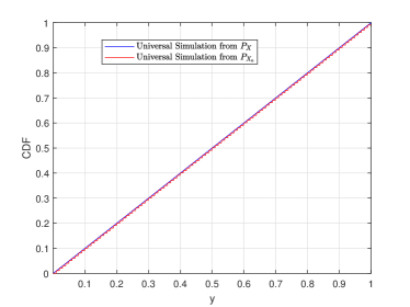
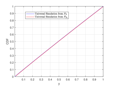
Figure 4: Universal simulations in Proposition 3.3 for the uniform distribution on $[0,1]$ by the mapping $x\mapsto\sum_{i=-\infty}^{\infty}\frac{1}{\Delta}(x-i\Delta)1\left\{x\in(i\Delta,(i+1)\Delta]\right\}$ with $\Delta=0.01$. The blue and red curves in the left figure correspond to the cases in which the seed distributions $P_{X}$ are respectively the standard Gaussian distribution $\mathcal{N}(0,1)$ and its quantized version. The blue and red curves in the right figure correspond to the cases in which the seed distributions $P_{X}$ are respectively the logarithmic distribution $p_{X}(x)=-\log x,x\in(0,1]$ and its quantized version. For both of these two cases, the quantized versions are generated by using the same quantization step $\frac{1}{n}=0.0001$.

If the seed is a sequence of i.i.d. discrete random vectors, then the approximation error decays exponentially fast. Given a Borel subset $\left(\mathcal{X},\mathcal{B}_{\mathcal{X}}\right)\subseteq\left(\mathbb{R},\mathcal{B}_{\mathbb{R}}\right)$ with $\mathcal{X}$ countable, $\mathcal{P}(\mathcal{X},\mathcal{B}_{\mathcal{X}})$ denotes the set of distributions on $\left(\mathcal{X},\mathcal{B}_{\mathcal{X}}\right)$.

Theorem 3.3.

Assume $\mathcal{P}_{X}=\mathcal{P}(\mathcal{X},\mathcal{B}_{\mathcal{X}})$ and $Q_{Y}$ is continuous. Then for the universal $(\mathcal{P}_{X}^{(n)},Q_{Y})$-simulation problem, $\mathcal{E}_{\mathrm{KS}}(\mathcal{P}_{X}^{(n)},Q_{Y})\mathrel{\dot{\asymp}}\left(\max_{x}P_{X}(x)\right)^{n}$.

Proof.

We first consider the case in which $\mathcal{X}$ is a finite set. We use a type-based mapping scheme to prove Theorem 3.3. Here we adopt the notation from [17]. We use $T_{x^{n}}\left(x\right):=\frac{1}{n}\sum_{i=1}^{n}1\left\{x_{i}=x\right\}$ to denote the type (empirical distribution) of a sequence $x^{n}$, and $T_{X}$ to denote a type of sequences in $\mathcal{X}^{n}$, where the indicator function $1\{A\}$ equals $1$ if the clause $A$ is true and $0$ otherwise. For a type $T_{X}$, the type class (set of sequences having the same type $T_{X}$) is denoted by $\mathcal{T}_{T_{X}}$. The set of types of sequences in $\mathcal{X}^{n}$ is denoted as $\mathcal{P}_{n}\left(\mathcal{X}\right):=\left\{T_{x^{n}}:x^{n}\in\mathcal{X}^{n}\right\}$. It has been shown that $\left|\mathcal{P}_{n}\left(\mathcal{X}\right)\right|\leq\left(n+1\right)^{\left|\mathcal{X}\right|}$ in [17].

For any i.i.d. $X^{n}$, all sequences in a type class have a equal probability. That is, under the condition $X^{n}\in\mathcal{T}_{T_{X}}$, it is uniformly distributed over the type class $\mathcal{T}_{T_{X}}$, regardless of $P_{X}$. Now we construct a mapping $f$ that maps the uniform random vector on $\mathcal{T}_{T_{X}}$ to a random variable such that $\sup_{y\in\mathbb{R}}\left|F_{Y}(y|T_{X})-G_{Y}(y)\right|$ is minimized. Here $F_{Y}(y|T_{X})$ denotes the CDF of the output random variable for the type $T_{X}$. Since the probability values of uniform random vectors are all equal to $\left|\mathcal{T}_{T_{X}}\right|^{-1}$, $\sup_{y\in\mathbb{R}}\left|F_{Y}(y|T_{X})-G_{Y}(y)\right|=\frac{1}{2}\left|\mathcal{T}_{T_{X}}\right|^{-1}$. Therefore, the output distribution induced by $f$ is

$$F_{Y}(y) =\sum_{T_{X}}\sum_{x^{n}\in\mathcal{T}_{T_{X}}}P_{X}^{n}(x^{n})1\{f(x^{n})\leq y\}$$ (10)

$$=\sum_{T_{X}}P_{X}^{n}(\mathcal{T}_{T_{X}})\sum_{x^{n}\in\mathcal{T}_{T_{X}}}\frac{P_{X}^{n}(x^{n})}{P_{X}^{n}(\mathcal{T}_{T_{X}})}1\{f(x^{n})\leq y\}$$

$$=\sum_{T_{X}}P_{X}^{n}(\mathcal{T}_{T_{X}})\sum_{x^{n}\in\mathcal{T}_{T_{X}}}\frac{1}{\left|\mathcal{T}_{T_{X}}\right|}1\{f(x^{n})\leq y\}$$

$$=\sum_{T_{X}}P_{X}^{n}(\mathcal{T}_{T_{X}})F_{Y}(y|T_{X})$$

$$\in\sum_{T_{X}}P_{X}^{n}(\mathcal{T}_{T_{X}})\left(G_{Y}(y)+\left[-\frac{1}{2}\left|\mathcal{T}_{T_{X}}\right|^{-1},\frac{1}{2}\left|\mathcal{T}_{T_{X}}\right|^{-1}\right]\right)$$

$$=G_{Y}(y)+\sum_{T_{X}}P_{X}^{n}(\mathcal{T}_{T_{X}})\left[-\frac{1}{2}\left|\mathcal{T}_{T_{X}}\right|^{-1},\frac{1}{2}\left|\mathcal{T}_{T_{X}}\right|^{-1}\right].$$

Using this equation we obtain

$$\left|F_{Y}(y)-G_{Y}(y)\right| \leq\frac{1}{2}\sum_{T_{X}}P_{X}^{n}(\mathcal{T}_{T_{X}})\left|\mathcal{T}_{T_{X}}\right|^{-1}$$

$$=\frac{1}{2}\sum_{T_{X}}e^{n\sum_{x}T_{X}(x)\log P_{X}(x)}$$

$$\leq\frac{1}{2}\left(n+1\right)^{\left|\mathcal{X}\right|}\max_{T_{X}}e^{n\sum_{x}T_{X}(x)\log P_{X}(x)}$$

$$\leq\frac{1}{2}e^{n\left(\log\max_{x}P_{X}(x)+\left|\mathcal{X}\right|\frac{\log\left(n+1\right)}{n}\right)}$$ (11)

$$\doteq e^{n\log\max_{x}P_{X}(x)}$$

$$=\left(\max_{x}P_{X}(x)\right)^{n}$$ (12)

We next consider the case in which $\mathcal{X}$ is countably infinite. For brevity, we assume $\mathcal{X}=\mathbb{Z}$. We partition $\mathbb{Z}$ into $2k+1$ intervals $\mathcal{U}_{-k}:=[-\infty:-k]$, $\mathcal{U}_{-\left(k-1\right)}:=\left\{-\left(k-1\right)\right\}$, …, $\mathcal{U}_{k-1}:=\left\{k-1\right\}$, $\mathcal{U}_{k}:=[k:\infty]$. Denote $Z_{k}=f_{1,k}(X)\in\mathcal{Z}:=[-k:k]$ as the index that $X\in\mathcal{U}_{Z_{k}}$. Hence $P_{Z_{k}}$ is defined on the finite set $\mathcal{Z}$. Now we use $Z_{k}$ to simulate $Y\sim Q_{Y}$. By the derivation above, we have that there exists a universal mapping $Y_{k}=f_{2,k}(Z_{k}):\mathcal{Z}\to\mathcal{Y}$ such that $\left|P_{Y_{k}}-Q_{Y}\right|_{\mathrm{KS}}\doteq\left(\max_{z}P_{Z_{k}}(z)\right)^{n}$. Furthermore, as $k\to\infty$, $\max_{z}P_{Z_{k}}(z)\to\max_{x}P_{X}(x)$. Therefore, the universal mappings $f_{2,k}\circ f_{1,k},k\in\mathbb{Z}$ satisfy $\limsup_{k\to\infty}\left|P_{Y_{k}}-Q_{Y}\right|_{\mathrm{KS}}\mathrel{\dot{\leq}}\left(\max_{x}P_{X}(x)\right)^{n}$.

The converse part follows from Theorem 2.3, since even non-universal simulation cannot make the approximation error decay faster than $\left(\max_{x}P_{X}(x)\right)^{n}$, hence universal simulation cannot as well. ∎

Now we consider a discontinuous $P_{X}$. We partition the real line into intervals $\mathcal{U}_{k}:=((k-1)\Delta,k\Delta],k\in\mathbb{Z}$ with $\Delta=\frac{1}{\sqrt{k}}$. Denote $Z_{k}=f_{1,k}(X)\in\mathbb{Z}$ as the index that $X\in\mathcal{U}_{Z_{k}}$. Hence $P_{Z_{k}}$ is defined on the set $\mathbb{Z}$. Now we use $Z_{k}$ to simulate $Y\sim Q_{Y}$. By Theorem 3.3, we have that there exists a universal mapping $Y_{k}=f_{2,k}(Z_{k}):\mathcal{Z}\to\mathcal{Y}$ such that $\left|P_{Y_{k}}-Q_{Y}\right|_{\mathrm{KS}}\doteq\left(\max_{z}P_{Z_{k}}(z)\right)^{n}$. Furthermore, as $k\to\infty$, we have $\max_{z}P_{Z_{k}}(z)\to\max_{x}P_{X}(x)$. Therefore, the universal mappings $f_{2,k}\circ f_{1,k},k\in\mathbb{Z}$ satisfy $\limsup_{k\to\infty}\left|P_{Y_{k}}-Q_{Y}\right|_{\mathrm{KS}}\mathrel{\dot{\leq}}\left(\max_{x}P_{X}(x)\right)^{n}$. Therefore, we have the following result.

Corollary 3.1.

Assume $\mathcal{P}_{X}=\mathcal{P}_{\mathrm{dc}}$ and $Q_{Y}$ is continuous. Then for the universal $(\mathcal{P}_{X}^{(n)},Q_{Y})$-simulation problem, $\mathcal{E}_{\mathrm{KS}}(\mathcal{P}_{X}^{(n)},Q_{Y})\mathrel{\dot{\asymp}}\left(\max_{x}P_{X}(x)\right)^{n}$.

3.3 Continuous but not absolutely continuous seed distributions

Next we consider continuous but not absolutely continuous $P_{X}$. For this case, we have $\max_{x}P_{X}(x)=0$. Hence the approximation error decays sup-exponentially fast. To provide a better bound, we assume $F_{X}$ is Hölder continuous with exponent $\alpha$, where $0<\alpha\leq 1$. That is, $L=\sup_{x_{1}\neq x_{2}}\frac{F_{X}(x_{2})-F_{X}(x_{1})}{\left(x_{2}-x_{1}\right)^{\alpha}}$ is finite. Consider the following mapping. We partition the real line into $2k+2$ intervals $U_{-k}:=(-\infty,-k\Delta]$, $U_{-\left(k-1\right)}:=(-k\Delta,-\left(k-1\right)\Delta]$, …, $U_{k}:=((k-1)\Delta,k\Delta]$, $U_{k+1}:=(k\Delta,\infty)$. Denote $Z=f_{1}(X)\in\mathcal{Z}:=[-k:k+1]$ as the index that $X\in U_{Z}$. Now we use $Z$ to simulate $Y\sim Q_{Y}$. By the derivation till (11), we have that there exists a universal mapping $Y=f_{2}(Z):\mathcal{Z}\to\mathcal{Y}$ such that $\left|P_{Y}-Q_{Y}\right|_{\mathrm{KS}}\leq\frac{1}{2}e^{n\left(\log\max_{z}P_{Z}(z)+\left(2k+2\right)\frac{\log\left(n+1\right)}{n}\right)}$. Set $\Delta=\frac{\log n}{n},k=\frac{n}{\sqrt{\log n}}$. Then $\Delta\to 0$ and $k\Delta=\sqrt{\log n}\to\infty$. Since $F_{X}$ is Hölder continuous with exponent $\alpha$, we have $\max_{z}P_{Z}(z)\leq\max_{x}\left\{F_{X}(x+\Delta)-F_{X}(x)\right\}\leq L\Delta^{\alpha}$. Hence the universal mapping $Y_{n}=f_{2}\circ f_{1}(X^{n})$ satisfies $\left|P_{Y_{n}}-Q_{Y}\right|_{\mathrm{KS}}=e^{-\alpha\Omega\left(n\log n\right)}$. Therefore, we have the following result.

Corollary 3.2.

Assume $\mathcal{P}_{X}=\mathcal{P}_{\mathrm{c}}\backslash\mathcal{P}_{\mathrm{ac}}$ and $Q_{Y}$ is arbitrary. Then for the universal $(\mathcal{P}_{X}^{(n)},Q_{Y})$-simulation problem, $\mathcal{E}_{\mathrm{KS}}(\mathcal{P}_{X}^{(n)},Q_{Y})\asymp e^{-\omega\left(n\right)}$. That is, there exists a sequence of simulators such that $\left|P_{Y^{(n)}}-Q_{Y}\right|_{\mathrm{KS}}$ decays sup-exponentially fast as $n\to\infty$ for any $P_{X}$. Moreover, if $\mathcal{P}_{X}=\left\{P_{X}:\>F_{X}\textrm{ is H\"{o}lder continuous with exponent }\alpha\right\}$ with $0<\alpha\leq 1$, then $\mathcal{E}_{\mathrm{KS}}(\mathcal{P}_{X}^{(n)},Q_{Y})\asymp e^{-\alpha\Omega\left(n\log n\right)}$.

4 Simulating a Random Variable from a Markov Process

In the preceding sections, we consider simulation of a random variable from a stationary memoryless process. Next we extend Theorem 3.3 to Markov processes of order $k\geq 1$.

Definition 4.1.

Given a Markov chain $\boldsymbol{X}=\left\{X_{n}:n\in\mathbb{N}\right\}$ of order $k\geq 1$ with finite state space $\mathcal{X}=\left\{1,2,...,|\mathcal{X}|\right\}$, initial state $x_{-k+1}^{0}:=(x_{-k+1},x_{-k+2},...,x_{0})$, and transition probability $P_{X_{k+1}|X^{k}}$, the min-entropy ($\infty$-order Rényi entropy) rate of $\boldsymbol{X}$ is defined as

$$H_{\text{$\infty$}}(\boldsymbol{X})=-\lim_{n\to\infty}\frac{1}{n}\max_{x^{n}}\log P(x^{n}).$$

Since the distribution of $X^{n}$ is determined by the initial state $x_{-k+1}^{0}$ and transition probability $P_{X_{k+1}|X^{k}}$, hence sometimes we also use $H_{\text{$\infty$}}(x_{-k+1}^{0},P_{X_{k+1}|X^{k}})$ to denote $H_{\text{$\infty$}}(\boldsymbol{X})$.

Given a state space $\mathcal{X}$ of any Markov chain $\left\{X_{n}:n\in\mathbb{N}\right\}$ of order $k=1$ with transition probability $P_{X_{k+1}|X^{k}}$, a loop is a sequence of distinct states of the chain $(i_{1},i_{2},...,i_{l})$ with $l\geq 1$ such that $P_{i_{s},i_{s+1}}>0$ for $s=1,2,...,l$ where $i_{l+1}=i_{1}$. (If $P_{i,i}>0$, then $(i)$ is a loop.) The set of all loops of length $l$ is denoted by $\mathcal{C}_{l}(P)$.

Let $P$ be the transition matrix of an ergodic Markov chain of order $k=1$ on a finite alphabet $\mathcal{X}$. The min-entropy rate of this Markov chain is given by [18]

$$H_{\text{$\infty$}}(\boldsymbol{X})=\min_{1\leq l\leq|\mathcal{X}|}\min\frac{1}{l}\sum_{s=1}^{l}\imath_{X_{2}|X_{1}}(i_{s+1}|i_{s})=\min_{1\leq l\leq|\mathcal{X}|}\min\frac{1}{l}\sum_{s=1}^{l}\log\frac{1}{p_{i_{s+1}i_{s}}},$$

where the inner minimum is taken over all loops $(i_{1},i_{2},...,i_{l})\in\mathcal{C}_{l}(P)$, and $\imath_{X_{2}|X_{1}}(j|i):=\log\frac{1}{P_{ij}}$.

4.1 Non-universal Simulation from a Markov Process

As a direct consequence of Proposition 2.1, we can obtain the approximation error for non-universal simulation from a Markov process.

Corollary 4.1.

Assume $\boldsymbol{X}=\left\{X_{n}:n\in\mathbb{N}\right\}$ is a Markov chain of order $k$ with finite state space $\mathcal{X}$, initial state $x_{-k+1}^{0}$, and transition probability $P_{X_{k+1}|X^{k}}$, and $Q_{Y}$ is a continuous distribution. Then for the non-universal $(P_{X^{n}},Q_{Y})$-simulation problem, $E_{\mathrm{KS}}(P_{X^{n}},Q_{Y})\doteq e^{-nH_{\text{$\infty$}}(x_{-k+1}^{0},P_{X_{k+1}|X^{k}})}$.

4.2 Universal Simulation from a Markov Process

Given a finite state space $\mathcal{X}$, a order $k\geq 1$, and a initial state $x_{-k+1}^{0}$, we denote the set of all possible distributions of Markov chains with these parameters as $\mathcal{P}_{X_{k+1}|X^{k}}^{(n)}:=\left\{\prod_{i=1}^{n}P_{X_{k+1}|X^{k}}(x_{i}|x_{i-1},...,x_{i-k}):P_{X_{k+1}|X^{k}}\in\mathcal{P}_{X_{k+1}|X^{k}}\right\}$, where $\mathcal{P}_{X_{k+1}|X^{k}}$ denotes the set of all possible transition probability $P_{X_{k+1}|X^{k}}$ (from $\mathcal{X}^{k}$ to $\mathcal{X}$).

We next consider universal simulation from a Markov process. We generalize Theorem 3.3 to this case. The proof of Theorem 4.1 is provided in Appendix C.

Theorem 4.1.

Assume $Q_{Y}$ is a continuous distribution. Then given a finite state space $\mathcal{X}$, an order $k$, and an initial state $x_{-k+1}^{0}$, for the universal $(\mathcal{P}_{X_{k+1}|X^{k}}^{(n)},Q_{Y})$-simulation problem, we have $\mathcal{E}_{\mathrm{KS}}(\mathcal{P}_{X_{k+1}|X^{k}}^{(n)},Q_{Y})\mathrel{\dot{\asymp}}e^{-nH_{\text{$\infty$}}(x_{-k+1}^{0},P_{X_{k+1}|X^{k}})}$.

5 Simulating a Random Element from another Random Element

5.1 Non-universal Simulation

Next we show that an arbitrary continuous random element (or general random variable) is sufficient to simulate another arbitrary random element. Here random elements is a generalization of random variable, which may be defined on any non-empty Borel set in a separable metric space.

Theorem 5.1.

Assume $P_{X}$ and $Q_{Y}$ are two distributions respectively defined on any non-empty Borel sets $(\mathcal{X},\mathcal{B}_{\mathcal{X}})$ and $(\mathcal{Y},\mathcal{B}_{\mathcal{Y}})$ in two Polish spaces (complete separable metric spaces). If $P_{X}$ is continuous, then there exists a measurable mapping $Y=f(X)$ such that $P_{Y}=Q_{Y}$. That is, $E_{\mathrm{TV}}(P_{X},Q_{Y})=0$.

Proof.

For any two Borel subsets of Polish spaces, they are Borel-isomorphic if and only if they have the same cardinality, which moreover is either finite, countable, or $\mathfrak{c}$ (the cardinal of the continuum, that is, of $[0,1]$) [14]. Hence for any measurable space $(\mathcal{X},\mathcal{B}_{\mathcal{X}})$, we can always find a Borel subset $(\mathcal{W},\mathcal{B}_{\mathcal{W}})$ of $([0,1],\mathcal{B}_{[0,1]})$ such that $(\mathcal{X},\mathcal{B}_{\mathcal{X}})$ and $(\mathcal{W},\mathcal{B}_{\mathcal{W}})$ are Borel-isomorphic. Suppose $\varphi$ is a Borel isomorphism from $(\mathcal{X},\mathcal{B}_{\mathcal{X}})$ to $(\mathcal{W},\mathcal{B}_{\mathcal{W}})$. Denote $P_{W}:=P_{X}\circ\varphi^{-1}$. Since $P_{X}$ is continuous (or atomless), $P_{W}$ must be continuous as well. This is because if $P_{X}(\varphi^{-1}(w))=P_{W}(w)>0$ for some $w\in[0,1]$, then it contradicts with the continuity of $P_{X}$. Hence $P_{W}$ is continuous. (Furthermore, the existence of the Borel isomorphism $\varphi$ can be shown by [19, Theorem 9.2.2] as well.)

Similarly, for any measurable space $(\mathcal{Y},\mathcal{B}_{\mathcal{Y}})$, we can always find a Borel subset $(\mathcal{Z},\mathcal{B}_{\mathcal{Z}})$ of $(\mathbb{R},\mathcal{B}_{\mathbb{R}})$ such that $(\mathcal{Y},\mathcal{B}_{\mathcal{Y}})$ and $(\mathcal{Z},\mathcal{B}_{\mathcal{Z}})$ are Borel-isomorphic. Suppose $\phi$ is a Borel isomorphism from $(\mathcal{Y},\mathcal{B}_{\mathcal{Y}})$ to $(\mathcal{Z},\mathcal{B}_{\mathcal{Z}})$. Denote $Q_{Z}$ as the distribution of $\tilde{Z}:=\phi(\tilde{Y})$ with $\tilde{Y}\sim Q_{Y}$.

By Proposition 2.1, we know that there exists a measurable mapping $\eta$ such that $Z:=\eta(W)\sim Q_{Z}$ with $W\sim P_{W}$. Now consider the mapping $Y=\phi^{-1}\circ\eta\circ\varphi(X)$. Obviously, $Y=\phi^{-1}(Z)\sim Q_{Y}$. ∎

Note that random vectors defined on $(\mathbb{R}^{n},\mathcal{B}_{\mathbb{R}^{n}}),n\in\mathbb{Z}^{+}$ are special cases of such random elements. Hence we have the following corollary.

Corollary 5.1.

For a continuous $P_{X}$ defined on $(\mathbb{R},\mathcal{B}_{\mathbb{R}})$ and an arbitrary $Q_{Y^{n}}$ defined on $(\mathbb{R}^{n},\mathcal{B}_{\mathbb{R}^{n}}),n\in\mathbb{Z}^{+}$, there exists a measurable mapping $Y^{n}=f(X):\mathbb{R}\to\mathbb{R}^{n}$ such that $P_{Y^{n}}=Q_{Y^{n}}$.

5.2 Universal Simulation

Now we generalize Theorem 3.1 to simulating random elements.

Theorem 5.2.

Assume $R_{X}$ and $Q_{Y}$ are two distributions respectively defined on any non-empty Borel sets $(\mathcal{X},\mathcal{B}_{\mathcal{X}})$ and $(\mathcal{Y},\mathcal{B}_{\mathcal{Y}})$ in two Polish spaces, and moreover, $R_{X}$ is continuous. $\mathcal{P}_{X}(R_{X})$ denotes the set of all absolutely continuous distributions (defined on $(\mathcal{X},\mathcal{B}_{\mathcal{X}})$) respect to $R_{X}$. Then for the universal $(\mathcal{P}_{X}(R_{X}),Q_{Y})$-simulation problem, $\mathcal{E}_{\mathrm{TV}}(\mathcal{P}_{X}(R_{X}),Q_{Y})\asymp 0$.

Proof.

Since $R_{X}$ is continuous, as shown in the proof of Theorem 5.1, there exists a Borel isomorphism $\varphi$ from $(\mathcal{X},\mathcal{B}_{\mathcal{X}})$ to a Borel subset $(\mathcal{W},\mathcal{B}_{\mathcal{W}})$ of $([0,1],\mathcal{B}_{[0,1]})$ such that the output distribution $R_{X}\circ\varphi^{-1}$ is continuous. Denote $R_{Z}$ as the uniform distribution (which is also the Lebesgue measure) on $([0,1],\mathcal{B}_{[0,1]})$. Then by Proposition 2.1, we know that there exists a measurable mapping $\eta:(\mathcal{W},\mathcal{B}_{\mathcal{W}})\to([0,1],\mathcal{B}_{[0,1]})$ such that

$$R_{X}\circ\varphi^{-1}\circ\eta^{-1}=R_{Z}.$$ (13)

Hence a random element $\tilde{X}\sim R_{X}$ is mapped to a uniform random variable $\tilde{Z}\sim R_{Z}$ through the mapping $\tilde{Z}=\eta\circ\varphi(\tilde{X})$. We define $P_{Z}:=P_{X}\circ\varphi^{-1}\circ\eta^{-1}$, which denotes the distribution of $Z=\eta\circ\varphi(X)$ where $X\sim P_{X}$. Since $P_{X}$ is absolutely continuous respect to $R_{X}$, we have that $P_{Z}$ is absolutely continuous respect to $R_{Z}$ (or the Lebesgue measure). This is because on one hand, by (13), we have $R_{X}(\varphi^{-1}\circ\eta^{-1}(A))=0$ for any $A$ such that $R_{Z}(A)=0$; on the other hand, $P_{X}$ is absolutely continuous respect to $R_{X}$, hence $P_{X}(\varphi^{-1}\circ\eta^{-1}(A))=0$, i.e., $P_{Z}(A)=0$.

Since $P_{Z}$ is absolutely continuous, by Theorem 3.1, we know that there exists a sequence of universal mappings $\tau_{k}:([0,1],\mathcal{B}_{[0,1]})\to([0,1],\mathcal{B}_{[0,1]})$ (independent of $P_{Z}$) such that the resulting approximation error

$$\lim_{k\to\infty}\left|P_{Z}\circ\tau_{k}^{-1}-R_{Z}\right|_{\mathrm{TV}}=0.$$

Observe that $P_{Z}=P_{X}\circ\varphi^{-1}\circ\eta^{-1}$ and $\eta,\varphi$ (only depend on $R_{X}$) are independent of $P_{X}$. Hence the universal mappings $\tau_{k}\circ\eta\circ\varphi$ satisfy

$$\lim_{k\to\infty}\left|P_{X}\circ\varphi^{-1}\circ\eta^{-1}\circ\tau_{k}^{-1}-R_{Z}\right|_{\mathrm{TV}}=0.$$ (14)

Since $R_{Z}$ is continuous, by Theorem 5.1, we know that then there exists a measurable mapping $\kappa:([0,1],\mathcal{B}_{[0,1]})\to(\mathcal{Y},\mathcal{B}_{\mathcal{Y}})$ such that $R_{Z}\circ\kappa^{-1}=Q_{Y}$.

Now we consider the universal mappings $Y=\kappa\circ\tau_{k}\circ\eta\circ\varphi(X)$. We have

$$\left|P_{X}\circ\varphi^{-1}\circ\eta^{-1}\circ\tau_{k}^{-1}\circ\kappa^{-1}-Q_{Y}\right|_{\mathrm{TV}} =\sup_{A\in\mathcal{B}_{\mathcal{Y}}}\left|P_{X}\circ\varphi^{-1}\circ\eta^{-1}\circ\tau_{k}^{-1}\circ\kappa^{-1}(A)-Q_{Y}(A)\right|$$

$$=\sup_{A\in\mathcal{B}_{\mathcal{Y}}}\left|P_{X}\circ\varphi^{-1}\circ\eta^{-1}\circ\tau_{k}^{-1}(\kappa^{-1}(A))-R_{Z}(\kappa^{-1}(A))\right|$$

$$\leq\sup_{B\in\mathcal{B}_{[0,1]}}\left|P_{X}\circ\varphi^{-1}\circ\eta^{-1}\circ\tau_{k}^{-1}(B)-R_{Z}(B)\right|$$

$$=\left|P_{X}\circ\varphi^{-1}\circ\eta^{-1}\circ\tau_{k}^{-1}-R_{Z}\right|_{\mathrm{TV}}.$$

Combining this with (14) yields

$$\lim_{k\to\infty}\left|P_{X}\circ\varphi^{-1}\circ\eta^{-1}\circ\tau_{k}^{-1}\circ\kappa^{-1}-Q_{Y}\right|_{\mathrm{TV}}=0.$$

∎

Note that a random vector defined on $(\mathbb{R}^{n},\mathcal{B}_{\mathbb{R}^{n}}),n\in\mathbb{Z}^{+}$ is a special case of such a random element. Furthermore, for any absolutely continuous (respect to the Lebesgue measure) $P_{X^{n}}$ defined on $(\mathbb{R}^{n},\mathcal{B}_{\mathbb{R}^{n}}),n\in\mathbb{Z}^{+}$, it must be absolutely continuous respect to the $n$-dimensional standard Gaussian distribution (since its PDF is positive for every point in $\mathbb{R}^{n}$). Hence we have the following corollary.

Corollary 5.2.

For the set $\mathcal{P}_{\mathrm{ac}}$ of absolutely continuous distributions on $(\mathbb{R},\mathcal{B}_{\mathbb{R}})$ and an arbitrary $Q_{Y^{n}}$ on $(\mathbb{R}^{n},\mathcal{B}_{\mathbb{R}^{n}}),n\in\mathbb{Z}^{+}$, the approximation errors for the universal $(\mathcal{P}_{\mathrm{ac}},Q_{Y^{n}})$-simulation problem satisfies $\mathcal{E}_{\theta}(\mathcal{P}_{\mathrm{ac}},Q_{Y^{n}})\asymp 0$ for $\theta\in\left\{\mathrm{KS},\mathrm{TV}\right\}$.

6 Concluding Remarks

In this paper, motivated by the CLT and other universal simulation problems in the literature, we consider both universal and non-universal simulations of random variables with an arbitrary target distribution $Q_{Y}$ by general mappings. We investigate the fastest convergence rate of the approximation error for such a problem. One of our interesting results is that under universal simulation, an absolutely continuous random element (or a general random variable, including random vectors) respect to some continuous distribution is sufficient to simulate another random element arbitrarily well. This requirement is a little stronger than that for non-universal simulation, since under non-universal simulation, a continuous random element is sufficient to exactly simulate another random element. Another interesting result is that when we use a stationary memoryless process or a Markov process to simulate a random variable by a universal mapping, the approximation error decays at least exponentially fast with rate $H_{\infty}(P_{X}):=-\log\max_{x}P_{X}(x)$ as the dimension $n$ of $X^{n}$ goes to infinity. Furthermore, as a byproduct, we also obtain a property on uncorrelation between a squeezed periodic function and any other integrable function. We think this topic is of independent interest, and expect it to be further applied in other problems in the future.

As for application aspects of our results, although practical digital computers have finite precision for processing or storing datum, as indicated by Proposition 3.3, our proposed universal mapping in Fig. 2 still works well on such digital computers, as long as they have sufficiently high precision; see the illustration in Fig. 4.

Appendix A Proof of Proposition 2.3

Sort the sequences in $\mathcal{X}{}^{n}$ as $x_{1}^{n},x_{2}^{n},...,x_{|\mathcal{X}|^{n}}^{n}$ such that $P_{X}^{n}(x_{1}^{n})\geq P_{X}^{n}(x_{2}^{n})\geq...\geq P_{X}^{n}(x_{|\mathcal{X}|^{n}}^{n})$. Map $x_{1}^{n}$ to $y_{1}:=\arg\max_{y\in\mathcal{Y}}Q_{Y}(y)$; map $x_{2}^{n}$ to $y_{2}:=\arg\max_{y\in\mathcal{Y}}\left\{Q_{Y}(y)-P_{X}^{n}(x_{1}^{n})1\left\{y=y_{1}\right\}\right\}$; …; map $x_{|\mathcal{X}|^{n}-|\mathcal{Y}|-2}^{n}$ to $y_{|\mathcal{X}|^{n}-|\mathcal{Y}|-1}:=\arg\max_{y\in\mathcal{Y}}\bigl{\{}Q_{Y}(y)-\sum_{i=1}^{|\mathcal{X}|^{n}-|\mathcal{Y}|-1}P_{X}^{n}(x_{i}^{n})1\left\{y=y_{i}\right\}\bigr{\}}$. Map the remaining $|\mathcal{Y}|+1$ sequences $x_{j}^{n},|\mathcal{X}|^{n}-|\mathcal{Y}|\leq j\leq|\mathcal{X}|^{n}$ to sequences in $\mathcal{Y}$ in a similar way as in the proof of Proposition 2.2, such that $\sup_{y\in\mathbb{R}}\left|\sum_{y^{\prime}\leq y}\sum_{i=1}^{j}P_{X}^{n}(x_{i}^{n})1\left\{y^{\prime}=y_{i}\right\}-G_{Y}(y)\right|$ is minimized for $|\mathcal{X}|^{n}-|\mathcal{Y}|\leq j\leq|\mathcal{X}|^{n}$.

For this mapping, observe that for any $1\leq j\leq|\mathcal{X}|^{n}$,

$$\max_{y\in\mathcal{Y}}\left\{Q_{Y}(y)-\sum_{i=1}^{j}P_{X}^{n}(x_{i}^{n})1\left\{y=y_{i}\right\}\right\} \geq\frac{\sum_{y\in\mathcal{Y}}\left\{Q_{Y}(y)-\sum_{i=1}^{j}P_{X}^{n}(x_{i}^{n})1\left\{y=y_{i}\right\}\right\}}{|\mathcal{Y}|}$$

$$=\frac{1-\sum_{i=1}^{j}P_{X}^{n}(x_{i}^{n})}{|\mathcal{Y}|}$$

$$=\frac{\sum_{i=j+1}^{|\mathcal{X}|^{n}}P_{X}^{n}(x_{i}^{n})}{|\mathcal{Y}|}.$$

This implies that if $P_{X}^{n}(x_{j+1}^{n})\leq\frac{\sum_{i=j+1}^{|\mathcal{X}|^{n}}P_{X}^{n}(x_{i}^{n})}{|\mathcal{Y}|}$, then $\sum_{i=1}^{j+1}P_{X}^{n}(x_{i}^{n})1\left\{y_{j+1}=y_{i}\right\}\leq Q_{Y}(y_{j+1})$. Therefore, the following claim holds.

Claim A.1.

If $P_{X}^{n}(x_{j+1}^{n})\leq\frac{\sum_{i=j+1}^{|\mathcal{X}|^{n}}P_{X}^{n}(x_{i}^{n})}{|\mathcal{Y}|}$ holds for $1\leq j\leq m$ (for some integer $m$), then $\sum_{i=1}^{m+1}P_{X}^{n}(x_{i}^{n})1\left\{y=y_{i}\right\}\leq Q_{Y}(y)$ for all $y\in\mathcal{Y}$.

Next we prove the following claim.

Claim A.2.

$P_{X}^{n}(x_{j+1}^{n})\leq\frac{\sum_{i=j+1}^{|\mathcal{X}|^{n}}P_{X}^{n}(x_{i}^{n})}{|\mathcal{Y}|}$ holds for $1\leq j\leq|\mathcal{X}|^{n}-|\mathcal{Y}|-2$ and for $n\geq|\mathcal{Y}|\max_{1\leq i\leq|\mathcal{X}|-1}\frac{P_{X}(x_{i})}{P_{X}(x_{i+1})}$.

We split the proof into two cases.

• Case 1 ($1\leq j\leq|\mathcal{X}|^{n}-n-2$): For $1\leq j\leq|\mathcal{X}|^{n}-n-2$, denote $k$ as the smallest integer such that $k\geq j+2$ and $T_{x_{k}^{n}}\neq T_{x_{j+1}^{n}}$. Then we have

  $$P_{X}^{n}(x_{j+1}^{n})\leq P_{X}^{n}(x_{k}^{n})\max_{1\leq i\leq|\mathcal{X}|-1}\frac{P_{X}(x_{i})}{P_{X}(x_{i+1})}.$$ (15)

  This is because if $x_{k}^{n}$ and $x_{j+1}^{n}$ are different in only one component, say the $i$th components $x_{k,i}$ and $x_{j+1,i}$, then by the generation process of $x_{1}^{n},x_{2}^{n},...,x_{|\mathcal{X}|^{n}}^{n}$, we have $\frac{P_{X}(x_{k,i})}{P_{X}(x_{j+1,i})}\geq\min_{1\leq i\leq|\mathcal{X}|-1}\frac{P_{X}(x_{i+1})}{P_{X}(x_{i})}$. Hence

  $$P_{X}^{n}(x_{j+1}^{n})=P_{X}^{n}(x_{k}^{n})\frac{P_{X}(x_{j+1,i})}{P_{X}(x_{k,i})}\leq P_{X}^{n}(x_{k}^{n})\max_{1\leq i\leq|\mathcal{X}|-1}\frac{P_{X}(x_{i})}{P_{X}(x_{i+1})}.$$

  If $x_{k}^{n}$ and $x_{j+1}^{n}$ are different in more than one components, then by the generation process of $x_{1}^{n},x_{2}^{n},...,x_{|\mathcal{X}|^{n}}^{n}$, we have $P_{X}^{n}(x_{j+1}^{n})\geq P_{X}^{n}(x_{k}^{n})\geq P_{X}^{n}(\tilde{x}_{k}^{n})$ for any sequence $\tilde{x}_{k}^{n}$ such that $\tilde{x}_{k}^{n}$ are different from $x_{j+1}^{n}$ in only one component. Hence by the same argument above, we obtain

  $$P_{X}^{n}(x_{j+1}^{n})\leq P_{X}^{n}(\tilde{x}_{k}^{n})\max_{1\leq i\leq|\mathcal{X}|-1}\frac{P_{X}(x_{i})}{P_{X}(x_{i+1})}\leq P_{X}^{n}(x_{k}^{n})\max_{1\leq i\leq|\mathcal{X}|-1}\frac{P_{X}(x_{i})}{P_{X}(x_{i+1})}.$$

  Therefore, (15) holds. Next, we prove (15) implies Claim A.2.

  $$\frac{P_{X}^{n}(x_{j+1}^{n})}{\sum_{i=j+1}^{|\mathcal{X}|^{n}}P_{X}^{n}(x_{i}^{n})} \leq\frac{P_{X}^{n}(x_{j+1}^{n})}{\sum_{i=k}^{|\mathcal{X}|^{n}}P_{X}^{n}(x_{i}^{n})}$$

  $$\leq\frac{P_{X}^{n}(x_{k}^{n})\max_{1\leq i\leq|\mathcal{X}|-1}\frac{P_{X}(x_{i})}{P_{X}(x_{i+1})}}{\sum_{i=k}^{|\mathcal{X}|^{n}}P_{X}^{n}(x_{i}^{n})}$$

  According to the definition of $x_{k}^{n}$, we have $\mathcal{T}_{T_{x_{k}^{n}}}\subseteq\left\{x_{k}^{n},x_{k+1}^{n},...,x_{|\mathcal{X}|^{n}}^{n}\right\}$. Furthermore, each type class has at least $n$ elements, hence $\left|\mathcal{T}_{T_{x_{k}^{n}}}\right|\geq n$. Therefore,

  $$\frac{P_{X}^{n}(x_{k}^{n})\max_{1\leq i\leq|\mathcal{X}|-1}\frac{P_{X}(x_{i})}{P_{X}(x_{i+1})}}{\sum_{i=k}^{|\mathcal{X}|^{n}}P_{X}^{n}(x_{i}^{n})} \leq\frac{P_{X}^{n}(x_{k}^{n})\max_{1\leq i\leq|\mathcal{X}|-1}\frac{P_{X}(x_{i})}{P_{X}(x_{i+1})}}{nP_{X}^{n}(x_{k}^{n})}$$

  $$=\frac{\max_{1\leq i\leq|\mathcal{X}|-1}\frac{P_{X}(x_{i})}{P_{X}(x_{i+1})}}{n}$$ (16)

  For $n\geq|\mathcal{Y}|\max_{1\leq i\leq|\mathcal{X}|-1}\frac{P_{X}(x_{i})}{P_{X}(x_{i+1})}$, we have (16) $\leq\frac{1}{|\mathcal{Y}|}$. Therefore, $P_{X}^{n}(x_{j+1}^{n})\leq\frac{\sum_{i=j+1}^{|\mathcal{X}|^{n}}P_{X}^{n}(x_{i}^{n})}{|\mathcal{Y}|}$.

• Case 2 ($|\mathcal{X}|^{n}-n-1\leq j\leq|\mathcal{X}|^{n}-|\mathcal{Y}|-2$): For $|\mathcal{X}|^{n}-n-1\leq j\leq|\mathcal{X}|^{n}-|\mathcal{Y}|-2$, we know $x_{j+1}^{n},...,x_{|\mathcal{X}|^{n}-1}^{n}$ belong to a same type class, $P(x_{j+1}^{n})=...=P(x_{|\mathcal{X}|^{n}-1}^{n})=\left(P_{X}(x_{|\mathcal{X}|})\right)^{n-1}P_{X}(x_{|\mathcal{X}|-1})$, and $P(x_{|\mathcal{X}|^{n}}^{n})=\left(P_{X}(x_{|\mathcal{X}|})\right)^{n}$. Hence we have $\frac{P_{X}^{n}(x_{j+1}^{n})}{\sum_{i=j+1}^{|\mathcal{X}|^{n}}P_{X}^{n}(x_{i}^{n})}\leq\frac{P_{X}^{n}(x_{j+1}^{n})}{|\mathcal{Y}|P_{X}^{n}(x_{j+1}^{n})}=\frac{1}{|\mathcal{Y}|}$.

Combining the two cases above, we have Claim A.2. By Claim A.1, we further have $\sum_{i=1}^{m+1}P_{X}^{n}(x_{i}^{n})1\left\{y=y_{i}\right\}\leq Q_{Y}(y)$ for all $y\in\mathcal{Y}$ with $m=|\mathcal{X}|^{n}-|\mathcal{Y}|-2$.

Since the remaining $|\mathcal{Y}|+1$ sequences are mapped to sequences in $\mathcal{Y}$ in a similar way as in the proof of Proposition 2.2, similar to Proposition 2.2, here we can show that the output measure $P_{Y}$ induced by the mapping satisfies $\left|P_{Y}-Q_{Y}\right|_{\mathrm{KS}}\leq\frac{1}{2}P_{X}(x_{|\mathcal{X}|-1})\left(P_{X}(x_{|\mathcal{X}|})\right)^{n-1}$.

Appendix B Proof of Proposition 3.3

Universal Mapping: For $X_{n}$, partition the real line into intervals with the same length $\Delta_{n}$, i.e., $\bigcup_{i=-\infty}^{\infty}(i\Delta_{n},(i+1)\Delta_{n}]$. We first simulate a uniform distribution on $[a,b]$ by mapping each interval $(i\Delta_{n},(i+1)\Delta_{n}]$ into $[a,b]$ using the linear function $x\mapsto a+\frac{b-a}{\Delta_{n}}(x-i\Delta_{n})$. That is, the function used here is

$$f_{1}(x):=\sum_{i=-\infty}^{\infty}\left(a+\frac{b-a}{\Delta_{n}}(x-i\Delta_{n})\right)1\left\{x\in(i\Delta_{n},(i+1)\Delta_{n}]\right\}.$$

We then transform the output distribution to the target distribution $Q_{Y}$, by using function $x\mapsto G_{Y}^{-1}\left(\frac{x-a}{b-a}\right)$, where $G_{Y}^{-1}\left(t\right):=\min\left\{y:G_{Y}(y)\geq t\right\}$. Therefore, each $x\in(i\Delta_{n},(i+1)\Delta_{n}]$ is mapped to $G_{Y}^{-1}\left(\frac{1}{\Delta}(x-i\Delta)\right)$. Hence the final mapping is

$$f(x):=\sum_{i=-\infty}^{\infty}G_{Y}^{-1}\left(\frac{1}{\Delta_{n}}(x-i\Delta_{n})\right)1\left\{x\in(i\Delta_{n},(i+1)\Delta_{n}]\right\}.$$

For such a universal simulator, we have

$$\left|P_{Y_{n}}-Q_{Y}\right|_{\mathrm{KS}} \leq\left|P_{f_{1}(X_{n})}-\mathrm{Unif}([a,b])\right|_{\mathrm{KS}}$$ (17)

$$=\sup_{z\in[a,b]}\left|\sum_{i=-\infty}^{\infty}\left[F_{X_{n}}\left(i\Delta_{n}+\Delta_{n}\frac{z-a}{b-a}\right)-F_{X_{n}}(i\Delta_{n})\right]-\frac{z-a}{b-a}\right|$$

$$=\sup_{x\in[0,\Delta_{n}]}\left|\sum_{i=-\infty}^{\infty}\left[F_{X_{n}}(i\Delta_{n}+x)-F_{X_{n}}(i\Delta_{n})\right]-\frac{x}{\Delta_{n}}\right|$$

$$=\sup_{x\in[0,\Delta_{n}]}\left|\sum_{i=-\infty}^{\infty}\left[F_{X_{n}}((i+1)\Delta_{n})-F_{X_{n}}(i\Delta_{n})\right]\left(\frac{F_{X_{n}}(i\Delta_{n}+x)-F_{X_{n}}(i\Delta_{n})}{F_{X_{n}}((i+1)\Delta_{n})-F_{X_{n}}(i\Delta_{n})}-\frac{x}{\Delta_{n}}\right)\right|$$

$$\leq\sum_{i=-\infty}^{\infty}\left[F_{X_{n}}((i+1)\Delta_{n})-F_{X_{n}}(i\Delta_{n})\right]\sup_{x\in[0,\Delta_{n}]}\left|\frac{F_{X_{n}}(i\Delta_{n}+x)-F_{X_{n}}(i\Delta_{n})}{F_{X_{n}}((i+1)\Delta_{n})-F_{X_{n}}(i\Delta_{n})}-\frac{x}{\Delta_{n}}\right|$$

$$\leq\sup_{x_{1}:F_{X_{n}}(x_{1}+\Delta_{n})>F_{X_{n}}(x_{1})}\sup_{x\in(x_{1},x_{1}+\Delta_{n}]}\left|\frac{F_{X_{n}}(x_{1}+x)-F_{X_{n}}(x_{1})}{F_{X_{n}}(x_{1}+\Delta_{n})-F_{X_{n}}(x_{1})}-\frac{x}{\Delta_{n}}\right|$$

$$\to 0,\textrm{ as }n\to\infty,$$

where (17) follows from Lemma 1.1.

Appendix C Proof of Theorem 4.1

We still use a type-based mapping scheme (similar to that used in the proof of Theorem 3.3) to prove Theorem 4.1.

Here we adopt the notation from [20]. Assume the Markov process $\boldsymbol{X}$ starts from the fixed initial state $(x_{-k+1},x_{-k+2},...,x_{0})$. The $k$-th order Markov type $T_{x^{n}}$ of a sequence $x^{n}\in\mathcal{X}^{n}$ is defined as the number of occurrences in $x^{n}$ of each string $\boldsymbol{s}\in\mathcal{X}^{k+1}$, denoted $n_{x^{n}}(\boldsymbol{s})$, namely

$$n_{x^{n}}(\boldsymbol{s})=\left|\left\{i:1\leq i\leq n,(x_{i-k},...,x_{i-1},x_{i})=\boldsymbol{s}\right\}\right|$$

where $\left|\cdot\right|$ denotes cardinality. We use $T_{k}$ to denote a $k$-th order Markov type of sequences in $\mathcal{X}^{n}$. For a type $T_{k}$, the $k$-th order Markov type class $\mathcal{T}_{T_{k}}$ is the set of all sequences $x^{n}\in\mathcal{X}^{n}$ that have the same type $T_{k}$. Obviously, all sequences in a type class have a equal probability, i.e, $P(x^{n})=P(\tilde{x}^{n})$ for all $x^{n},\tilde{x}^{n}\in\mathcal{T}_{T_{k}}$. That is, under the condition $X^{n}\in\mathcal{T}_{T_{k}}$, it is uniformly distributed over the type class $\mathcal{T}_{T_{k}}$, regardless of the distribution of the Markov process. Furthermore, the set of $k$-th order Markov types of sequences in $\mathcal{X}^{n}$ is denoted as $\mathcal{P}_{k,n}\left(\mathcal{X}\right):=\left\{T_{x^{n}}:x^{n}\in\mathcal{X}^{n}\right\}$. It has been shown that $\left|\mathcal{P}_{k,n}\left(\mathcal{X}\right)\right|\leq\left(n+1\right)^{\left|\mathcal{X}\right|^{k+1}}$ in [20].

Now we construct a mapping $f$ that maps the uniform random vector on $\mathcal{T}_{T_{k}}$ to a random variable such that $\sup_{y\in\mathbb{R}}\left|F_{Y}(y|T_{k})-G_{Y}(y)\right|$ is minimized. Here $F_{Y}(y|T_{k})$ denotes the CDF of the output random variable for the uniform random vector on $\mathcal{T}_{T_{k}}$. Since the probability values of uniform random vectors are all equal to $\left|\mathcal{T}_{T_{k}}\right|^{-1}$, $\sup_{y\in\mathbb{R}}\left|F_{Y}(y|T_{k})-G_{Y}(y)\right|=\frac{1}{2}\left|\mathcal{T}_{T_{k}}\right|^{-1}$. Following the same steps as (10)-(12), we obtain

$$\left|F_{Y}(y)-G_{Y}(y)\right| \mathrel{\dot{\leq}}\max_{x^{n}}P(x^{n}).$$

The converse part follows from Theorem 2.3, since even non-universal simulation cannot make the approximation error decay faster than $\max_{x^{n}}P(x^{n})$, hence universal simulation cannot as well.

Appendix D Properties on Squeezing Periodic Functions

For a function $g:[a,b]\to\mathbb{R}$ and a number $\Delta>0$, we define a periodic function $g_{\Delta}$ induced by $g$ as

$$g_{\Delta}(x):=\sum_{i=-\infty}^{\infty}g\left(a+\frac{b-a}{\Delta}(x-i\Delta)\right)1\left\{x\in(i\Delta,(i+1)\Delta]\right\}.$$

Now we squeeze this periodic function in the $x$-axis direction by letting $\Delta\to 0$. It is easy to see that the limit $\lim_{\Delta\to 0}g\left(a+\frac{b-a}{\Delta}(x-i\Delta)\right)$ of function $g$ does not exist. However, the integral $\lim_{\Delta\to 0}\int f(x)g_{\Delta}(x)dx$ for any integrable function $f$ exists. Moreover, this limit is equal to the product of the integral of $f(x)$ and the normalized integral of $g_{\Delta}(x)$ (or $g\left(x\right)$). That is, $f(x)$ and $g_{\Delta}(x)$ are asymptotically uncorrelated as $\Delta\to 0$.

Define

$$L_{\Delta} :=\int_{-\infty}^{\infty}f(x)g_{\Delta}(x)dx$$

and

$$L :=\frac{1}{b-a}\int_{-\infty}^{\infty}f(x)dx\int_{a}^{b}g\left(x^{\prime}\right)dx^{\prime}.$$

Lemma D.1.

Assume $f(x)$ and $g(x)$ are arbitrary integrable functions, and $\left|g\left(x\right)\right|$ is bounded a.e. Then $f(x)$ and $g_{\Delta}(x)$ are asymptotically uncorrelated as $\Delta\to 0$. That is,

$$\lim_{\Delta\to 0}L_{\Delta} =L.$$

Remark D.1.

More specifically, it holds that

$$\left|L_{\Delta}-L\right|\leq\operatorname*{\mathrm{ess\,sup}}_{x}\left|g\left(x\right)\right|\sum_{i=-\infty}^{\infty}\int_{i\Delta}^{(i+1)\Delta}\left|f(x)-\frac{1}{\Delta}\int_{i\Delta}^{(i+1)\Delta}f(x)dx\right|dx.$$

Remark D.2.

If $f(x)$ is bounded and continuous a.e. on an interval $[c,d]$ (i.e., Riemann-integrable), and $f(x)=0,x\in[c,d]$, then the condition $\sup_{x}\left|g\left(x\right)\right|$ is finite can be relaxed to that $\int_{a}^{b}\left|g\left(x\right)\right|dx$ is finite. Furthermore, for this case, Lemma D.1 also holds for $g\left(x\right)=g_{1}(x)+\sum_{i=-\infty}^{\infty}c_{i}\delta(x-x_{i})$ with $x_{i}\in[a,b]$ such that $\int_{a}^{b}\left|g_{1}(x)\right|dx+\sum_{i=-\infty}^{\infty}c_{i}$ is finite, where $\delta(\cdot)$ denotes the Dirac delta function.

The proof of Lemma D.1 is provided in Appendix D.1.

Now we generalize Lemma D.1 by considering $g:[a,b]\times\mathbb{R}\to\mathbb{R}$ to be a real multivariate function. For such $g$ and a number $\Delta>0$, we define a periodic function $g_{\Delta}$ induced by $g$ as

$$g_{\Delta}(x,y):=\sum_{i=-\infty}^{\infty}g\left(a+\frac{b-a}{\Delta}(x-i\Delta),y\right)1\left\{x\in(i\Delta,(i+1)\Delta]\right\}.$$

Define

$$L_{\Delta}(y) :=\int_{-\infty}^{\infty}f(x)g_{\Delta}(x,y)dx$$

and

$$L(y) :=\frac{1}{b-a}\int_{-\infty}^{\infty}f(x)dx\int_{a}^{b}g\left(x^{\prime},y\right)dx^{\prime}.$$

Lemma D.2.

Assume $f(x)$ and $g(x,y)$ are arbitrary integrable functions, and $\int_{-\infty}^{\infty}\left|g\left(x,y\right)\right|dy$ is bounded a.e. Then $f(x)$ and $g_{\Delta}(x,y)$ are asymptotically uncorrelated under the $L_{1}$-norm distance as $\Delta\to 0$. That is,

$$\lim_{\Delta\to 0}\int_{-\infty}^{\infty}\left|L_{\Delta}(y)-L(y)\right|dy=0.$$ (18)

Furthermore, (18) also holds for $g\left(x,y\right)=g_{1}(x,y)+g_{3}(x)\delta(y-g_{2}(x))$ such that $g_{2}(x)$ is a differentiable a.e. function and $\frac{\mathrm{d}}{\mathrm{d}x}g_{2}(x)\neq 0$ for almost every $x\in[a,b]$ and $\sup_{x}\int_{-\infty}^{\infty}\left|g\left(x,y\right)\right|dy=\sup_{x}\left\{\int_{-\infty}^{\infty}\left|g_{1}\left(x,y\right)\right|dy+\left|g_{3}(x)\right|\right\}$ is finite.

Remark D.3.

More specifically, it holds that

$$\int_{-\infty}^{\infty}\left|L_{\Delta}(y)-L(y)\right|dy$$

$$\leq\operatorname*{\mathrm{ess\,sup}}_{x}\int_{-\infty}^{\infty}\left|g\left(x,y\right)\right|dy\sum_{i=-\infty}^{\infty}\int_{i\Delta}^{(i+1)\Delta}\left|f(x)-\frac{1}{\Delta}\int_{i\Delta}^{(i+1)\Delta}f(x)dx\right|dx.$$ (19)

If $g\left(x,y\right)=g_{1}(x,y)+g_{3}(x)\delta(y-g_{2}(x))$, then (19) still holds with $\operatorname*{\mathrm{ess\,sup}}_{x}\int_{-\infty}^{\infty}\left|g\left(x,y\right)\right|dy$ replaced by $\operatorname*{\mathrm{ess\,sup}}_{x}\left|g_{3}(x)\right|$.

Remark D.4.

If $f(x)$ is bounded and continuous a.e. on an interval $[c,d]$, and $f(x)=0,x\in[c,d]$, then the condition that $\int_{-\infty}^{\infty}\left|g\left(x,y\right)\right|dy$ is bounded a.e. can be relaxed to that $\int_{-\infty}^{\infty}\int_{a}^{b}\left|g\left(x,y\right)\right|dxdy$ is finite. Furthermore, for this case, Lemma D.2 also holds for $g\left(x,y\right)=g_{1}(x,y)+g_{3}(x)\delta(y-g_{2}(x))$ such that $g_{2}(x)$ is a differentiable a.e. function and $g_{2}^{\prime}(x)\neq 0$ for almost every $x\in[a,b]$ and $\int_{-\infty}^{\infty}\int_{a}^{b}\left|g\left(x,y\right)\right|dxdy=\int_{-\infty}^{\infty}\int_{a}^{b}\left|g_{1}\left(x,y\right)\right|dxdy+\int_{a}^{b}\left|g_{3}(x)\right|dx$ is finite.

The proof of Lemma D.2 is similar to that of Lemma D.1, and hence omitted. Furthermore, Lemmas D.1 and D.2 can be extended to multivariant function cases.

D.1 Proof of Lemma D.1

Define

$$L_{\Delta} =\int_{-\infty}^{\infty}f(x)g_{\Delta}(x)dx$$

$$=\sum_{i=-\infty}^{\infty}\int_{i\Delta}^{(i+1)\Delta}f(x)g\left(a+\frac{b-a}{\Delta}(x-i\Delta)\right)dx$$

and

$$\sum_{i=-\infty}^{\infty}\int_{i\Delta}^{(i+1)\Delta}\left(\frac{1}{\Delta}\int_{i\Delta}^{(i+1)\Delta}f(x)dx\right)g\left(a+\frac{b-a}{\Delta}(x-i\Delta)\right)dx$$

$$=\sum_{i=-\infty}^{\infty}\left(\frac{1}{\Delta}\int_{i\Delta}^{(i+1)\Delta}f(x)dx\right)\int_{i\Delta}^{(i+1)\Delta}g\left(a+\frac{b-a}{\Delta}(x-i\Delta)\right)dx$$

$$=\sum_{i=-\infty}^{\infty}\left(\frac{1}{\Delta}\int_{i\Delta}^{(i+1)\Delta}f(x)dx\right)\frac{\Delta}{b-a}\int_{a}^{b}g\left(x^{\prime}\right)dx^{\prime}$$

$$=\frac{1}{b-a}\int_{-\infty}^{\infty}f(x)dx\int_{a}^{b}g\left(x^{\prime}\right)dx^{\prime}$$

$$=L.$$

Then we bound $\left|L_{\Delta}-L\right|$ as follows.

$$\left|L_{\Delta}-L\right|$$

$$=\biggl{|}\sum_{i=-\infty}^{\infty}\int_{i\Delta}^{(i+1)\Delta}f(x)g\left(a+\frac{b-a}{\Delta}(x-i\Delta)\right)dx$$

$$\qquad-\sum_{i=-\infty}^{\infty}\int_{i\Delta}^{(i+1)\Delta}\left(\frac{1}{\Delta}\int_{i\Delta}^{(i+1)\Delta}f(x)dx\right)g\left(a+\frac{b-a}{\Delta}(x-i\Delta)\right)dx\biggr{|}$$

$$=\left|\sum_{i=-\infty}^{\infty}\int_{i\Delta}^{(i+1)\Delta}\left(f(x)-\frac{1}{\Delta}\int_{i\Delta}^{(i+1)\Delta}f(x)dx\right)g\left(a+\frac{b-a}{\Delta}(x-i\Delta)\right)dx\right|$$

$$\leq\sum_{i=-\infty}^{\infty}\int_{i\Delta}^{(i+1)\Delta}\left|f(x)-\frac{1}{\Delta}\int_{i\Delta}^{(i+1)\Delta}f(x)dx\right|\left|g\left(a+\frac{b-a}{\Delta}(x-i\Delta)\right)\right|dx$$

$$\leq\operatorname*{\mathrm{ess\,sup}}_{x}\left|g\left(x\right)\right|\sum_{i=-\infty}^{\infty}\int_{i\Delta}^{(i+1)\Delta}\left|f(x)-\frac{1}{\Delta}\int_{i\Delta}^{(i+1)\Delta}f(x)dx\right|dx$$

$$=\operatorname*{\mathrm{ess\,sup}}_{x}\left|g\left(x\right)\right|\sum_{i=-\infty}^{\infty}\int_{i\Delta}^{(i+1)\Delta}2\left[f(x)-\frac{1}{\Delta}\int_{i\Delta}^{(i+1)\Delta}f(x)dx\right]^{+}dx$$

$$=\operatorname*{\mathrm{ess\,sup}}_{x}\left|g\left(x\right)\right|\int_{-\infty}^{\infty}2\left[f(x)-f_{\Delta}(x)\right]^{+}dx,$$ (20)

where $\left[z\right]^{+}=\max\{z,0\}$, and

$$f_{\Delta}(x):=\sum_{i=-\infty}^{\infty}\frac{1}{\Delta}\int_{i\Delta}^{(i+1)\Delta}f(x)dx1\left\{x\in(i\Delta,(i+1)\Delta]\right\}.$$

Observe that $\left[f(x)-f_{\Delta}(x)\right]^{+}\leq f(x)$ and $f(x)$ is integrable, and moreover,

$$\lim_{\Delta\to 0}\sum_{i=-\infty}^{\infty}\frac{1}{\Delta}\int_{i\Delta}^{(i+1)\Delta}f(x)dx1\left\{x_{0}\in(i\Delta,(i+1)\Delta]\right\}$$

$$=\lim_{\Delta\to 0}\frac{1}{\Delta}\int_{\left\lfloor\frac{x_{0}}{\Delta}\right\rfloor\Delta}^{\left(\left\lfloor\frac{x_{0}}{\Delta}\right\rfloor+1\right)\Delta}f(x)dx$$

$$=f(x_{0}),\;\mathrm{a.e.},$$ (21)

where (21) follows by Lebesgue’s differentiation theorem [15, Thm. 7.7]. Hence by Lebesgue’s dominated convergence theorem [15, Thm. 1.34], (20) converges to zero as $\Delta\to 0$.

Therefore, $\lim_{\Delta\to 0}L_{\Delta}$ exists and equals $L$.

Acknowledgments

The author is deeply indebted to Prof. Vincent Y. F. Tan for making helpful comments which greatly improve this paper. The author also acknowledge Prof. Hideki Yagi for discussing on the extension to Rényi divergence measures. The author is supported in part by a Singapore National Research Foundation (NRF) National Cybersecurity R&D Grant (R-263-000-C74-281 and NRF2015NCR-NCR003-006), and in part by a National Natural Science Foundation of China (NSFC) under Grant (61631017).

References

- [1] W. Feller. An introduction to probability theory and its applications, volume 2. John Wiley & Sons, 2008.
- [2] J. Von Neumann. Various techniques used in connection with random digits. Applied Math Series, 12(36-38):1, 1951.
- [3] P. Elias. The efficient construction of an unbiased random sequence. The Annals of Mathematical Statistics, pages 865–870, 1972.
- [4] M. Blum. Independent unbiased coin flips from a correlated biased source – a finite state markov chain. Combinatorica, 6(2):97–108, 1986.
- [5] D. E. Knuth and A. C. Yao. The complexity of nonuniform random number generation. Algorithm and Complexity, New Directions and Results, pages 357–428, 1976.
- [6] J. R. Roche. Efficient generation of random variables from biased coins. In Information Theory, 1991 (papers in summary form only received), Proceedings. 1991 IEEE International Symposium on (Cat. No. 91CH3003-1), pages 169–169. IEEE, 1991.
- [7] J. Abrahams. Generation of discrete distributions from biased coins. In International Symposium on Information Theory and Its Applications, page 1181. Institution of Engineers, Australia, 1994.
- [8] T. S. Han and M. Hoshi. Interval algorithm for random number generation. IEEE Trans. Inf. Theory, 43(2):599–611, 1997.
- [9] T. Han and S. Verdú. Approximation theory of output statistics. IEEE Trans. Inf. Theory, 39(3):752–772, 1993.
- [10] S. Vembu and S. Verdú. Generating random bits from an arbitrary source: Fundamental limits. IEEE Trans. Inf. Theory, 41(5):1322–1332, 1995.
- [11] T. S. Han. Information-spectrum methods in information theory. Springer, 2003.
- [12] W. Kumagai and M. Hayashi. Second-order asymptotics of conversions of distributions and entangled states based on rayleigh-normal probability distributions. IEEE Trans. Inf. Theory, 63(3):1829–1857, 2017.
- [13] L. Yu and V. Y. F. Tan. Simulation of random variables under Rényi divergence measures of all orders. arXiv preprint arXiv:1805.12451, 2018.
- [14] R. M. Dudley. Real Analysis and Probability. Cambridge University Press, 2002.
- [15] W. Rudin. Real and complex analysis. Tata McGraw-Hill Education, 2006.
- [16] L. Owens. Exploring the rate of convergence of approximations to the riemann integral. https://www.whitman.edu/Documents/Academics/Mathematics/2014/owensla.pdf, 2014.
- [17] I. Csiszar and J. Körner. Information Theory: Coding Theorems for Discrete Memoryless Systems. Cambridge University Press, 2011.
- [18] S. Kamath and S. Verdú. Estimation of entropy rate and rényi entropy rate for markov chains. In Information Theory (ISIT), 2016 IEEE International Symposium on, pages 685–689. IEEE, 2016.
- [19] V. I. Bogachev. Measure theory, volume 2. Springer, 2007.
- [20] Á. Martín, N. Merhav, G. Seroussi, and M. J. Weinberger. Twice-universal simulation of markov sources and individual sequences. IEEE Trans. Inf. Theory, 56(9):4245–4255, 2010.