Steady State Reduction of generalized Lotka-Volterra systems in the microbiome

Abstract

The generalized Lotka-Volterra (gLV) equations, a classic model from theoretical ecology, describe the population dynamics of a set of interacting species. As the number of species in these systems grow in number, their dynamics become increasingly complex and intractable. We introduce Steady State Reduction (SSR), a method that reduces a gLV system of many ecological species into two-dimensional (2D) subsystems that each obey gLV dynamics and whose basis vectors are steady states of the high-dimensional model. We apply this method to an experimentally-derived model of the gut microbiome in order to observe the transition between “healthy” and “diseased” microbial states. Specifically, we use SSR to investigate how fecal microbiota transplantation, a promising clinical treatment for dysbiosis, can revert a diseased microbial state to health.

I Introduction

The long-term behaviors of ecological models are proxies for the observable outcomes of real-world systems. Such models might try to predict whether a pathogenic fungus will be driven to extinction Briggs et al. (2010), or whether a microbiome will transition to a diseased state Bucci and Xavier (2014). In this paper we explicitly account for this outcome-oriented perspective with Steady State Reduction (SSR). This method compresses a generalized Lotka-Volterra (gLV) model of many interacting species into a reduced two-state gLV model whose two unit species represent a pair of steady states of the original model.

This reduced gLV model is defined on the two-dimensional (2D) subspace spanned by a pair of steady states of the original model, and the subspace itself is embedded within the high-dimensional ecological phase space of the original gLV model. We prove that the SSR-generated model is the best possible gLV approximation of the original model on this 2D subspace. The parameters of the reduced model are weighted combinations of the parameters of the original model, with weights that are related to the composition of the two high-dimensional steady states. We note that SSR could be extended to encompass three or more steady states, but the resulting reduced systems would quickly become analytically opaque. In Section II we describe SSR and its implementation in detail.

We apply this method to the microbiome, which consists of thousands of microbial species in mammals Round and Mazmanian (2009), and which exhibits distinct “dysbiotic” microbial states that are associated with diseases ranging from inflammatory bowel disease to cancer Lloyd-Price et al. (2016). Microbial dynamics are mediated by a complex network of biochemical interactions (e.g. cellular metabolism or cell signaling) performed by microbial and host cells Widder et al. (2016); Papin et al. (2004). Ecological models, including the gLV equations, seek to consolidate these myriad biochemical mechanisms into nonspecific coefficients that characterize the interactions between microbial populations. We consider one particular genus-level gLV model of antibiotic-induced C. difficile infection (CDI), which was fit with microbial abundance data from a mouse experiment Stein et al. (2013); Buffie et al. (2012).

This CDI model exhibits steady states that correspond to experimentally-observed outcomes of health (i.e. resistance to CDI) or dysbiosis (i.e. susceptibility to CDI). The transition between these healthy and diseased states is difficult to effectively probe due to the high dimensionality of the system, so previous analyses have been largely limited to numerical methods Jones and Carlson (2018). By reducing the dimensionality of the original gLV model, SSR enables this transition to be investigated with analytic dynamical systems tools. We demonstrate the fidelity of SSR as applied to this CDI model in Section III, and describe the analytic tools accessible to reduced gLV systems in Section IV.

Finally, we use SSR to analyze the clinically-inspired scenario of antibiotic-induced CDI. Specifically, we examine the bacteriotherapy fecal microbiota transplantation (FMT), in which gut microbes from a healthy donor are engrafted into an infected patient, and which has shown remarkable success in treating recurrent CDI Merenstein et al. (2014). In Section IV we implement FMT in the reduced model and successfully revert a disease-prone state to health, and also find that the efficacy of FMT depends on the timing of its administration. In Section V we show that this dependence on FMT timing, also present in the experimentally-derived CDI model Jones and Carlson (2018), is preserved under SSR.

II Compression of generalized Lotka-Volterra systems

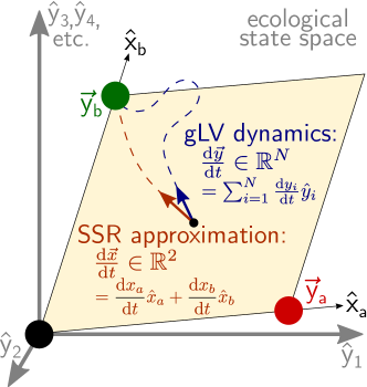
Figure 1: Schematic of Steady State Reduction (SSR). A gLV system of $N$ species (Eq. (1)) exhibits two steady states $\vec{y}_{a}$ and $\vec{y}_{b}$, characterized as diseased (red) and healthy (green). SSR identifies the two-dimensional (2D) gLV system defined on the 2D subspace spanned by the two high-dimensional steady states (Eq. (2)) that best approximates the high-dimensional system. Specifically, SSR prescribes 2D parameters (Eq. (3)) that minimize the deviation between the N-dimensional gLV dynamics $\text{d}\vec{y}/\text{d}t$ and the embedded 2D SSR-reduced dynamics $\text{d}\vec{x}/\text{d}t$.

We begin by demonstrating how to compress the high-dimensional ecological dynamics of the generalized Lotka-Volterra (gLV) equations, given in Eq. (1), into an approximate two-dimensional (2D) subspace. This process, called Steady State Reduction (SSR), is depicted schematically in Fig. 1. The idea behind SSR is to recast a pair of fixed points of a high-dimensional gLV model as idealized ecological species in a 2D gLV model, and to characterize the interactions between these two composite states by taking a weighted average over the species interactions of the high-dimensional system. Within this subspace, these reduced dynamics constitute the best possible 2D gLV approximation of the high-dimensional gLV dynamics.

The gLV equations model the populations of $N$ interacting ecological species $y_{i}$ as

$$\frac{\text{d}}{\text{d}t}y_{i}(t)=y_{i}(t)\left(\rho_{i}+\sum_{j=1}^{N}K_{ij}y_{j}(t)\right),$$ (1)

for $i\in 1,\ \ldots,\ N$. In vector form, these microbial dynamics are written $\frac{\text{d}\vec{y}}{\text{d}t}=\sum_{i=1}^{N}\frac{\text{d}y_{i}}{\text{d}t}\hat{y}_{i}$. Here, the growth rate of species $i$ is $\rho_{i}$, and the effect of species $j$ on species $i$ is given by the interaction term $K_{ij}$. In the following derivation, we assume this model observes distinct stable fixed points $\vec{y}_{a}$ and $\vec{y}_{b}$.

Define variables $x_{a}$ and $x_{b}$ in the direction of unit vectors $\hat{x}_{a}$ and $\hat{x}_{b}$ that parallel the two steady states according to $\hat{x}_{a}\equiv\vec{y}_{a}/\lVert\vec{y}_{a}\rVert_{2}$, and $\hat{x}_{b}\equiv\vec{y}_{b}/\lVert\vec{y}_{b}\rVert_{2}$, where $\lVert\cdot\rVert_{k}$ is the $k$-norm. The 2D gLV dynamics on the subspace spanned by $\hat{x}_{a}$ and $\hat{x}_{b}$ are given by

$$\begin{split}\frac{\text{d}x_{a}}{\text{d}t}&=x_{a}(\mu_{a}+M_{aa}x_{a}+M_{ab}x_{b}),\quad\text{and}\\ \frac{\text{d}x_{b}}{\text{d}t}&=x_{b}(\mu_{b}+M_{ba}x_{a}+M_{bb}x_{b}).\end{split}$$ (2)

The in-plane dynamics on this subspace in vector form are defined to be $\frac{\text{d}\vec{x}}{\text{d}t}=\frac{\text{d}x_{a}}{\text{d}t}\hat{x}_{a}+\frac{\text{d}x_{b}}{\text{d}t}\hat{x}_{b}$.

SSR links the parameters of the in-plane dynamics to the high-dimensional gLV dynamics by setting

$$\mu_{\gamma} =\frac{\vec{\rho}\cdot(\vec{y}_{\gamma}^{\ \circ 2})}{\lVert\vec{y}_{\gamma}\rVert_{2}^{2}},\quad\ \text{ for }\ \gamma\in a,\ b,\quad\text{and}$$ (3)

$$M_{\gamma\delta} =\frac{(\vec{y}_{\gamma}^{\ \circ 2})^{T}K\vec{y}_{\delta}}{\lVert\vec{y}_{\gamma}\rVert_{2}^{2}\lVert\vec{y}_{\delta}\rVert_{2}}, \text{ for }\ \gamma,\ \delta\in a,\ b.$$

Here, the Hadamard square represents the element-wise square of a vector, defined as $\vec{v}^{\ \circ 2}=[v_{1}^{2},\ v_{2}^{2},\ \ldots,\ v_{N}^{2}]^{T}$. The parameter definitions in Eq. (3) are valid when $\vec{y}_{a}$ and $\vec{y}_{b}$ are orthogonal; when they are not, the cross-interaction terms $M_{ab}$ and $M_{ba}$ become more complicated, and are given in Eqs. (28) and (29) of the Appendix.

This choice of parameters minimizes the deviation between the in-plane and high-dimensional gLV dynamics $\epsilon=\lVert\frac{\text{d}\vec{y}}{\text{d}t}-\frac{\text{d}\vec{x}}{\text{d}t}\rVert_{2}$ for any point on the subspace spanned by $\hat{x}_{a}$ and $\hat{x}_{b}$. This is proved in the Appendix by showing that, when evaluated with the SSR-prescribed parameter values of Eq. (3), $\frac{\partial\epsilon}{\partial c_{i}}=0$ for every coefficient $c_{i}\in\{\mu_{a},\ \mu_{b},\ M_{aa},\ M_{ab},\ M_{ba},\ M_{bb}\}$, and that $\frac{\partial^{2}\epsilon}{\partial c_{i}\partial c_{j}}>0$ for every pair of coefficients $c_{i}$ and $c_{j}$.

Under this construction, the high-dimensional steady states $\vec{y}_{a}$ and $\vec{y}_{b}$ have in-plane steady state counterparts at $(\lVert\vec{y}_{a}\rVert_{2},\ 0)$ and $(0,\ \lVert\vec{y}_{b}\rVert_{2})$, respectively. It is for this reason we call this method Steady State Reduction. Further, if $\vec{y}_{a}$ and $\vec{y}_{b}$ are stable and orthogonal, then the corresponding 2D steady states are stable as well, which guarantees the existence of a separatrix in the reduced 2D system. These properties are shown in the Supplementary Information , which includes many other calculations that accompany the results of this paper. We provide a Python module that implements SSR on arbitrary high-dimensional gLV systems in the Supplementary Code .

If the ecological dynamics of the system lie entirely on the plane spanned by $\hat{x}_{a}$ and $\hat{x}_{b}$, the SSR approximation is exact. In this case, the plane contains a slow manifold on which the ecological dynamics evolve. Therefore, the dynamics generated by SSR result from a linear approximation of the slow manifold.

III Steady state reduction applied to a microbiome model

Thousands of microbial species populate the gut microbiome Round and Mazmanian (2009), but for modeling purposes it is common to coarse-grain at the genus or phylum level. Recently, many experimentally derived gLV microbiome models have been constructed with tools such as MDSINE, a computational pipeline that infers gLV parameters from time-series microbial abundance data Bucci et al. (2016). SSR is applicable to any of these gLV systems, so long as it exhibits two or more stable steady states.

We consider one such experimentally derived gLV model, constructed by Stein et al. Stein et al. (2013), that studies CDI in the mouse gut microbiome. This model takes the same form as Eq. (1) and tracks the abundances of 10 different microbial genera and the pathogen C. difficile (CD), all of which can inhabit the mouse gut. The 11-dimensional (11D) parameters of this model were fit with data from an experimental mouse study Buffie et al. (2012). The parameters of this model, along with a sample microbial trajectory, are provided in the Supplementary Information Note (1).

Despite the fact that this model did not resolve individual bacterial species, it still captured the clinically- and experimentally-observed phenomenon of antibiotic-induced CDI, suggesting that the true microbiome’s dimensionality could be approximated by an 11-dimensional model. SSR further simplifies the dimensionality of the microbiome: instead of thousands of microbial species or even eleven dominant genera, with SSR steady states of the microbiome (each of which are multi-species equilibrium populations) are idealized as individual ecological populations.

This CDI model exhibits five steady states that are reachable from experimentally measured initial conditions Stein et al. (2013). In previous work, we identified which of these steady states were susceptible or resilient to invasion by C. difficile (CD) Jones and Carlson (2018). Based on this classification, we interpret a CD-susceptible steady state $\vec{y}_{a}$ of the 11D model as “diseased,” and interpret a CD-resilient steady state $\vec{y}_{b}$ as “healthy.” Explicit details about each of these states are provided in the Supplementary Information Note (1). These two states are used to demonstrate SSR.

The reduced 2D parameters are generated according to Eq. (3). We introduce new scaled variables, $z_{a}=x_{a}/\lVert\vec{y}_{a}\rVert_{2}$, and $z_{b}=x_{b}/\lVert\vec{y}_{b}\rVert_{2}$, so that the 2D system exhibits steady states at $(1,\ 0)$ and $(0,\ 1)$. In Fig. 2, trajectories of the reduced system (solid lines) that originate from four initial conditions and tend toward either the healthy (green) or diseased (red) steady states are plotted. The 2D separatrix is also plotted (light grey), which divides the basins of attraction of the two steady states, and which is derived in Eq. (4) of the Section IV.

To compare the original and reduced models, we consider 11D trajectories that originate from the 11D embedding of the four 2D initial conditions Note (1). The projections of these 11D trajectories onto the 2D subspace spanned by $\vec{y}_{a}$ and $\vec{y}_{b}$ (dashed lines) are shown alongside the corresponding 2D trajectories in Fig. 2. The in-plane 11D separatrix is also shown (dark grey), which is numerically constructed by tracking the steady state outcomes of a grid of initial conditions on the plane.

We note that $\vec{y}_{a}$ and $\vec{y}_{b}$ are nearly orthogonal. However, in the Supplementary Information we demonstrate that the high-dimensional and SSR-reduced trajectories and basins of attraction agree for four different implementations of SSR; in two of these implementations the pairs of steady states were orthogonal, and in the other two they were not Note (1). It is important to understand when SSR is a good approximation, and under what conditions it may be successfully applied— this issue will be addressed in a future publication (in progress).

In the five realizations of SSR explored in this paper and in the supplement, the basins of attraction and microbial trajectories are largely preserved through SSR. Since the 11D system has been compressed (from 132 parameters to 6), it is not surprising that the low- and projected high-dimensional trajectories do not exactly match. Even so, the basins of attraction agree almost entirely, and the dynamical trajectories share clear similarities. The deviation between the original and reduced systems is examined in more detail in the Supplementary Information Note (1). The close agreement between the original and reduced systems intimates the reductive potential of SSR.

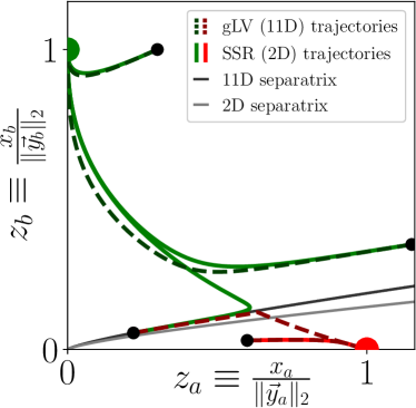
Figure 2: Fidelity of Steady State Reduction (SSR). SSR is applied to an experimentally-derived 11-dimensional (11D) gLV model of C. difficile infection (CDI) Stein et al. (2013). This model exhibits steady states $\vec{y}_{a}$ and $\vec{y}_{b}$ that are vulnerable (diseased, red) and resilient (healthy, green) to invasion by the pathogen C. difficile Note (1). We consider 11D microbial trajectories whose initial conditions lie the plane spanned by these two steady states, and plot the in-plane projection of these trajectories (dashed lines). The 2D SSR-generated dynamics (solid lines) are plotted alongside these high-dimensional trajectories. The separatrix of each system is also plotted: as a proxy for the 11D separatrix (actually a 10-dimensional surface), the in-plane separatix (dark grey) is numerically generated and plotted; the 2D separatrix is exact and given in Eq. (4) (light grey). The code used to generate this figure is available in the Supplemental Code Note (2).

IV Analysis of the 2D gLV equations

Having demonstrated a method of linking a high-dimensional gLV system to a 2D gLV system via SSR, we now take advantage of the analytic accessibility of such 2D systems. We consider biologically relevant systems that exhibit competitive dynamics by assuming $\mu_{\alpha}>0$ for $\alpha\in a,\ b$, and $M_{\alpha\beta}<0$ for $\alpha,\ \beta\in a,\ b$. These systems exhibit two stable and homogeneous fixed points at $(-\mu_{a}/M_{aa},\ 0)$ and $(0,\ -\mu_{b}/M_{bb})$. In this case, the system will also possess a hyperbolic fixed point at $(x_{a}^{*},\ x_{b}^{*})$ with $x_{a}>0$ and $x_{b}>0$, which topologically guarantees the existence of a separatrix.

In Section IV.1 this separatrix is explicitly calculated for the 2D gLV system Eq. (2). This result, in conjunction with SSR, allows for an efficient approximation of the high-dimensional separatrix. Then, Section IV.2 explores the steady state and transient dynamics of a nondimensionalized form of the 2D gLV system with clinically-inspired modifications.

IV.1 Explicit form of the separatrix

The long-term dynamics of this system are dictated by the basins of attraction of the stable steady states, and these basins are delineated by a separatrix that, for topological reasons, must be the stable manifold of the hyperbolic fixed point $(x_{a}^{*},\ x_{b}^{*})$. In Fig. 3 these basins are depicted topographically via isoclines of the split Lyapunov function $V(x_{a},x_{b})$ (lightly shaded contours), which acts as a potential energy landscape Note (1); Hou et al. (2013).

The separatrix $h(x_{a})$ may be analytically computed in a power series expansion about the hyperbolic fixed point $(x_{a}^{*},\ x_{b}^{*})$,

$$h(x_{a})=\sum_{n=0}^{\infty}\frac{c_{n}}{n!}(x_{a}-x_{a}^{*})^{n},$$ (4)

which as an invariant manifold must satisfy Wiggins (2003)

$$\frac{\text{d}h(x_{a})}{\text{d}x_{a}}=\frac{\text{d}x_{b}}{\text{d}t}\bigg{/}\frac{\text{d}x_{a}}{\text{d}t},$$ (5)

resulting in the recursive relations

$$\begin{split}c_{0}&=x_{b}^{*},\\ c_{1}&=\frac{1}{2M_{ab}x_{a}^{*}}\left[M_{bb}x_{b}^{*}-M_{aa}x_{a}^{*}\vphantom{\sqrt{1^{2}}}\right.\\ &\quad\quad\quad\left.-\sqrt{(M_{bb}x_{b}^{*}-M_{aa}x_{a}^{*})^{2}+4M_{ab}M_{ba}x_{a}^{*}x_{b}^{*}}\right],\\ c_{2}&=\frac{2c_{1}(M_{ba}+M_{bb}c_{1}-M_{aa}-M_{ab}c_{1})}{2x_{a}^{*}M_{aa}+3x_{a}^{*}M_{ab}c_{1}-M_{bb}x_{b}^{*}},\quad\text{ and}\\ c_{n}&=\frac{1}{\left(nx_{a}^{*}M_{aa}+(n+1)x_{a}^{*}M_{ab}c_{1}-M_{bb}x_{b}^{*}\right)}\\ &\quad\times\left\{nc_{n-1}(M_{ba}+M_{bb}c_{1}-(n-1)(M_{aa}+M_{ab}c_{1}))\vphantom{\sum_{i}^{1}}\right.\\ &\quad+n!\sum_{\ell=2}^{n-1}\left[\frac{c_{\ell}}{\ell!\ (n-\ell)!}\left(M_{bb}c_{n-\ell}-(n-\ell)M_{ab}c_{n-\ell}\right.\right.\\ &\quad\quad\quad\quad\quad\quad\left.\left.\left.-x_{a}^{*}M_{ab}c_{n-\ell+1}\right)\vphantom{\frac{1}{2}}\right]\vphantom{\sum_{1}^{2}}\right\},\quad\text{ for }n>2,\\ \end{split}$$ (6)

as derived in Eqs. (S27-S38) Note (1). This calculation allows the a priori classification of the fate of a given initial condition, without need for simulation. We note that this algebraic calculation of the separatrix is considerably faster than numerical methods that rely on relatively costly quadrature computations. Further, in conjunction with SSR, this analytic form offers an efficient approximation to the in-plane separatrix of high-dimensional systems.

IV.2 Dynamical landscape of the 2D gLV equations

Next, we analyze a two-state implementation of the gLV equations that parallels the clinically-inspired scenario of antibiotic-induced CDI. In this scenario, antibiotics deplete a health-prone initial condition, requiring administration of FMT in order to recover, as in Fig. 3. FMT is implemented in the 2D gLV model by adding a transplant of size $s$ composed of the healthy steady state $(0,\ 1)$ to an evolving microbial state at a specified time following administration of antibiotics.

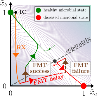
Figure 3: The success or failure of fecal microbiota transplantation (FMT) depends on the timing of its administration in a two-state gLV system (Eq. (7)). We consider a clinically-inspired scenario that parallels antibiotic-induced CDI. First, a health-prone initial condition (IC) is depleted by antibiotics (RX, orange). If FMT (brown) is administered shortly after the antibiotics, the treatment steers the composition to a healthy state (FMT success). If FMT administration is delayed, the microbial trajectory instead attains the diseased state (FMT failure). The basins of attraction of the healthy and diseased steady states are delineated by the separatrix Eq. 4, and isoclines of the potential energy landscape (light contours) are given by the split Lyapunov function Eq. (S47) Hou et al. (2013); Note (1).

We consider a nondimensionalized form of the gLV equations Eq. (2) and designate nondimensionalized variables with a tilde Note (1). Therapeutic interventions of antibiotics and FMT are included in this model in a manner consistent with previous approaches Stein et al. (2013); Jones and Carlson (2018). In all, this clinically-inspired two-state gLV model is given by

$$\begin{split}\frac{\text{d}\tilde{x}_{a}}{\text{d}t}&=\tilde{x}_{a}(1-\tilde{x}_{a}-\tilde{M}_{ab}\tilde{x}_{b})\\ &\quad+\tilde{x}_{a}\varepsilon_{a}u(t)+w_{a}\delta(t-t^{*}),\ \text{ and}\\ \frac{\text{d}\tilde{x}_{b}}{\text{d}t}&=\tilde{x}_{b}(\mu_{b}-\tilde{M}_{ba}\tilde{x}_{a}-\tilde{x}_{b})\\ &\quad+\tilde{x}_{b}\varepsilon_{b}u(t)+w_{b}\delta(t-t^{*}),\end{split}$$ (7)

which includes optional antibiotic administration $u(t)$ operating with efficacy $\vec{\varepsilon}$, and optional FMT with transplant $\vec{w}$ administered instantaneously at time $t^{*}$.

In the absence of antibiotics and FMT, the dynamical system Eq. (7) exhibits three nontrivial steady states at $(1,\ 0)$, $(0,\ \mu_{b})$, and $(\tilde{x}_{a}^{*},\ \tilde{x}_{b}^{*})\equiv(\frac{1-\tilde{M}_{ab}\tilde{\mu}_{b}}{1-\tilde{M}_{ab}\tilde{M}_{ba}},\ \frac{\tilde{\mu}_{b}-\tilde{M}_{ba}}{1-\tilde{M}_{ab}\tilde{M}_{ba}})$. To simplify the presentation of our results in the main text we assume $\mu_{b}=1$, though this assumption is relaxed in the Supplementary Information Note (1).

As before, suppose the variable $\tilde{x}_{a}$ corresponds to a diseased state, and $\tilde{x}_{b}$ corresponds to a healthy state. Also assume the transplant $\vec{w}$ consists of exclusively healthy microbes so that $w_{a}=0$. Figs. 3, 4, and 5 are generated with parameter values $\tilde{M}_{ab}=1.167$ and $\tilde{M}_{ba}=1.093$, which give typical results.

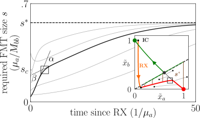
Figure 4: The FMT transplant size needed to revert an antibiotic-depleted state back to health grows as FMT administration is delayed. The minimum FMT transplant size required to cure five distinct disease-prone microbial trajectories, each evolving according to Eq. (7), are calculated and plotted. As trajectories attain the diseased steady state, the required transplant size approaches $s^{*}$. The required transplant size changes at two different rates, $\alpha$ and $\beta$, with the crossover point between these two rates at size $s_{c}$ indicated by a hollow square. The transplant size dynamics $\text{d}s/\text{d}t$ as well as the rates $\alpha$ and $\beta$ are derived in Eq. (9) and the surrounding text.

Altering the fate of an initial condition requires crossing the separatrix by some external means, which is achieved through FMT. Fig. 3 shows two microbial time courses in which long-term outcomes are determined by the timing of FMT administration. At each point along a microbial trajectory in the diseased basin of attraction, the minimum FMT size $s$ required to transfer the microbial state into the healthy basin of attraction is calculated. We use this metric to quantify our notions of “FMT efficacy.”

In clinical practice FMT administration varies in transplant size, transplant composition, and how many transplants are performed. Further, it is unclear how these factors influence the success of FMT Hota and Poutanen (2018). For the purposes of this paper, we consider a hypothetical FMT treatment of size $s_{t}$ (i.e. a horizontal cut across Fig. 4) and describe how its success depends on the timing of its administration.

Fig. 4 presents the minimum FMT size $s$ as a function of time (main panel) for several trajectories that originate in the diseased basin of attraction (inset), including the main trajectory of Fig. 3. This minimum required FMT size increases with time— often dramatically— and there are two discernible rates of increase, denoted $\alpha$ and $\beta$ in Fig. 4. These two rates are related to the fast and slow manifolds of the ecological system, which in turn govern the minimum required transplant size dynamics over time.

To reflect the importance of the separatrix in dictating the microbial dynamics, we change coordinates to the eigenvectors $(u,\ v)$ of the hyperbolic steady state, shown in Fig. 5 (inset). In these coordinates the $v$-axis corresponds to the separatrix, and $u$ is proportional to the minimum FMT size required for a successful transplant $s$, such that $s=u/(\hat{u}\cdot\hat{x}_{b})$, where $(\hat{u},\ \hat{v})$ and $(\hat{x}_{a},\ \hat{x}_{b})$ are the unit vectors associated with their associated coordinates.

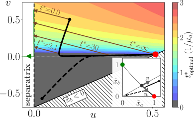
Figure 5: The role of timing in FMT administration. For antibiotic-depleted disease-prone initial conditions in which antibiotics have been cleared ($u(t)=0$), FMT is most effective when administered immediately ($t^{*}_{\text{opt}}=0$, grey) or nearly immediately ($t^{*}_{\text{opt}}>0$, colored) following antibiotic administration. The optimal transplant time $t^{*}_{\text{opt}}$ is computed for any initial condition ($u_{0},\ v_{0}$) (colorbar) according to Eq. (S88) of Note (1), which can reduce to Eq. (10). Two representative microbial trajectories are plotted in $(u,\ v)$ (main panel) and $(x_{a},\ x_{b})$ (inset) coordinates. For $v_{0}>0$ four possible FMT transplants are shown, including the optimal one that occurs at $t^{*}_{\text{opt}}=2.1$. For $v_{0}<0$ it is always best to administer FMT immediately following antibiotic administration.

In this new $(u,v)$ basis, the 2D gLV equations become

$$\begin{split}\frac{\text{d}u}{\text{d}t}&=A_{10}u-A_{11}uv-A_{20}u^{2},\quad\text{and}\\ \frac{\text{d}v}{\text{d}t}&=-B_{01}v-B_{02}v^{2}+B_{20}u^{2},\end{split}$$ (8)

where each coefficient is a positive algebraic function of the original gLV parameters given analytically in Eqs. (S60-S74) Note (1). When $\mu_{b}\neq 1$, these equations contain additional quadratic terms described in Note (1) that account for the nonlinearity of the separatrix. In the small $u$ and small $v$ limit this model reduces to the linearization about the hyperbolic fixed point. Near this fixed point there is a separation of time scales between $u$ and $v$ ($B_{01}/A_{10}>1$ always, with median of 5.9 and IQR of [2.7, 9.1] over random parameter draws Note (1)), indicating that there are inherent fast and slow manifolds in this system.

This coordinate change also reveals the role of timing in FMT administration, since the minimum required transplant size $s$ is precisely governed by Eq. (8), by proxy of $u$. To demonstrate this analytically, we consider an initial condition condition $(u_{0},\ v_{0})$ that is located near the fast manifold in a system with clear separation of time scales, so that (i) $B_{20}u_{0}^{2}$ is negligible, (ii) $A_{10}<<B_{01}$, and (iii) $B_{02}v_{0}^{2}<<B_{01}v_{0}$ (though this assumption is relaxed in Eq. (S87) Note (1)). In this case, the dynamics in the fast $\hat{v}$ direction are approximately $v(t)\approx v_{0}\text{e}^{-B_{01}t}$, and the required transplant size dynamics reduce to

$$\frac{\text{d}s}{\text{d}t}=s\left(A_{10}-A_{20}(\hat{u}\cdot\hat{x}_{b})s-A_{11}v_{0}\text{e}^{-B_{01}t}\right).$$ (9)

Thus, the required transplant size rates $\alpha$ and $\beta$ in Fig. 4 are approximately $\alpha=\frac{\text{d}s(0)}{\text{d}t}\big{|}_{s=s_{c}}$, and $\beta=\frac{\text{d}s(\infty)}{\text{d}t}\big{|}_{s=s_{c}}$, where $s_{c}$ is the transplant size required at the crossover point between these rates (e.g. as shown in Fig. 4).

For an initial condition with $v_{0}<0$, which occurs in Fig. 3 when a nearly healthy state is depleted by antibiotics, $\alpha>\beta$. In this case the required transplant size monotonically increases until it attains $s^{*}$ at the infected steady state, so it is best to administer FMT as soon as possible. Alternatively, when $v_{0}>0$, $\alpha<\beta$. When $A_{11}v_{0}$ is sufficiently large $\alpha$ becomes negative, which indicates there is a nonzero transplant time at which the required transplant size is minimized (corresponding to $\frac{\text{d}s}{\text{d}t}=0$). The concave-up trajectories in Fig. 4 exhibit this optimal transplant time. For $v_{0}>0$ and under the same conditions for which Eq. (9) was derived, this optimal transplant time $t^{*}$ is

$$t^{*}_{\text{opt}}=\frac{1}{B_{01}}\ln\left(\frac{A_{11}v_{0}}{A_{10}-A_{20}u_{0}}\right).$$ (10)

This nonzero transplant time reflects ecological pressures that temporarily drive the system closer to the separatrix, overpowering the slow unstable manifold. Two trajectories that numerically recapitulate these two cases are shown in Fig. 5.

V SSR applied to fecal microbiota transplantation

Figure 6: Transient dynamics are preserved under SSR. (inset) Microbial trajectories of the CDI model (in-plane projection, dashed) and the associated SSR-reduced model (solid) as in Fig. 2 are shown. (main panel) At each time along these trajectories, the minimum FMT size required to make the state health-prone is plotted, for a transplant made up of $\vec{y}_{b}$ (11D, dashed) or $(0,\ 1)$ (2D, solid). Phase space is linked to the FMT size dynamics by indicating the time at which $z_{b}$ begins to decrease with a solid square (2D) or diamond (11D) in both the inset and main figure. Since the required FMT size $s$ is the distance between a state and the separatrix, the similarity between the two time courses of $s$ indicates that SSR preserves transient dynamics.

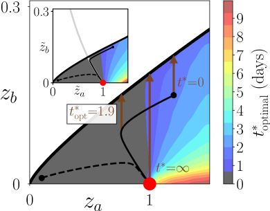
Figure 7: Optimal transplant times are preserved under SSR. Optimal transplant times $t^{*}_{\text{opt}}$ of the 11D Stein model (main panel) largely match the predictions of its associated SSR-reduced model (inset). In the high-dimensional model, $t^{*}_{\text{opt}}$ is computed numerically (as in Fig. 6) for a grid of points on the plane spanned by $\vec{y}_{a}$ and $\vec{y}_{b}$ for disease-prone initial conditions (located underneath the separatrix, which is shown as a thick black line). The spatial and temporal resolutions of this simulation are $\delta z_{a}=0.025$, $\delta z_{b}=0.01$, and $\delta t_{\text{opt}}=0.15$, and the resulting data points were smoothed with a Gaussian filter. (inset) We display the optimal transplant times of the corresponding SSR-reduced model, as in Fig. 5. The SSR-reduced parameters were nondimensionalized so that $t^{*}_{\text{opt}}$ could be generated with Eq. (S88), and the resulting optimal transplant time predictions were redimensionalized and plotted. The inset and the main panel share the same colorbar.

In Section IV, FMT restored a CDI-prone microbial state in a 2D gLV model. In previous work Jones and Carlson (2018), we implemented FMT in the previously mentioned 11D CDI model Stein et al. (2013) and observed similar success. Here, the behavior of FMT in the CDI model and in its SSR counterpart are shown to match closely, which indicates that SSR preserves transient microbial dynamics.

Fig. 6 (inset) contains the in-plane projections of the 11D (dashed) and corresponding SSR-reduced 2D (solid) microbial trajectories with initial conditions that lie on the plane spanned by $(\hat{y}_{a},\ \hat{y}_{b})$ (11D) and $(\hat{z}_{a},\ \hat{z}_{b})$ (2D), as in Fig. 2. Fig. 6 (main panel) plots the required transplant size $s$ at each state along the two trajectories: the 11D (dashed) transplant is composed of $\hat{y}_{a}$, and $s$ is calculated numerically with a bisection method; the 2D (solid) transplant is composed of $\hat{z}_{b}=(0,\ 1)$, and $s$ is computed analytically with Eq. (4).

In both systems, the microbial trajectories follow a fast stable manifold before switching to a slow manifold of some hyperbolic fixed point. As in the 2D case, the flow along these fast and slow manifolds underpins how the required transplant size $s$ changes over time. In Fig. 6, the transition between the fast and slow manifolds occurs at 8.37 days in 11D (solid diamond, main panel and inset) and at 8.31 days in 2D (solid square).

As in the 2D case, the transition between these manifolds may result in a nonzero optimal transplant time $t^{*}_{\text{opt}}$. The main panel of Fig. 7 displays these optimal transplant times over a range of initial conditions, in which $t^{*}_{\text{opt}}$ is generated with the same numerical bisection method as previously mentioned. Many of the high-dimensional initial conditions exhibit a non-zero optimal transplant time, mirroring the results of Fig. 5. Further, the high-dimensional optimal transplant times closely match those predicted by SSR, which are displayed in the inset of Fig. 7, and which were analytically calculated with Eq. (S88).

Since the SSR-reduced system largely preserves the high-dimensional transplant time dynamics, and since in the 2D nondimensionalized system $t^{*}_{\text{opt}}$ can be examined analytically, the high-dimensional optimal transplant times may be approximated in terms of the high-dimensional interaction parameters. First, for systems well-approxiated by SSR, a nonzero optimal transplant time can only exist when $v_{0}>0$— this tends to occur when the size of the initial condition is larger than that of the steady state $\vec{y}_{b}$, and when its composition is similar to that of $\vec{y}_{b}$. For this class of initial conditions, $t_{\text{opt}}$ will be smaller when the eigenvalues of the semistable fixed point ($A_{10}$ and $B_{01}$) are larger, or in terms of the SSR-reduced parameters, when $M_{ab}/M_{bb}$ and $M_{ba}/M_{aa}$ are larger.

The similarities between the transient dynamics of the high-dimensional and 2D systems, as well as the correspondence in optimal transplant timings, suggest that the theoretical analyses of Section IV may inform more complex and highly-resolved systems.

VI Discussion

VI.1 Compression of complex ecological systems

SSR differs from other model reduction techniques Gu (2011); Goeke et al. (2017) since it preserves core observable ecological features of the original model, namely steady states and their stabilities. The behavior of the model on the transition between two of these steady states is approximated by SSR. Though the implementations of SSR demonstrated in this paper were accurate, in general the accuracy of SSR is not obvious a priori; therefore, in future work it is important to carefully examine the circumstances under which SSR is effective. When SSR is accurate, properties of the steady states the original model may also be extracted from this approximation— for example, the size of the basins of attraction in the approximate system can inform the robustness of a given state in the original system, and the separatrix of the reduced model can approximate the slow manifold on which dynamics evolve in the original model. The speed-up gained by leveraging the analytic tractability of these approximate systems highlights the utility of SSR.

Beyond applications to existing gLV models, SSR-based methods could create two-state gLV systems from raw microbial data by choosing basis vectors during the fitting process that correspond to experimentally observed steady states Costea et al. (2018). The resulting models would describe interactions between steady states rather than between individual species, and would consist of fewer variables and parameters that have improved explanatory power. This perspective— which effectively changes the basis vectors of a gLV model from species to steady states— may inform the transitions between steady states in ecological models.

VI.2 Simplification of gLV-based FMT frameworks

Bacteriotherapy is a promising frontier of medicine that relies on the notion that the microbiome’s composition can both influence and be influenced by disease. Then, the deliberate alteration of a dysbiotic microbiome, by FMT for example, might be a viable treatment option for a range of diseases Young (2017); Belizário and Napolitano (2015). Since FMT does not contribute to antimicrobial resistance, it is an emerging alternative to antibiotics Borody and Khoruts (2011); Heath et al. (2018). Clinical studies continue to regularly identify new diseases that are treated by FMT Hudson et al. (2017); Bilinski et al. (2017); Taur et al. (2018).

In this paper we examined a bistable two-state gLV model from a clinical perspective, in which interventions such as FMT or antibiotics altered the outcome of a microbial trajectory. The tractability of this two-state system allowed for an explicit understanding of how the efficacy of FMT is influenced by the timing of its administration following antibiotic treatment. In this model, delaying the administration of FMT in disease-prone microbiomes could lead to its failure. Modifying the time course of a treatment has innovated treatment strategies in cancer immunotherapy Messenheimer et al. (2017) and HIV vaccination Wang (2017), and the results of this two-state ecological model suggest that treatment timing may be relevant for bacteriotherapy as well.

Indeed, some circumstantial evidence exists that supports the predictions of the two-state model, in which FMT efficacy is improved when administered shortly after antibiotics. Kang et al. Kang et al. (2017) used a promising variant of FMT to induce seemingly long-term changes in the microbiome and symptoms of children with autism spectrum disorders. This FMT variant “Microbiota Transfer Therapy” first prescribed the antibiotic vancomycin for two weeks, then bowel cleaning, then a large FMT dose of Standardized Human Gut Microbiota, and finally two months of daily maitenance FMT doses. In their study, they intended for the efficacy of FMT to be improved by first clearing out the microbiome with antibiotics, which is consistent with the results of the 2D gLV system. However, future experiments are needed to quantitatively test the extent to which antibiotic-depleted states are receptive to FMT-like therapies.

VII Conclusion

Broadly, SSR realizes a progression towards the simplification of dynamical systems: while linearization approximates a dynamical system about a single steady state, SSR approximates a dynamical system about two steady states. We have shown that SSR produces the best possible in-plane 2D gLV approximation to high-dimensional gLV dynamics. Further, we have demonstrated the extent to which the 2D model captures the basins of attraction and transient dynamics of an experimentally derived model. In addition to the computational efficiency of this technique, which employs analytic results rather than expensive simulations, SSR builds an intuition for the high-dimensional system out of connected 2D cross-sections.

By approximating this complex and classic ecological model with analytically tractable ecological subspaces, SSR anchors a high-dimensional system to well-characterized 2D systems. Consequently, this technique offers to unravel the complicated landscapes that accompany complex systems and their behaviors.

*

Appendix A Derivation of Steady State Reduction

Consider an N-dimensional gLV system given by Eq. (1) that exhibits steady states $\vec{y}_{a}$ and $\vec{y}_{b}$, with dynamics given by $\frac{\text{d}\vec{y}}{\text{d}t}=\sum_{i=1}^{N}\frac{\text{d}y_{i}}{\text{d}t}\hat{y}_{i}$. As in the main text, define variables $x_{a}$ and $x_{b}$ in the direction of the unit vectors $\hat{x}_{a}\equiv\vec{y}_{a}/\lVert\vec{y}_{a}\rVert_{2}$, and $\hat{x}_{b}\equiv\vec{y}_{b}/\lVert\vec{y}_{b}\rVert_{2}$, where $\lVert\cdot\rVert_{k}$ is the $k$-norm. Further consider the in-plane 2D gLV dynamics that exist on the plane spanned by $\hat{x}_{a}$ and $\hat{x}_{b}$. Here, we prove that the parameters prescribed by Steady State Reduction, given in Eq. (3), minimize the 2-norm of the deviation $\vec{\epsilon}$ between the high-dimensional and in-plane dynamics at every point on the plane.

Consider coefficients $\textbf{c}=\{c_{1},\ \ldots,\ c_{6}\}$ that parameterize the 2D gLV equations,

$$\begin{split}\frac{\text{d}x_{a}}{\text{d}t}&=x_{a}\left(c_{1}+c_{2}x_{a}+c_{3}x_{b}\right),\quad\text{and}\\ \frac{\text{d}x_{b}}{\text{d}t}&=x_{b}\left(c_{4}+c_{5}x_{a}+c_{6}x_{b}\right),\end{split}$$ (11)

so that the in-plane dynamics are $\frac{\text{d}\vec{x}}{\text{d}t}=\frac{\text{d}x_{a}}{\text{d}t}\hat{x}_{a}+\frac{\text{d}x_{b}}{\text{d}t}\hat{x}_{b}$. Any point on this plane can be written $\vec{y}=\vec{y}_{a}x_{a}+\vec{y}_{b}x_{b}$.

The deviation between the high-dimensional and in-plane dynamics $\vec{\epsilon}$ is

$$\vec{\epsilon}(x_{a},\ x_{b})=\frac{\text{d}\vec{x}}{\text{d}t}-\frac{\text{d}\vec{y}}{\text{d}t},$$ (12)

which is defined at every point on the plane $(x_{a},\ x_{b})$. We will show that the parameters precribed by SSR minimize the 2-norm of this deviation $\lVert\vec{\epsilon}\rVert_{2}$ at point on the plane.

The deviation $\vec{\epsilon}$ can be decomposed into the N-dimensional unit vectors $\hat{y}_{i}$, so that $\vec{\epsilon}=\sum_{i}\hat{y}_{i}\epsilon_{i}$, where the components $\epsilon_{i}$ are given by

$$\begin{split}\epsilon_{i}&=y_{ai}x_{a}\left((c_{1}-\rho_{i})+\left(c_{2}-\sum_{j=1}^{N}K_{ij}y_{aj}\right)x_{a}+\left(c_{3}-\sum_{j=1}^{N}K_{ij}y_{bj}\right)x_{b}\right)\\ &\quad\quad\quad\ +y_{bi}x_{b}\left((c_{4}-\rho_{i})+\left(c_{5}-\sum_{j=1}^{N}K_{ij}y_{aj}\right)x_{a}+\left(c_{6}-\sum_{j=1}^{N}K_{ij}y_{bj}\right)x_{b}\right)\\ &\equiv\epsilon_{10,i}x_{a}+\epsilon_{20,i}x_{a}^{2}+\epsilon_{11,i}x_{a}x_{b}+\epsilon_{01,i}x_{b}+\epsilon_{02,i}x_{b}^{2},\end{split}$$ (13)

where components $\epsilon_{jk,i}$ are defined to correspond to contributions by $x_{a}^{j}x_{b}^{k}$ terms. Here, $y_{ai}$ corresponds to the $i$th component of the unit vector $\hat{x}_{a}\equiv\vec{y}_{a}/\lVert\vec{y}_{a}\rVert_{2}$. In the same way, the deviation vector may be decomposed according to

$$\vec{\epsilon}=\vec{\epsilon}_{10}x_{a}+\vec{\epsilon}_{20}x_{a}^{2}+\vec{\epsilon}_{11}x_{a}x_{b}+\vec{\epsilon}_{01}x_{b}+\vec{\epsilon}_{02}x_{b}^{2}.$$ (14)

Minimizing this deviation at each point $(x_{a},\ x_{b})$ is equivalent to minimizing each orthogonal contribution $\vec{\epsilon}_{jk}$. Each contribution is a function of one or two parameters ($\vec{\epsilon}_{10}(c_{1})$, $\vec{\epsilon}_{20}(c_{2})$, $\vec{\epsilon}_{01}(c_{4})$, $\vec{\epsilon}_{02}(c_{6})$, and $\vec{\epsilon}_{11}(c_{3},\ c_{5})$), which simplifies the minimization process.

We now find the set of optimal coefficients $\textbf{c}^{*}=\{c_{1}^{*},\ \ldots,\ c_{6}^{*}\}$ that minimize the 2-norm of each contribution $\lVert\vec{\epsilon}_{jk}\rVert_{2}$. For convenience, we equivalently minimize the square of this 2-norm. The Hadamard square represents the element-wise square of a vector, defined as $\vec{v}^{\ \circ 2}=[v_{1}^{2},\ v_{2}^{2},\ \ldots,\ v_{N}^{2}]^{T}$.

The coefficient $\lVert\vec{\epsilon}_{10}\rVert_{2}^{2}$ is given by

$$\lVert\vec{\epsilon}_{10}\rVert_{2}^{2}=\sum_{i=1}^{N}y_{ai}^{2}(c_{1}-\rho_{i})^{2}.$$ (15)

When minimized with respect to $c_{1}$, this quantity obeys

$$\frac{\text{d}\lVert\vec{\epsilon}_{10}\rVert_{2}^{2}}{\text{d}c_{1}}=\sum_{i=1}^{N}2y_{ai}^{2}(c_{1}-\rho_{i})=0,$$ (16)

which is satified for

$$c_{1}^{*}=\frac{\sum_{i=1}^{N}y_{ai}^{2}\rho_{i}}{\sum_{i=1}^{N}y_{ai}^{2}}=\frac{\vec{y}_{a}^{\ \circ 2}\cdot\vec{\rho}}{\lVert\vec{y}_{a}\rVert_{2}^{2}}.$$ (17)

In a similar way, $\lVert\vec{\epsilon}_{20}\rVert_{2}^{2}$, $\lVert\vec{\epsilon}_{01}\rVert_{2}^{2}$, and $\lVert\vec{\epsilon}_{02}\rVert_{2}^{2}$ are minimized when

$$\begin{split}c_{2}^{*}&=\frac{\sum_{i=1}^{N}\left(y_{ai}^{2}\sum_{j=1}^{N}K_{ij}y_{aj}\right)}{\sum_{i=1}^{N}y_{ai}^{2}}=\frac{(\vec{y}_{a}^{\ \circ 2})^{T}K\vec{y}_{a}}{\lVert\vec{y}_{a}\rVert_{2}^{3}},\end{split}$$ (18)

$$\begin{split}c_{4}^{*}=\frac{\sum_{i=1}^{N}y_{bi}^{2}\rho_{i}}{\sum_{i=1}^{N}y_{bi}^{2}}=\frac{\vec{y}_{b}^{\ \circ 2}\cdot\vec{\rho}}{\lVert\vec{y}_{b}\rVert_{2}^{2}},\end{split}$$ (19)

and

$$\begin{split}c_{6}^{*}&=\frac{\sum_{i=1}^{N}\left(y_{bi}^{2}\sum_{j=1}^{N}K_{ij}y_{bj}\right)}{\sum_{i=1}^{N}y_{bi}^{2}}=\frac{(\vec{y}_{b}^{\ \circ 2})^{T}K\vec{y}_{b}}{\lVert\vec{y}_{b}\rVert_{2}^{3}}.\end{split}$$ (20)

Lastly, the squared norm of the cross-term $\lVert\vec{\epsilon}_{11}\rVert_{2}$ is given by

$$\begin{split}\lVert\vec{\epsilon}_{11}\rVert_{2}^{2}&=\sum_{i=1}^{N}\left[y_{ai}\left(c_{3}-\sum_{j=1}^{N}K_{ij}y_{bj}\right)\right.\\ &\quad\quad\ \quad\left.+y_{bi}\left(c_{5}-\sum_{j=1}^{N}K_{ij}y_{aj}\right)\right]^{2}.\end{split}$$ (21)

Minimizing with respect to $c_{3}$ and $c_{5}$ results in

$$\begin{split}\frac{\text{d}\lVert\vec{\epsilon}_{11}\rVert_{2}^{2}}{\text{d}c_{3}}&=\sum_{i=1}^{N}2\left[y_{ai}^{2}\left(c_{3}-\sum_{j=1}^{N}K_{ij}y_{bj}\right)\right.\\ &\quad\quad\ \ \quad\left.+y_{ai}y_{bi}\left(c_{5}-\sum_{j=1}^{N}K_{ij}y_{aj}\right)\right]\\ &=0,\end{split}$$ (22)

and

$$\begin{split}\frac{\text{d}\lVert\vec{\epsilon}_{11}\rVert_{2}^{2}}{\text{d}c_{5}}&=\sum_{i=1}^{N}2\left[y_{ai}y_{bi}\left(c_{3}-\sum_{j=1}^{N}K_{ij}y_{bj}\right)\right.\\ &\quad\quad\ \ \quad\left.+y_{bi}^{2}\left(c_{5}-\sum_{j=1}^{N}K_{ij}y_{aj}\right)\right]\\ &=0.\end{split}$$ (23)

After rearranging terms, these conditions read

$$\begin{split}c_{3}\sum_{i=1}^{N}y_{ai}^{2}+c_{5}\sum_{i=1}^{N}y_{ai}y_{bi}&=\sum_{i=1}^{N}\sum_{j=1}^{N}y_{ai}K_{ij}(y_{ai}y_{bj}+y_{bi}y_{aj}),\end{split}$$ (24)

and

$$\begin{split}c_{3}\sum_{i=1}^{N}y_{ai}y_{bi}+c_{5}\sum_{i=1}^{N}y_{bi}^{2}&=\sum_{i=1}^{N}\sum_{j=1}^{N}y_{bi}K_{ij}(y_{ai}y_{bj}+y_{bi}y_{aj}),\\ \end{split}$$ (25)

which are satisfied when

$$\begin{split}c_{3}^{*}&=\frac{\sum_{i,j=1}^{N}K_{ij}(y_{ai}y_{bj}+y_{bi}y_{aj})\left(\sum_{k=1}^{N}y_{ai}y_{bk}^{2}-y_{bi}y_{ak}y_{bk}\right)}{\left(\sum_{i=1}^{N}y_{ai}^{2}\right)\left(\sum_{i=1}^{N}y_{bi}^{2}\right)-\left(\sum_{i=1}^{N}y_{ai}y_{bi}\right)^{2}},\\ \end{split}$$ (26)

and

$$\begin{split}c_{5}^{*}&=\frac{\sum_{i,j=1}^{N}K_{ij}(y_{ai}y_{bj}+y_{bi}y_{aj})\left(\sum_{k=1}^{N}y_{bi}y_{ak}^{2}-y_{ai}y_{ak}y_{bk}\right)}{\left(\sum_{i=1}^{N}y_{ai}^{2}\right)\left(\sum_{i=1}^{N}y_{bi}^{2}\right)-\left(\sum_{i=1}^{N}y_{ai}y_{bi}\right)^{2}}.\\ \end{split}$$ (27)

However, when $\vec{y}_{a}$ and $\vec{y}_{b}$ are orthogonal, the cross-term deviation $\lVert\vec{\epsilon}_{11}\rVert_{2}^{2}$ is simplified, and the optimal coefficients $c_{3}^{*}$ and $c_{5}^{*}$ become

$$\begin{split}c_{3}^{*}&=\frac{\sum_{i=1}^{N}\left(y_{ai}^{2}\sum_{j=1}^{N}K_{ij}y_{bj}\right)}{\sum_{i=1}^{N}y_{ai}^{2}}=\frac{(\vec{y}_{a}^{\ \circ 2})^{T}K\vec{y}_{b}}{\lVert\vec{y}_{a}\rVert_{2}^{2}\lVert\vec{y}_{b}\rVert_{2}},\end{split}$$ (28)

and

$$\begin{split}c_{5}^{*}&=\frac{\sum_{i=1}^{N}\left(y_{bi}^{2}\sum_{j=1}^{N}K_{ij}y_{aj}\right)}{\sum_{i=1}^{N}y_{bi}^{2}}=\frac{(\vec{y}_{b}^{\ \circ 2})^{T}K\vec{y}_{a}}{\lVert\vec{y}_{b}\rVert_{2}^{2}\lVert\vec{y}_{a}\rVert_{2}}.\end{split}$$ (29)

Since the squared norms of the deviations $\lVert\epsilon_{jk}\rVert_{2}$ are convex, the coefficient set c^∗ is a global minimum for $\lVert\vec{\epsilon}\rVert_{2}$. Therefore, we have identified the parameters that minimize the deviation between the in-plane and high-dimensional gLV dynamics for any point on the plane spanned by $\vec{y}_{a}$ and $\vec{y}_{b}$.

References

- Briggs et al. (2010) C. J. Briggs, R. A. Knapp, and V. T. Vredenburg, Proceedings of the National Academy of Sciences (2010).
- Bucci and Xavier (2014) V. Bucci and J. B. Xavier, Journal of Molecular Biology 426, 3907 (2014).
- Round and Mazmanian (2009) J. L. Round and S. K. Mazmanian, Nat Rev Immunol 9, 313 (2009).
- Lloyd-Price et al. (2016) J. Lloyd-Price, G. Abu-Ali, and C. Huttenhower, Genome Medicine 8, 51 (2016).
- Widder et al. (2016) S. Widder, R. J. Allen, T. Pfeiffer, T. P. Curtis, C. Wiuf, W. T. Sloan, O. X. Cordero, S. P. Brown, B. Momeni, W. Shou, H. Kettle, H. J. Flint, A. F. Haas, B. Laroche, J.-U. Kreft, P. B. Rainey, S. Freilich, S. Schuster, K. Milferstedt, J. R. van der Meer, T. Grokopf, J. Huisman, A. Free, C. Picioreanu, C. Quince, I. Klapper, S. Labarthe, B. F. Smets, H. Wang, I. N. I. Fellows, and O. S. Soyer, The Isme Journal 10, 2557 (2016).
- Papin et al. (2004) J. A. Papin, J. L. Reed, and B. O. Palsson, Trends in Biochemical Sciences 29, 641 (2004).
- Stein et al. (2013) R. R. Stein, V. Bucci, N. C. Toussaint, C. G. Buffie, G. Rätsch, E. G. Pamer, C. Sander, and J. B. Xavier, PLoS Comput Biol 9, 1 (2013).
- Buffie et al. (2012) C. G. Buffie, I. Jarchum, M. Equinda, L. Lipuma, A. Gobourne, A. Viale, C. Ubeda, J. Xavier, and E. G. Pamer, Infect Immun 80, 62 (2012).
- Jones and Carlson (2018) E. W. Jones and J. M. Carlson, PLOS Computational Biology 14, 1 (2018).
- Merenstein et al. (2014) D. Merenstein, N. El-Nachef, and S. V. Lynch, Journal of Pediatric Gastroenterology and Nutrition 59 (2014).
- Note (1) Supplementary Information available at ****.
- Note (2) Supplementary Code used to implement SSR and generate Fig. 2 available at github.com/erijones/ssr_module.
- Bucci et al. (2016) V. Bucci, B. Tzen, N. Li, M. Simmons, T. Tanoue, E. Bogart, L. Deng, V. Yeliseyev, M. L. Delaney, Q. Liu, B. Olle, R. R. Stein, K. Honda, L. Bry, and G. K. Gerber, Genome Biology 17, 121 (2016).
- Hou et al. (2013) Z. Hou, B. Lisena, M. Pireddu, F. Zanolin, S. Ahmad, and I. Stamova, Lotka-Volterra and Related Systems: Recent Developments in Population Dynamics, De Gruyter Series in Mathematics and Life Sciences (De Gruyter, 2013).
- Wiggins (2003) S. Wiggins, Introduction to applied nonlinear dynamical systems and chaos, Vol. 2 (Springer Science & Business Media, 2003).
- Hota and Poutanen (2018) S. S. Hota and S. M. Poutanen, Open Forum Infect Dis 5 (2018).
- Gu (2011) C. Gu, Model order reduction of nonlinear dynamical systems, Ph.D. thesis, UC Berkeley (2011).
- Goeke et al. (2017) A. Goeke, S. Walcher, and E. Zerz, Physica D: Nonlinear Phenomena 345, 11 (2017).
- Costea et al. (2018) P. I. Costea, F. Hildebrand, M. Arumugam, F. Bäckhed, M. J. Blaser, F. D. Bushman, W. M. de Vos, S. Ehrlich, C. M. Fraser, M. Hattori, C. Huttenhower, I. B. Jeffery, D. Knights, J. D. Lewis, R. E. Ley, H. Ochman, P. W. O’Toole, C. Quince, D. A. Relman, F. Shanahan, S. Sunagawa, J. Wang, G. M. Weinstock, G. D. Wu, G. Zeller, L. Zhao, J. Raes, R. Knight, and P. Bork, Nature Microbiology 3, 8 (2018).
- Young (2017) V. B. Young, BMJ 356 (2017).
- Belizário and Napolitano (2015) J. E. Belizário and M. Napolitano, Frontiers in Microbiology 6, 1050 (2015).
- Borody and Khoruts (2011) T. J. Borody and A. Khoruts, Nature Reviews Gastroenterology & Hepatology 9, 88 EP (2011).
- Heath et al. (2018) R. D. Heath, C. Cockerell, R. Mankoo, J. A. Ibdah, and V. Tahan, North Clin Istanb 5, 79 (2018).
- Hudson et al. (2017) L. E. Hudson, S. E. Anderson, A. H. Corbett, and T. J. Lamb, Clinical Microbiology Reviews 30, 191 (2017).
- Bilinski et al. (2017) J. Bilinski, P. Grzesiowski, N. Sorensen, K. Madry, J. Muszynski, K. Robak, M. Wroblewska, T. Dzieciatkowski, G. Dulny, J. Dwilewicz-Trojaczek, W. Wiktor-Jedrzejczak, and G. W. Basak, Clinical Infectious Diseases 65, 364 (2017).
- Taur et al. (2018) Y. Taur, K. Coyte, J. Schluter, E. Robilotti, C. Figueroa, M. Gjonbalaj, E. R. Littmann, L. Ling, L. Miller, Y. Gyaltshen, E. Fontana, S. Morjaria, B. Gyurkocza, M.-A. Perales, H. Castro-Malaspina, R. Tamari, D. Ponce, G. Koehne, J. Barker, A. Jakubowski, E. Papadopoulos, P. Dahi, C. Sauter, B. Shaffer, J. W. Young, J. Peled, R. C. Meagher, R. R. Jenq, M. R. M. van den Brink, S. A. Giralt, E. G. Pamer, and J. B. Xavier, Science Translational Medicine 10 (2018).
- Messenheimer et al. (2017) D. J. Messenheimer, S. M. Jensen, M. E. Afentoulis, K. W. Wegmann, Z. Feng, D. J. Friedman, M. J. Gough, W. J. Urba, and B. A. Fox, Clinical Cancer Research 23, 6165 (2017).
- Wang (2017) S. Wang, PLOS Computational Biology 13, 1 (2017).
- Kang et al. (2017) D.-W. Kang, J. B. Adams, A. C. Gregory, T. Borody, L. Chittick, A. Fasano, A. Khoruts, E. Geis, J. Maldonado, S. McDonough-Means, E. L. Pollard, S. Roux, M. J. Sadowsky, K. S. Lipson, M. B. Sullivan, J. G. Caporaso, and R. Krajmalnik-Brown, Microbiome 5 (2017).